Multilevel Polar Coded Space-Shift Keying

Abstract

Multilevel coding (MLC) is a coded modulation technique which can achieve excellent performance over a range of communication channels. Polar codes have been shown to be quite compatible with communication systems using MLC, as the rate allocation of the component polar codes follows the natural polarization inherent in polar codes. MLC based techniques have not yet been studied in systems that use spatial modulation (SM). SM makes the polar code design difficult as the spatial bits actually select a channel index for transmission. To solve this problem, we propose a Monte Carlo based evaluation of the ergodic capacities for the individual bit levels under the capacity rule for a space-shift keying (SSK) system, where we also make use of a single antenna activation to approximate the transmission channel for the design of the multilevel polar code. Our simulation results show that the multilevel polar coded $16\times 1$ SSK system outperforms the corresponding system that uses bit-interleaved polar coded modulation by $2.9$ dB at a bit-error rate (BER) of $10^{-4}$.

I Introduction

Multilevel coded (MLC) modulation was first introduced independently by Imai and Hirakawa [1], and Ungerboeck [2],[3]. MLC exhibits a performance gain over bit-interleaved coded modulation (BICM) by considering interdependency of the bits that map to a constellation symbol. On the other hand, in BICM [4], the interleaver removes any dependency among the adjacent bits, and thus helps in simplifying the receiver design, however at a cost of decreased performance compared to MLC.

Polar codes have been shown to have excellent performance when used with the MLC design paradigm. The polarization effect in a larger polar code has been proved to be equivalent to that of concatenating smaller polar codes that constitute the larger polar code. In other words, rate allocation of the component polar codes using the capacity rule [5] is the same as designing a larger polar code and then dividing it into polar codes having different rates, as proved in [6]. In [6], the authors have described that the rate allocation in polar codes follows the capacity rule when multi-stage decoding is performed, which is equivalent to successive cancellation. However, the problem of multilevel polar code design has been studied only for standard constellations such as amplitude-shift keying (ASK), phase-shift keying (PSK) and quadrature amplitude modulation (QAM). Multilevel coded modulation and polar code design has yet to be applied to multiple-antenna index modulation schemes such as space-shift keying (SSK) and spatial modulation (SM).

SM was developed as an alternative to space-time and spatial-multiplexing techniques for the multi-input multi-output (MIMO) channel [7]. SM maps one part of the information bits to select a particular antenna for transmission and the others to choose a constellation symbol for transmission from that antenna. Due to the single antenna transmission in SM, the receiver design becomes simple as there is no inter-symbol or inter-channel interference [8]. Space-shift keying (SSK) modulation is a special case of SM where the information is transmitted by using only the antenna index [9]. As there is no need to detect the constellation symbol in SSK, the receiver complexity is further reduced.

In this paper, we have designed the rates of multilevel polar codes using the capacity rule for multilevel SSK modulation. This is achieved by using the Monte-Carlo method to evaluate the ergodic capacities of the different bit levels of SSK modulation. The different bit levels of SSK are shown to have quite different bit-level capacities, which further motivates our approach. For the sake of simplicity of the system design, we have designed the polar code for an average-case scenario of the Rayleigh fading channel using the method given in [10]. Our simulation results show that at a bit error rate (BER) of $10^{-4}$, the designed MLC polar coded $16\times 1$ SSK system exhibits a gain of $2.9$ dB over the corresponding system using BICM.

The rest of the paper is structured as follows. We first present the system model in Section II. In Section III, we show how to compute the ergodic capacities of the different bit levels in SSK modulation using the capacity rule, and we present the respective polar code design. In Section IV, we present numerical results and we conclude our paper in Section V.

Figure 1: Proposed multilevel polar coded SSK system, with two-stage polar transform at the transmitter and corresponding multi-stage receiver.

II System Model

II-A Multilevel Polar Code

The proposed multilevel polar coded SSK system is illustrated in Fig. 1. A message block of $K=\sum_{i=1}^{m_{a}}K_{i}$ bits is divided into $m_{a}$ modulation streams, where the $i$th polar encoder encodes $K_{i}$ bits using a polar code of rate $R_{i}=K_{i}/N$ and length $N=2^{n}$, $n>0$. At the $i$th encoding level of the transmitter, information bits $u_{\mathcal{A_{\mathrm{\mathit{i}}}}}$ and frozen bits $u_{\mathcal{A_{\mathrm{\mathit{i}}}^{\mathrm{\mathit{c}}}}}$, where $\left|\mathcal{A}_{i}\right|=K_{i}$ and $\left|\mathcal{A}_{\mathrm{\mathit{i}}}^{\mathrm{\mathit{c}}}\right|=N-K_{i}$, are combined in an uncoded vector $u_{(i-1)N+1}^{iN}=\left[u_{(i-1)N+1}u_{(i-1)N+2}\ldots u_{iN}\right]$ and polar coded to form a codeword $c_{(i-1)N+1}^{iN}$ which is sent to the SSK modulator. The total code rate of the polar coded system is $R=K/(m_{a}N)$.

II-B SSK Modulation and Channel Transmission

As the SSK modulated symbol selects a particular antenna $k\in\left\{1,2,\ldots,N_{T}\right\}$ for transmission, the received signal for the MIMO system with $N_{T}=2^{m_{a}}$ transmit and $N_{R}$ receive antennas can be written as

$$\mathbf{y}=\mathbf{h}_{k}+\mathbf{n},$$ (1)

where $\mathbf{h}_{k}$ is the $k$th column of the $N_{R}\times N_{T}$ complex Rayleigh fading channel matrix $\mathbf{H}$ with independent and identically distributed (i.i.d.) coefficients $h_{pq}\sim\mathcal{CN}(0,1)$, where $p\in\left\{1,\ldots,N_{R}\right\},\>q\in\left\{1,\ldots,N_{T}\right\}$, $\mathbf{n}\sim\mathcal{CN}(\boldsymbol{0},N_{0}\mathbf{I})$ is a $N_{R}\times 1$ vector containing independent zero-mean circularly-symmetric complex Gaussian entries, each with variance $N_{0}$, where $N_{0}$ is the noise power spectral density and $\mathbf{I}$ is the $N_{R}\times N_{R}$ identity matrix, and $\mathbf{y}$ is the $N_{R}\times 1$ complex received signal vector. The number of bits required to represent a SSK symbol is $m_{a}=\log_{2}(N_{T})$.

II-C Multi-Stage Decoder

At the receiver, successive detection of the bits at the different SSK modulation levels is performed by using a series of multi-stage soft demappers and successive cancellation (SC) polar decoders, as shown in Fig. 1. At the $i$th decoding level, the SSK soft demapper takes the output from all of the previous decoding stages and provides log-likelihood ratios (LLRs) to the SC polar decoder which in turn produces the estimated uncoded bits $\hat{u}_{(i-1)N+1}^{iN}$ for that particular stage. In the next step, these bits are polar encoded to form the codeword estimate $\hat{c}_{(i-1)N+1}^{iN}$, and this is fed to the SSK demapper of the next stage for assistance in forming the soft bit estimates. This process is repeated until the the final ($m_{a}$th) stage, where the decoding results from all previous stages are used to inform the decoding of the current stage.

III Multilevel Polar Code Design for SSK

In order to design the rates of the multi-level polar code, the bit-level capacities of MLC SSK modulation need to be computed. The bit-level capacities can be evaluated using a method similar to that given in [5] with the difference that here the modulated symbols actually represent different selected channels instead of different constellation symbols. Another difference is that the bit-level capacities need to be averaged over the fading channel statistics in order to provide an accurate representation of the average-case rates; this is elucidated in the Subsections III-A and III-C. As an illustration we evaluate the 4 multi-level ergodic capacities for 16-SSK in Subsection III-B. Finally, Subsection III-C describes the rate allocation method for the multi-level polar code.

III-A SSK Multi-Level Coding Capacity

Figure 2: Binary representation of the SSK symbols for $N_{T}$ transmit antennas.

Let the symbols to represent $N_{T}$ transmit antennas be equiprobable in the set $\mathcal{X}=\left\{1,2,\ldots,N_{T}\right\}$ with the corresponding total SSK capacity $C(\mathcal{X})$ given as

$$C(\mathcal{X}) =\frac{1}{N_{T}}\intop_{\mathbf{y}}\sum_{k=1}^{N_{T}}p(\mathbf{y}\arrowvert k)\log_{2}\negthickspace\left(\frac{p(\mathbf{y}\arrowvert k)}{{\displaystyle\frac{1}{N_{T}}\sum_{k^{\prime}=1}^{N_{T}}}p(\mathbf{y}\arrowvert k^{\prime})}\right)d\mathbf{y},$$ (2)

where the conditional probability density function of $\mathbf{y}$ given the antenna index $k$ is

$$p(\mathbf{y}\arrowvert k)=\frac{1}{(\pi N_{0})^{N_{R}}}e^{-\left\|\mathbf{y}-\mathbf{h}_{k}\right\|^{2}/N_{0}}.$$ (3)

We define the binary-to-decimal mapping $M$ by $M\left(\mathbf{b}^{m_{a}}\right)\!=\!k\in\mathcal{X}$, where $\mathbf{b}^{m_{a}}=\left[b^{m_{a}-1}\ldots b^{1}b^{0}\right]$ and $b^{i}\in\left\{0,1\right\}$ for each $i$, as depicted in the Fig.2. The inverse of $M$ is denoted by $M^{-1}\left(k\right)\!=\!\mathbf{b}^{m_{a}}$. The capacity of the symbol subset $\mathcal{X}_{\textrm{$\mathbf{b}^{i}$}}=\left\{k=M\left(\left[q^{m_{a}-1}\ldots q^{i}b^{i-1}\ldots b^{1}b^{0}\right]\right)\right\}$, where $i\leq m_{a}$, $q^{i}\in\left\{0,1\right\}$ and $\mathbf{b}^{i}=\left[b^{i-1}\ldots b^{1}b^{0}\right]$, can be written as

$$C_{i}^{0}=\frac{1}{2^{i}}\sum_{b^{0}=0}^{1}\negthickspace\ldots\negthickspace\sum_{b^{i-1}=0}^{1}\intop_{\mathbf{y}}p(\mathbf{y}\arrowvert\mathbf{b}^{i})\log_{2}\negthickspace\left(\frac{p(\mathbf{y}\arrowvert\mathbf{b}^{i})}{p(\mathbf{y})}\right)d\mathbf{y},$$ (4)

where

$$p(\mathbf{y}\arrowvert\mathbf{b}^{i}) =\frac{2^{i}}{N_{T}}\sum_{k\in\mathcal{X}_{\textrm{$\mathbf{b}^{i}$}}}\negthickspace p(\mathbf{y}\arrowvert k).$$ (5)

Using the method given in [5], we can obtain the capacity of the $i$th bit level as

$$C^{i} =\begin{cases}C_{i}^{0},&i=1,\\ C_{i}^{0}-C_{i-1}^{0},&2\leq i\leq m_{a}-1,\\ C\left(\mathcal{X}\right)-C_{i-1}^{0},&i=m_{a}.\end{cases}$$ (6)

Note that the spatial bits choose a particular transmit antenna and therefore a particular random channel. Therefore, we need to take expectation over the channel statistics in order to obtain ergodic bit-level capacities, as explained in the next subsection.

III-B Illustrative Example: Bit-Level Ergodic Capacities for 16-SSK

In order to illustrate our approach, in the following we provide an example which shows how to calculate the bit-level ergodic capacities for the case of 16-SSK modulation.

III-B1 Bit-Level-1 Ergodic Capacity

Using (4) and (6), we define the capacity of bit-level $i=1$, where $\mathbf{b}^{i}=b^{0}$, as

$$C_{1}^{0} =\frac{1}{2^{1}}\sum_{b^{0}=0}^{1}\intop_{\mathbf{y}}p(\mathbf{y}\arrowvert\mathbf{b}^{i})\log_{2}\negthickspace\left(\frac{p(\mathbf{y}\arrowvert\mathbf{b}^{i})}{p(\mathbf{y})}\right)d\mathbf{y},$$ (7)

$$=\frac{1}{2}\sum_{j=0}^{2^{1}-1}C_{1,j},$$

where

$$C_{1,j} =\intop_{\mathbf{y}}p(\mathbf{y}\arrowvert\mathbf{b}^{i}\!=\!M^{-1}\left(j\right))\log_{2}\negthickspace\left(\frac{p\left(\mathbf{y}\arrowvert\mathbf{b}^{i}\!=\!M^{-1}\left(j\right)\right)}{p(\mathbf{y})}\right)d\mathbf{y}.$$ (8)

Next we define the symbol subset $\mathcal{X}_{\mathbf{b}^{i}=M^{-1}\left(j\right)}$, which is the set of all values $M(\mathbf{b}^{i})$ where the initial $i$ bits of the length $m_{a}$ vector are equal to $M^{-1}\left(j\right)$. With this, we then expand (7) and (8) for $j=0$ as

$$C_{1,0} =\intop_{\mathbf{y}}p(\mathbf{y}\arrowvert\mathbf{b}^{i}\!=\!M^{-1}\left(0\right))\log_{2}\negthickspace\left(\negthickspace\frac{p\left(\mathbf{y}\arrowvert\mathbf{b}^{i}\!=\!M^{-1}\left(0\right)\right)}{p(\mathbf{y})}\negthickspace\right)\negthickspace d\mathbf{y},$$ (9)

$$=\intop_{\mathbf{y}}\frac{2}{N_{T}}\sum_{k\in\mathcal{X}_{\mathbf{b}^{i}=M^{-1}\left(0\right)}}\negthickspace\negthickspace\negthickspace\negthickspace\negthickspace\negthickspace\negthickspace p(\mathbf{y}\arrowvert k)\log_{2}\negthickspace\left(\negthickspace\frac{\frac{2}{N_{T}}\negthickspace{\displaystyle\sum_{k\in\mathcal{X}_{\mathbf{b}^{i}=M^{-1}\left(0\right)}}\!\negthickspace\negthickspace\negthickspace\negthickspace\negthickspace\negthickspace}p(\mathbf{y}\arrowvert k)}{\frac{1}{N_{T}}{\displaystyle\sum_{k^{\prime}=1}^{N_{T}}}p(\mathbf{y}\arrowvert k^{\prime})}\negthickspace\right)\negthickspace d\mathbf{y},$$

$$=\negthickspace\frac{2}{N_{T}}\negthickspace\intop_{\mathbf{y}}\!\negthickspace\sum_{k\in\mathcal{X}_{\mathbf{b}^{i}=M^{-1}\left(0\right)}}\negthickspace\negthickspace\negthickspace\negthickspace\negthickspace\negthickspace\negthickspace p(\mathbf{y}\arrowvert k)\log_{2}\negthickspace\left(\frac{2\negthickspace\negthickspace\negthickspace{\displaystyle\sum_{k\in\mathcal{X}_{\mathbf{b}^{i}=M^{-1}\left(0\right)}}}\!\negthickspace\negthickspace\negthickspace\negthickspace\negthickspace\negthickspace e^{-\left\|\mathbf{y}-\mathbf{h}_{k}\right\|^{2}/N_{0}}}{{\displaystyle\sum_{k^{\prime}=1}^{N_{T}}}e^{-\left\|\mathbf{y}-\mathbf{h}_{k^{\prime}}\right\|^{2}/N_{0}}}\negthickspace\right)\negthickspace d\mathbf{y}\!,$$

$$={\displaystyle\underset{\mathbf{y\arrowvert}k\in\mathcal{X}_{\mathbf{b}^{i}=M^{-1}\left(0\right)}}{\mathbb{E}}}\left\{\log_{2}\negthickspace\left(\frac{2\negthickspace\negthickspace\negthickspace{\displaystyle\sum_{k\in\mathcal{X}_{\mathbf{b}^{i}=M^{-1}\left(0\right)}}\!\negthickspace\negthickspace\negthickspace\negthickspace\negthickspace}\negthickspace e^{-\left\|\mathbf{y}-\mathbf{h}_{k}\right\|^{2}/N_{0}}}{{\displaystyle\sum_{k^{\prime}=1}^{N_{T}}}e^{-\left\|\mathbf{y}-\mathbf{h}_{k^{\prime}}\right\|^{2}/N_{0}}}\negthickspace\right)\right\},$$

where, $\mathbb{E}(\cdot)$ is the expectation operator and $\mathbf{b}^{i}=M^{-1}\left(0\right)$ implies $b^{0}=0$. Similarly for $j=1$ we have

$$C_{1,1} =\intop_{\mathbf{y}}p(\mathbf{y}\arrowvert\mathbf{b}^{i}\!=\!M^{-1}\left(1\right))\log_{2}\left(\frac{p\left(\mathbf{y}\arrowvert\mathbf{b}^{i}\!=\!M^{-1}\left(1\right)\right)}{p(\mathbf{y})}\right)d\mathbf{y},$$ (10)

$$={\displaystyle\underset{\mathbf{y\arrowvert}\mathcal{X}_{\mathbf{b}^{i}=M^{-1}\left(1\right)}}{\mathbb{E}}}\left\{\log_{2}\left(\frac{2\negthickspace{\displaystyle\sum_{k\in\mathcal{X}_{\mathbf{b}^{i}=M^{-1}\left(1\right)}}\!\negthickspace\negthickspace\negthickspace\negthickspace\negthickspace\negthickspace}e^{-\left\|\mathbf{y}-\mathbf{h}_{k}\right\|^{2}/N_{0}}}{{\displaystyle\sum_{k^{\prime}=1}^{N_{T}}}e^{-\left\|\mathbf{y}-\mathbf{h}_{k^{\prime}}\right\|^{2}/N_{0}}}\right)\right\}.$$

Using (6) and (7) we can find the bit-level-1 capacity as $\begin{aligned} C^{1}&=C_{1}^{0}.\end{aligned}$

III-B2 Bit-Level-2 Ergodic Capacity

Using (4) and (6), we define the capacity of bit-level $i=2$ , where $\mathbf{b}^{i}=b^{1}b^{0}$, as

$$C_{2}^{0} =\frac{1}{2^{2}}\sum_{b^{1}=0}^{1}\sum_{b^{0}=0}^{1}\intop_{\mathbf{y}}p(\mathbf{y}\arrowvert\mathbf{b}^{i})\log_{2}\left(\frac{p\left(\mathbf{y}\arrowvert\mathbf{b}^{i}\right)}{p(\mathbf{y})}\right)d\mathbf{y},$$ (11)

$$=\frac{1}{4}\sum_{j=0}^{2^{2}-1}C_{2,j},$$

where

$$C_{2,j} ={\displaystyle\underset{\mathbf{y\arrowvert}k\in\mathcal{X}_{\mathbf{b}^{i}\!=\!M^{-1}\left(j\right)}}{\mathbb{E}}}\left\{\log_{2}\left(\frac{4\negthickspace\negthickspace{\displaystyle\sum_{k\in\mathcal{X}_{\mathbf{b}^{i}\!=\!M^{-1}\left(j\right)}}}\negthickspace\negthickspace\negthickspace\negthickspace\negthickspace e^{-\left\|\mathbf{y}-\mathbf{h}_{k}\right\|^{2}/N_{0}}}{{\displaystyle\sum_{k^{\prime}=1}^{N_{T}}}e^{-\left\|\mathbf{y}-\mathbf{h}_{k^{\prime}}\right\|^{2}/N_{0}}}\right)\right\}.$$ (12)

Finally we can obtain the bit-level-2 capacity using (6) and (11) as $\begin{aligned} C^{2}&=C_{2}^{0}-C_{1}^{0}.\end{aligned}$

III-B3 Bit-Level-3 Ergodic Capacity

Using (4) and (6), we define the capacity of bit-level $i=3$, where $\mathbf{b}^{i}=b^{2}b^{1}b^{0}$, as

$$C_{3}^{0} =\frac{1}{2^{3}}\sum_{b^{2}=0}^{1}\sum_{b^{1}=0}^{1}\sum_{b^{0}=0}^{1}\intop_{\mathbf{y}}p(\mathbf{y}\arrowvert\mathbf{b}^{i})\log_{2}\left(\frac{p\left(\mathbf{y}\arrowvert\mathbf{b}^{i}\right)}{p(\mathbf{y})}\right)d\mathbf{y},$$ (13)

$$=\frac{1}{8}\sum_{j=0}^{2^{3}-1}C_{3,j},$$

where

$$C_{3,j} ={\displaystyle\underset{\mathbf{y\arrowvert}k\in\mathcal{X}_{\mathbf{b}^{i}\!=\!M^{-1}\left(j\right)}}{\mathbb{E}}}\left\{\log_{2}\negthickspace\left(\frac{8\negthickspace\negthickspace{\displaystyle\sum_{k\in\mathcal{X}_{\mathbf{b}^{i}\!=\!M^{-1}\left(j\right)}}}\negthickspace\negthickspace\negthickspace\negthickspace\negthickspace\negthickspace e^{-\left\|\mathbf{y}-\mathbf{h}_{k}\right\|^{2}/N_{0}}}{{\displaystyle\sum_{k^{\prime}=1}^{N_{T}}}e^{-\left\|\mathbf{y}-\mathbf{h}_{k^{\prime}}\right\|^{2}/N_{0}}}\right)\right\}.$$ (14)

We can obtain the bit-level-3 capacity by using (6) and (13) as $\begin{aligned} C^{3}&=C_{3}^{0}-C_{2}^{0}.\end{aligned}$

III-B4 Bit-Level-4 Capacity

The bit-level-4 capacity can be obtained using (2) and (13) as $\begin{aligned} C^{4}&=C\left(\mathcal{X}\right)-C_{3}^{0}.\end{aligned}$

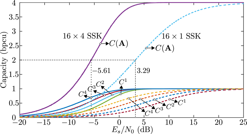
Figure 3: Different bit-level capacities for $16\times 1$ and $16\times 4$ SSK modulation.

III-C Polar Code Rate Allocation

To design the rates for the different levels of the multilevel polar code, we need to evaluate the overall SSK capacity and the corresponding $m_{a}$ bit-level capacities as given in Section III-A. We have computed the bit-level capacities by evaluating the expectation using Monte-Carlo simulation for a large number of frames for the received signal $\mathbf{y}$. The expectation averages the effect of the fast fading channels, resulting in the bit-level ergodic capacities. As an example, Fig. 3 shows the different bit-level ergodic capacities of $16\times 1$ and $16\times 4$ SSK modulations that are found using the Monte-Carlo simulation.

The bit-level MLC capacities are chosen for a particular information rate in bits per channel use (bpcu) of the overall SSK system using the capacity rule, which states that the rate of the $i$th component channel code should be $R_{i}\leq C^{i}$ for $1\leq i\leq m_{a}$. This design targets the overall rate for the length $m_{a}N$ polar code and the corresponding design signal-to-noise ratio (DSNR).

In the next step, we design the polar code of length $m_{a}N$ for a SISO Rayleigh fading channel using Tal-Vardy’s degrade transform and degrade merge methods for the DSNR [11], [10]. In the case of SSK, the effective channel is SIMO rather than SISO, and therefore this design is not capacity achieving, i.e., its capacity is less than that of MIMO-SSK channel; however, it provides a simple way to design the multilevel polar code for the SSK modulated system.

In the final step, we segregate the $m_{a}N$ length polar code into $m_{a}$ cascaded component polar codes according to the rates found using the MLC bit-level ergodic capacities as described in Section III-A.

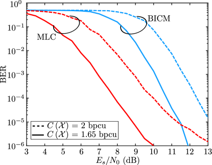
((a)) $16\times 1$ SSK system

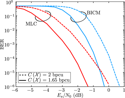
((b)) $16\times 4$ SSK system

Figure 4: Bit-error rate curves of BICM and MLC based SSK systems.

TABLE I: Rates and information bits size of multilevel polar codes

	$C\left(\mathbf{A}\right)$ (bpcu)
	$2$		$1.65$
SSK mode $(N_{T}\times N_{R})$	$16\times 1$	$16\times 4$	$16\times 1$	$16\times 4$
$E_{s}/N_{0}$ (dB)	$3.29$	$-5.61$	$1.5$	$-6.87$
$R_{1}$	$0.2738$	$0.3055$	$0.2037$	$0.2262$
$R_{2}$	$0.4143$	$0.4290$	$0.3232$	$0.3346$
$R_{3}$	$0.5856$	$0.5671$	$0.4809$	$0.4758$
$R_{4}$	$0.7323$	$0.6990$	$0.6456$	$0.6160$
$K_{1}$	$70$	$78$	$52$	$58$
$K_{2}$	$105$	$110$	$83$	$85$
$K_{3}$	$150$	$145$	$123$	$122$
$K_{4}$	$187$	$179$	$165$	$158$

IV Results and Discussion

We have designed polar codes of length $m_{a}N=1024$ for different SSK overall capacities. The rates and corresponding information bit sizes of the component polar codes are shown in Table I. Bit error rate (BER) simulations were run for a maximum of $5\times 10^{6}$ frames with a frame error limit of $100$ for all the BER curves.

To the best of the authors’ knowledge, multilevel polar codes have not previously been designed for use with SSK modulation. Therefore, the closest benchmark for performance comparison is with the bit-interleaved polar coded modulation. Fig. 4 shows the BER vs $E_{s}/N_{0}$ curves of BICM and MLC based SSK systems, where $E_{s}/N_{0}$ is the ratio of the transmitted energy per symbol to the noise power spectral density. For the $16\times 1$ SSK system shown in Fig. 4(a), the effective channel is single-input single output (SISO). For $C\left(\mathcal{X}\right)=2$ bpcu, the MLC based design outperforms BICM by $2.3$ dB at a BER of $10^{-4}$ which diminishes at high SNR $\left(\sim 11\right)$ dB and the two curves eventually intersect. On the other hand, the MLC system with $C\left(\mathcal{X}\right)=1.65$ bpcu outperforms BICM by $2.9$ dB at a BER$=10^{-4}$ and does not intersect until a BER of $10^{-6}$.

Fig. 4(b) shows the BER performance curve for a $16\times 4$ SSK system. The MLC based system outperforms BICM by a coding gain of $1$ dB and $1.5$ dB at a BER of $10^{-4}$ for $C\left(\mathcal{X}\right)=2$ and $1.65$ bpcu, respectively. Here, we again see the same trend that for high overall SSK capacity, the MLC BER curve approaches the BICM curve at high SNR. However, the coding gain is lower, as expected, as compared to the $16\times 1$ SSK system because at the receiver we have four separate received streams, i.e., the effective channel is SIMO.

V Conclusion

In this paper, we have designed multilevel polar codes for an SSK-modulated MIMO system. We used the capacity rule to evaluate the bit-level ergodic capacities of SSK modulation. As the spatial bits choose different transmitting channels, it is necessary to use Monte Carlo simulation to find the average bit-level capacities. As the effective channels are either SISO or SIMO, we base our polar code design on that for a SISO Rayleigh fading channel. This assumption is not capacity achieving but provides an easy way to design the multilevel polar coded system for a MIMO channel. BER simulation results show that the multilevel polar coded system with multilevel SSK modulation still provides considerable coding gain compared to the corresponding BICM system with SSK modulation.

This work can also be extended to design of multilevel polar codes for SM and generalized spatial modulation (GSM), which are suitable for attaining high spectral as well as energy efficiency.

Acknowlegment

This work was funded by the Irish Research Council under a Consolidator Laureate Award (grant no. IRCLA/2017/209).

Replace this box by an image with a width of 1 in and a height of 1.25 in!

Your Name All about you and the what your interests are.

Coauthor Same again for the co-author, but without photo

References

[1]
H. Imai and S. Hirakawa, “A new multilevel coding method using
error-correcting codes,” IEEE Transactions on Information Theory,
vol. 23, no. 3, pp. 371–377, 1977.
[2]
G. Ungerboeck and I. Csajka, “On improving data-link performance by
increasing channel alphabet and introducing sequence coding,” in IEEE
International Symposium on Information Theory, Ronneby, Sweden, June 1976.
[3]
G. Ungerboeck, “Channel coding with multilevel/phase signals,” IEEE
Transactions on Information Theory, vol. 28, no. 1, pp. 55–67, 1982.
[4]
E. Zehavi, “8-PSK trellis codes on Rayleigh channel,” in IEEE
Military Communications Conference, ’Bridging the Gap. Interoperability,
Survivability, Security’, Oct 1989, pp. 536–540 vol.2.
[5]
J. Huber and U. Wachsmann, “Capacities of equivalent channels in
multilevel coding schemes,” Electronics Letters, vol. 30, no. 7, pp.
557–558, 1994.
[6]
M. Seidl, A. Schenk, C. Stierstorfer, and J. B. Huber, “Aspects of
Polar-Coded Modulation,” in SCC 2013; 9th International ITG
Conference on Systems, Communication and Coding, 2013, pp. 1–6.
[7]
R. Mesleh, H. Haas, C. W. Ahn, and S. Yun, “Spatial Modulation - A
New Low Complexity Spectral Efficiency Enhancing Technique,”
in 2006 First International Conference on Communications and Networking
in China, 2006, pp. 1–5.
[8]
R. Y. Mesleh, H. Haas, S. Sinanovic, C. W. Ahn, and S. Yun, “Spatial
Modulation,” IEEE Transactions on Vehicular Technology, vol. 57,
no. 4, pp. 2228–2241, 2008.
[9]
J. Jeganathan, A. Ghrayeb, L. Szczecinski, and A. Ceron, “Space shift
keying modulation for mimo channels,” IEEE Transactions on Wireless
Communications, vol. 8, no. 7, pp. 3692–3703, 2009.
[10]
L. Liu and C. Ling, “Polar Codes and Polar Lattices for
Independent Fading Channels,” IEEE Transactions on
Communications, vol. 64, no. 12, pp. 4923–4935, 2016.
[11]
I. Tal and A. Vardy, “How to Construct Polar Codes,” IEEE
Transactions on Information Theory, vol. 59, no. 10, pp. 6562–6582, 2013.