Towards GW Calculations on Thousands of Atoms

Abstract

The $GW$ approximation of many-body perturbation theory is an accurate method for computing electron addition and removal energies of molecules and solids. In a canonical implementation, however, its computational cost is $\mathcal{O}(N^{4})$ in the system size $N$, which prohibits its application to many systems of interest. We present a full-frequency $GW$ algorithm in a Gaussian-type basis, whose computational cost scales with $N^{2}$ to $N^{3}$. The implementation is optimized for massively parallel execution on state-of-the-art supercomputers and is suitable for nanostructures and molecules in the gas, liquid or condensed phase, using either pseudopotentials or all electrons. We validate the accuracy of the algorithm on the $GW$100 molecular test set, finding mean absolute deviations of 35 meV for ionization potentials and 27 meV for electron affinities. Furthermore, we study the length-dependence of quasiparticle energies in armchair graphene nanoribbons of up to 1734 atoms in size, and compute the local density of states across a nanoscale heterojunction.

Present address: BASF SE, Carl-Bosch-Straße 38, D-67056 Ludwigshafen am Rhein, Germany Laboratory of Molecular Simulation, École Polytechnique Fédérale de Lausanne, Rue de l’Industrie 17, CH-1951 Sion, Switzerland

Electronic excitations in nanostructures and at complex interfaces play a decisive role in several key materials challenges, such as energy conversion ( 1) and digital electronics ( 2). The $GW$ approximation of many-body perturbation theory ( 3, 4) is a method devised for computing the energies of charged excitations, which involve the addition or removal of electrons. It accounts for the non-local, frequency-dependent screening of the interaction between electrons, which is particularly essential where materials vary over electronic length scales. The $GW$ spectra can be compared to photoemission spectroscopy and scanning-tunneling spectroscopy, and form the basis for the accurate prediction of optical spectra via the Bethe-Salpeter equation  ( 5). The good performance of the $GW$ approximation in predicting band structures of solids and, more recently, ionization potentials and electron affinities of molecules ( 6) has led to increasing interest from the chemistry community. However, the computational complexity of the canonical $GW$ algorithm ( 7, 8, 9, 10) is $\mathcal{O}(N^{4})$ in the system size $N$, with a substantial prefactor. This would prohibit the study of many systems of interest, such as solid-liquid interfaces ( 11), large metal complexes in solution ( 12), metal-organic frameworks ( 13), defect states ( 14) or $p$-$n$ junctions ( 15, 16) that require calculations on hundreds to thousands of atoms.

In recent years, substantial efforts have therefore been devoted to reducing the computational cost of $GW$ calculations. The prefactor has been tackled by avoiding the sum over empty states in the polarizability ( 17, 11, 18) as well as with a low-rank approximation of the dielectric matrix ( 11, 19). The size of the matrices involved can also be reduced by switching from the traditional plane-wave basis to smaller, localized basis sets ( 8, 7, 9, 20, 21), which are particularly suited for molecular systems ( 22, 23, 24, 25). Others have tackled the exponent: Foerster et al. ( 26) devised a cubic-scaling $GW$ algorithm in a Gaussian basis that exploits the locality of electronic interactions. The method has been applied to molecules with tens of atoms. Liu  et al. ( 27) implemented a variant of the cubic-scaling $GW$ space-time method ( 28), using a plane-wave basis, real-space grids and sophisticated minimax quadratures ( 27, 29) in imaginary time and frequency. Its linear scaling with the number of $k$-points is particularly promising for applications to large and numerically challenging periodic systems. Finally, Neuhauser et al. ( 30) reported a stochastic $GW$ algorithm which nominally enables linear scaling with system size and is straightforward to parallelize. The algorithm has been applied to a silicon nanocluster with one thousand atoms, but further exploration is needed to verify that stochastic $GW$ is a useful tool for more complex systems ( 31).

In this work, we present an efficient low-scaling $GW$ algorithm in a Gaussian basis that has been optimized for massively parallel execution on state-of-the-art supercomputers. In comparison to plane waves, the smaller size of the Gaussian basis together with the exploitation of sparsity in two- and three-index tensor operations increase performance while maintaining accuracy, as we demonstrate on the $GW$100 test set ( 32). The algorithm is suited for nanostructures and molecules in the gas, liquid or condensed phase and is implemented in version 5.0 of the open-source CP2K package ( 33).

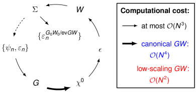
Figure 1: Sketch of $GW$ workflow. Regular arrows indicate operations of at most $\mathcal{O}(N^{3})$ computational complexity. The thick arrow is $\mathcal{O}(N^{4})$ in canonical $GW$ (blue) and $\mathcal{O}(N^{2})$ in low-scaling $GW$ (red). The dashed arrow corresponds to eigenvalue-selfconsistent $GW$ (ev$GW$). A detailed flowchart of the canonical and the low-scaling $GW$ algorithm can be found in the Supporting Information on page S2.

As sketched in Fig. 1, the $GW$ calculation starts from a set $\{\psi_{n},\varepsilon_{n}\}$ of single-particle orbitals $\psi_{n}$ and corresponding eigenenergies $\varepsilon_{n}$. Usually, these stem from a previous Kohn-Sham density functional theory (DFT) calculation, but other starting points, such as Hartree-Fock and hybrid functionals, are also available.

The orbitals are expanded in the primary Gaussian-type orbitals (GTOs) $\{\phi_{\mu}\}$

$$\psi_{n}(\mathbf{r})=\sum_{\mu}C_{n\mu}\phi_{\mu}(\mathbf{r})$$ (1)

using the molecular orbital (MO) coefficients $C_{n\mu}$.

Following the $GW$ space-time method, we proceed to computing the time-ordered single-particle Green’s function $G(i\tau)$ in imaginary time:

$$\begin{split}G_{\mu\nu}(i\tau)=\left\{\begin{array}[]{ll}i\sum\limits_{n}^{\text{occ}}C_{n\mu}C_{n\nu}\exp(\varepsilon_{n}\tau)\,,&\tau>0\,,\\[5.0pt] -i\sum\limits_{n}^{\text{virt}}C_{n\mu}C_{n\nu}\exp(\varepsilon_{n}\tau)\,,&\tau<0\,.\end{array}\right.\end{split}$$ (2)

A key step in the algorithm is computing the irreducible polarizability $\chi^{0}(i\tau)\hskip 1.69998pt{=}\hskip 1.69998pt-iG(i\tau)G(-i\tau)$. ( 28) Building on previous work ( 34), $\chi^{0}$ is obtained in an auxiliary Gaussian basis $\{\varphi_{P}\}$ ( 35, 36, 37) that is designed to span the product space $\{\psi_{i}\}\hskip 1.19995pt{\otimes}\hskip 1.19995pt\{\psi_{a}\}$ of occupied and unoccupied orbitals, and is typically two to three times larger than the corresponding primary basis $\{\phi_{\mu}\}$. The matrix ${\chi}^{0}_{PQ}(i\tau)\hskip 1.69998pt{=}\hskip 1.69998pt\braket{\varphi_{P}}{\chi^{0}(i\tau)}{\varphi_{Q}}$ is calculated as

$$\begin{split}{\chi}^{0}_{PQ}(i\tau)=-i&\sum\limits_{\mu\sigma}\sum\limits_{\lambda}(\lambda\sigma P)G_{\mu\lambda}(i\tau)\\[5.0pt] &\times\sum\limits_{\nu}(\mu\nu Q)G_{\nu\sigma}(-i\tau)\,,\end{split}$$ (3)

where the three-center overlap tensors

$$(\nu\mu P)={\int}d\mathbf{r}\;\phi_{\nu}(\mathbf{r})\phi_{\mu}(\mathbf{r})\varphi_{P}(\mathbf{r})$$ (4)

are computed analytically ( 34).

Since the overlap tensors $(\mu\nu P)$ vanish unless the GTOs $\phi_{\mu}$, $\phi_{\nu}$ and $\varphi_{P}$ are centered on nearby atoms, their size grows only linearly with the system size $N$. The computational cost of Eq. (3) is therefore $\mathcal{O}(N^{2})$ blackwithout the requirement of sparse density matrices or additional localization techniques. The overlap tensor in Eq. (4) can be understood as deriving from the resolution of the identity (RI) with the overlap metric black(RI-SVS) ( 38, 39, 40). We note that the popular RI with the Coulomb metric black(RI-V) ( 38) blackconverges faster with the size of the RI basis, but does not lead to sparsity in (4) and would thus provide no advantage over the canonical implementation (see supporting information).

Although the cost of the matrix-matrix multiplication in Eq. (2) and all following matrix operations in Eqs. (5), (7), (8), (9) scale cubically with system size, Eq. (3) remains the computational bottleneck even for the largest systems addressed in this work. Therefore, the computation of the polarizability from Eq. (3) has been optimized for massive parallelism ( 34) using the DBCSR library for sparse matrix-matrix multiplications ( 41).

We proceed by including the non-orthogonality of $\{\varphi_{P}\}$ in $\boldsymbol{\tilde{\chi}}^{0}(i\tau)$,

$$\boldsymbol{\tilde{\chi}}^{0}(i\tau)=\mathbf{S}^{-1}\boldsymbol{\chi}^{0}(i\tau)\mathbf{S}^{-1}$$ (5)

via the overlap matrix

$$S_{PQ}\hskip 1.69998pt{=}\hskip 1.69998pt{\int}d\mathbf{r}\,\varphi_{P}(\mathbf{r})\varphi_{Q}(\mathbf{r})\,.$$ (6)

Following the route of the $GW$ space-time method ( 28), the polarizability $\boldsymbol{\chi}^{0}(i\tau)$ is transformed to imaginary frequencies via a cosine transform on the minimax grid, ( 27) and the symmetric dielectric function $\epsilon(i\omega)$ is computed by ( 42)

$$\boldsymbol{\epsilon}(i\omega)=\mathbf{1}-\mathbf{L}^{\text{T}}\boldsymbol{\tilde{\chi}}^{0}(i\omega)\mathbf{L}$$ (7)

where $\mathbf{L}$ denotes the Cholesky decomposition of the Coulomb matrix $\mathbf{V}$,

$$\mathbf{V}=\mathbf{L}\mathbf{L}^{\text{T}}\,,\hskip 10.00002ptV_{PQ}={\int}d\mathbf{r}\hskip 0.50003ptd\mathbf{r}^{\prime}\,\varphi_{P}(\mathbf{r})\,\frac{1}{|\mathbf{r}-\mathbf{r^{\prime}}|}\,\varphi_{Q}(\mathbf{r}^{\prime})\,.$$ (8)

For molecules, the Coulomb matrix is computed analytically ( 43) and for periodic systems numerically by Ewald summation ( 44), as commonly used in wavefunction correlation methods ( 45, 46, 47). We note that the algorithm supports both aperiodic and periodic simulation cells in the $\Gamma$-only approach ( 42). For periodicity in three dimensions, a correction scheme is available to accelerate the convergence with supercell size ( 42).

The screened interaction $W(i\omega)=\epsilon^{-1}(i\omega)V=V\hskip 1.69998pt{+}\hskip 1.69998ptW^{c}(i\omega)$ is split into the bare Coulomb interaction and the correlation contribution, and the latter is obtained as ( 42)

$$\mathbf{W}^{\text{c}}(i\omega)=\mathbf{L}\left[\boldsymbol{\epsilon}^{-1}(i\omega)-\mathbf{1}\right]\mathbf{L}^{\text{T}}\,,$$ (9)

where the symmetric, positive definite $\boldsymbol{\epsilon}(i\omega)$ is inverted efficiently by Cholesky decomposition. A cosine transform brings $W^{c}(i\omega)$ back to imaginary time.

This completes the ingredients for the $GW$ self-energy $\Sigma(i\tau)\hskip 1.69998pt{=}\hskip 1.69998ptiG(i\tau)W(i\tau)\hskip 1.69998pt{=:}\hskip 1.69998pt\Sigma^{\text{x}}\hskip 1.69998pt{+}\hskip 1.69998pt\Sigma^{\text{c}}(i\tau)$. In the following, we restrict the treatment to $GW$ schemes without orbital updates, such as $G_{0}W_{0}$ and eigenvalue self-consistent $GW$ (ev$GW$). Computing the quasiparticle energies for $N_{GW}$ orbitals $\psi_{n}$ then only requires the $N_{GW}$ corresponding diagonal matrix elements $\Sigma_{n}(i\tau)\hskip 1.69998pt{=}\hskip 1.69998pt\braket{\psi_{n}}{\Sigma(i\tau)}{\psi_{n}}$. For reasons of computational efficiency, we compute the diagonal elements directly, yielding the correlation self-energy

$$\Sigma_{n}^{\text{c}}(i\tau)=i\sum_{\nu P}\sum_{\mu}G_{\mu\nu}(i\tau)(n\mu P)\sum_{Q}\tilde{W}^{\text{c}}_{PQ}(i\tau)(Q\nu n)\,,$$ (10)

where $\tilde{\mathbf{W}}^{\text{c}}(i\tau)\hskip 1.69998pt{=}\hskip 1.69998pt\mathbf{S}^{-1}\mathbf{W}^{\text{c}}(i\tau)\mathbf{S}^{-1}$, and the static exchange self-energy

$$\Sigma^{\text{x}}_{n}=-\sum_{\nu P}\sum_{\mu}D_{\mu\nu}(n\mu P)\sum_{Q}\tilde{V}_{PQ}(Q\nu n)\,,$$ (11)

where $D_{\mu\nu}\hskip 1.69998pt{=}\hskip 1.69998pt\sum_{n}^{\text{occ}}C_{n\mu}C_{n\nu}$ and $\tilde{\mathbf{V}}=\mathbf{S}^{-1}\mathbf{V}\mathbf{S}^{-1}$.

The computational complexity of Eq. (10) and (11) is $\mathcal{O}(N_{GW}N^{2})$, since $(n\mu P)\hskip 1.69998pt{=}\hskip 1.69998pt{\sum_{\nu}}C_{n\nu}(\nu\mu P)$ vanishes if $\phi_{\mu}$ and $\varphi_{P}$ are centered on atoms far apart from each other, introducing sparsity.

In order to compute quasiparticle energies, $\Sigma^{\text{c}}_{n}(i\tau)$ is transformed to imaginary frequencies by a sine and cosine transform. ( 27) It is then evaluated on the real frequency axis $\Sigma^{\text{c}}_{n}(\varepsilon)$ by analytic continuation using a Padé interpolant of $\Sigma^{\text{c}}_{n}(i\omega)$ ( 32, 27). The $G_{0}W_{0}$ quasiparticle energies $\varepsilon_{n}^{G_{0}W_{0}}$ are obtained by replacing the DFT exchange-correlation contribution $v^{\text{xc}}_{n}$ with the self-energy,

$$\varepsilon_{n}^{G_{0}W_{0}}=\varepsilon_{n}-v^{\text{xc}}_{n}+\Sigma^{\text{x}}_{n}+\text{Re}\,\Sigma^{\text{c}}_{n}(\varepsilon_{n}^{G_{0}W_{0}})$$ (12)

and solving Eq. (12) iteratively for $\varepsilon_{n}^{G_{0}W_{0}}$ via Newton-Raphson. For eigenvalue-selfconsistent $GW$, the quasiparticle energies then replace the DFT levels in Eqs. (2) and the $GW$ cycle of Fig. 1 is repeated until self-consistency in the quasiparticle energies $\varepsilon_{n}^{\text{ev{GW}}}$ is achieved.

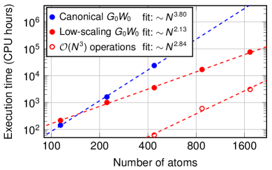
Figure 2: Scaling of $G_{0}W_{0}$ execution time with number of atoms. The canonical algorithm ( 9) (blue dots) is compared against the low-scaling algorithm (red dots) and its fraction of cubically-scaling operations (red circles). Dashed lines are two-parameters least-squares fits of prefactor and exponent. The systems under study are graphene nanoribbons as shown in Fig. 3. For the largest system containing 1734 atoms, we compute 2883 occupied molecular orbitals and 30195 virtual ones, using 80940 auxiliary basis functions. This calculation was performed on 14400 CPUs on a CRAY XC40 machine.

Fig. 2 illustrates how the computational cost of the algorithm scales with the number of atoms $N$ for a technologically relevant test system of graphene nanoribbons, which is discussed in more detail below. The total execution time of the canonical $G_{0}W_{0}$@PBE implementation ( 9) (blue) scales with $N^{3.8}$, and constraints in computation time and memory prohibit us from going beyond 500 atoms. blackThe low-scaling algorithm (red) becomes superior between 100 and 200 atoms, is already a factor of 8 faster at 438 atoms than the canonical implementation, and allows to reach much larger system sizes on the same computer architecture (1734 atoms and 5766 electrons in this example).

We stress that the cost of the low-scaling algorithm scales like $N^{2.1}$ with the number of atoms $N$ in the range considered here, since the cubic-scaling steps (red circles) have a much smaller prefactor than the $\mathcal{O}(N^{2})$ evaluation of Eq. (3) blackinvolving sparse tensor operations. blackIn this regime, we expect the algorithm to be particularly efficient for low-dimensional systems, such as 2d materials or 1d polymers and wires, as well as for systems with a local electronic structure, such as molecules in solution, which give rise to sparse density matrices and Green’s functions ( 48). blackFor very large systems, the cubic-scaling steps will dominate and sparsity becomes irrelevant. By extrapolating the data shown in Fig. 2, we estimate the cross-over from quadratically-dominated to cubically-dominated to occur at $\approx$ $3\hskip 1.30005pt{\cdot}\hskip 1.30005pt10^{4}$ atoms ($\approx$ $10^{5}$ electrons) for the systems under study. blackFor very small systems, all three-center integrals have to be retained and the larger RI-SVS basis puts the low-scaling $GW$ at a slight disadvantage compared to the canonical algorithm using RI-V.

The accuracy of the low-scaling $GW$ algorithm is validated on the $GW$100 set by van Setten et al. ( 32) We compute the energies of the highest occupied molecular orbital (HOMO), or ionization potential, and the lowest unoccupied molecular orbital (LUMO), or electron affinity, at the $G_{0}W_{0}$@PBE level for all molecules in the set. All values are reported in the Supporting Information on pages S3/S4 and compared to reference values from FHI-aims ( 32, 7), an all-electron code using numerical, atom-centered basis functions. We find that HOMO energies match within 30 meV for 74 out of 100 molecules, while LUMO energies match within 30 meV for 87 molecules.

For comparison, we note that HOMO energies from FHI-aims and VASP ( 27), a plane-wave code implementing the projector augmented wave method ( 49), have a mean absolute deviation (MAD) of 60 meV on a subset of $GW$100 ( 50), while we find a MAD of 35  meV between FHI-aims and our algorithm (on $GW$100 excluding BN, O₃, BeO, MgO, CuCN and Ne). We conclude that our implementation is suitably accurate and continue by discussing its application to large systems.

We start by studying anthenes, graphene nanoribbons (GNRs) of seven carbon atoms width, as depicted in Fig. 3 (a). Recent advances in on-surface chemistry have enabled the bottom-up fabrication of these GNRs with atomic precision ( 51), and their electronic structure has been investigated in detail by scanning tunneling spectroscopy ( 52, 53). For these particular GNRs, HOMO and LUMO are found to be localized at the zigzag edges of the ribbons, as depicted in Fig. 3 (a), while the remaining frontier orbitals delocalize along the ribbon. One therefore distinguishes the zigzag gap $\Delta_{\text{zz}}$ between edge-localized HOMO and LUMO states, and the armchair gap $\Delta_{\text{AC}}$ between the delocalized HOMO-1 and LUMO+1, as sketched in Fig. 3 (b). Since only the delocalized states are available for charge transport along the ribbon, $\Delta_{\text{AC}}$ is also termed the transport gap. We compute $\Delta_{\text{zz}}$ and $\Delta_{\text{AC}}$ for anthenes containing up to 1734 atoms, see Fig. 3 (c) and (d).

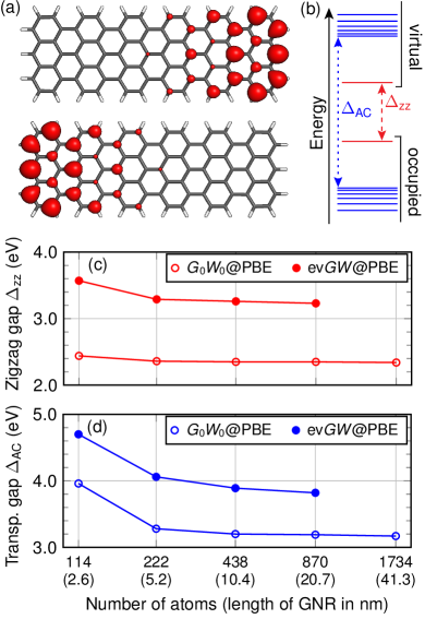
Figure 3: (a) Molecular geometry of 6-anthene together with the zigzag edge states obtained from DFT. blackAll edge carbon atoms are passivated by a single hydrogen atom. Shown in red are isosurfaces of constant probability density for the HOMO (top) and LUMO (bottom) of the spin-up channel. (b) Sketch illustrating the corresponding spectrum with the HOMO$-$LUMO gap $\Delta_{\text{zz}}$ between zigzag (zz) states and the transport gap $\Delta_{\text{AC}}$ (HOMO-1$-$LUMO+1) between bulk states. (c) Zigzag gap $\Delta_{\text{zz}}$ and (d) transport gap $\Delta_{\text{AC}}$ of anthenes with a horizontal length from 2.6 nm to 41.3 nm.

As expected from their highly localized nature, and in agreement with previous work ( 53), the zigzag gap converges quickly with length. First, we note that the converged $G_{0}W_{0}$@PBE value of $\Delta_{\text{zz}}\hskip 1.69998pt{=}\hskip 1.69998pt2.4\,$eV is significantly lower than the 2.8 eV reported in Ref. 53, where the frequency-dependence of the polarizability was approximated by a plasmon-pole model. This is in line with findings for molecules in $GW$100 ( 32) and indicates that plasmon-pole models should be avoided in future studies of localized states in GNRs. Secondly, self-consistency in the eigenvalues leads to a substantial increase of the gap to 3.2 eV. This observation blackis easily understood by considering that the tiny PBE Kohn-Sham gap of 0.6 eV gives rise to a strong screening of this localized state in the interaction $W_{0}$ that is suppressed by the larger $GW$ gap in subsequent self-consistency iterations. blackTechniques for improving the DFT starting point include the use of hybrid density functionals with adequate fractions of Hartree-Fock exchange  ( 54, 55).

The low-scaling algorithm also allows us to study the convergence of the transport gap with GNR length, which requires significantly longer GNRs due to the delocalized nature of the involved electronic states. As shown in Fig. 3 (d), the transport gap saturates at a value of $\Delta_{\text{AC}}\hskip 1.69998pt{=}\hskip 1.69998pt3.2\,$eV ($G_{0}W_{0}@$PBE). Again, this value is significantly smaller than the value of 3.8 eV reported in early $G_{0}W_{0}$@LDA calculations ( 56) using periodic boundary conditions and a plasmon-pole model. The effect of eigenvalue-selfconsistency, while still substantial, is smaller for the transport gap, leading to a ev$GW$@PBE value of 3.8 eV.

In order to enable comparison with experiments ( 57), where the GNRs are physisorbed on the highly polarizable Au(111) surface, we include the effect of the screening by the substrate via an image charge model devised specifically for the case of GNRs on noble metal surfaces ( 58). The gap of the pristine GNR reduces by $\Delta_{\text{IC}}\approx 1.3\,$eV to $\approx 2.5$ eV in good agreement with previous experimental and theoretical work ( 52, 53, 58).

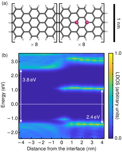
Figure 4: Graphene nanoribbon heterojunction. (a) Atomistic model including 870 atoms (boron dopants shown in purple). (b) Local density of states across the junction based on ev$GW$@PBE eigenvalues, with Gaussian broadening of 0.1 eV and integrated over the plane orthogonal to the GNR axis. The energy zero was chosen as the center of the gap.

Next, we turn our attention to heterostructures between doped and undoped GNRs that have recently been demonstrated via on-surface synthesis ( 16, 15, 57). The controlled modulation of the band structure and charge carrier concentration through doping, as well as the synthesis of atomically precise heterojunctions are crucial milestones on the path towards graphene nanoribbon electronics. While many-body perturbation theory in the $GW$ approximation is well-equipped to capture the level alignment, energy gaps and local density of states (LDOS) across such interfaces, the long range of the Coulomb interaction can make it necessary to treat large numbers of atoms in order to obtain converged results.

Fig. 4 (a) depicts an interface between a pristine GNR and its boron-doped variant, as blackrealized experimentally via bottom-up synthesis in Ref. 15. We perform ev$GW$@PBE calculations for the heterojunction containing 870 atoms, which converges the gap to $\approx$ 0.1 eV, cf. Fig. 3 (d). The LDOS at the interface between pristine and doped side is shown in Fig. 4 (b). For the bulk gap on the pristine side, we recover the value of 3.8 eV from Fig. 3 (d), while blackthe empty $p$ orbitals of B give rise to a weakly dispersing acceptor band ( 15), yielding a lower band gap of 2.4 eV for the doped GNR. The LDOS also reveals information specific to the interface: the valence band maxima of the pristine and doped GNR align, blackmaking this a type-I (straddling gap) heterojunction. Despite the perfect lattice match, an interface state appears close to the Fermi edge ( 57), which can blackintroduce backscattering and thus strongly affect the current response of the heterojunction at low bias voltages ( 59). As pointed out by Cao et al. ( 60), the presence this interface state can be deduced from topological arguments, since the interface is one between a one-dimensional topological insulator ($Z_{2}=1$) on the left, and a trivial insulator ($Z_{2}=0)$ on the right.

In summary, we have presented an efficient algorithm for computing quasiparticle energies in the $GW$ approximation, requiring $\mathcal{O}(N^{3})$ operations and $\mathcal{O}(N^{2})$ memory. The method is a reformulation of the $GW$ space-time method ( 28) in a Gaussian basis using sparse linear algebra and minimax grids ( 27) for imaginary time and frequency. Both $G_{0}W_{0}$ and eigenvalue-selfconsistent $GW$ are supported, using either periodic or aperiodic boundary conditions. We have implemented the algorithm in version 5.0 of the open-source CP2K package ( 33) and benchmarked its accuracy on the complete $GW$100 set of molecules, finding good agreement with reference implementations. The scalability of the algorithm was demonstrated by computing quasiparticle energies of graphene nanoribbons containing up to 1734 atoms and the spatially resolved local density of states of a graphene nanoribbon heterojunction. By reducing the cost of computing accurate electron removal and addition energies in nanostructures, molecules and their composites, our work provides yet another stepping stone on the path towards in silico materials design.

Computational Methods

For the $GW$100 benchmark set ( 32), we solve the all-electron Kohn-Sham (KS) equations in the Gaussian and augmented plane waves scheme (GAPW) ( 61) as implemented in CP2K ( 33). The molecular orbitals are expanded in a def2-QZVP Gaussian-type basis ( 32) [Eq. (1)], while $GW$ quantities are expanded in a blackcc-pV5Z-RI auxiliary basis $\{\varphi_{P}\}$ blacktaken from the EMSL database ( 37). blackFor the 17 elements from K to Ne not covered by the cc-pV5Z-RI basis, we constructed a large RI basis containing 124 sets up to I functions. 12-point minimax grids were used in imaginary time and frequency. blackFor the analytic continuation, we construct the Padé approximant on the subset of imaginary frequency points in the interval $i[0,\pm 10\,\text{eV}]$, where $+/-$ applies to virtual/occupied MOs.

For the GNRs, we solve the singlet open-shell KS equations in the Gaussian and plane waves scheme (GPW) ( 62) using Goedecker-Teter-Hutter pseudopotentials ( 63). The molecular orbitals are expanded in an aug-DZVP Gaussian-type basis which converges the HOMO-LUMO gap within a few tens of meV, see also Ref.  9. As the auxiliary basis, we employ the corresponding RI-aug-DZVP basis from Ref.  9 which has been generated by optimizing the RI-MP2 energy to match the MP2 energy ( 36, 35). For the $GW$ calculations, atom blocks of basis functions with a Frobenius norm lower than $10^{-11}$ were filtered ( 41) to make sparse tensor operations [Eqs. (3) and  (10)] efficient. This filter threshold is low enough to affect the $G_{0}W_{0}$ HOMO-LUMO gap of the 6-anthene by less than $0.01$ eV. blackWe note that using the same filter threshold for the $GW$100 set results in no filtering at all due to the small size of the molecules, i.e. the GNRs and the molecules are treated equally in this respect. blackFurther information on the choice of the filter threshold can be found in the Supporting Information. Again, we use 12-point minimax grids in time and frequency. Fig. 4 (b) was produced by projecting the LDOS onto the atomic orbitals of the GNR and summing over all nine atoms in a vertical line. In this way, the LDOS is integrated over the plane perpendicular to the ribbon axis.

An exemplary, annotated input file is provided in the Supporting Information on page S6.

Supporting Information

A detailed comparison between low-scaling and canonical $\mathcal{O}(N^{4})$-scaling $GW$ in a Gaussian basis including a discussion of the resolution of the identity is given; all values for the $GW$100 test set, a discussion on choosing filter parameters for sparse tensor operations, an exemplary input file together with basis sets and a discussion on the basis set convergence are reported. This material is available free of charge via the Internet at http:// pubs.acs.org.

References

- Ping et al. 2013 Ping, Y.; Rocca, D.; Galli, G. Electronic excitations in light absorbers for photoelectrochemical energy conversion: first principles calculations based on many body perturbation theory. Chem. Soc. Rev. 2013, 42, 2437–2469
- Schwierz 2013 Schwierz, F. Graphene transistors: status, prospects, and problems. Proc. IEEE 2013, 101, 1567–1584
- Hedin 1965 Hedin, L. New Method for Calculating the One-Particle Green’s Function with Application to the Electron-Gas Problem. Phys. Rev. 1965, 139, A796–A823
- Onida et al. 2002 Onida, G.; Reining, L.; Rubio, A. Electronic excitations: density-functional versus many-body Green’s-function approaches. Rev. Mod. Phys. 2002, 74, 601
- Jacquemin et al. 2017 Jacquemin, D.; Duchemin, I.; Blase, X. Is the Bethe-Salpeter Formalism Accurate for Excitation Energies? Comparisons with TD-DFT, CASPT2, and EOM-CCSD. J. Phys. Chem. Lett. 2017, 8, 1524–1529
- Marom 2017 Marom, N. Accurate description of the electronic structure of organic semiconductors by GW methods. J. Phys. Condens. Matter 2017, 29, 103003
- Ren et al. 2012 Ren, X.; Rinke, P.; Blum, V.; Wieferink, J.; Tkatchenko, A.; Sanfilippo, A.; Reuter, K.; Scheffler, M. Resolution-of-identity approach to Hartree-Fock, hybrid density functionals, RPA, MP2 and GW with numeric atom-centered orbital basis functions. New J. Phys. 2012, 14, 053020
- Blase et al. 2011 Blase, X.; Attaccalite, C.; Olevano, V. First-principles calculations for fullerenes, porphyrins, phtalocyanine, and other molecules of interest for organic photovoltaic applications. Phys. Rev. B 2011, 83, 115103
- Wilhelm et al. 2016 Wilhelm, J.; Del Ben, M.; Hutter, J. GW in the Gaussian and Plane Waves Scheme with Application to Linear Acenes. J. Chem. Theory Comput. 2016, 12, 3623–3635
- Deslippe et al. 2012 Deslippe, J.; Samsonidze, G.; Strubbe, D. A.; Jain, M.; Cohen, M. L.; Louie, S. G. BerkeleyGW: A massively parallel computer package for the calculation of the quasiparticle and optical properties of materials and nanostructures. Comput. Phys. Commun. 2012, 183, 1269–1289
- Govoni and Galli 2015 Govoni, M.; Galli, G. Large Scale GW calculations. J. Chem. Theory Comput. 2015, 11, 2680–2696
- Evangelisti et al. 2013 Evangelisti, F.; Güttinger, R.; Moré, R.; Luber, S.; Patzke, G. R. Closer to Photosystem II: A Co4O4 Cubane Catalyst with Flexible Ligand Architecture. J. Am. Chem. Soc. 2013, 135, 18734–18737
- Sun et al. 2016 Sun, L.; Campbell, M. G.; Dincă, M. Electrically Conductive Porous Metal-Organic Frameworks. Angew. Chem. Int. Ed. 2016, 55, 3566–3579
- Walz et al. 2014 Walz, M.; Wilhelm, J.; Evers, F. Current Patterns and Orbital Magnetism in Mesoscopic dc Transport. Phys. Rev. Lett. 2014, 113, 136602
- Cloke et al. 2015 Cloke, R. R.; Marangoni, T.; Nguyen, G. D.; Joshi, T.; Rizzo, D. J.; Bronner, C.; Cao, T.; Louie, S. G.; Crommie, M. F.; Fischer, F. R. Site-Specific Substitutional Boron Doping of Semiconducting Armchair Graphene Nanoribbons. J. Am. Chem. Soc. 2015, 137, 8872–8875
- Cai et al. 2014 Cai, J.; Pignedoli, C. A.; Talirz, L.; Ruffieux, P.; Söde, H.; Liang, L.; Meunier, V.; Berger, R.; Li, R.; Feng, X., et al. Graphene nanoribbon heterojunctions. Nat. Nanotechnol. 2014, 9, 896–900
- Umari et al. 2010 Umari, P.; Stenuit, G.; Baroni, S. GW quasiparticle spectra from occupied states only. Phys. Rev. B 2010, 81, 115104
- Bruneval 2016 Bruneval, F. Optimized virtual orbital subspace for faster GW calculations in localized basis. J. Chem. Phys. 2016, 145, 234110
- Giustino et al. 2010 Giustino, F.; Cohen, M. L.; Louie, S. G. GW method with the self-consistent Sternheimer equation. Phys. Rev. B 2010, 81, 115105
- van Setten et al. 2013 van Setten, M. J.; Weigend, F.; Evers, F. The GW-Method for Quantum Chemistry Applications: Theory and Implementation. J. Chem. Theory Comput. 2013, 9, 232–246
- Bruneval et al. 2016 Bruneval, F.; Rangel, T.; Hamed, S. M.; Shao, M.; Yang, C.; Neaton, J. B. molgw 1: Many-body perturbation theory software for atoms, molecules, and clusters. Comp. Phys. Comm. 2016, 208, 149–161
- Bruneval and Marques 2013 Bruneval, F.; Marques, M. A. L. Benchmarking the Starting Points of the GW Approximation for Molecules. J. Chem. Theory Comput. 2013, 9, 324–329
- Körbel et al. 2014 Körbel, S.; Boulanger, P.; Duchemin, I.; Blase, X.; Marques, M. A. L.; Botti, S. Benchmark Many-Body GW and Bethe–Salpeter Calculations for Small Transition Metal Molecules. J. Chem. Theory Comput. 2014, 10, 3934–3943
- Knight et al. 2016 Knight, J. W.; Wang, X.; Gallandi, L.; Dolgounitcheva, O.; Ren, X.; Ortiz, J. V.; Rinke, P.; Körzdörfer, T.; Marom, N. Accurate ionization potentials and electron affinities of acceptor molecules III: a benchmark of GW methods. J. Chem. Theory Comput. 2016, 12, 615–626
- Rangel et al. 2016 Rangel, T.; Hamed, S. M.; Bruneval, F.; Neaton, J. B. Evaluating the GW Approximation with CCSD(T) for Charged Excitations Across the Oligoacenes. J. Chem. Theory Comput. 2016, 12, 2834–2842
- Foerster et al. 2011 Foerster, D.; Koval, P.; Sánchez-Portal, D. An implementation of Hedin’s approximation for molecules. J. Chem. Phys. 2011, 135, 074105
- Liu et al. 2016 Liu, P.; Kaltak, M.; Klimeš, J.; Kresse, G. Cubic scaling : Towards fast quasiparticle calculations. Phys. Rev. B 2016, 94, 165109
- Rojas et al. 1995 Rojas, H. N.; Godby, R. W.; Needs, R. J. Space-Time Method for Ab Initio Calculations of Self-Energies and Dielectric Response Functions of Solids. Phys. Rev. Lett. 1995, 74, 1827
- Kaltak et al. 2014 Kaltak, M.; Klimeš, J.; Kresse, G. Low Scaling Algorithms for the Random Phase Approximation: Imaginary Time and Laplace Transforms. J. Chem. Theory Comput. 2014, 10, 2498–2507
- Neuhauser et al. 2014 Neuhauser, D.; Gao, Y.; Arntsen, C.; Karshenas, C.; Rabani, E.; Baer, R. Breaking the Theoretical Scaling Limit for Predicting Quasiparticle Energies: The Stochastic Approach. Phys. Rev. Lett. 2014, 113, 076402
- Vlček et al. 2017 Vlček, V.; Rabani, E.; Neuhauser, D.; Baer, R. Stochastic GW Calculations for Molecules. J. Chem. Theory Comput. 2017, 13, 4997–5003
- van Setten et al. 2015 van Setten, M. J.; Caruso, F.; Sharifzadeh, S.; Ren, X.; Scheffler, M.; Liu, F.; Lischner, J.; Lin, L.; Deslippe, J. R.; Louie, S. G.; Yang, C.; Weigend, F.; Neaton, J. B.; Evers, F.; Rinke, P. 100: Benchmarking for Molecular Systems. J. Chem. Theory Comput. 2015, 11, 5665–5687
- Hutter et al. 2014 Hutter, J.; Iannuzzi, M.; Schiffmann, F.; VandeVondele, J. cp2k: atomistic simulations of condensed matter systems. WIREs Comput. Mol. Sci. 2014, 4, 15–25
- Wilhelm et al. 2016 Wilhelm, J.; Seewald, P.; Del Ben, M.; Hutter, J. Large-Scale Cubic-Scaling Random Phase Approximation Correlation Energy Calculations Using a Gaussian Basis. J. Chem. Theory Comput. 2016, 12, 5851–5859
- Weigend et al. 1998 Weigend, F.; Häser, M.; Patzelt, H.; Ahlrichs, R. RI-MP2: optimized auxiliary basis sets and demonstration of efficiency. Chem. Phys. Lett. 1998, 294, 143–152
- Del Ben et al. 2013 Del Ben, M.; Hutter, J.; VandeVondele, J. Electron Correlation in the Condensed Phase from a Resolution of Identity Approach Based on the Gaussian and Plane Waves Scheme. J. Chem. Theory Comput. 2013, 9, 2654–2671
- Schuchardt et al. 2007 Schuchardt, K. L.; Didier, B. T.; Elsethagen, T.; Sun, L.; Gurumoorthi, V.; Chase, J.; Li, J.; Windus, T. L. Basis Set Exchange: A Community Database for Computational Sciences. J. Chem. Inf. Model. 2007, 47, 1045–1052
- Vahtras et al. 1993 Vahtras, O.; Almlöf, J.; Feyereisen, M. Integral approximations for LCAO-SCF calculations. Chem. Phys. Lett. 1993, 213, 514–518
- Schurkus and Ochsenfeld 2016 Schurkus, H. F.; Ochsenfeld, C. Communication: An effective linear-scaling atomic-orbital reformulation of the random-phase approximation using a contracted double-Laplace transformation. J. Chem. Phys. 2016, 144, 031101
- Duchemin et al. 2017 Duchemin, I.; Li, J.; Blase, X. Hybrid and Constrained Resolution-of-Identity Techniques for Coulomb Integrals. J. Chem. Theory Comput. 2017, 13, 1199–1208
- Borštnik et al. 2014 Borštnik, U.; VandeVondele, J.; Weber, V.; Hutter, J. Sparse matrix multiplication: The distributed block-compressed sparse row library. Parallel Comput. 2014, 40, 47–58
- Wilhelm and Hutter 2017 Wilhelm, J.; Hutter, J. Periodic calculations in the Gaussian and plane-waves scheme. Phys. Rev. B 2017, 95, 235123
- Golze et al. 2017 Golze, D.; Benedikter, N.; Iannuzzi, M.; Wilhelm, J.; Hutter, J. Fast evaluation of solid harmonic Gaussian integrals for local resolution-of-the-identity methods and range-separated hybrid functionals. J. Chem. Phys. 2017, 146, 034105
- Ewald 1921 Ewald, P. P. Die Berechnung optischer und elektrostatischer Gitterpotentiale. Ann. Phys. 1921, 369, 253–287
- Del Ben et al. 2015 Del Ben, M.; Hutter, J.; VandeVondele, J. Forces and stress in second order Møller-Plesset perturbation theory for condensed phase systems within the resolution-of-identity Gaussian and plane waves approach. J. Chem. Phys. 2015, 143, 102803
- Rybkin and VandeVondele 2016 Rybkin, V. V.; VandeVondele, J. Spin-Unrestricted Second-Order Møller-Plesset (MP2) Forces for the Condensed Phase: From Molecular Radicals to F-Centers in Solids. J. Chem. Theory Comput. 2016, 12, 2214–2223
- Del Ben et al. 2015 Del Ben, M.; Schütt, O.; Wentz, T.; Messmer, P.; Hutter, J.; VandeVondele, J. Enabling simulation at the fifth rung of DFT: Large scale RPA calculations with excellent time to solution. Comput. Phys. Commun. 2015, 187, 120–129
- Baer and Head-Gordon 1997 Baer, R.; Head-Gordon, M. Sparsity of the Density Matrix in Kohn-Sham Density Functional Theory and an Assessment of Linear System-Size Scaling Methods. Phys. Rev. Lett. 1997, 79, 3962–3965
- Blöchl 1994 Blöchl, P. E. Projector augmented-wave method. Phys. Rev. B 1994, 50, 17953–17979
- Maggio et al. 2017 Maggio, E.; Liu, P.; van Setten, M. J.; Kresse, G. GW100: A Plane Wave Perspective for Small Molecules. J. Chem. Theory Comput. 2017, 13, 635–648
- Cai et al. 2010 Cai, J.; Ruffieux, P.; Jaafar, R.; Bieri, M.; Braun, T.; Blankenburg, S.; Muoth, M.; Seitsonen, A. P.; Saleh, M.; Feng, X., et al. Atomically precise bottom-up fabrication of graphene nanoribbons. Nature 2010, 466, 470–473
- Ruffieux et al. 2012 Ruffieux, P.; Cai, J.; Plumb, N. C.; Patthey, L.; Prezzi, D.; Ferretti, A.; Molinari, E.; Feng, X.; Müllen, K.; Pignedoli, C. A.; Fasel, R. Electronic Structure of Atomically Precise Graphene Nanoribbons. ACS Nano 2012, 6, 6930–6935
- Wang et al. 2016 Wang, S.; Talirz, L.; Pignedoli, C. A.; Feng, X.; Müllen, K.; Fasel, R.; Ruffieux, P. Giant edge state splitting at atomically precise graphene zigzag edges. Nat. Commun. 2016, 7, 11507
- Marom et al. 2012 Marom, N.; Caruso, F.; Ren, X.; Hofmann, O. T.; Körzdörfer, T.; Chelikowsky, J. R.; Rubio, A.; Scheffler, M.; Rinke, P. Benchmark of methods for azabenzenes. Phys. Rev. B 2012, 86, 245127
- Körzdörfer and Marom 2012 Körzdörfer, T.; Marom, N. Strategy for finding a reliable starting point for demonstrated for molecules. Phys. Rev. B 2012, 86, 041110
- Yang et al. 2007 Yang, L.; Park, C.-H.; Son, Y.-W.; Cohen, M. L.; Louie, S. G. Quasiparticle Energies and Band Gaps in Graphene Nanoribbons. Phys. Rev. Lett. 2007, 99, 186801
- Carbonell-Sanromà et al. 2017 Carbonell-Sanromà, E.; Brandimarte, P.; Balog, R.; Corso, M.; Kawai, S.; Garcia-Lekue, A.; Saito, S.; Yamaguchi, S.; Meyer, E.; Sánchez-Portal, D.; Pascual, J. I. Quantum Dots Embedded in Graphene Nanoribbons by Chemical Substitution. Nano Lett. 2017, 17, 50–56
- Kharche and Meunier 2016 Kharche, N.; Meunier, V. Width and Crystal Orientation Dependent Band Gap Renormalization in Substrate-Supported Graphene Nanoribbons. J. Phys. Chem. Lett. 2016, 7, 1526–1533
- Wilhelm et al. 2014 Wilhelm, J.; Walz, M.; Evers, F. Ab initio quantum transport through armchair graphene nanoribbons: Streamlines in the current density. Phys. Rev. B 2014, 89, 195406
- Cao et al. 2017 Cao, T.; Zhao, F.; Louie, S. G. Topological Phases in Graphene Nanoribbons: Junction States, Spin Centers, and Quantum Spin Chains. Phys. Rev. Lett. 2017, 119, 076401
- Lippert et al. 1999 Lippert, G.; Hutter, J.; Parrinello, M. The Gaussian and augmented-plane-wave density functional method for ab initio molecular dynamics simulations. Theor. Chem. Acc. 1999, 103, 124–140
- Lippert et al. 1997 Lippert, G.; Hutter, J.; Parrinello, M. A hybrid Gaussian and plane wave density functional scheme. Mol. Phys. 1997, 92, 477–487
- Goedecker et al. 1996 Goedecker, S.; Teter, M.; Hutter, J. Separable dual-space Gaussian pseudopotentials. Phys. Rev. B 1996, 54, 1703