Geometry-induced rectification for an active object

Abstract

Study on a rectified current induced by active particles has received a great attention due to its possible application to a microscopic motor in biological environments. Insertion of an asymmetric passive object amid many active particles has been regarded as an essential ingredient for generating such a rectified motion. Here, we report that the reverse situation is also possible, where the motion of an active object can be rectified by its geometric asymmetry amid many passive particles. This may describe an unidirectional motion of polar biological agents with asymmetric shape. We also find a weak but less diffusive rectified motion in a passive mode without energy pump-in. This “moving by dissipation” mechanism could be used as a design principle for developing more reliable microscopic motors.

Introduction – Most biological systems are active in that they are self-propelled, i.e., driven by mechanical forces generated via an internal mechanism consuming chemical fuels active_review . This is in marked contrast to passive systems such as a Brownian particle of which stochastic motions are governed by external reservoirs. The activeness leads to various unique features clearly distinguished from passive systems. For example, active systems show time-scale-dependent diffusivity due to colored noise active_exp1 ; active_exp2 ; active_exp3 ; active_exp4 ; active_exp5 , aggregation due to repulsive force active_aggre , efficiency enhancement active_engine1 ; active_engine2 ; active_engine3 , and unconventional entropy production active_engine3 ; Kwon ; Lee_old ; active_entropy1 ; active_entropy3 .

In many literatures, this self-propelled motion has been encoded into velocity-dependent driving forces fueling the active object such as molecular motors, moving cells, and bacteria at the phenomenological level active_review . For example, typical driving forces are given in the Rayleigh-Helmholtz (RH) RH1 ; RH2 ; RH3 , the depot D1 ; D2 ; D3 ; D4 , and the Schienbein-Gruler (SG) models SG0 ; SG1 as

$$\textbf{{F}}_{\textrm{drv}}=-\Gamma(\textbf{{v}})\textbf{{v}},~{}\textrm{where }\Gamma(\textbf{{v}})=\left\{\begin{array}[]{ll}\hat{\gamma}+\omega\textbf{{v}}^{2}&:\textrm{RH}\\ \frac{\hat{\gamma}}{1+\zeta\textbf{{v}}^{2}}&:\textrm{depot}\\ \hat{\gamma}v_{0}/|\textbf{{v}}|&:\textrm{SG}\end{array}\right.,$$ (4)

where v is the velocity of an active particle, $v_{0}$ is a velocity unit defined in Eq. (8), and $\hat{\gamma}$, $\omega$, and $\zeta$ are tunable parameters. Here, we take $\omega,\zeta>0$ for the stability.

The active motion (or active mode) emerges with a nonzero self-propelling velocity for $\hat{\gamma}<\gamma_{\textrm{c}}$, which is represented by non-zero peak positions in the velocity distribution (see the left red curve in Fig. 1(a)). Specifically, $\gamma_{\textrm{c}}=-\gamma$ for the RH and the depot model, and $\gamma_{\textrm{c}}=0$ for the SG model with the friction coefficient $\gamma$ for the active particle moving in a passive reservoir. For $\hat{\gamma}>\gamma_{\textrm{c}}$, the velocity distribution becomes unimodal with no finite self-propelling velocity (see the right red curve in Fig. 1(a)), which indicates the passive mode.

Even in the active mode, a self-propelled particle does not prefer any particular direction like in a standard run-and-tumble motion active_review , thus there exists no rectified motion (no net particle current) in the long-time limit. The zero current is a natural consequence originating from the symmetry of the driving forces with no favored direction in Eq. (4). In order to observe a nonzero current, one may resort to a collective motion of interacting self-propelled particles, which is not of our interest here, because it is not applicable to a microscopic engine rectifying a single object motion.

In the meantime, the rectification of thermal fluctuations in a Brownian motor has been already reported at the level of nonlinear response Broeck ; Meurs . The essential ingredient for the nonzero current is the interplay of a nonequilibrium situation (temperature gradient) and a geometric asymmetry of the motor. Interestingly, a ‘passive’ ratchet surrounded by many ‘active’ bacteria was found to exhibit a persistent rotational motion (rectified current) in recent experiments active_current5 ; active_current6 and numerical simulations active_current4 . This triggered a flurry of subsequent research active_current1 ; active_current2 ; active_current3 ; active_current7 ; active_current8 , due to a realistic applicability for designing a microscopic motor in biological environments. Note that this situation also combines nonequilibrium-ness (activity) and spatial asymmetry of the ratchet.

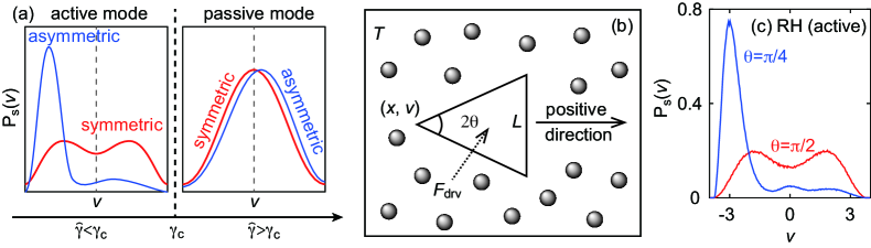
Figure 1: (a) Schematic of the active and the passive mode in one dimension. When $\hat{\gamma}<\gamma_{\textrm{c}}$ ($\hat{\gamma}>\gamma_{\textrm{c}}$) with a symmetric particle shape, the velocity distribution becomes symmetric bimodal (unimodal), which indicates the active (passive) mode as the left (right) red curve. When the shape of particle becomes asymmetric, one peak is amplified over the other for the active mode, while the peak position moves slightly aside for the passive mode (see the blue curves). (b) Schematic of the model. The t-particle is immersed in a reservoir with temperature $T$ and moves along the horizontal direction (one-dimensional motion). The reservoir consists of $N$ identical r-particles. The driving force, $F_{\textrm{drv}}$, is applied to the t-particle. (c) The steady-state velocity distributions for the RH model in the active mode. Red and blue curves are plots of numerical data for $\theta=\pi/2$ (symmetric) and $\pi/4$ (asymmetric), respectively. See SM Fig. S1 for numerical details and also for the distributions for the depot and the SG models.

In this Letter, we introduce the reverse situation where an asymmetric active particle is immersed in a reservoir of passive particles. This may describe the motion of a polar biological agent or motor inside a passive fluid such as water active_review . We find that the geometric asymmetry plays a crucial role for the rectified motion along with nonequilibrium-ness caused by the driving force in Eq. (4). We derive analytically the explicit formula for the rectified current and compare with numerical results via extensive molecular dynamics simulations. Surprisingly, a rectified current exists even in the passive mode, in particular for $\hat{\gamma}>0$ where the energy only dissipates (no energy pump-in). This is possible because thermal fluctuations are significantly reduced in this case, compensating the energy needed for generating an average current. This is why we coin the term “moving by dissipation” for this rectifying mechanism. In practice, this type of rectification provides a weak but reliable (less diffusive) directed motion even in highly fluctuating thermal environments.

Model – Consider a triangular shaped particle (t-particle) with mass $M$ and vertical cross section $L$ immersed in a reservoir with temperature $T$ as illustrated in Fig. 1(b). For simplicity, we constrain the t-particle motion along the horizontal direction only. Its apex angle, position, and velocity are denoted as $2\theta$, $x$, and $v$, respectively. The reservoir consists of $N$ identical circular shaped particles (r-particle) with mass $m$ and radius $R$ which move inside a two-dimensional square box with side length $l$ with periodic boundary conditions. We assume that $m\ll M$ and $R\ll L\ll l$.

The stochastic motion of the t-particle is induced by elastic collisions with r-particles, which are equipped with the Langevin thermostat. Details of collision dynamics and numerical simulations Broeck ; additivity are described in Supplementary Material (SM) I. Without any driving force, the t-particle reaches a thermal equilibrium with zero mean velocity. With a one-dimensional horizontal force in Eq. (4) applied on the t-particle, the system can be driven out of equilibrium. The red and blue curves in Fig. 1 (c) represent the numerical data for the steady-state velocity distributions of the t-particle with the symmetric shape $(\theta=\pi/2)$ and the asymmetric shape $(\theta=\pi/4)$ in the active mode for the RH model, respectively. Similar distributions for the depot and the SG models are presented in SM Fig. S1. Clear two symmetric red peaks denote the emergence of the nonzero self-propelled velocity with the zero average current for the symmetric case. In contrast, the shape asymmetry breaks the symmetry of the peaks, thus the active motion is rectified with a nonzero average current. Typical ‘run-and-tumble’ trajectories for the symmetric and asymmetric particle are shown in SM Fig. S2.

In the passive mode, we find a single peak at the zero velocity for the symmetric case, but at a small non-zero velocity for the asymmetric case, representing a weak rectified current, compared to that in the active mode. Figure 2 shows the $\hat{\gamma}$ dependence of the average current obtained from simulations and also from the analytic derivation in the small $m/M$ limit shown below.

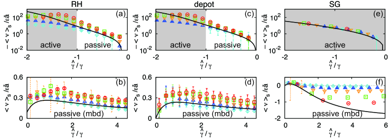
Figure 2: $\hat{\gamma}$ dependence of the rectified velocity for various self-propelling mechanisms. (a), (c), and (e) are the scaled steady-state velocities $\langle\nu\rangle_{\textrm{s}}/(\bar{a}\epsilon)$ as a function of $\hat{\gamma}/\gamma$ for the RH, the depot, and the SG models for negative $\hat{\gamma}$, respectively. (b), (d), and (f) are for positive $\hat{\gamma}$. Solid curves are analytic results for respective mechanisms. Cyan $\diamond$, blue $\vartriangle$, gold $\triangledown$, green $\square$, red $\circ$ points denote data for $M=5$, $10$, $20$, $50$, and $100$, respectively, with $m=1$ fixed. ‘mbd’ stands for ‘moving by dissipation’.

Perturbative analysis of the model – To understand the emergence of a nonzero current analytically, we present a perturbation theory for the t-particle dynamics for small $m/M$, which is reasonable in realistic situations. We also assume that r-particles are always in equilibrium. Then, our model can be described by the kinetic theory introduced in Ref. Broeck ; Meurs with the addition of an external driving force.

The probability density of the t-particle velocity $v$ at time $t$, $P(v,t)$, can be described by the following Boltzmann-Master equation:

$$\frac{\partial P(v,t)}{\partial t}=(\mathcal{L}_{\textrm{res}}+\mathcal{L}_{\textrm{drv}})P(v,t),$$ (5)

where $\mathcal{L}_{\textrm{res}}$ and $\mathcal{L}_{\textrm{drv}}$ are operators representing the effects of the reservoir and the driving force, respectively. More specifically, $\mathcal{L}_{\textrm{res}}$ can be written as

$$\mathcal{L}_{\textrm{res}}=\sum_{n=1}^{\infty}\frac{(-1)^{n}}{n!}\frac{\partial^{n}}{\partial v^{n}}a_{n}(v),$$ (6)

where a Kramers-Moyal coefficient $a_{n}(v)$ is defined as $a_{n}(v)\equiv\int r^{n}W(v+r|v)dr$ with the transition rate $W(v^{\prime}|v)$ from $v$ to $v^{\prime}$ induced by elastic collisions with r-particles Meurs ; Risken ; vanKampen . The explicit calculation of $a_{n}(v)$ is presented in SM II. $\mathcal{L}_{\textrm{drv}}$ is given by

$$\mathcal{L}_{\textrm{dis}}=-\frac{\partial}{\partial v}\frac{F_{\textrm{drv}}}{M},$$ (7)

with $F_{\textrm{drv}}=-\Gamma(v)v$ in Eq. (4).

It is convenient to introduce dimensionless variables

$$\nu\equiv v/v_{0}~{}~{}\left(v_{0}\equiv\sqrt{{k_{\textrm{B}}T}/{M}}\right)~{}~{}\textrm{ and }~{}~{}\tau=\gamma t/M,$$ (8)

where the t-particle friction coefficient $\gamma$ is obtained as

$$\gamma\equiv 4L\rho\sqrt{\frac{mk_{\textrm{B}}T}{2\pi}}(1+\sin\theta)~{},$$ (9)

with the r-particle density $\rho=N/l^{2}$ (see SM II). Then, Eq. (5) is rewritten as

$$\frac{\partial P(\nu,\tau)}{\partial\tau}=\sum_{n=1}^{\infty}\frac{(-1)^{n}}{n!}\frac{\partial^{n}}{\partial\nu^{n}}A_{n}(\nu)P(\nu,\tau),$$ (10)

where $A_{n}(\nu)$ is the modified Kramers-Moyal coefficient defined as

$$A_{n}(\nu)=\frac{M}{\gamma v_{0}^{n}}a_{n}(v_{0}\nu)-G(\nu)\nu\delta_{n,1}$$ (11)

with $P(\nu,\tau)=v_{0}P(v,t)$ and $G(\nu)=\Gamma(v_{0}\nu)/\gamma$.

We perform a perturbation expansion with the small parameter $\epsilon\equiv\sqrt{m/M}$. Up to ${\cal O}(\epsilon)$, we find in SM II

$$A_{1}(\nu) \approx-\left[1+G(\nu)\right]\nu+\bar{a}\left(1-\nu^{2}\right)\epsilon,$$

$$A_{2}(\nu) \approx 2+6\bar{a}\nu\epsilon,$$

$$A_{3}(\nu) \approx-12\bar{a}\epsilon,$$

$$A_{n}(\nu) ={\cal O}(\epsilon^{2}),~{}~{}\textrm{for}~{}n\geq 4,$$ (12)

where the asymmetric factor $\bar{a}=\frac{\sqrt{2\pi}}{4}(1-\sin\theta)\geq 0.$ Using Eqs. (10), (12) and the expansion of $P(\nu,\tau)\approx P^{(0)}(\nu,\tau)+\epsilon P^{(1)}(\nu,\tau)$, we can set up the equations as follows:

$$\partial_{\tau}P^{(0)}(\nu,\tau) =\mathcal{L}_{0}P^{(0)}(\nu,\tau)$$

$$\partial_{\tau}P^{(1)}(\nu,\tau) =\mathcal{L}_{1}P^{(0)}(\nu,\tau)+\mathcal{L}_{0}P^{(1)}(\nu,\tau)$$ (13)

where $\mathcal{L}_{0}$ and $\mathcal{L}_{1}$ are given by

$$\mathcal{L}_{0} =-\frac{\partial}{\partial\nu}\left[-\left(1+G(\nu)\right)\nu-\frac{\partial}{\partial\nu}\right]$$

$$\mathcal{L}_{1} =-\bar{a}\frac{\partial}{\partial\nu}\left[(1-\nu^{2})-3\frac{\partial}{\partial\nu}\nu-2\frac{\partial^{2}}{\partial\nu^{2}}\right].$$ (14)

The steady-state distribution of the zeroth order is then

$$P_{\textrm{s}}^{(0)}(\nu)=\frac{1}{\mathcal{N}}e^{-\int^{\nu}ds[1+G(s)]s}$$ (15)

with the normalization factor $\mathcal{N}$. The next order is obtained by solving $\mathcal{L}_{0}P_{\textrm{s}}^{(1)}(\nu)=-\mathcal{L}_{1}P_{\textrm{s}}^{(0)}(\nu)$. A straightforward analysis yields

$$P_{\textrm{s}}^{(1)}(\nu)=\bar{a}g(\nu)P_{\textrm{s}}^{(0)}(\nu)\quad\textrm{with}$$

$$g(\nu)=2G(\nu)\nu-\int_{0}^{\nu}ds~{}G(s)\left[1+2G(s)\right]s^{2}.$$ (16)

Note that $g(\nu)$ is an odd function of $\nu$, i.e., $g(-\nu)=-g(\nu)$, as $G(\nu)$ is even in $\nu$ in all models considered here. This is also consistent with the normalization condition $\int_{-\infty}^{\infty}dsP_{\textrm{s}}^{(1)}(s)=0$.

The steady-state average of the $n$-th moment of the velocity is then obtained up to ${\cal O}(\epsilon)$ as

$$\langle\nu^{n}\rangle_{\textrm{s}} \approx\int_{-\infty}^{\infty}d\nu~{}\nu^{n}\left[1+\bar{a}\epsilon g(\nu)\right]P_{\textrm{s}}^{(0)}(\nu)$$

$$=\left\{\begin{array}[]{ll}\bar{a}\epsilon\langle\nu^{n}g(\nu)\rangle_{0}&(n:\textrm{odd})\\ \langle\nu^{n}\rangle_{0}&(n:\textrm{even})\end{array}\right.,$$ (19)

where $\langle\cdots\rangle_{0}$ stands for the average over $P_{\textrm{s}}^{(0)}(\nu)$. Note that the average velocity as well as its all odd moments are ${\cal O}(\epsilon)$ and vanishes for the symmetric case ($\bar{a}=0$). Thus the time-reversal symmetry breaking (rectified current) occurs only with a shape asymmetry and a finite mass ratio. All even moments responsible for the stochasticity are always ${\cal O}(1)$, the same as that for $\bar{a}=0$. The standard fluctuation is simply given by the second moment; $\langle(\Delta\nu)^{2}\rangle_{s}=\langle\nu^{2}\rangle_{s}-\langle\nu\rangle_{s}^{2}\approx\langle\nu^{2}\rangle_{0}$ up to ${\cal O}(\epsilon)$. Similar results can be derived for the t-particle with an arbitrary convex shape.

Examples – We first consider a simple example with $F_{\textrm{drv}}=-\hat{\gamma}v$, yielding $G(\nu)=\hat{\gamma}/\gamma$. This model is known to describe a “cold damping” problem applicable to a molecular refrigerator Pinard ; Jourdan ; Kim . With Eqs. (15),  (16) and (19), we easily find the scaled rectified velocity and its fluctuation as

$$\langle\nu\rangle_{\textrm{s}}^{\textrm{sim}}=\bar{a}\varepsilon\frac{\hat{\gamma}/\gamma}{(1+\hat{\gamma}/\gamma)^{2}},\quad\langle\nu^{2}\rangle_{\textrm{s}}^{\textrm{sim}}=\frac{1}{1+\hat{\gamma}/\gamma}$$ (20)

with $P_{\textrm{s}}^{(0)}(\nu)\sim\exp[-(1+\hat{\gamma}/\gamma)\nu^{2}/2]$ (see SM III). As expected, the rectification is due to the interplay of nonequilibrium ($\hat{\gamma}$) and spatial asymmetry ($\bar{a}$), even though the driving force does not favor any particular spatial direction. In this simple model, only the passive mode ($\hat{\gamma}>-\gamma$) is allowed due to the dynamic instability in the active region. For $\hat{\gamma}>0$, we get a nonzero current without energy input by the driving force (rather dissipation only) - “moving by dissipation”. This can be understood that the driving force can generate the rectification energy by cooling down the t-particle (less fluctuation in Eq. (20)). Note that the t-particle can move in either direction, depending on the sign of $\hat{\gamma}$ and slows down for large positive $\hat{\gamma}$ until the motion is fully stalled at $\hat{\gamma}=\infty$.

Now, we consider the three models for active dynamics as in Eq. (4). We calculated the steady-state velocities $\langle\nu\rangle_{\textrm{s}}^{\textrm{RH}}$, $\langle\nu\rangle_{\textrm{s}}^{\textrm{dpt}}$, $\langle\nu\rangle_{\textrm{s}}^{\textrm{SG}}$, and their fluctuations for the RH, the depot, and the SG model, respectively. The calculation results are rather complicated, which are presented in SM III. The velocities are plotted as solid curves in Fig. 2, which show the stabilized active mode ($\hat{\gamma}/\gamma<-1$ for the RH and the depot model, and $\hat{\gamma}<0$ for the SG model) with a much bigger negative current, compared to that in the passive mode. In fact, $\langle\nu\rangle_{\textrm{s}}$ grows indefinitely as $\hat{\gamma}\rightarrow-\infty$ with huge energy pump-in by the driving force, and its fluctuation also diverges. In the passive mode, we find a weaker positive current for the RH and the depot model, similar to the above simple example for $\hat{\gamma}>0$. In contrast, the SG model shows an interesting crossover behavior from a positive to negative current for positive $\hat{\gamma}$ with $\langle\nu\rangle_{\textrm{s}}^{\textrm{SG}}=-2\bar{a}\epsilon$ in the $\hat{\gamma}\rightarrow\infty$ limit. This may be related to a faster decay of fluctuations in the SG model: $\langle\nu^{2}\rangle_{\textrm{s}}\sim\hat{\gamma}^{-2}$ (SG) and $\sim\hat{\gamma}^{-1}$ (RH and depot), see SM III and SM Fig. S7. Thus, the SG type would be more appropriate for designing reliable microscopic motors with both directional currents possible.

Numerical simulations – To confirm the validity of our analysis, we performed extensive molecular dynamics simulations explained in SM I. Data points in Fig. 2 are the simulation results for the rectified velocities of the asymmetric t-particle with various values of $\hat{\gamma}$ and t-particle mass $M=5,10,20,50,100$. All other parameters are fixed (see the caption of SM Fig. S1).

We find that their overall behaviors agree well with the theoretical predictions qualitatively, but with $\sim 40\%$ overestimates for the simple (SM Fig. S4), the RH, and the depot models in the small $\epsilon$ limit. The origin of this difference is unclear yet, but probably due to a reservoir finite-size effect, also noticed by previous studies in similar systems Broeck ; Meurs . For the SG model, the numerical over-estimate is much smaller, but the convergence to the small $\epsilon$ limit is quite slow for large positive $\hat{\gamma}/\gamma$. This slow convergence is also found in the active phase for the RH and the depot model. In order to understand the discrepancy between numerical and theoretical results systematically, further extensive simulations are necessary, which is out of scope of our research here.

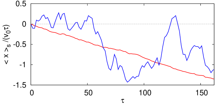
Figure 3: Trajectories of the t-particle averaged over 100 realizations driven by a constant force (blue) $f=5.1\times 10^{-3}\gamma v_{0}$ and the SG force with $\hat{\gamma}/\gamma=9.88$ (red).

The fluctuations are also plotted in SM Fig. S7. They agree very well with the theoretical predictions, except for the large-$\hat{\gamma}/\gamma$ region of the SG model, showing again a similar slow convergence. For highlighting the usefulness of the moving-by-dissipation mechanism, we compare two simulated trajectories of the same t-particle driven by either constant force ($F_{\textrm{drv}}=f$) or the SG force, resulting in the same average velocity. The blue (red) curve in Fig. 3 is the averaged trajectory over $100$ realizations when the t-particle is driven by the constant (SG) force. This clearly shows that the moving-by-dissipation mechanism can be utilized as a motor mechanism when an accurate motion is required in a highly fluctuating environment.

Conclusion – Our study clearly demonstrates that a self-propelled motion can be rectified by a geometric asymmetry of the active particle shape. We also show that this rectification is possible even in the passive mode. Especially, for $\hat{\gamma}>0$, the motion is driven by the moving-by-dissipation mechanism which can provide a novel design principle for developing more reliable microscopic motors. Our results are analytically derived by a relevant kinetic theory and supported qualitatively by numerical simulations. It is also imaginable that some microorganisms (and also nanomachines driven by chemical fuels) make use of this rectification mechanism by changing their shape asymmetrically to move in an intended direction.

- (1) P. Romanczuk, M. Bär, W. Ebeling, B. Lindner, and L. Schimansky-Geier, Active Brownian Particles. From Individual to Collective Stochastic Dynamics, Eur. Phys. J. Special Topics 202, 1–162 (2012).
- (2) X.-L. Wu and A. Libchaber, Particle Diffusion in a Quasi-Two-Dimensional Bacterial Bath, Phys. Rev. Lett. 84, 3017 (2000).
- (3) K. C. Leptos, J. S. Guasto, J. P. Gollub, A. I. Pesci, and R. E. Goldstein, Dynamics of Enhanced Tracer Diffusion in Suspensions of Swimming Eukaryotic Microorganisms, Phys. Rev. Lett. 103, 198103 (2009).
- (4) J. Palacci, C. Cottin-Bizonne, C. Ybert, and L. Bocquet, Sedimentation and Effective Temperature of Active Colloidal Suspensions, Phys. Rev. Lett. 105, 088304 (2010).
- (5) H. Kurtuldu, J. S. Guasto, K. A. Johnson, and J. P. Gollub, Enhancement of biomixing by swimming algal cells in two-dimensional films, Proc. Natl. Acad. Sci. USA 108, 10391 (2011).
- (6) C. Maggi, M. Paoluzzi, N. Pellicciotta, A. Lepore, L. Angelani, and R. Di Leonardo, Generalized Energy Equipartition in Harmonic Oscillators Driven by Active Baths, Phys. Rev. Lett. 113, 238303 (2014).
- (7) Y. Fily and M. C. Marchetti, Athermal Phase Separation of Self-Propelled Particles with No Alignment, Phys. Rev. Lett. 108, 235702 (2012).
- (8) S. Krishnamurthy, S. Ghosh, D. Chatterji, R. Ganapathy, and A. K. Sood, A micrometre-sized heat engine operating between bacterial reservoirs, Nature Phys. volume 12, 1134 (2016).
- (9) R. Zakine, A. Solon, T. Gingrich, and F. van Wijland, Stochastic Stirling Engine Operating in Contact with Active Baths, Entropy 19, 193 (2017).
- (10) J. S. Lee, J.-M. Park, and H. Park, Brownian heat engine with active reservoirs, Phys. Rev. E 102, 032116 (2020).
- (11) C. Kwon, J. Yeo, H. K. Lee, and H. Park, Unconventional entropy production in the presence of momentum-dependent forces, J. Korean Phys. Soc. 68, 633 (2016).
- (12) H. K. Lee, S. Lahiri, and H. Park, Nonequilibrium steady states in Langevin thermal systems, Phys. Rev. E 96, 022134 (2017).
- (13) É. Fodor, C. Nardini, M. E. Cates, J. Tailleur, P. Visco, and F. van Wijland, How Far from Equilibrium Is Active Matter?, Phys. Rev. Lett. 117, 038103 (2016).
- (14) L. Dabelow, S. Bo, and R. Eichhorn, Irreversibility in Active Matter Systems: Fluctuation Theorem and Mutual Information, Phys. Rev. X 9, 021009 (2019).
- (15) M. Badoual, F. Jülicher, and J. Prost, Bidirectional cooperative motion of molecular motors, Proc. Natl. Acad. Sci. USA 99, 6696-6701 (2002).
- (16) D. Chaudhuri, Active Brownian particles: Entropy production and fluctuation response, Phys. Rev. E 90, 022131 (2014).
- (17) C. Ganguly and D. Chaudhuri, Stochastic thermodynamics of active Brownian particles, Phys Rev E 88, 032102 (2013).
- (18) F. Schweitzer, W. Ebeling, and B. Tilch, Complex Motion of Brownian Particles with Energy Depots, Phys. Rev. Lett. 80, 5044 (1998).
- (19) W. Ebeling, F. Schweitzer, and B. Tilch, Active Brownian particles with energy depots modeling animal mobility, BioSystems 49, 17 (1999).
- (20) C. A. Condat, and G. J. Sibona, Diffusion in a model for active Brownian motion, Physica D: Nonlinear Phenomena 168, 235 (2002).
- (21) V. Garcia, M. Birbaumer, and F. Schweitzera, Testing an agent-based model of bacterial cell motility: How nutrient concentration affects speed distribution, Eur. Phys. J. B 82, 235-244 (2011).
- (22) M. Schienbein and H. Gruler, Langevin equation, Fokker-Planck equation and cell migration, Bull. Math. Biol. 55, 585 (1993).
- (23) U. Erdmann, W. Ebeling, L. Schimansky-Geier, F. Schweitzer, Brownian Particles far from Equilibrium, Eur. Phys. J. B 15, 105 (2000)
- (24) C. Van den Broeck, R. Kawai, and P. Meurs, Microscopic Analysis of a Thermal Brownian Motor, Phys. Rev. Lett. 93, 090601 (2004).
- (25) P. Meurs, C. Van den Broeck, and A. Garcia, Rectification of thermal fluctuations in ideal gases, Phys. Rev. E 70, 051109 (2004).
- (26) A. Sokolov, M. M. Apodaca, B. A. Grzybowski, and I. S. Aranson, Swimming bacteria power microscopic gears, Proc. Natl. Acad. Sci. USA 107, 969 (2010).
- (27) R. Di Leonardo, L. Angelani, D. Dell’Arciprete, G. Ruocco, V. Iebba, S. Schippa, M. P. Conte, F. Mecarini, F. De Angelis, and E. Di Fabrizio, Bacterial ratchet motors, Proc. Natl. Acad. Sci. USA 107, 9541 (2010).
- (28) L. Angelani, R. Di Leonardo, and G. Ruocco, Self-Starting Micromotors in a Bacterial Bath, Phys. Rev. Lett. 102, 048104 (2009).
- (29) Y. Baek, A. P. Solon, X. Xu, N. Nikola, and Y. Kafri, Generic Long-Range Interactions Between Passive Bodies in an Active Fluid, Phys. Rev. Lett. 120, 058002 (2018).
- (30) L. Angelani and R. Di Leonardo, Geometrically biased random walks in bacteria-driven micro-shuttles, New J. Phys. 12, 113017 (2010).
- (31) A. Kaiser, A. Peshkov, A. Sokolov, B. ten Hagen, H. Löwen, and I. S. Aranson, Transport Powered by Bacterial Turbulence, Phys. Rev. Lett. 112, 158101 (2014).
- (32) N. Nikola, A. P. Solon, Y. Kafri, M. Kardar, J. Tailleur, and R. Voituriez, Active Particles with Soft and Curved Walls: Equation of State, Ratchets, and Instabilities, Phys. Rev. Lett. 117, 098001 (2016).
- (33) C. J. O. Reichhardt and C. Reichhardt, Ratchet Effects in Active Matter Systems, Annu. Rev. Condens. Matter Phys. 8, 51 (2017).
- (34) J. S. Lee and H. Park, Additivity of multiple heat reservoirs in the Langevin equation, Phys. Rev. E 97, 062135 (2018).
- (35) H. Risken, The Fokker-Planck Equation (Springer, Berlin, 1989).
- (36) N. G. van Kampen, Stochastic Processes in Physics and Chemistry (Elsevier, 2007).
- (37) M. Pinard, P. F. Cohadon, T. Briant, and A. Heidmann, Full mechanical characterization of a cold damped mirror, Phys. Rev. A 63, 013808 (2000).
- (38) K. H. Kim and H. Qian, Entropy production of Brownian macromolecules with inertia, Phys. Rev. Lett. 93, 120602 (2004).
- (39) G. Jourdan, G. Torricelli, J. Chevrier, and F. Comin, Tuning the effective coupling of an AFM lever to a thermal bath, Nanotechnology 18, 475502 (2007).