Deep learning with transfer functions: new applications in system identification

Abstract

This paper presents a linear dynamical operator described in terms of a rational transfer function, endowed with a well-defined and efficient back-propagation behavior for automatic derivatives computation. The operator enables end-to-end training of structured networks containing linear transfer functions and other differentiable units by exploiting standard deep learning software. Two relevant applications of the operator in system identification are presented. The first one consists in the integration of prediction error methods in deep learning. The dynamical operator is included as the last layer of a neural network in order to obtain the optimal one-step-ahead prediction error. The second one considers identification of general block-oriented models from quantized data. These block-oriented models are constructed by combining linear dynamical operators with static nonlinearities described as standard feed-forward neural networks. A custom loss function corresponding to the log-likelihood of quantized output observations is defined. For gradient-based optimization, the derivatives of the log-likelihood are computed by applying the back-propagation algorithm through the whole network. Two system identification benchmarks are used to show the effectiveness of the proposed methodologies.

  To cite this work, please use the following bibtex entry:

@inproceedings{piga2021a,
  title={Deep learning with transfer functions:
            new applications in system identification},
  author={Piga, D. and Forgione, M. and Mejari, M.},
  booktitle={Proc. of the 19th IFAC Symposium System Identification:
                learning models for decision and control},
  address={Padova, Italy},
  year={2021}
}

Using the plain bibtex style, the bibliographic entry should look like:

D. Piga, M. Forgione and M. Mejari Deep learning with transfer functions: new applications in system identification. In Proc. of the 19th IFAC Symposium System Identification: learning models for decision and control, Padova, Italy, 2021.

 

1 Introduction

Thanks to the universal approximation capabilities of neural networks, deep learning algorithms are nowadays behind high-impact cutting-edge technologies such as language translation, speech recognition, and autonomous driving, just to cite a few [16]. Highly optimized and user-friendly deep learning frameworks are available [13], often distributed under permissive open-source licenses. On one hand, using the high-level functionalities offered by a deep learning framework, standard learning tasks (once considered extremely hard) such as image classification can be accomplished with moderate efforts even by non-expert practitioners. On the other hand, experienced users can build customized models and objective functions, exploiting the framework’s built-in back-propagation engine [15] for gradient computations.

System identification definitely represents a challenging field where the flexibility of neural networks and deep learning algorithms can be used to describe and estimate non-linear dynamical systems. This requires one to define specialized networks that take into account temporal evolution of the input/output data, a fundamental feature setting identification of dynamical systems apart from typical (static) supervised problems in machine learning.

Neural networks have been widely used in system identification in the past (see, e.g., [19, 3, 2]), and the back-propagation through time algorithm [20] has been applied to train Recurrent Neural Networks (RNNs). Recently, the use of Long Short-Term Memory (LSTM) and 1-D Convolutional Neural Networks (CNNs) in system identification has been discussed in [8, 18] and [1], respectively. An architecture specialized for continuous-time system identification called Integrated Neural Network, which consists of a feed-forward network followed by an integral block is proposed in [12]. Loss functions based on the simulation error over small subsets of the training data are proposed in [4, 5] and [14], where a regularization term and a multiple shooting approach are employed, respectively, to enforce that the initial conditions of all the subsets are compatible with the identified model dynamics. The list above is far from being exhaustive, as new contributions using neural networks and deep learning algorithms for system identification are regularly appearing every year in dedicated conferences and journals.

A novel network architecture called dynoNet which is tailored for the identification of nonlinear dynamical systems has been recently proposed by the authors in [6]. The network consists in the interconnection of Linear Time-Invariant (LTI) dynamical blocks and static nonlinearities. In this paper, we describe the LTI dynamical layer which constitutes the elementary block of dynoNet, along with the forward and backward operations needed to make this layer compatible with the back-propagation algorithm. The LTI layer is described in terms of rational transfer functions, and thus acts as an infinite impulse response (IIR) filter applied to its input sequence.

A differentiable LTI dynamical layer allows us to tackle several challenging problems in system identification. In particular, in this paper:

• We consider the case of output signals affected by an additive colored noise. To this aim, we include a trainable linear dynamical unit as the last layer of an end-to-end differentiable network representing a dynamical system (e.g., a convolutional, recurrent, or dynoNet network) in order to build the “one-step-ahead prediction error” minimized in the popular Prediction Error Method (PEM). Such an application of PEM in deep learning will be referred to as deepPEM;

• We address the problem of identification from quantized output observations, and present a method that is applicable to end-to-end differentiable model structures (including dynoNet), by properly changing the likelihood function maximized in training. As dynoNet represents a generalization of classic block-oriented architectures [7], the proposed approach can be applied for the identification of block-oriented models from quantized data.

The linear dynamical operator has been implemented in the PyTorch deep learning framework and the software is available for download at https://github.com/forgi86/sysid-transfer-functions-pytorch.

The rest of this paper is organized as follows. The linear dynamical operator is described in Section 2 and the steps required to integrate it in a deep learning framework are described in Section 3. The deepPEM algorithm and the problem of identification from quantized data are discussed in Section 4.1 and 4.2, respectively. Finally, two benchmark examples are presented in Section 5.

2 Dynamical layer

The input-output relation of the linear dynamical layer is described by a rational transfer function $G(q)$ as:

$$y(t)=G(q)u(t)=\frac{B(q)}{A(q)}u(t),$$ (1)

where $u(t)\in\mathbb{R}$ and $y(t)\in\mathbb{R}$ are the input and output signals of the filter $G(q)$ at time $t$ respectively, and $A(q)$ and $B(q)$ are polynomials in the time delay operator $q^{-1}$ ($q^{-1}u(t)=u(t-1)$), i.e.,

$$A(q) =1+a_{1}q^{-1}+\dots+a_{n_{a}}q^{-n_{a}},$$ (2a)

$$B(q) =b_{0}+b_{1}q^{-1}+\dots+b_{n_{b}}q^{-n_{b}}.$$ (2b)

The coefficients of the polynomials $A(q)$ and $B(q)$ are collected in vectors $a=[a_{1}\;a_{2}\dots\;a_{n_{a}}]\in\mathbb{R}^{n_{a}}$ and $b=[b_{0}\;b_{1}\;\dots\;b_{n_{b}}]\in\mathbb{R}^{n_{b}+1}$. They represent the tunable parameters of the filter $G(q)$.

The filtering operation in (1) has the following input/output representation:

$$A(q)y(t)=B(q)u(t),$$ (3)

which, according to the definitions of $A(q)$ and $B(q)$, is equivalent to the linear difference equation:

$$y(t)= -a_{1}y(t\!-\!1)\dots-a_{n_{a}}y(t\!-\!n_{a})+$$

$$+b_{0}u(t)+b_{1}u(t-1)+\dots+b_{n_{b}}\!u(t-n_{b}).$$ (4)

In the following, we assume that the filter $G(q)$ is always initialized from rest, i.e., $u(t)=0$ and $y(t)=0$ for $t<0$.

Let us stack the input and output samples $u(t)$ and $y(t)$ from time $0$ to $T\!-\!1$ in vectors $\mathbf{u}\in\mathbb{R}^{T}$ and $\mathbf{y}\in\mathbb{R}^{T}$, respectively. With a slight abuse of notation, the filtering operation in (1) applied to $\mathbf{u}$ is denoted as $\mathbf{y}=G(q)\mathbf{u}$. This operation is also equivalent to the convolution

$$\mathbf{y}_{i}=\sum_{j=\max{(0,i+1-T)}}^{\min(i,T-1)}\mathbf{g}_{j}\mathbf{u}_{i-j},\qquad i=0,1,\dots,T\!-\!1,$$ (5)

where $\mathbf{g}\in\mathbb{R}^{T}$ is a vector containing the first $T$ samples of the impulse response of $G(q)$.

The derivations are presented in the paper for a proper, single-input-single-output (SISO) transfer function to simplify the notation. Note that the software implementation available in the paper’s on-line repository allows setting an arbitraty number of input delays $n_{k}$, i.e. $B(q)=b_{0}q^{-n_{k}}+b_{1}q^{-n_{k}-1}+\dots+b_{n_{b}}q^{-(n_{k}-n_{b})}$ with $n_{k}\geq 0$, and includes support for the multi-input-multi-output (MIMO) case.

3 Dynamical Layer in Deep Learning

In this section, the forward and backward pass operations required to integrate the linear dynamical layer in a deep learning framework are derived. The operator $G(q)$ interpreted as a differentiable block for use in deep learning will be referred to as $G$-block in the rest of the paper.

3.1 Forward pass

The forward operations of a $G$-block are represented by solid arrows in the computational graph sketched in Fig. 1. In the forward pass, the block filters an input sequence $\mathbf{u}\in\mathbb{R}^{T}$ through a dynamical system $G(q)$ with parameters $a=[a_{1}\;\dots\;a_{n_{a}}]$ and $b=[b_{0}\;b_{1}\;\dots\;b_{n_{b}}]$. The block output $\mathbf{y}\in\mathbb{R}^{T}$ contains the filtered sequence:

$$\mathbf{y}=G(q,b,a)\mathbf{u}.$$ (6)

The input $\mathbf{u}$ of the $G$-block may be either the training input sequence or the result of previous operations in the computational graph, while the output $\mathbf{y}$ is an intermediate step towards the computation of a scalar loss $\mathcal{L}$.

Figure 1: Forward and backward operations of a $G$-block within a computational graph.

When the filtering operation (6) is implemented through the recurrent equation (2), the computational cost of the forward pass for the $G$-block corresponds to $T(n_{b}+n_{a}+1)$ multiplications. These multiplications need to be performed sequentially for the $T$ time samples, but can be parallelized for the $n_{b}$ + $n_{a}+1$ different coefficients at each time index $t$.

3.2 Backward pass

The backward operations are illustrated in Fig. 1 with dashed arrows. In the backward pass, the $G$-block receives the vector $\overline{\mathbf{y}}\in\mathbb{R}^{T}$ with the partial derivatives of the loss $\mathcal{L}$ w.r.t. $\mathbf{y}$, i.e.,

$$\overline{\mathbf{y}}_{t}=\frac{\partial\mathcal{L}}{\partial\mathbf{y}_{t}},\quad t=0,\dots,T-1,$$ (7)

and it has to compute the derivatives of the loss $\mathcal{L}$ w.r.t. its differentiable inputs $b$, $a$, and $\mathbf{u}$, i.e.,

$$\overline{b}_{j} =\frac{\partial\mathcal{L}}{\partial b_{j}},\qquad j=0,\dots,n_{b}$$ (8a)

$$\overline{a}_{j} =\frac{\partial\mathcal{L}}{\partial a_{j}},\qquad j=1,\dots,n_{a}$$ (8b)

$$\overline{\mathbf{u}}_{\tau} =\frac{\partial\mathcal{L}}{\partial\mathbf{u}_{\tau}},\qquad\tau=0,1,\dots,T\!-\!1.$$ (8c)

3.2.1 Derivatives w.r.t numerator coefficients $b$.

Application of the chain rule leads to:

$$\overline{b}_{j}=\sum_{t=0}^{T-1}\frac{\partial\mathcal{L}}{\partial\mathbf{y}_{t}}\frac{\partial\mathbf{y}_{t}}{\partial b_{j}}=\sum_{t=0}^{T-1}\overline{\mathbf{y}}_{t}\frac{\partial\mathbf{y}_{t}}{\partial b_{j}}$$ (9)

The sensitivities $\tilde{b}_{j}(t)=\frac{\partial\mathbf{y}_{t}}{\partial b_{j}}$, $j=0,1,\dots,n_{b},$ can be computed through recursive filtering operations [10]. Specifically, by differentiating the left hand side of Eq. (3) w.r.t $b_{j}$ we obtain:

$$A(q)\tilde{b}_{j}(t)=u(t-j),$$ (10)

Thus, $\tilde{b}_{j}(t)$ can be computed by filtering the input vector $u(t)$ through the linear filter $\displaystyle\frac{1}{A(q)}$. Furthermore,

$$\tilde{b}_{j}(t)=\begin{cases}\tilde{b}_{0}(t-j),\;\;&t-j\geq 0\\ 0,\;\;&t-j<0.\end{cases}$$ (11)

Then, only $\tilde{b}_{0}(t)$ needs to be recursively simulated through Eq. (10). The sensitivities $\tilde{b}_{j}(t)$, $j=1,\ldots,n_{b}$, are computed through simple shifting operations.

From (9) and (11), the $j$-th component of $\overline{b}$ is given by:

$$\overline{b}_{j}=\sum_{t=j}^{T-1}\overline{\mathbf{y}}_{t}\tilde{b}_{0}(t-j).$$ (12)

Overall, the computation of $\overline{b}$ requires to:

• filter the input $\mathbf{u}$ through $\frac{1}{A(q)}$, which entails $Tn_{a}$ multiplications. Because of the recursive form  of (10), these operations need to be performed sequentially;

• compute the $n_{b}\!+\!1$ dot products in (12), for a total of $T(n_{b}\!+\!1)-n_{b}$ multiplications. These operations can be parallelized.

3.2.2 Derivatives w.r.t denominator coefficients $a$.

The sensitivities $\tilde{a}_{j}(t)=\frac{\partial\mathbf{y}_{t}}{\partial a_{j}}$, $j=1,2,\dots,n_{a}$ are obtained based on the same rationale described above, by differentiating the terms in Eq. (3) with respect to $a_{j}$. This yields:

$$\tilde{a}_{j}(t)=-\frac{1}{A(q)}y(t-j).$$ (13)

The following condition holds:

$$\tilde{a}_{j}(t)=\begin{cases}\tilde{a}_{1}(t-j+1),\;\;&t-j+1\geq 0\\ 0,\;\;&t-j+1<0\end{cases}$$ (14)

and the $j$-th component of $\overline{a}$ is given by:

$$\overline{a}_{j}=\sum_{t=j-1}^{T-1}\overline{\mathbf{y}}_{t}\tilde{a}_{1}(t-j+1).$$ (15)

The back-propagation for the coefficients $a$ thus requires: ($i$) the filtering operation (13), which involves $Tn_{a}$ multiplications; and ($ii$) the $n_{a}$ dot products defined in (15), for a total of $Tn_{a}-n_{a}+1$ multiplications.

3.2.3 Derivatives w.r.t. input time series $\mathbf{u}$.

In order to compute the partial derivatives $\frac{\partial\mathcal{L}}{\partial\mathbf{u}_{\tau}}$ the chain rule is applied, which yields:

$$\overline{\mathbf{u}}_{\tau}=\frac{\partial\mathcal{L}}{\partial\mathbf{u}_{\tau}}=\sum_{t=0}^{T-1}{\frac{\partial\mathcal{L}}{\partial\mathbf{y}_{t}}\frac{\partial\mathbf{y}_{t}}{\partial\mathbf{u}_{\tau}}}=\sum_{t=0}^{T-1}{\overline{\mathbf{y}}_{t}\frac{\partial\mathbf{y}_{t}}{\partial\mathbf{u}_{\tau}}}$$ (16)

From (5), the term $\frac{\partial\mathbf{y}_{t}}{\partial\mathbf{u}_{\tau}}$ is given by:

$$\frac{\partial\mathbf{y}_{t}}{\partial\mathbf{u}_{\tau}}=\begin{cases}\mathbf{g}_{t-\tau},\;\;&t-\tau\geq 0\\ 0,\;&t-\tau<0.\end{cases}$$ (17)

By substituting Eq. (17) into (16), we obtain

$$\overline{\mathbf{u}}_{\tau}=\sum_{t=\tau}^{T-1}\overline{\mathbf{y}}_{t}\mathbf{g}_{t-\tau}$$ (18)

Direct implementation of the cross-correlation (18) requires a number of operations which grows quadratically with $T$. A more efficient solution is obtained by observing:

$$\overline{\mathbf{u}}_{0}=\sum_{t=0}^{T-1}\overline{\mathbf{y}}_{t}\mathbf{g}_{t},\ \ \ \ \overline{\mathbf{u}}_{1}=\sum_{t=1}^{T-1}\overline{\mathbf{y}}_{t}\mathbf{g}_{t-1},\ \ \ \ \overline{\mathbf{u}}_{2}=\sum_{t=2}^{T-1}\overline{\mathbf{y}}_{t}\mathbf{g}_{t-2},$$

$$\dots,\ \ \ \ \overline{\mathbf{u}}_{T-2}=\overline{\mathbf{y}}_{T-2}\mathbf{g}_{0}+\overline{\mathbf{y}}_{T-1}\mathbf{g}_{1},\ \ \ \ \ \overline{\mathbf{u}}_{T-1}=\overline{\mathbf{y}}_{T-1}\mathbf{g}_{0}.$$

Since $\mathbf{g}$ represents the impulse response of $G(q)$, the vector $\overline{\mathbf{u}}$ can be obtained by filtering the vector $\overline{\mathbf{y}}$ in reverse time through $G(q)$, and then reversing the result, i.e.,

$${\overline{\mathbf{u}}}=\textrm{flip}\big{(}G(q)\textrm{flip}(\overline{\mathbf{y}})\big{)},$$ (19)

where $\textrm{flip}(\cdot)$ denotes the time reversal operator applied to a $T$-length vector, defined as

$$\left(\textrm{flip}(\mathbf{x})\right)_{t}=\mathbf{x}_{T-t-1},\qquad t=0,1,\dots,T-1.$$ (20)

Eq. (19) represents the filtering of a $T$-length vector through $G(q)$, whose complexity grows linearly with $T$.

4 Applications in system identification

4.1 deepPEM

As a first application of the differentiable LTI layer discussed in the previous section, we integrate PEM in a deep learning context. To this aim, let us consider the data-generating system which provides the output $y$ at time $t$ according to the equation:

$$y(t)=\mathcal{S}(U_{t})+\overbrace{H_{\rm o}(q)e(t)}^{=v(t)},$$ (21)

where $\mathcal{S}(\cdot)$ is the deterministic causal component processing the entire past input sequence $U_{t}$ up to time $t$, and $v(t)$ is an additive colored noise source obtained by filtering a white noise $e(t)$ through a stable linear filter $H_{\rm o}$. According to the PEM framework [10, Ch. 2.3], we assume that $H_{\rm o}$ is monic and minimum phase.

Let us now consider a model structure

$$y(t)=\mathcal{M}(U_{t},\theta_{\mathcal{M}})+H(q,\theta_{H})e(t),$$ (22)

where $\mathcal{M}(U_{t},\theta_{\mathcal{M}})$ is a deterministic causal component (described by the parameter vector $\theta_{\mathcal{M}}$) modeling the deterministic component $\mathcal{S}(U_{t})$ in (21) and $H(q,\theta_{H})$ is a transfer function with parameters $\theta_{H}=[a_{H}\ b_{H}]$. We denote with $\theta=[\theta_{\mathcal{M}}\ \theta_{H}]$ the vector containing all the unknown parameters in (22).

As known (see  [10, Ch. 2.3]), the optimal one-step-ahead predictor for (22) at time $t$, given input and output data up to time $t-1$, is given by

$$\hat{y}(t|t-1)=H^{-1}(q,\theta_{H})\mathcal{M}(U_{t},\theta_{\mathcal{M}})\\ +[1\!-\!H^{-1}(q,\theta_{H})]y(t).$$ (23)

Note that the output predictor in (23) only depends on outputs up to time $t-1$ since $\!H^{-1}(q,\theta_{H})$ is monic. The prediction error $\varepsilon(t)=y(t)-\hat{y}(t|t-1)$ is then given by

$$\varepsilon(t,\theta)=H^{-1}(q,\theta_{H})(y(t)-\mathcal{M}(U_{t},\theta_{\mathcal{M}})).$$ (24)

According to the Prediction Error Minimization (PEM) criterion, we consider the loss function:

$$\mathcal{L}(\theta)=\frac{1}{T}\sum_{t=0}^{T-1}\ell(\bm{\varepsilon}_{t}(\theta)),$$ (25)

where $\bm{\varepsilon}\in\mathbb{R}^{T}$ is the vector stacking the prediction error $\varepsilon$ from time $0$ up to $T-1$, and $\ell(\cdot)$ is a scalar-valued function (e.g., $\ell(\bm{\varepsilon}_{t}(\theta))=\bm{\varepsilon}^{2}_{t}(\theta)$).

The differentiable transfer function discussed in this paper enables easy implementation of the PEM framework for models where the deterministic component $\mathcal{M}(\cdot,\theta_{\mathcal{M}})$ is compatible with back-propagation. For instance, $\mathcal{M}(\cdot,\theta_{\mathcal{M}})$ could be a RNN, a 1-D CNN, or a dynoNet.

The corresponding computational graph for deepPEM is outlined in Fig. 2. Note that the monic transfer function $H^{-1}(q,\theta)$ is constructed as

$$H^{-1}(q,\theta_{H})=1+\check{H}(q,\theta_{H}),$$

where $\check{H}(q,\theta_{H})$ is a strictly proper transfer function implemented as a $G$-block with one input delay ($n_{k}\!=\!1$). This makes the estimated $H^{-1}(q,\theta_{H})$ monic by construction.

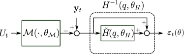
Figure 2: deepPEM: block diagram representing the computation of the one-step-ahead prediction error.

4.2 Learning from quantized observations

As a second application, we consider the problem of learning dynamical systems from quantized output measurements. Specifically, we assume that at each time $t$ we observe a quantized output $\mathbf{z}_{t}\in\{0,1,\ldots,K\!-\!1\}$. The integer $K$ represents the number of quantization intervals and $\mathbf{z}_{t}$ is given by

$$\mathbf{z}_{t} =Q(\mathbf{y}_{t}+\mathbf{e}_{t}),$$ (26a)

where $\mathbf{y}_{t}$ is the latent non-quantized output of the underlying data generating system, $\mathbf{e}_{t}$ is a zero-mean white Gaussian noise with (unknown) standard deviation $\sigma_{e}$, and $Q(\cdot)$ is the quantizing operator, defined as

$$Q(x)=m\;\;\text{if}\;\;x\in(q_{m},q_{m+1}],$$ (27)

with $(q_{m},q_{m+1}]$ denoting the $m$-th quantization interval.

Let us consider a simulation model $\mathcal{M}(\cdot,\theta_{\mathcal{M}})$ parametrized by a vector $\theta_{\mathcal{M}}$ which provides an output $\mathbf{y}^{{\rm sim}}_{t}$ when fed with an input sequence $U_{t}$, i.e., $\mathbf{y}^{{\rm sim}}_{t}=\mathcal{M}(U_{t},\theta_{\mathcal{M}})$.

Because of the conditional independence of the observed outputs $\mathbf{z}_{t}$ given the non-quantized output $\mathbf{y}_{t}$, the log-likelihood function of the parameters $\theta=[\theta_{\mathcal{M}}\ \sigma_{e}]$ is:

$$\mathcal{L}(\theta)= \sum_{t=0}^{T-1}\log\left[p(Q(\mathbf{y}^{{\rm sim}}_{t}+\mathbf{e}_{t})=\mathbf{z}_{t})\right]$$

$$= \sum_{t=0}^{T-1}\log\left[p(q_{\mathbf{z}_{t}}<\mathbf{y}^{{\rm sim}}_{t}+\mathbf{e}_{t}\leq q_{\mathbf{z}_{t+1}})\right]$$

$$= \sum_{t=0}^{T-1}\underset{\mathcal{L}_{t}(\theta)}{\underbrace{\log\left[\Phi\left(\frac{q_{\mathbf{z}_{t+1}}-\mathbf{y}^{{\rm sim}}_{t}}{\sigma_{e}}\right)\!-\!\Phi\left(\frac{q_{\mathbf{z}_{t}}\!-\!\mathbf{y}^{{\rm sim}}_{t}}{\sigma_{e}}\right)\right]}},$$ (28)

where $\Phi$ is the cumulative density function of the Normal distribution, i.e., $\Phi(x)=\int_{w=-\infty}^{x}\mathcal{N}(w;0,1)dw$.

The log-likelihood (4.2) may be readily implemented in current deep learning software frameworks using standard differentiable blocks. The block diagram corresponding to the log-likelihood $\mathcal{L}_{t}(\theta)$ of a single quantized observation $\mathbf{z}_{t}$ is sketched in Fig. 3. The model $\mathcal{M}(\cdot,\theta_{\mathcal{M}})$ can be a dynoNet network, which allows us to train block-oriented models (constituted by trainable $G$-blocks followed by static nonlinearities) from quantized output observations.

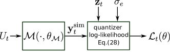
Figure 3: Learning from quantized data: block diagram representing the computation of the log-likelihood $\mathcal{L}_{t}(\theta)$ (4.2) of the quantized output sample $\mathbf{z}_{t}$.

5 Examples

The effectiveness of the proposed methodologies is evaluated on benchmark datasets for system identification available at the website www.nonlinearbenchmark.org. We present, in particular, results based on the Wiener-Hammerstein (WH) and the parallel Wiener-Hammerstein (PWH) benchmarks described in [11] and [17], respectively. The original training datasets of the two benchmarks are modified to make the identification problem more challenging and to highlight flexibility of the presented methodologies in handling non-standard learning problems. For the WH benchmark, we perturb the output with an additive colored noise and adopt the deepPEM method described in Section 4.1 to estimate the WH model parameters and the power spectrum of the noise. For the PWH benchmark, we consider the case of quantized output measurements and estimate the model parameter by maximizing the log-likelihood (4.2).

We use dynoNet networks to describe the deterministic system component in the two benchmarks, with an obvious choice of the network architectures reflecting the block-oriented structures of the PWH and WH systems.

All computations are carried out on a PC equipped with an AMD Ryzen 5 1600x processor and 32 GB of RAM. The codes required to reproduce the results are available in the GitHub repository https://github.com/forgi86/sysid-transfer-functions-pytorch.git. The reader is referred to [6] for further examples showing the effectiveness of dynoNet.

5.1 Training settings and metrics

The Adam algorithm [9] is used for gradient-based optimization. The number $n$ of iterations is chosen sufficiently large to reach a cost function plateau. The learning rate $\lambda$ is adjusted by a rough trial and error. All static non-linearities are modeled as feed-forward Neural Networks with a single hidden layer containing 10 neurons and hyperbolic tangent activation function.

The $\mathrm{fit}$ index and the Root Mean Square Error (RMSE) are used to assess the quality of the identified models:

$$\mathrm{fit} =100\cdot\left(1-\frac{\sqrt{\sum_{t=0}^{T-1}\left(\mathbf{y}_{t}-\mathbf{y}^{{\rm sim}}_{t}\right)^{2}}}{\sqrt{\sum_{t=0}^{T-1}\left(\mathbf{y}_{t}-{\overline{{\mathbf{y}}}}\right)^{2}}}\right)(\%),$$

$$\mathrm{RMSE} =\sqrt{\frac{1}{T}\sum_{t=0}^{T-1}\left(\mathbf{y}_{t}-\mathbf{y}^{{\rm sim}}_{t}\right)^{2}},$$

where $\mathbf{y}^{{\rm sim}}_{t}$ is the open-loop simulated output of the estimated model and $\overline{\mathbf{y}}$ is the average of the measured output sequence. Both the $\mathrm{fit}$ and the RMSE indexes are measured on the benchmarks’ original test data.

5.2 WH with colored noise

The experimental setup used in this benchmark is an electronic circuit described in [11] that behaves as a Wiener-Hammerstein system. Therefore, a simple dynoNet architecture corresponding to the WH model structure is adopted. Specifically, the dynoNet model used has a sequential structure defined by a SISO $G$-block with $n_{a}=n_{b}=8,n_{k}=1$; a SISO feed-forward neural network; and a final SISO $G$-block with $n_{a}=n_{b}=8,n_{k}=0$.

The original training dataset is modified by adding to the measured output a colored noise $v$ with standard deviation $0.1$ obtained by filtering a white noise $e$ through the transfer function $H_{\rm o}(q)=\frac{1-1.568q^{-1}+0.902q^{-2}}{1-1.901q^{-1}+0.9409q^{-2}}$.

In order to jointly estimate the system and the noise disturbance, the deepPEM approach presented in Section 4.1 is applied. The model is trained over $n=40000$ iterations of the Adam algorithm with learning rate $\lambda=10^{-4}$ on the whole training dataset ($T=100000$ samples). The total training time is 267 seconds.

On the test dataset ($T=87000$ samples), the performance of the identified dynoNet model are $\rm fit\!=\!96.9\%$ and $\rm{RMSE}\!=\!7.5$ mV. The measured output $\mathbf{y}$ and simulated output $\mathbf{y}^{{\rm sim}}$ on the test dataset are shown in Fig 4, together with the simulation error $\mathbf{e}=\mathbf{y}\!-\!\hat{\mathbf{y}}$. The magnitude Bode plot of the noise filter $H_{\rm o}(q)$ and of the identified $H(q,\theta_{H})$ are reported in Fig. 5. The obtained results show the capabilities of the deepPEM in accurately reconstructing the system’s output and the noise spectrum.

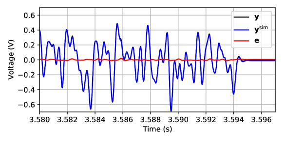
Figure 4: WH benchmark: measured output $\mathbf{y}$ (black), simulated output $\mathbf{y}^{{\rm sim}}$ (blue), and simulation error $\mathbf{e}\!=\!\mathbf{y}\!-\!\mathbf{y}^{{\rm sim}}$ (red) on the test dataset.

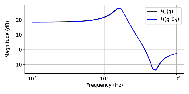
Figure 5: WH benchmark: Magnitude Bode plot of the filter $H_{\rm o}(q)$ and of the estimated filter $H(q,\theta_{H})$.

5.3 PWH with quantized observations

The experimental setup used in the second benchmark is an electronic circuit with a two-branch parallel Wiener-Hammerstein structure described in [17]. The original training dataset of the PWH benchmark consists in 100 input/output training sequences, each one containing $N=16384$ samples. The 100 training sequences are obtained by exciting the system with random-phase multisine input signals at 5 different rms levels: $\{100,325,550,775,1000\}$ mV, for 20 different realizations of the random phases. In this paper, we modify the original training dataset by discretizing the measured output voltage in $12$ equally spaced bins in the range $[-1\ \ 1]~{}V$. It is worth pointing out that in the benchmark datasets associated to rms levels equal to $100$ mV and $325$ mV, the chosen quantization intervals lead to quantized outputs that only take $2$ different values.

As a simulation model $\mathcal{M}(\cdot,\theta_{\mathcal{M}})$ (see Fig. 3) we use a sequential dynoNet network corresponding to the PWH structure and constructed as the cascade connection of: a one-input-two-output $G$-block; two independent one-input-one-output feed-forward neural networks; and a two-input-one-output $G$-blocks. The $G$-blocks are characterized by $n_{a}=12$, $n_{b}=12$, and $n_{k}=1$.

We train the dynoNet network by maximizing the log-likelihood $\mathcal{L}(\theta)$ (Eq. (4.2)) on the whole training dataset over $n=4000$ iterations with learning rate $\lambda=10^{-3}$. In the benchmark, 6 test datasets are provided. In the first 5 test datasets, the input signals are random-phase multisine at the same rms levels considered in training (but with independent phase realizations), while in the latter the input signal is filtered Gaussian noise with an envelope that grows linearly over time. On the 6 test datasets, the model achieves $\rm fit$ index $\{91.1,93.5,94.1,94.1,93.3,91.9\}\%$ and RMSE $\{3.65,8.20,12.02,16.04,22.06,21.37\}$ mV. Time traces of the measured and simulated dynoNet output on the growing envelope test dataset are shown in Fig. 6.

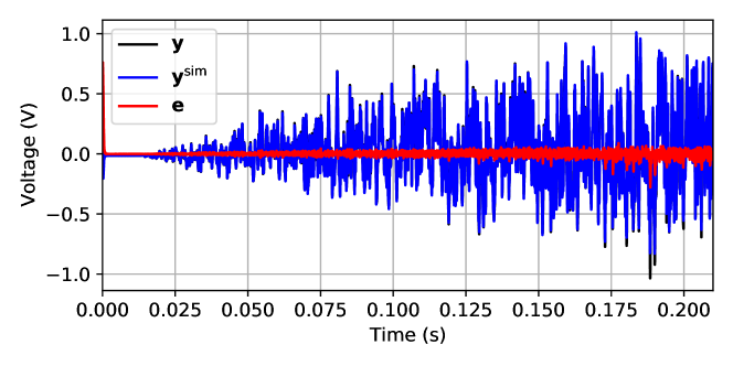
Figure 6: PWH benchmark: measured output $\mathbf{y}$ (black), simulated output $\mathbf{y}^{{\rm sim}}$ (blue), and simulation error $\mathbf{e}\!=\!\mathbf{y}\!-\!\mathbf{y}^{{\rm sim}}$ (red) on the growing envelope test dataset.

6 Conclusions

We have described the operations required to make the linear time-invariant transfer functions fully compatible with the back-propagation algorithm. This enables training of structured models combining transfer functions with other differentiable operators (such as deep neural networks) using standard deep learning software. Furthermore, dynoNet allows us to train dynamical models without using back-propagation through time.

Furthermore, we have illustrated two applications of the back-propagation-compatible linear dynamical block in system identification, namely the extension of the prediction error method to non-linear neural models in the presence of additive colored noise and the estimation of block-oriented models from quantized output observations.

Current research is devoted to the analysis of neural model structures containing transfer functions through linear system theory, to applications of these networks in other domains such as state estimation and time series classification, and to the extension of the $G$-block to the case of linear dynamics with parameter-varying coefficients.

References

- [1] C. Andersson, A. H. Ribeiro, K. Tiels, N. Wahlström, and T. B. Schön. Deep convolutional networks in system identification. IEEE 58th Conference on Decision and Control, pages 3670–3676, Nice, France, 2019.
- [2] SABS Chen and SA Billings. Neural networks for nonlinear dynamic system modelling and identification. International journal of control, 56(2):319–346, 1992.
- [3] Sheng Chen, SA Billings, and PM Grant. Non-linear system identification using neural networks. International Journal of Control, 51(6):1191–1214, 1990.
- [4] Marco Forgione and Dario Piga. Model structures and fitting criteria for system identification with neural networks. In Proc. of the 14th IEEE International Conference Application of Information and Communication Technologies, Tashkent, Uzbekistan, 2020.
- [5] Marco Forgione and Dario Piga. Continuous-time system identification with neural networks: model structures and fitting criteria. European Journal of Control, 59:69–81, 2021.
- [6] Marco Forgione and Dario Piga. dynoNet: A neural network architecture for learning dynamical systems. International Journal of Adaptive Control and Signal Processing, 35(4), 2021.
- [7] F. Giri and E. Bai. Block-oriented Nonlinear System Identification, volume 404 of Lecture Notes in Control and Information Sciences. Springer, 2010.
- [8] Jesús Gonzalez and Wen Yu. Non-linear system modeling using LSTM neural networks. IFAC-PapersOnLine, 51(13):485–489, 2018.
- [9] D.P. Kingma and J. Ba. Adam: A method for stochastic optimization. 3rd International Conference on Learning Representations, San Diego, CA, USA, 2015.
- [10] L. Ljung. System Identification: Theory for the User. Prentice Hall PTR, Upper Saddle River, NJ, USA, 1999.
- [11] L. Ljung, J. Schoukens, and J. Suykens. Wiener-Hammerstein benchmark. 15th IFAC Symposium on System Identification, Saint-Malo, France, 2009.
- [12] B. Mavkov, M. Forgione, and D. Piga. Integrated neural networks for nonlinear continuous-time system identification. IEEE Control Systems Letters, 4(4):851–856, 2020.
- [13] A. Paszke, S. Gross, S. Chintala, G. Chanan, E. Yang, Z. DeVito, Z. Lin, A. Desmaison, L. Antiga, and A. Lerer. Automatic differentiation in PyTorch. NIPS Autodiff Workshop, Long Beach, California, 2017.
- [14] Antônio H. Ribeiro, Koen Tiels, Jack Umenberger, Thomas B. Schön, and Luis A. Aguirre. On the smoothness of nonlinear systemidentification. Automatica, 121, 2020.
- [15] David E Rumelhart, Geoffrey E Hinton, Ronald J Williams, et al. Learning representations by back-propagating errors. Cognitive modeling, 5(3), 1988.
- [16] Jürgen Schmidhuber. Deep learning in neural networks: An overview. Neural networks, 61:85–117, 2015.
- [17] Maarten Schoukens, Anna Marconato, Rik Pintelon, Gerd Vandersteen, and Yves Rolain. Parametric identification of parallel Wiener–Hammerstein systems. Automatica, 51:111–122, 2015.
- [18] Yu Wang. A new concept using LSTM neural networks for dynamic system identification. In 2017 American Control Conference (ACC), pages 5324–5329, 2017.
- [19] Paul J Werbos. Neural networks for control and system identification. In 28th IEEE Conference on Decision and Control, pages 260–265, 1989.
- [20] Ronald J Williams and David Zipser. Oxford Handbook of Innovation. Erlbaum Associates, Hillsdale, NJ, USA, 1995.