WiFiMod: Transformer-based Indoor Human Mobility Modeling using Passive Sensing

Abstract.

Modeling human mobility has a wide range of applications from urban planning to simulations of disease spread. It is well known that humans spend  80% of their time indoors but modeling indoor human mobility is challenging due to three main reasons: (i) the absence of easily acquirable, reliable, low-cost indoor mobility datasets, (ii) high prediction space in modeling the frequent indoor mobility, and (iii) multi-scalar periodicity and correlations in mobility. To deal with all these challenges, we propose WiFiMod, a Transformer-based, data-driven approach that models indoor human mobility at multiple spatial scales using WiFi system logs. WiFiMod takes as input enterprise WiFi system logs to extract human mobility trajectories from smartphone digital traces. Next, for each extracted trajectory, we identify the mobility features at multiple spatial scales, macro and micro, to design a multi-modal embedding Transformer that predicts user mobility for several hours to an entire day across multiple spatial granularities. Multi-modal embedding captures the mobility periodicity and correlations across various scales while Transformers capture long term mobility dependencies boosting model prediction performance. This approach significantly reduces the prediction space by first predicting macro mobility, then modeling indoor scale mobility, micro mobility, conditioned on the estimated macro mobility distribution, thereby using the topological constraint of the macro-scale. Experimental results show that WiFiMod achieves a prediction accuracy of at least 10% points higher than the current state-of-art models. Additionally, we present 3 real-world applications of WiFiMod - (i) predict high density hot pockets and space utilization for policy making decisions for COVID19 or ILI, (ii) generate a realistic simulation of indoor mobility data to simulate spread of diseases, (iii) design personal assistants.

1. Introduction

Understanding human mobility is fundamental to location based services, urban transportation, and smart cities among many other applications and paramount to improve sustainability. Lately, with the advances in networking technologies and ubiquity of mobile phones, a large amount of mobility data is generated and collected in the form of GPS logs, cellular data, social media check-ins, and vehicular data giving rise to data-driven human mobility modeling (Hang et al., 2018; Veloso et al., 2011; Hasan et al., 2013; Jurdak et al., 2015). This prior work seeks to capture human mobility at urban scales (Isaacman et al., 2012) using transportation, social media, and phone data. While taxi or public transit data (Ganti et al., 2013; Veloso et al., 2011) allow urban-scale mobility of users to be captured from a vehicular or transportation standpoint, social media check-in data (Jurdak et al., 2015) enables users’ mobility to be tracked at various points of interest (Hasan et al., 2013). GPS and cellular data from phones have also been used to capture urban mobility patterns, with GPS capturing fine outdoor mobility and cellular data capturing coarse mobility (Huang et al., 2010). However, all these modeling efforts focus on outdoor or macro scale human mobility across various Point of Interest (POI), locations, or city regions.

Studies have shown that humans spend over 80% of their lives indoors (Arif et al., 2016) resulting in indoor or micro mobility. Recent research has recognized that indoor mobility of users inside buildings, where many users spend a significant portion of the day, is very different from outdoor mobility exhibited when walking in a city or traveling in vehicles (Zheng et al., 2018; Zhou et al., 2017). As we model mobility at a finer spatial scale, mobility becomes more frequent and the prediction space expands. We argue that the motivation for indoor mobility, as well as the region of movement, is time-dependent and micro mobility shows high correlations to the macro mobility features of context, location type, and location name. Moreover, indoor mobility displays a complex sequential periodicity correlated to the macro, outdoor or coarse grained, features of mobility. Due to the above stated reasons, we cannot directly use outdoor mobility models that capture mobility at large grid or POI levels at a single spatial scale for indoor mobility modeling.

In this work, we present WiFiMod, a transformer-based multi-scale indoor mobility model that uses existing WiFi infrastructure to passively sense human mobility. In pursuit of this model, we have three specific goals. First, we argue that human mobility is inherently hierarchical, where macro mobility, user type, and time of the day determine the micro mobility. Second, we capture the multi-modal features of macro as well as micro mobility patterns by creating a joint embedding and learn the correlations to generate sequences of context (Work or Home), building type (describes the space usage), building name (unique building identifier), and indoor location (room number, floor, or zone). The multi-modal embedding captures how individuals move between indoor spaces across and within buildings and takes into account how different space types exhibit distinct mobility patterns over time due to differences in space utilization. Third, we provide a ready-to-deploy system that uses existing ubiquitous WiFi infrastructure present at all enterprise networks and uses system log (syslog) messages to extract indoor human mobility.

Our main contributions in this work can be summarized as follows:

• We design an end-to-end data-driven approach to model indoor human mobility using passive WiFi sensing. WiFi logs based passive sensing approach uses already existing WiFi infrastructure in an enterprise or campus network providing a reliable indoor mobility dataset.

• We propose the use of multi-modal embedding to capture the macro and micro mobility features along with their correlations to improve the model prediction accuracy.

• We demonstrate the efficacy of our model by evaluating it against a real world dataset of 2500 users in a large campus setting and show that our model shows superior performance by at least 10% points over other indoor mobility models.

• We present three case studies that demonstrate the use of our model in predicting indoor hot pockets or high human density zones, generating user mobility trajectories, and designing personal assistants.

2. Background and User Data Ethics

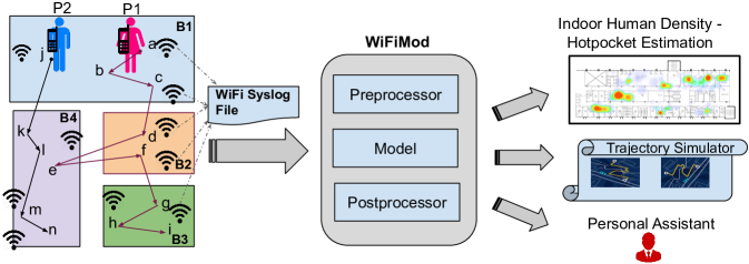
Figure 1. WiFiMoD : An indoor mobility modeling approach using WiFi sensing.

In this section, we present the background for our work on data-driven indoor mobility modeling.

Mobility as Nomadic Behavior: Some mobility models, such as the classic random waypoint model, emphasize modeling the physical movement of users such as velocity, acceleration, and direction of movement (Camp et al., 2002; Davies et al., 2000). In contrast, several other models, including our work, view user mobility as inherently nomadic. Nomadic user mobility can be seen as a sequence of location visits, where users visit a location to spend some time at that location known as a dwell period then transition to another location, followed by a dwell period at the new location and so on (Qiao et al., 2018). Figure  1 shows two users P1 and P2 visiting multiple buildings B1 through B4 and spending time at various locations. Each dwell period at buildings B1 through B4 for P1 and P2 is followed by a transition. In this case, the emphasis is on which locations are visited at various times of the day, across multiple buildings, building types, and context, revealing the semantic meaning of the nomadic behavior. Since humans are creatures of habits and tend to follow a routine (Song et al., 2010), we need to capture the correlations such as repeating visits to a location, repeating sequences resulting from daily or weekly routines, long-term dependencies, and affinity to certain locations, to name a few. While transitions from one location to another also need to be modeled, the emphasis is on capturing nomadic behavior, rather than factors such as the speed of mobility, the direction of movement, mode of transport, etc. Since, our primary focus is on modeling indoor mobility, modeling nomadic behavior is more appropriate since users are often stationary inside the building - in their office, in meetings, etc.

Modeling Trajectories: Mobility models come in many different flavors depending on what aspects of mobility the model is attempting to capture. A common type of mobility modeling to capture nomadic behavior is next location prediction (Do and Gatica-Perez, 2012; Liu et al., 2016; Lin et al., 2012; Gambs et al., 2012; Gidófalvi and Dong, 2012; Mathew et al., 2012) where the model attempts to predict the next location that will be visited by the user. Next location prediction can be used in mobile systems for location-aware services, caching, etc. In contrast, our modeling approach focuses on modeling and predicting the entire trajectory of the user (and devices) over the next few hours to an entire day. Modeling and predicting trajectory over many hours or entire day can be viewed as a generalized and more complex problem than next location prediction, since, doing so involves predicting a long sequence of future location and not just the next one. A trajectory is essentially a temporally ordered sequence of locations visited, duration of stay at each location, with transitions between two successive locations where the transit is the path used to move from the previous location to the next one. Figure  1 shows the trajectory of users P1 and P2 as a sequence of locations each visited for a specific time duration at a certain time of the day. Modeling the entire trajectory provides a holistic view of how users and devices move throughout a day.

Modeling Different Spatial Scales: A key design consideration in indoor mobility modeling is the spatial scale for capturing the nomadic movement of users and devices. Generally, models are designed to capture mobility or nomadicity at a single spatial scale and this spatial scale is often the same as that in the underlying dataset used to derive the models. For example, cellular data sets have been used to model mobility at the spatial scale of cell towers. In this work, we argue that indoor mobility models should be capable of modeling nomadic movement at different spatial scales and the choice of which spatial scale to choose should depend on what higher-level problems need to be solved using the model. While some prior work has focused on context-aware modeling they do not take into consideration the multiple spatial scales of mobility (Liao et al., [n.d.]; Do and Gatica-Perez, 2012).

In the case of indoor mobility within and across buildings, at least two spatial scales are desirable from a modeling perspective. For models that are derived using WiFi traces, the finest spatial scale for nomadic movement is that of an Access Point (AP), which roughly translates to mobility at the scale of a room or a group of rooms in the span of a single AP. This spatial scale reveals micro-scale nomadic movement inside each building. It is also useful to consider coarser spatial scales such as considerably larger spatial regions (e.g. an entire floor) as a single location and consider nomadic movement across such coarser spatial regions. Another useful spatial scale is to consider an entire building as a single coarse-grained location to model macro-scale nomadic movement. In this case, a trajectory comprises visit to buildings, time spend inside a building, visit time of buildings, and transitions between buildings; at this scale, we are only concerned with which building (e.g. in a university campus) users visit and not how they move inside that building.

Different spatial scale models lend themselves to solving different types of problems. For example, a macro-scale model is useful for designing location-aware recommendations when a user visits a building, while a micro-scale mobility model is useful for indoor resource scheduling and hot pocket identification. As noted earlier, we employ a hierarchical approach for modeling mobility at multiple scales. Doing so not only enables our models to predict both macro- as well as micro-scale mobility patterns, it is also more efficient—it reduces the prediction space by first predicting mobility patterns at the macro scale and then modeling micro scale patterns conditioned on the estimated macro scale patterns.

WiFi Logs Based Passive Sensing: Today, WiFi is ubiquitous at university campus, enterprise, and urban locations. When users move across the campus with their mobile devices, the devices get associated and disassociated with access points (AP) along the user’s mobility route. These device associations and disassociations get logged as events into the system log, syslog, of each AP. We use the AP syslog file to passively observe the user devices as they move across the network and derive user mobility by using the smartphone as an alias for user mobility since users carry their mobile phones with them everywhere. The key benefits of using WiFi syslog for passive sensing are (i) we do not need any new installation or deployment of any devices as, in most places, the WiFi syslogs are collected by the Information Technology (IT) department to analyze network performance or network attacks; (ii) no data collection on the user device needs to be done and no user intervention is needed to collect the data, and (iii) WiFi is present indoors and thus WiFi logs provide a viable method to learn indoor mobility.

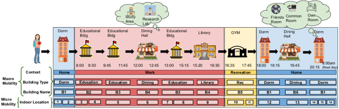
Figure 2. Mobility Hierarchical View

Multi-Scale Mobility While it has been shown that user mobility displays recurring patterns at a scale, we argue that human mobility is inherently hierarchical, where hierarchy is represented by spatial granularity scale as it becomes fine grained micro mobility from a coarse grained macro mobility representing context, building type, and building name. As shown in Figure 2, a user who visits several locations to accomplish their daily tasks seems extremely mobile at the scale of indoor location, visiting 14 locations throughout the day. As we change the spatial granularity to a coarser grain, we find that the mobility becomes infrequent at the building scale, where the user visits 10 buildings. Finally, at the context level—which defines the overall span of activities the user performs in the part of the day—the user shows mobility across only 4 contexts. Thus, showing that human mobility becomes more frequent as the spatial scale becomes fine grained. Also, each indoor location space shows high affinity to the context and building type displaying dependencies and correlations between macro and micro scale mobility features.

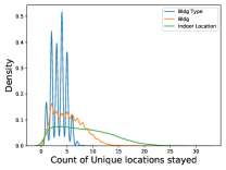
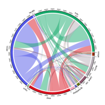
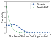
(a)	(b)	(c)

Figure 3. Features influencing indoor mobility prediction (a) Spatial Scale (b) Building Type (c) User Type

Features Impacting Indoor Mobility Prediction We conducted empirical analysis on a large campus WiFi syslog dataset described in §4 and found that four main factors impact micro mobility:

• Spatial Scale: Figure 3(a) is a density plot of count of dwell locations of users across an entire day at each spatial scale. Dwell location is defined as a location where users spend at least 10 minutes. Context describes the situational factors such as work or home. Building type indicates the building usage activity: for example, a food court is used for dining, while a building with classrooms is used for education. Building name is the location name visited, and the indoor location is the location inside the building visited as shown in Figure 2. We see that the average number of visits are 4, 5, and 11 at building type, building name, and indoor location level respectively. Giving us the insight that as the spatial scale becomes more fine-grained, from context to indoor mobility, the user mobility becomes more frequent.

• Building Type: Figure 3(b) is the chord diagram showing user movements within and across different building types. We see that an educational building, as well as dorms, see more dwell locations within the buildings where other building types such as admin, and dining see relatively less within building dwell locations. The main reason is that students move from one classroom to another within and across educational buildings during work hours resulting in a high number of dwell locations in education buildings. This indicates that the space type that governs the primary activity inside the building plays is an important feature in indoor human mobility.

• User Type: our campus dataset has two types of users, students, and faculty, as identified by the role field in the authentication events of syslog messages. Figure 3(c) shows the distribution of the unique number of buildings visited by users (students and faculty/staff), here multiple visits to a building count as a single unique location. We see that on an average a faculty/staff visits 1.2 unique buildings per day while students visit an average of  3 unique buildings per day. Thus, illustrating that user type influences the observed user mobility.

• Past Behavior: We find that the future mobility of a user is highly dependent on past behavior. Users who display high conformance behavior in the past continue to do so in the future. This observation is inline with the findings in prior work (Jayarajah and Misra, 2018).

2.1. Ethical Considerations

Our study has been approved by our Institutional Review Board (IRB) and is conducted under a Data Usage Agreement (DUA) with the campus network IT group that restricts and safeguards all the WiFi data collected. To avoid any privacy data leakage all the MAC ids and usernames in the syslogs are anonymized using a strong hashing algorithm. The hashing is performed before syslog data is stored on disk under the guidance of the IT manager who is the only person aware of the hash key of the algorithm. Any data analysis that results in the de-anonymization of the users is strictly prohibited under the IRB and signed DUA. All users using the campus WiFi network need to provide consent to the campus IT department for syslog data events from their devices to be stored for a system diagnosis or analysis of attacks on the enterprise network. Additionally, all researchers sign a form of consent to adhere to the signed IRB and DUA and undergo mandatory ethics training.

3. Problem and Approach

3.1. Problem Statement

We focus on the problem of modeling indoor mobility trajectories of users over the timescale of several hours to a day. We assume that historical indoor mobility data for each user is available for purposes of modeling. A trajectory of a user over a duration such as a day is defined to be a sequence of tuples (c,s,b,l), where each tuple comprises of context (c), space type (s), building location name (b) and indoor location name (l). Our model seeks to predict the trajectory of each user while learning the correlation between the c,s,b, and l at multiple spatial granularities. Further, we model trajectories inside a single building as well as those that span a collection of nearby buildings.

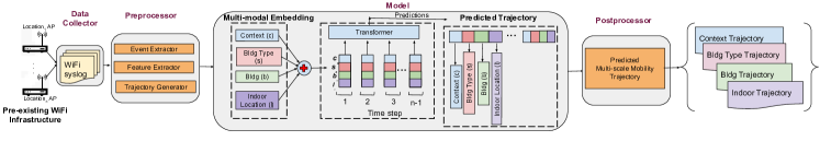
Figure 4. System Architecture Diagram

3.2. System Overview

Figure 4 shows the architectural overview of WiFiMod. WiFiMod is a pipeline of 3 main modules: data collector, data preprocessor, and model. The main objective of the data collector is to collect the WiFi syslog files across all the APs in the enterprise network. Most IT departments already have the networking logging turned on; if disabled then the IT admins would need to turn “on” the network logging to enable data collection. The output of this module is an aggregated syslog file from all APs across the campus. The aggregated syslog file is fed to the data preprocessor, which extracts the events and fields needed to generate user trajectories from the raw syslog files. This module is vendor-specific, depending on the vendor of the deployed AP. Currently, WiFiMod supports HP-Aruba syslog files. Once the user trajectories are extracted they are fed into the model, which extracts the macro and micro mobility features, creates a multi-modal feature embedding, and feeds it to the Transformer model. The output of the model are predictions, which can be used to generate reports or are aggregated to predict space usage and occupancy for various applications.

3.3. WiFi-Based Modeling Approach

A large, campus-like infrastructure comprises of various building types such as dormitory, educational, dining, student union, research labs, health center, recreational center and administrative. Campus users move across multiple buildings everyday to accomplish their tasks and use resources scattered across campus. A campus or enterprise WiFi network provides seamless WiFi coverage inside buildings and between buildings through Access Points (AP) installed across the geographical area of the institution. As users move within this geographical area, their devices connect and hop APs. Each AP maintains an internal log that consists of a list of all events observed by the AP.

When a user connects their device, it associates with a nearby AP. Each AP has a fixed location identified by the room, floor and building of installation. As a user moves across multiple locations on the campus, the device gets associated and disassociated with multiple APs on the user’s path. The association and disassociation events, along with timestamp, Device MAC, AP ID, and event type get logged in the internal syslog file maintained by each AP. Extracting all the association, disassociation or drift events from syslog files of all APs on the campus and indexing them by timestamp gives us a sequence of APs visited and duration of visit by each user device. Since all AP locations are known in terms of building, level and room of installation, it further helps us derive user device trajectory information at multiple spatial scales.

The enterprise WiFi network on campus is operated with RADIUS authentication that mandates all users to authenticate before connecting to the network. Since today’s users carry a plethora of mobile devices we extract these authorization messages from syslog files to create a user-to-device map and use this to identify the mobile devices (typically the smartphone) of each user and use its trajectory as an alias of the user trajectory.

Now, to train a data-driven model, we collect syslogs and extract trajectories for each user for a few weeks and create a historic trajectories dataset for training the model. From the extracted trajectories, we derive macro and micro mobility features based on the building type and heuristic rule for context defined above. This serves as the input to the model, which is a global model trained on all user trajectories. We use the multi-level spatial features of each trajectory to create a multi-modal embedding and train the Transformer. The predictions of this model are then used as is for individual mobility or can be aggregated.

3.4. System Architecture

3.4.1. Preprocessor:

The syslogs collected from the APs are a deluge of data mainly used for system diagnosis or analysis of attacks on the enterprise network. A typical syslog is a collection of diverse timestamped events, where each event has a pre-specified format. The goal of the preprocessor is to extract the relevant events from the syslog file and convert the events into a trajectory. The preprocessor is a sequence of 3 main steps: event extraction, data dependency resolution, and trajectory generator.

In the first step, we extract association, disassociation, reassociation, authorization, deauthorization, and drift event messages, hereby referred to as presence messages, from the syslog file. The event format is as shown below:

       <Timestamp> <hh:mm:ss> <controller_name> <event_id>
       <message_body : MAC_ID , AP_ID, other text>

The timestamp field gives us the time of event; $event\_id$ gives us the event type; $message\_body$ consists of device $MAC\_ID$, which identifies each device uniquely, and $AP\_ID$, which gives us the AP details namely building name, level and room number. Authorization and deauthorization messages additionally have username and role fields that help create a mapping between users and their devices, used for selecting the most mobile device from the collection of devices owned by each user, along with the role of the user on campus identified as student or faculty/staff.

The event logging in syslog has lots of inconsistencies such as dropped events, time sequence events overlap, multiple similar events, incorrect order of events, multiple disparate event types logged for the same device at the same timestamp, to name a few. Such inconsistencies need to be resolved before the mobility trajectory of the device aka user is computed. The main objective of this step is to resolve these inconsistencies, estimate the missing entries, clean the data, and generate a timestamped sequence of rows of association and disassociation of devices with AP.

After that, we gather all events per user device and create a timestamp indexed sequence to identify the APs visited, along with the time of visit, to generate a mobility trajectory. Then, for each generated indoor mobility trajectory, we add the corresponding context, building type, and building name to each visited indoor location. We generate the context based on a simple heuristic that campus working hours are between 8:30am and 4:30pm, so all user activities between these times are marked as ”work” context and the rest are marked as ”home” context. We find that students who stay on-campus display both these contexts whereas for off-campus users, we generally see only the work context except for students in research labs who work outside the work context hours and students who stay on campus to use recreation and student union facilities later or early during the day. Each building on our campus has a specific usage assigned to it (e.g. educational building have classrooms, dining has food courts, recreational building has swimming pools, squash courts, gymnasium). We use the designated space activity as the location space type. Thus, for each indoor location visited in the extracted WiFi trajectory we compute the corresponding context, space type, and building name resulting in a sequence of (c,s,b,l) tuple as the multiple spatial granularity trajectory.

3.4.2. Transformers for Sequential Prediction:

The Transformer neural network architecture (Vaswani et al., 2017), originally introduced for the task of machine translation, follows an encoder-decoder structure. The encoder maps a sequence of inputs $\bf{x}$ consisting of the inputs $x_{i}$ at each position $i$ to a sequence of continuous representations $\bf{z}$. These representations are provided as input to a decoder that autoregressively generates an output sequence of labels $\bf{y}$, with the prediction at each output timestep conditioned on the entire input sequence $\bf{z}$. The length of the output sequence is not tied to the length of the input sequence. In the Transformer architecture, the encoder and the decoder share the same neural network architecture structure, except that in the decoder, the representation at position $i$ is prevented from observing representations at subsequent positions. We describe this architecture in more detail below.

First, a sequence of input tokens is first mapped to corresponding $d_{model}$-dimensional input embeddings via an embedding lookup table. These embeddings are then fed to the encoder of the Transformer, which is comprised of $L$ layers of the same form. Each layer $j$ passes its inputs through two sub-layers, multi-head self-attention and a feed-forward layer, with residual connections (addition followed by normalization) between each:

$$h_{1} =MultiHeadAttention(\bf{x}^{(j-1)})$$

$$h_{2} =LayerNorm(\bf{x}^{(j-1)}+h_{1})$$

$$h_{3} =FeedForward(h_{2})$$

$$\bf{x}^{(j)} =LayerNorm(h_{2}+h_{3})$$

For the representation $x_{i}$ at a given position in the sequence, self-attention computes scores between $x_{i}$ and every other representation in $\bf{x}$, and uses those scores to compute a weighted average (attention) over the representations at all positions. In multi-head self-attention, this operation is performed $k$ times, so that $k$ different attention functions can be learnt, to model different dependencies between elements in the sequence. For more low-level details, see (Vaswani et al., 2017). For each attention head, three matrices $Q,K,V$ are created by multiplying the input (a sequence of embeddings) with weight matrices $W^{Q},W^{K},W^{V}$ (of dimension $d_{model}\times d_{model}$, $d_{model}\times d_{k}$, and $d_{model}\times d_{v}$, respectively). Using the terminology from (Vaswani et al., 2017), $Q$ represents ”queries”, $K$ represents ”keys”, and $V$ represents ”values”. The multi-head attention mechanism allows for the model to jointly attend to information from different representation subspaces along different positions. Layer normalization is applied after residual connections to improve optimization.

$$MultiHead(Q,K,V)=Concat(head_{1},...,head_{h})W^{o}$$

where,

$$head_{i}=Attention(QW_{i}^{Q},KW^{K}_{i},VW^{V}_{i})$$

Attention is given by the formula:

$$Attention(Q,K,V)=softmax\left(\frac{QK^{T}}{\sqrt[2]{d}_{k}}\right)V$$

It is also worth noting that, unlike recurrent neural networks (RNNs) or convolutional neural networks (CNNs), Transformers are not inherently sensitive to sequential order, and it is therefore common to inject information about the position of elements in the input sequence via positional encodings. These positional encodings are added to the input representations.

3.4.3. Multi-Modal Transformer Model:

To learn the sequential as well as long-term dependencies from the input trajectories we use a Transformer-based autoregressive (sometimes called ”causal”) language model. We use an off-the shelf Transformer implementation based on GPT-2 (Radford et al., 2019) and train it from scratch on our dataset. We treat the task of predicting the next set of locations visited by the user as a task of language modeling, where language modeling task is defined as the task of predicting next character or word in a document.

Our Transformer model takes as input $m=4$ trajectories corresponding to the context, space type, building, and indoor location spatial modalities generated by the preprocessor. We map the events in each raw trajectory to an index in a shared vocabulary of size $V$, to obtain $m$ integer-valued sequences $T_{1},...,T_{m}$, each with length $n$. Then, we map the entries in each sequence to learned, $d$-dimensional event embeddings $E_{1},...,E_{m}$, where $E_{i}=\langle e_{1},...,e_{n}\rangle$ and each $e_{i}\in\mathbb{R}^{d}$. Since the vocabulary is shared, we use a separate set of event embeddings for each modality to avoid collisions when event ids from different modalities happen to overlap. Since Transformer models inherently lack an inductive bias that would allow them to be sensitive to different sequential orderings, we also learn $d$-dimensional position embeddings $P$ for each of the $n$ positions. We obtain a single joint embedding by summing together $Je=E_{1}+...+E_{m}+P$. The derived joint embedding $Je$ is passed through $m$ stacked Transformer encoder layers, each of which has $m$ attention heads.

We train this model using a self-supervised autoregressive training objective: given the events at timesteps $1,...,i-1$ in each modality, the model is trained to predict the events that occur at timestep $i$. In other words, the model estimates $p(c_{i},s_{i},b_{i},l_{i}|c_{1:i-1},s_{1:i-1},b_{1:i-1},l_{1:i-1})$. To make predictions, we pass the outputs obtained from the Transformer encoder through an additional linear layer of dimension $d\times V$, which is shared across all modalities. We hypothesize that using a shared output layer encourages the embeddings for different modalities to maintain a coherent geometry relative to one another; however, we leave in-depth analysis of different architectural choices for future work.

During training, we convert the logits obtained from the output layer to (log) probabilities via the softmax function, then compute the batchwise-mean cross entropy loss for each modality. We sum these together to obtain a final combined loss. We minimize this objective over $15$ epochs using the Adam optimizer (Kingma and Ba, 2015) with a learning rate of $0.01$ and a mini-batch size of $100$. As mentioned above, we use $m=4$ Transformer layers and $m=4$ attention heads per layer. We set the embedding dimension $d$ to $64$.

4. Experimental Evaluation

4.1. Dataset and Parameter Setting

Dataset For the evaluation of our model we use campus-scale device trajectory dataset extracted from WiFi logs of a large university campus(name removed for double-blind review). Table 1 provides dataset details. Our campus comprises of 156 buildings spread over 1463 acres and has seamless wireless connectivity through 5104 HP Aruba access points (AP). These APs are managed by seven wireless controllers and they receive syslog messages of all events seen by the APs. AP logs contain many types of events, of which six events types are relevant to our study: association, disassociation, reassociation, authentication, de-authentication and drift events. Since the campus operates an enterprise WiFi network with RADIUS authentication, all user devices must authenticate themselves before they connect to the network. Doing so generates authentication and deauthentication log messages, which allows the network to associate each device with a particular user. Once authenticated, the device can then associate with a nearby access point, which generates an association message in the event logs. If the device moves out of range or wakes up from sleep, it may generate deassociation, reassociation or drift message. Each event in the log consists of a timestamp, device MAC ID and Access Point ID. In addition, authentication and deauthentication events also include the user ID. For privacy reasons, all device MAC ID and user ID are anonymized using a SHA-1 hash function as noted in section §2.1. Since the location of all access points are known (in terms of the building and floor where they are deployed), each of these event types represents a ”presence” message. The sequence of presence messages generated by a device over the course of the day reveals all the AP (and building-specific) locations visited by that device and the time spent at each location. Further, since each device must first authenticate to the network with the user ID for RADIUS authentication, the owner of each device is known, which in turn reveals the collection of devices owned by each user. As noted earlier, this data has been collected, and anonymized, under an IRB protocol approved by our Institutional Review Board. We remove stationary network devices identified by association with a single AP for the entire dataset duration and select only the most mobile device (smartphone) as an alias for the user mobility. Identification of devices owned by each user and selection of only the most mobile device as alias of user mobility helps avoid double counting users as well. For evaluation of WiFiMod we use event log for the 2 months of Fall’19 is over 150GB in size and contains 6.4 billion events.

Item Description	Value
Number of Users	2000
Number of Building Types	13
Number of Buildings	156
Number of APs	5104
Avg. Buildings visited	4
Avg. Indoor locations stayed	8.97/building
Time Span	Fall’19: Sep-Nov ’19

Table 1. Dataset Description

Parameter Setting: To evaluate the robustness of our proposed model we use a train-dev-test split of 80-10-10 where we use the first 80% data of each user as training data, next 10% as dev and rest 10% as testing data. For the selection of model hyper-parameters, we use a grid search over the parameter space and select the optimal parameter settings using the dev dataset. Parameter optimization is performed using mini-batch Adam optimizer and with a batch size of 100.

4.2. Baseline Comparison

To evaluate the effectiveness of our model we compare our proposed model with the following:

N-gram: An n-gram model is one of the most important tools in speech, language and text processing. An n-gram model is used to estimate the conditional probability of visiting a location given the sequence of previously visited locations. We include evaluations against first and second order Markov chains as the baseline. A bi-gram model uses past location to estimate the probabilities (using MLE), whereas tri-gram approach conditions on past 2 locations.

HMM: In a Hidden Markov Model (HMM) we regard all visited locations as state and build a transition matrix based on the sequence of locations visited. We train one HMM for all users and each hidden state generates locations over a Gaussian distribution.

LSTM Long Short Term Memory (LSTM) has shown superior performance for sequential data and encoding long term dependencies, so we use LSTM as one of our baselines.

Simple Transformer is an adaption of our model, which does not perform multi-modal embedding. For indoor modeling we train the simple transformer with the historic indoor trajectories. It is a basic autoregressive language model implemented with Transformers.

Model Name	15 mins	30 mins	60 mins
bi-gram	5.32%	6.24%	7.94%
tri-gram	9.51%	12 .3%	19.24%
four-gram	14.45%	17.5%	24.8%
HMM	15.16%	20.21%	25.36%
LSTM	57.48%	62.3%	71.96%
Simple Transformer	64.28%	69.93%	75.81%
Our Model	68.39%	79.4%	83.2%

Table 2. WiFiMod indoor mobility prediction comparison with Baseline Models.

Results: Table 2 shows the comparison results between our proposed model and the baseline models. For the evaluation, we predict the entire indoor trajectory generated by each model for each user at a temporal granularity of 15 mins, 30 mins, and 60 mins and check the predictions against the ground-truth locations to compute the model accuracy. We evaluate WiFiMod against other baselines and find that Transformer-based WiFiMod outperforms both the LSTM model and HMM. Transformers have a higher-order transition modelling capacity than a HMM. In addition, the multi-head self-attention mechanism allows it to capture long-term dependencies more effectively than an LSTM.

In general, the deep neural network (DNN) based models show superior performance to n-gram models and HMMs, demonstrating that long-term historic information is important for mobility modeling and prediction. The DNN approach captures long-term regularities—e.g. if the start location of a trajectory is a dormitory, the likelihood of the trajectory ending in the same dormitory is high—whereas this information is not captured by n-gram or HMM models.

Additionally, we observe that, due to variations in human behavior, there are errors in prediction too. For example, students frequently change the dining halls visited based on the menu at each dining hall or based on the dining location visited by their friends. Also, non-regular mobility such as visits to university health center or to an administrative office are hard to predict and the model does not capture such high variations from users’ routine mobility. We also find that our model captures the recurring mobility patterns at the inter-building level with a very high accuracy of  90% but, due to variations introduced by human behavior such as visiting a different dining hall or carrying out an unexpected errand at an administrative building, etc results in the induction of errors. Another interesting observation is that varying the temporal scale of trajectory has an impact on the prediction accuracy.

Impact of Temporal Granularity In this experiment, we vary the temporal granularity of training and prediction. Trajectory temporal granularity refers to the sampling rate of trajectories. We represent the user trajectory as a sequence of locations, where the location is sampled every $n$ minutes. We train the model on trajectories with a temporal granularity of 15 mins, 30 mins, and 60 mins, here on referred to as T15, T30, and T60 respectively. As shown in Table 2, we find that across all models with different sampling frequency T60 prediction is highest followed by T30 and then T15. We find that as the model temporal granularity becomes coarser, the indoor mobility accuracy increases because indoor human mobility is more frequent at fine granularity. When we learn mobility at a coarser temporal scale of 60 mins, frequent short mobility observed at 15 min temporal scale such as a break to visit the vending machine or stop by a colleague’s office for a chat gets masked. Additionally, such short micro events have high variability and cannot be predicted accurately at a fine temporal granularity resulting in reduced accuracy at a fine temporal granularity as seen in T15 trajectories ,location sampled every 15 mins.

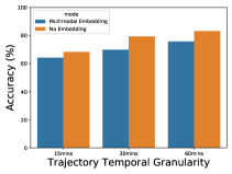
Figure 5. Multimodal embedding effectiveness : Comparison of indoor location prediction of a transformer for multimodal and non-multimodal embedding input

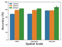
Figure 6. Space Type Prediction

4.3. Effectiveness of Multi-Modal Embedding

In figure 5 we see that the indoor mobility prediction accuracy of our model is higher than a single Transformer implementation that has a flat input structure of only indoor locations. To compare the two models on prediction accuracy, we predict the next top-1 location with both the models for the same test dataset on indoor location granularity. The multi-modal embedding model shows an accuracy of 83.2% while a simple transformer with no embedding has an accuracy of 75.81% for T60 trajectories. The multi-modal embedding approach outperforms the non-embedding approach even for T15 and T30 trajectories demonstrating that modeling mobility from a hierarchical perspective where the model learns the correlations across multiple spatial scale mobility using multi-modal embedding results in higher prediction accuracy. The intuition behind higher accuracy is that the multi-modal approach significantly reduces the prediction space by learning the correlations between macro and micro scale mobility, conditioning the prediction on the estimated macro and micro scale mobility distribution, thereby using the topological constraint of the multiple spatial scales. This behaviour is also reflected in Table 3, which compares the accuracy of hierarchical and non-hierarchical model across multiple spatial scales. Additionally, the model also captures the correlation and periodicity in mobility across varying spatial scales.

Spatial Scale	WiFiMod	Non-Hierarchical
Building Type	89.58%	89.23%
Building Name	87.39%	81.12%
Indoor Location	83.2%	75.81%

Table 3. Comparison of accuracy of hierarchical and non-hierarchical model across multiple spatial scale.

4.4. Importance of Space Type Prediction

While analyzing the indoor location predictions made by the model, we find that most of the errors are in predicting food court location and space inside food courts, indoor library locations of use, indoor location inside the recreation center, etc. These locations have a high variance when predicting the indoor location. However, we find that the model displays a high accuracy in predicting the context, and location types and low accuracy on building name, in the case of multiple food courts, or indoor location of use. Figure 6 analyzes the model accuracy by space type. We see that the model has high prediction accuracy for building type followed by building name and lowest for indoor location across all 3 sampling frequencies T15, T30, and T60. This is mainly because, while routine activities such as visiting the classrooms, office space, research labs have fixed building type, building name, and indoor location while visits to high variance locations such as library or dining hall has a fixed building type but variance in indoor locations (since the person might not sit at the same location always) and building name (since the person might not visit the same building under the building type, such as dining hall). Additionally, we find that most errors are found in indoor location prediction, fine spatial granularity for high sampling rate of 1 sample every 15 mins in T15 because this trajectory captures the most unscheduled high variance micro mobility at a fine spatial scale.

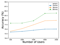
Figure 7. Impact of number of users on model accuracy

4.5. Impact of the number of trajectories

We vary the training dataset by using a subset of trajectories, with subset sizes of 500,1000,1500,2000, and 2500 user trajectories. We train the models on the subset of user trajectories for the first 7 weeks of the semester and predict the user trajectories for the next 2 weeks. We find that the transformer based model displays higher accuracy for larger training set size indicating that the model has better generalizability and higher performance for more and new data. The model accuracy for T15 increases the most from 73.4% to 75.06%, whereas model accuracy for T60 increases from 78.28% to 83.2% . Across all trajectories, with different temporal binning we see that the model accuracy increases as we increase the number of user trajectories in the training dataset.

5. Case Studies

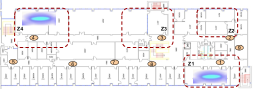
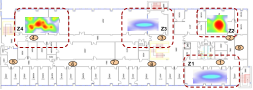
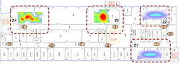
(a) 8:30am	(b) 12:00pm(Noon)	(c) 3:30pm

Figure 8. Heatmap of predicted indoor occupancy of educational bldg with classrooms, research labs, faculty office, kitchenette

In this section we discuss three case studies of our proposed system WiFiMod .

5.1. Casestudy 1: Indoor COVID19/ILI Hotspot Prediction

With the current COVID-19 pandemic, building occupancy scheduling and resource allocation for de-densification is a key component in designing re-opening policies. Here, we present a case study of using WiFiMod to predict indoor mobility of a building across the coarse of an entire day(s) to identify indoor spaces with high space utilization that can become a hot pocket zone and needs dedensification so that the number of users inside the building is always below the 50% or 25% usage constraint for space usage..

Here, we use the trained model to predict the user trajectories of all users on campus for the entire day. We then aggregate all these predicted trajectories across the temporal attribute to compute the occupancy at each indoor location at various times of the day. In our case since we are using WiFi AP syslogs, the indoor spatial granularity is zone level where each AP captures occupancy per zone that might encapsulate a single room or across few rooms, based on the range of AP deployed. Fig 8 shows the floor map of an educational building with 9 deployed APs. The floor has a combination of faculty office, break room, research labs, and classrooms. We focus on APs 1-4 which have a range across zones Z1-Z4 respectively as indicated in figure 8. Zone Z1 encompasses few faculty offices and a research lab, Z2 spans across a kitchenette and a research lab, Z3 across a conference room and a student work space, and Z4 across a classroom and a research lab. Fig 8 (a)-(d) shows the computed indoor user occupancy based on the model predictions, at 3 different times of the day. We find that at 8:30am fig 8(a) the space occupancy is very low with the start of the day across all zones, with some occupancy in Z1 and Z4. Fig 8(b) shows predicted space occupancy at noon and we observe high human density across Z4(classroom zone) with an in-person class (in 2019), Z2(kitchenette area) with the break room where students gather to eat lunch, and the rest zones show low to moderate occupancy. Fig 8(c) shows predicted space usage at 3pm and we see that zones Z3, and Z4 have high occupancy due to predicted recurring seminar, and classroom usage respectively while Z2 kitchennet and Z1 lab space have relatively low occupancy. Fig 8(d) shows predicted space usage at 5pm and we see some occupancy in zones Z1 and Z2 that comprise of research labs with students still working in late evenings. The computed occupancy across the 3 times of the day shows an accuracy of 96% as compared with observed ground truth indoor occupancy computed from WiFi logs.

In the heatmaps 8(a)-(c) the red areas indicate high human density or hotpocket zones on the floor map. We can generate such heatmaps for all indoor spaces across the times of the day to identify hotpockets and design policies or space usage schedules to de-densify them to lower the risk of disease spread and safe opening of indoor spaces.

Additionally, indoor location occupancy computed by aggregating indoor mobility can also be used to generate customized Heating, Ventilation, and Air Conditioning (HVAC) schedules per building. Such customized HVAC schedules can help reduce the energy consumption while increasing the user comfort by scheduling HVAC to turn-on with predicted indoor occupancy while turning it off with low to no indoor occupancy.

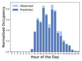
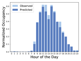
(a) Location1(r2 0.989)	(b) Location2(r2 0.984)

Figure 9. Normalized hourly occupancy across 2 locations computed from actual and simulated trajectories.

5.2. Casestudy 2: Human Mobility Simulation

Mobility datasets are fundamental to evaluation of a system or applications such as simulation of disease spread. However, such datasets are hard to obtain due to privacy concerns. Majority of the mobility trajectory generators use deterministic models that have predefined mobility distributions or assume human mobility follows levy walk, random distribution or stochastic process, failing to capture realistic mobility. This leads to a gap in analyzing and fine tuning systems. Hence, we propose scenario simulation by generating synthetic mobility trace using our pre-trained hierarchical model. To demonstrate the efficacy of our model for synthetic trace generation we generate the trajectory of users and their devices using a pre-trained model on the campus mobility dataset. We compare the hourly occupancy at 2 different locations computed from the synthetic trace and observed trajectories. The simulation is performed at 20% of the total population, and the observed transition and occupancy are scaled down accordingly. Figure  9(a) and (b) compares the hourly occupancy of 2 different locations, loc1 and loc2, and the model demonstrates a high accuracy with the coefficient of determination, r² value as 0.989 and 0.984 for the loc1 and loc2 respectively.

For applications such as user profiling and behaviour analysis, which need to capture variations in human behavior we can introduce realism in capturing the variations in human behavior by changing the inference mechanism in the decoder from selecting the next location that gives least negative log-likelihood to sampling the next location from the top-5 possible next predictions. To validate if our synthetic traces are close to the real dataset, we do a domain search of the generated trace to actual observed trace and find trajectory similarity score of 82% on weekdays and 63% on weekends for indoor mobility.

5.3. Casestudy 3: Single User Personal Assistant

Last few years have seen an introduction of personal assistants that share the goal of presenting the user the right information at the right time. However, knowing when to present the information without any query from the user is an important criterion and a critical limitation in many of today’s models. Since, the information presented is mainly associated with current location, time of day, space type, and user type. We propose that a user mobility model derived by using WiFiMod serves as a foundation for a highly accurate personal assistant that can be used for informing users with a variety of tasks/events/updates. We use a globally trained model and fine tune it for each user by locally training it with the historic trajectories of each user to create a personalized model and use it to make macro and micro scale predictions. We find that our model shows high indoor mobility prediction accuracy in the top-1(accuracy of most likely location) prediction score is  89% for user type faculty/staff and  85% for user type student for weekdays. Such a model can be augmented with the user calendar or campus event calendar to notify the user with upcoming events of interest or prior scheduled classes or meetings.

6. Related Work

There has been significant work on using Markov Models or Hidden Markov Models (HMMs) to capture the sequential nature of human mobility. However, capturing long-term dependence in the data or recurring patterns is challenging when using Markov Models; doing so requires the use of higher-order Markov models, which quickly grow in complexity and computational overheads.

Most of the mobility modeling work focusses on outdoor mobility modeling at urban-scales (Isaacman et al., 2012; Lin et al., 2017; Lee and Hou, 2006; Kim et al., 2006) , next location prediction (Do and Gatica-Perez, 2012; Liu et al., 2016; Lin et al., 2012; Gambs et al., 2012; Gidófalvi and Dong, 2012; Mathew et al., 2012), and point of interest areas (Yuan et al., 2012) using a variety of data sources such as cellular, WiFi, social media check-ins, and vehicular data (Ganti et al., 2013; Hang et al., 2018; Veloso et al., 2011; Hasan et al., 2013; Jurdak et al., 2015). All these outdoor models cater to a discrete mobility models where mobility is infrequent compared to fine grain indoor mobility hence these outdoor models cannot be directly applied to indoor environments.

More recent work in this area has focused on urban mobility modeling using cellular, transportation or social media data using data driven methods, specifically deep learning. Recurrent Neural Networks (RNNs) have emerged as a popular approach for urban mobility modeling (Lin et al., 2017; Feng et al., 2018; Song et al., 2016; Zhang et al., 2018; Jiang et al., 2018) taking inspiration from Natural Language Processing (NLP) to learn long term dependencies. ST-RNN model (Al-Molegi et al., 2016) models spatial and temporal contexts of mobility but is too complicated with the need to tune a lot of parameters and cannot be easily deployed for indoor mobility which is very frequent. In DeepMove (Feng et al., 2018) the authors propose using RNN to model sparse trajectories. It does not cater to either indoor mobility or capturing the mutli-scale hierarchical mobility correlations.

Other efforts in indoor mobility modeling comprise of (Jayarajah and Misra, 2018) but this approach is for modeling mobility based on groups and social friendship ties. Additionally they use aaa to acquire the dataset and it requires human effort and cost in acquisition. WiFiMod uses passively sensed WiFi syslogs and doesn’t need any new infrastructure or human feedback for data collection. There has been work on using WiFi probes for sensing where the probe requests from mobile devices that steadily scan the APs close by for access are used for monitoring the crowds or activity flow for monitoring users (Xi et al., 2014; Weppner et al., 2016). These prior works do not focus on individual mobility and instead look at crowd and activity behavior of aggregated users. In our work we focus on individual user mobility trajectories using WiFi syslogs and not WiFi probes. Additionally, our model supports all applications that need individual as well as aggregated human mobility unlike only aggregated behavior as analyzed by prior work.

7. Conclusions

Modeling indoor mobility and using the correct spatial granularity of mobility can substantially benefit a large range of applications. In this paper, we proposed WiFiMod, a data-driven approach to model indoor human mobility using passively sensed WiFi logs. In WiFiMod we jointly model mobility context, space type, outdoor location, and indoor location using a transformer to learn the correlations of mobility at various spatial granularities. We extensively evaluated our approach using available ground truth WiFi data from 2500 users at a large university campus and found that our model outperforms the current state-of-the-art baselines significantly. Further, we also demonstrated the need and use of modeling mobility at multiple spatial scales. Additionally, we demonstrated that our proposed approach can be applied to many other real-world applications such as Personal assistant design, trajectory simulation, and indoor human density or hot pocket prediction to help with resource allocation, scheduling, as well as COVID19 de-densification policy compliance among many others.

References

- (1)
- Al-Molegi et al. (2016) Abdulrahman Al-Molegi, Mohammed Jabreel, and Baraq Ghaleb. 2016. STF-RNN: Space Time Features-based Recurrent Neural Network for predicting people next location. In 2016 IEEE Symposium Series on Computational Intelligence (SSCI). IEEE, 1–7.
- Arif et al. (2016) Mohammed Arif, Martha Katafygiotou, Ahmed Mazroei, Amit Kaushik, Esam Elsarrag, et al. 2016. Impact of indoor environmental quality on occupant well-being and comfort: A review of the literature. International Journal of Sustainable Built Environment 5, 1 (2016), 1–11.
- Camp et al. (2002) Tracy Camp, Jeff Boleng, and Vanessa Davies. 2002. A survey of mobility models for ad hoc network research. Wireless communications and mobile computing 2, 5 (2002), 483–502.
- Davies et al. (2000) Vanessa Ann Davies et al. 2000. Evaluating mobility models within an ad hoc network. Master’s thesis. Citeseer.
- Do and Gatica-Perez (2012) Trinh Minh Tri Do and Daniel Gatica-Perez. 2012. Contextual Conditional Models for Smartphone-based Human Mobility Prediction. In Proceedings of the 2012 ACM Conference on Ubiquitous Computing (UbiComp ’12). ACM, New York, NY, USA, 163–172. https://doi.org/10.1145/2370216.2370242
- Feng et al. (2018) Jie Feng, Yong Li, Chao Zhang, Funing Sun, Fanchao Meng, Ang Guo, and Depeng Jin. 2018. DeepMove: Predicting Human Mobility with Attentional Recurrent Networks. In Proceedings of the 2018 World Wide Web Conference (WWW ’18). International World Wide Web Conferences Steering Committee, Republic and Canton of Geneva, Switzerland, 1459–1468. https://doi.org/10.1145/3178876.3186058
- Gambs et al. (2012) Sébastien Gambs, Marc-Olivier Killijian, and Miguel Núñez del Prado Cortez. 2012. Next place prediction using mobility markov chains. In Proceedings of the First Workshop on Measurement, Privacy, and Mobility. ACM, 3.
- Ganti et al. (2013) Raghu Ganti, Mudhakar Srivatsa, Anand Ranganathan, and Jiawei Han. 2013. Inferring Human Mobility Patterns from Taxicab Location Traces. In Proceedings of the 2013 ACM International Joint Conference on Pervasive and Ubiquitous Computing (UbiComp ’13). ACM, New York, NY, USA, 459–468. https://doi.org/10.1145/2493432.2493466
- Gidófalvi and Dong (2012) Győző Gidófalvi and Fang Dong. 2012. When and where next: individual mobility prediction. In Proceedings of the First ACM SIGSPATIAL International Workshop on Mobile Geographic Information Systems. ACM, 57–64.
- Hang et al. (2018) Mengyue Hang, Ian Pytlarz, and Jennifer Neville. 2018. Exploring student check-in behavior for improved point-of-interest prediction. In Proceedings of the 24th ACM SIGKDD International Conference on Knowledge Discovery & Data Mining. ACM, 321–330.
- Hasan et al. (2013) Samiul Hasan, Xianyuan Zhan, and Satish V Ukkusuri. 2013. Understanding urban human activity and mobility patterns using large-scale location-based data from online social media. In Proceedings of the 2nd ACM SIGKDD international workshop on urban computing. ACM, 6.
- Huang et al. (2010) Lian Huang, Qingquan Li, and Yang Yue. 2010. Activity identification from GPS trajectories using spatial temporal POIs’ attractiveness. In Proceedings of the 2nd ACM SIGSPATIAL International Workshop on location based social networks. ACM, 27–30.
- Isaacman et al. (2012) Sibren Isaacman, Richard Becker, Ramón Cáceres, Margaret Martonosi, James Rowland, Alexander Varshavsky, and Walter Willinger. 2012. Human mobility modeling at metropolitan scales. In Proceedings of the 10th international conference on Mobile systems, applications, and services. ACM.
- Jayarajah and Misra (2018) Kasthuri Jayarajah and Archan Misra. 2018. Predicting episodes of non-conformant mobility in indoor environments. Proceedings of the ACM on Interactive, Mobile, Wearable and Ubiquitous Technologies 2, 4 (2018), 1–24.
- Jiang et al. (2018) Renhe Jiang, Xuan Song, Zipei Fan, Tianqi Xia, Quanjun Chen, Qi Chen, and Ryosuke Shibasaki. 2018. Deep ROI-Based Modeling for Urban Human Mobility Prediction. Proceedings of the ACM on Interactive, Mobile, Wearable and Ubiquitous Technologies 2, 1 (2018), 14.
- Jurdak et al. (2015) Raja Jurdak, Kun Zhao, Jiajun Liu, Maurice AbouJaoude, Mark Cameron, and David Newth. 2015. Understanding human mobility from Twitter. PloS one 10, 7 (2015), e0131469.
- Kim et al. (2006) Minkyong Kim, David Kotz, and Songkuk Kim. 2006. Extracting a mobility model from real user traces. In INFOCOM 2006. 25th IEEE International Conference on Computer Communications. Proceedings. IEEE, 1–13.
- Kingma and Ba (2015) Diederik P. Kingma and Jimmy Lei Ba. 2015. Adam: A method for stochastic optimization. 3rd International Conference on Learning Representations, ICLR 2015 - Conference Track Proceedings (2015), 1–15. arXiv:1412.6980 https://arxiv.org/pdf/1412.6980.pdf
- Lee and Hou (2006) Jong-Kwon Lee and Jennifer C. Hou. 2006. Modeling Steady-state and Transient Behaviors of User Mobility: Formulation, Analysis, and Application. In Proceedings of the 7th ACM International Symposium on Mobile Ad Hoc Networking and Computing (MobiHoc ’06). ACM, New York, NY, USA, 85–96. https://doi.org/10.1145/1132905.1132915
- Liao et al. ([n.d.]) Dongliang Liao, Weiqing Liu, Yuan Zhong, Jing Li, and Guowei Wang. [n.d.]. Predicting Activity and Location with Multi-task Context Aware Recurrent Neural Network. In Proceedings of the 27th International Joint Conference on Artificial Intelligence (IJCAI’18).
- Lin et al. (2012) Miao Lin, Wen-Jing Hsu, and Zhuo Qi Lee. 2012. Predictability of Individuals’ Mobility with High-resolution Positioning Data. In Proceedings of the 2012 ACM Conference on Ubiquitous Computing (UbiComp ’12). ACM, New York, NY, USA, 381–390. https://doi.org/10.1145/2370216.2370274
- Lin et al. (2017) Ziheng Lin, Mogeng Yin, Sidney Feygin, Madeleine Sheehan, Jean-Francois Paiement, and Alexei Pozdnoukhov. 2017. Deep generative models of urban mobility. IEEE Transactions on Intelligent Transportation Systems (2017).
- Liu et al. (2016) Qiang Liu, Shu Wu, Liang Wang, and Tieniu Tan. 2016. Predicting the Next Location: A Recurrent Model with Spatial and Temporal Contexts.. In AAAI. 194–200.
- Mathew et al. (2012) Wesley Mathew, Ruben Raposo, and Bruno Martins. 2012. Predicting future locations with hidden Markov models. In Proceedings of the 2012 ACM conference on ubiquitous computing. ACM, 911–918.
- Qiao et al. (2018) Yuanyuan Qiao, Zhongwei Si, Yanting Zhang, Fehmi Ben Abdesslem, Xinyu Zhang, and Jie Yang. 2018. A hybrid Markov-based model for human mobility prediction. Neurocomputing 278 (2018), 99–109.
- Radford et al. (2019) Alec Radford, Jeffrey Wu, Rewon Child, David Luan, Dario Amodei, and Ilya Sutskever. 2019. Language Models are Unsupervised Multitask Learners. arXiv (2019). https://github.com/codelucas/newspaper
- Song et al. (2010) Chaoming Song, Tal Koren, Pu Wang, and Albert-László Barabási. 2010. Modelling the scaling properties of human mobility. Nature physics 6, 10 (2010), 818–823.
- Song et al. (2016) Xuan Song, Hiroshi Kanasugi, and Ryosuke Shibasaki. 2016. DeepTransport: Prediction and Simulation of Human Mobility and Transportation Mode at a Citywide Level.. In IJCAI, Vol. 16. 2618–2624.
- Vaswani et al. (2017) Ashish Vaswani, Noam Shazeer, Niki Parmar, Jakob Uszkoreit, Llion Jones, Aidan N Gomez, Lukasz Kaiser, and Illia Polosukhin. 2017. Attention is all you need. arXiv preprint arXiv:1706.03762 (2017).
- Veloso et al. (2011) Marco Veloso, Santi Phithakkitnukoon, and Carlos Bento. 2011. Urban mobility study using taxi traces. In Proceedings of the 2011 international workshop on Trajectory data mining and analysis. ACM, 23–30.
- Weppner et al. (2016) Jens Weppner, Benjamin Bischke, and Paul Lukowicz. 2016. Monitoring crowd condition in public spaces by tracking mobile consumer devices with wifi interface. In Proceedings of the 2016 ACM International Joint Conference on Pervasive and Ubiquitous Computing: Adjunct. 1363–1371.
- Wolf et al. (2020) Thomas Wolf, Lysandre Debut, Victor Sanh, Julien Chaumond, Clement Delangue, Anthony Moi, Pierric Cistac, Tim Rault, Rémi Louf, Morgan Funtowicz, Joe Davison, Sam Shleifer, Patrick von Platen, Clara Ma, Yacine Jernite, Julien Plu, Canwen Xu, Teven Le Scao, Sylvain Gugger, Mariama Drame, Quentin Lhoest, and Alexander M. Rush. 2020. Transformers: State-of-the-Art Natural Language Processing. In Proceedings of the 2020 Conference on Empirical Methods in Natural Language Processing: System Demonstrations. Association for Computational Linguistics, Online.
- Xi et al. (2014) Wei Xi, Jizhong Zhao, Xiang-Yang Li, Kun Zhao, Shaojie Tang, Xue Liu, and Zhiping Jiang. 2014. Electronic frog eye: Counting crowd using WiFi. In IEEE INFOCOM 2014-IEEE Conference on Computer Communications. IEEE, 361–369.
- Yuan et al. (2012) Jing Yuan, Yu Zheng, and Xing Xie. 2012. Discovering regions of different functions in a city using human mobility and POIs. In Proceedings of the 18th ACM SIGKDD international conference on Knowledge discovery and data mining. ACM, 186–194.
- Zhang et al. (2018) Hanyuan Zhang, Hao Wu, Weiwei Sun, and Baihua Zheng. 2018. Deeptravel: a neural network based travel time estimation model with auxiliary supervision. arXiv preprint arXiv:1802.02147 (2018).
- Zheng et al. (2018) Zimu Zheng, Feng Wang, Dan Wang, and Liang Zhang. 2018. Buildings Affect Mobile Patterns: Developing a New Urban Mobility Model. In Proceedings of the 5th Conference on Systems for Built Environments (BuildSys ’18). ACM, New York, NY, USA, 83–92. https://doi.org/10.1145/3276774.3276780
- Zhou et al. (2017) Mengyu Zhou, Dan Pei, Kaixin Sui, and Thomas Moscibroda. 2017. Mining crowd mobility and WiFi hotspots on a densely-populated campus. In Proceedings of the 2017 ACM International Joint Conference on Pervasive and Ubiquitous Computing and Proceedings of the 2017 ACM International Symposium on Wearable Computers. ACM, 427–431.