Gaussian process regression: Optimality, robustness, and relationship with kernel ridge regression

Abstract

Gaussian process regression is widely used in many fields, for example, machine learning, reinforcement learning and uncertainty quantification. One key component of Gaussian process regression is the unknown correlation function, which needs to be specified. In this paper, we investigate what would happen if the correlation function is misspecified. We derive upper and lower error bounds for Gaussian process regression with possibly misspecified correlation functions. We find that when the sampling scheme is quasi-uniform, the optimal convergence rate can be attained even if the smoothness of the imposed correlation function exceeds that of the true correlation function. We also obtain convergence rates of kernel ridge regression with misspecified kernel function, where the underlying truth is a deterministic function. Our study reveals a close connection between the convergence rates of Gaussian process regression and kernel ridge regression, which is aligned with the relationship between sample paths of Gaussian process and the corresponding reproducing kernel Hilbert space. This work establishes a bridge between Bayesian learning based on Gaussian process and frequentist kernel methods with reproducing kernel Hilbert space.

1 Introduction

Gaussian process regression is widely applied in machine learning (Rasmussen and Williams,, 2006), including reinforcement learning (Rasmussen et al.,, 2003) and Bayesian optimization (Shahriari et al.,, 2016; Frazier,, 2018; Bull,, 2011; Klein et al.,, 2017); spatial statistics (Cressie,, 2015; Stein,, 1999; Matheron,, 1963); computer experiments (Santner et al.,, 2003; Sacks et al.,, 1989), and many others, to capture the intrinsic randomness of the underlying function. The goal of Gaussian process regression is to recover an underlying function based on noisy observations. As a Bayesian machine learning method, the key idea of Gaussian process regression is to impose a probabilistic structure, which is a Gaussian process, on the underlying truth. Based on this assumption, the conditional distribution at each unobserved point in the interested domain is normal with explicit mean and variance. The conditional mean provides a natural predictor of the function value, and the pointwise confidence interval constructed based on the conditional variance can be used for statistical uncertainty quantification.

In this work, we establish error bounds on Gaussian process regression, where the smoothness of the correlation function can be misspecified, and the observations have noise. We consider that the underlying truth is a Gaussian process, which is a standard setting in Gaussian process modeling (Stein,, 1999; Santner et al.,, 2003; Gramacy,, 2020). Although the noisy observations have been extensively considered in the setting that the underlying truth is a deterministic function (Wynne et al.,, 2021; Steinwart et al.,, 2009; Fischer and Steinwart,, 2020; van der Vaart and van Zanten,, 2011, and references therein), (see Section 2 for more discussions), it is somewhat surprising that there has been little study on this in the literature when the underlying truth is a Gaussian process. The difference is that, the convergence results for a deterministic function usually depend on some quantities related to the underlying function (e.g., the norm of the underlying function in some function space), while for a Gaussian process, these quantities themselves may be random. Thus, the convergence for a Gaussian process regression needs to be analyzed with a different approach. We derive prediction lower and upper error bounds under $L_{2}$ metric and with fixed design. Specifically, we show that if the smoothness of the true correlation function is $m_{0}$ and the smoothness of the imposed correlation function lies in $[m_{0},\infty)$, with an appropriate regularization parameter and quasi-uniform design points, the convergence rate under $L_{2}$ metric is $n^{-(m_{0}-d/2)/(2m_{0})}$, where $d$ is the dimension and $n$ is the sample size. Furthermore, we prove that this convergence rate is optimal under certain assumptions. Our theory can be applied to justifying the use of space-filling designs, where the design points spread approximately evenly in the region of interest, since quasi-uniform designs are space-filling designs. If the smoothness of the imposed correlation function, denoted by $m$, is less than $m_{0}$, we show that the convergence rate of upper error bound is $n^{-(m-d/2)/(2m)}$.

Here, we should keep in mind not to confuse the setting of Gaussian process regression with the settings of other fields, including nonparametric regression (Gu,, 2013; van de Geer,, 2000) and posterior contraction of Gaussian process priors (van der Vaart and van Zanten, 2008a, ; van der Vaart and van Zanten,, 2011). The hypothesis spaces are different in the later two fields. In particular, the underlying function is assumed to be deterministic, which leads to different notions of smoothness and convergence rates (Kanagawa et al.,, 2018; Tuo and Wang,, 2020).

We also consider one popular kernel method: kernel ridge regression, where the reproducing kernel Hilbert space can be misspecified. This is a frequentist approach, where the underlying truth is assumed to be a deterministic function. The reason for considering kernel ridge regression is two-fold.

First, the study paves the way to establish the intriguing relationship between Gaussian process regression and kernel ridge regression with more details given later. At first sight, the two areas are very different, for example, completely different approaches have been employed to investigate their convergence rates respectively. On the other hand, the two areas share some striking similarities in certain aspects, for example, their predictors take rather similar forms, and also their model assumptions bear strong resemblance. A thorough review on the differences and connection of Gaussian process and reproducing kernel Hilbert space can be found in Kanagawa et al., (2018). Therefore, it is natural to ask whether there are some deep relationships between Gaussian process regression and kernel ridge regression. Kanagawa et al., (2018) provides a positive answer. Remark 5.5 of Kanagawa et al., (2018) states a theoretical equivalence between Gaussian process regression and kernel ridge regression, where the Gaussian process regression model and the convergence rate (Kanagawa et al.,, 2018, Theorem 5.1) is based on the posterior contraction of Gaussian process priors in van der Vaart and van Zanten, (2011). Although the underlying truth in van der Vaart and van Zanten, (2011) is still a deterministic function, Remark 5.5 of Kanagawa et al., (2018) reveals a relationship between Gaussian process regression and kernel ridge regression. Based on the constructed convergence rate in Gaussian process regression, we conduct a further investigation and establish a relationship based on the situations where “the underlying truth in Gaussian process regression is a Gaussian process” and “the underlying truth in kernel ridge regression is a deterministic function”.

We now describe briefly their relationship, which is summarized in Figure 1. If the true correlation function has smoothness $m_{0}$, then the sample paths of the Gaussian process have a smoothness $m_{0}-d/2$, but do not lie in the Sobolev space $H^{m_{0}-d/2}$ with a strictly positive probability (Steinwart,, 2019; Kanagawa et al.,, 2018). For a deterministic function $f$ with smoothness $m_{0}(f)=m_{0}-d/2$, the optimal convergence rate is $n^{-m_{0}(f)/(2m_{0}(f)+d)}=n^{-(m_{0}-d/2)/(2m_{0})}$, which coincides with the optimal convergence rate of Gaussian process regression. Furthermore, the optimal value of the regularization parameter in kernel ridge regression coincides with that of the regularization parameter in Gaussian process regression. In other words, we can regard Gaussian process regression as kernel ridge regression with an oversmoothed kernel function shifted by a smoothness $d/2$, from prediction perspective. This coincidence reveals an interesting relationship between kernel ridge regression and Gaussian process regression, and provides more insights on the connection between these two methods.

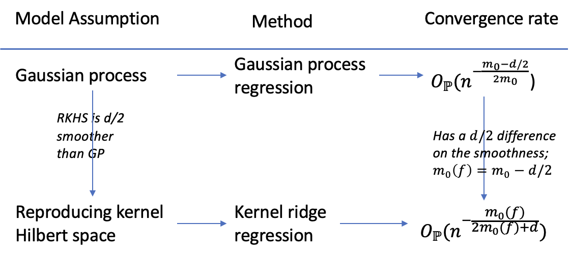
Figure 1: Relationship between the convergence rates of oversmoothed Gaussian process regression ($m_{0}\leq m<\infty$) and kernel ridge regression. We use the following abbreviation. RKHS: Reproducing kernel Hilbert space; GP: Gaussian process.

Second, we will derive some new and interesting results on convergence rates, which complements the existing literature on this topic. Specifically, suppose $f$ has smoothness $m_{0}(f)$, and the corresponding Sobolev space with smoothness $m_{0}(f)$ is denoted by $H^{m_{0}(f)}$. We show that the kernel ridge regression can still achieve the optimal convergence rate, if the corresponding reproducing kernel Hilbert space is associated with a smoothness lying in $[m_{0}(f)/2,\infty)$. If $f\in H^{m_{0}(f)}$, this recovers the convergence results in the misspecified kernel ridge regression literature (e.g., Blanchard and Mücke, (2018); Dicker et al., (2017); Guo et al., (2017); Lin et al., (2017); Steinwart et al., (2009); Fischer and Steinwart, (2020)), while the settings are different. See Section 2.2 for detailed discussion. Nevertheless, we note that if a function has smoothness $m_{0}(f)$, it may not lie in the corresponding Sobolev space with smoothness $m_{0}(f)$; examples include triangle function and Matérn kernel functions; see Section 5.1.1. We are not aware of any work related to the convergence rate under the scenario $f\notin H^{m_{0}(f)}$ but has smoothness $m_{0}(f)$. Table 1 summarizes the results obtained in this work. For the briefness, we assume the design is quasi-uniform in Table 1, and present general results in the main text.

Method	Model Assumption	Convergence rate
Gaussian process	$f$ is a realization of	$O_{\mathbb{P}}(n^{-\frac{2m_{0}-d}{2m_{0}}})$ (optimal rate),	$O_{\mathbb{P}}(n^{-\frac{2m-d}{2m}})$,
regression	a Gaussian process $Z$.	for $m_{0}\leq m<\infty$.	for $m\leq m_{0}$.
Kernel ridge	$f$ is a deterministic	$f\in H^{m_{0}(f)}$: $O_{\mathbb{P}}(n^{-\frac{m_{0}(f)}{2m_{0}(f)+d}})$,	$O_{\mathbb{P}}(n^{-\frac{2m}{4m+d}})$,
regression	function.	$f\notin H^{m_{0}(f)}$: $O_{\mathbb{P}}(n^{-\frac{m_{0}(f)}{2m_{0}(f)+d}}Q(n))$,	for $m<m_{0}(f)/2$.
		for $m_{0}(f)/2\leq m<\infty$.

Table 1: Summary of the $L_{2}$ convergence rates of misspecified Gaussian process regression and kernel ridge regression. The function $Q$ satisfies $\lim_{s\rightarrow+\infty}(\log Q(s))/(\log s)=0$. The two rates on the shaded row were presented in previous literature, while our settings and mathematical development are different.

The rest of this paper is arranged as follows. We first make comparison to related works in Section 2. In Section 3, we introduce some preliminaries. In Section 4, we provide convergence rates of misspecified Gaussian process regression. In Section 5, we discuss the relationship between the convergence rates of misspecified Gaussian process regression and kernel ridge regression, where we also present convergence rates of misspecified kernel ridge regression. Numerical experiments are conducted in Section 6. Conclusions and discussion are made in Section 7. Technical proofs are provided in Appendix.

2 Related literature

In this subsection, we first remark some differences between our results and previous works. The previous works can be roughly divided into two fields: Gaussian process modeling, where the underlying truth is assumed to be a Gaussian process, and deterministic function reconstruction, where the underlying truth is modeled as a deterministic function. The difference between the convergence rate analysis in these two settings is that, in deterministic function reconstruction, the convergence rate usually involves some kind of function norm of the underlying true function, while for Gaussian process modeling, this norm itself is also random, which needs to be further considered. Although our work focuses on the Gaussian process modeling, we also consider the kernel ridge regression and obtain some interesting results. We utilize mathematical tools from both fields in the present work. For example, Lemma E.1 comes from Gaussian process modeling, and the rate of convergence of kernel ridge regression is established based on the previous works Tuo et al., (2020); van de Geer, (2000). Moreover, mathematical tools in scattered data approximation (Wendland,, 2004) play an important role in our analysis.

2.1 Gaussian process modeling

The rate of convergence of Gaussian process regression without noise has been studied in much literature, see Buslaev and Seleznjev, (1999); Yakowitz and Szidarovszky, (1985); Stein, 1990b for example, where the convergence rate is pointwise or the input points are not general scattered data points. Recent works Wang et al., (2020); Tuo and Wang, (2020) study the rate of convergence of Gaussian process regression in the $L_{p}(\Omega)$ norm, with $1\leq p\leq\infty$ under different designs and misspeficied correlation functions in the noiseless case. To the best of our knowledge, the only work that studies Gaussian process regression with noisy observations is Lederer et al., (2019). In Lederer et al., (2019), a uniform error bound of Gaussian process regression has been provided, where the unknown realization $f$ and the correlation function are assumed to have a Lipschitz continuity, and the noise is normal. Furthermore, the correlation function in Lederer et al., (2019) is well-specified.

In this work, we study the rate of convergence of Gaussian process regression in the $L_{2}(\Omega)$ norm, under different designs and misspeficied correlation functions, but we take the noise into consideration. These settings differentiate our work with the previous works in Gaussian process modeling.

2.2 Deterministic function reconstruction

Comparing with Gaussian process modeling, there are much more literature studying the deterministic function reconstruction. The most related fields to the present work are kernel ridge regression, posterior contraction of Gaussian process priors, and scattered data approximation.

Kernel ridge regression

Although we focus on the Gaussian process regression, we also consider the kernel ridge regression and obtain some interesting results. We consider that $f$ has smoothness $m_{0}(f)$, in the sense that is to be introduced later in Section 5.1.1. If the underlying true function $f\in H^{m_{0}(f)}$, we recover the convergence rates obtained by Blanchard and Mücke, (2018); Dicker et al., (2017); Guo et al., (2017); Lin et al., (2017); Steinwart et al., (2009), while the model settings are different. Specifically, the design points in the above works are random. Moreover, the assumptions are different. The aforementioned works impose conditions on the eigenvalues and eigenfunctions (Blanchard and Mücke,, 2018; Dicker et al.,, 2017; Guo et al.,, 2017; Lin et al.,, 2017; Steinwart et al.,, 2009; Fischer and Steinwart,, 2020).

The aforementioned works have different model settings from our work, which provides some additional insights on the study of kernel ridge regression. Specifically, we adopt model settings similar to Tuo et al., (2020), where the widely used Matérn kernel functions can be used and the design points are fixed. These model settings allow us to consider the case that the underlying function $f\notin H^{m_{0}(f)}$ but has smoothness $m_{0}(f)$. We employ the empirical process technique together with Fourier transform to derive the convergence rates. Following this approach, we do not need to make assumptions on the eigenvalues and eigenfunctions, but we need additional conditions on the interested region. Moreover, our results show the advantage of space-filling designs.

Posterior contraction of Gaussian process priors

In this field, despite the use of Gaussian process priors, the underlying function is still assumed to be deterministic. An incomplete list of papers in this area includes Castillo, (2008, 2014); Giordano and Nickl, (2019); Nickl and Söhl, (2017); Pati et al., (2015); van der Vaart and van Zanten, (2011); van der Vaart and van Zanten, 2008a ; van Waaij and van Zanten, (2016). We are not aware of any error bounds in this area in terms of our settings, i.e., fixed designs, fill and separation distances.

Scattered data approximation

In the field of scattered data approximation, the goal is to approximate or interpolate an underlying deterministic function. Examples include Wendland, (2004); Wendland and Rieger, (2005); Rieger and Zwicknagl, (2009); Narcowich et al., (2006), which cover the noiseless case, and Wynne et al., (2021); Rieger and Zwicknagl, (2009), which cover the case that the observations have noise. The misspecification case is considered in Narcowich et al., (2006); Wynne et al., (2021). Although the observations are corrupted by noise in Wynne et al., (2021); Rieger and Zwicknagl, (2009) as we considered in the present work, the convergence rates are different. If one plugs in our settings into their bounds, it can be seen that the prediction error bound does not converge to zero. This is the price for the more general noise assumption in Wynne et al., (2021); Rieger and Zwicknagl, (2009). We impose the sub-Gaussian assumption (see Condition (C5) in Section 3.2) and obtain a sharper error bound.

3 Preliminaries

In this section, we introduce problem settings and conditions.

3.1 Problem settings

Suppose that our observations $(x_{k},y_{k})$ satisfy the following model

$$y_{k}=f(x_{k})+\epsilon_{k},k=1,...,n,$$ (3.1)

where $x_{k}\in\Omega\subset\mathbb{R}^{d}$ and $\epsilon_{k}\overset{\text{i.i.d.}}{\sim}(0,\sigma_{\epsilon}^{2})$, i.e., independent and identically distributed random noise with mean zero and variance $\sigma_{\epsilon}^{2}$. In Gaussian process regression, the underlying function $f$ is assumed to be a realization of a Gaussian process $Z$. From this point of view, we shall not differentiate $f$ and $Z$ in Gaussian process regression. We assume $Z$ is a zero-mean stationary Gaussian process, denoted by $Z\sim GP(0,\sigma^{2}\Psi)$, with $\text{Cov}(Z(x),Z(x^{\prime}))=\sigma^{2}\Psi(x-x^{\prime})$ for $x,x^{\prime}\in\mathbb{R}^{d}$. Here $\sigma^{2}$ is the variance, and $\Psi$ is the ture but typically unknown correlation function which is stationary, positive definite and integrable on $\mathbb{R}^{d}$.

For a moment, assume $\epsilon_{k}$’s are normal. Given the correlation function $\Psi$ and conditional on $Y=(y_{1},...,y_{n})^{T}$, $Z(x)$ is normally distributed at an unobserved point $x$. The conditional expectation and variance of $Z(x)$ are given by

$$\mathbb{E}[Z(x)|Y]= r(x)^{T}(R+\mu I_{n})^{-1}Y,$$ (3.2)

$$\text{Var}[Z(x)|Y]= \sigma^{2}(\Psi(x-x)-r(x)^{T}(R+\mu I_{n})^{-1}r(x)),$$ (3.3)

where $r(x)=(\Psi(x-x_{1}),\ldots,\Psi(x-x_{n}))^{T},R=(\Psi(x_{j}-x_{k}))_{jk}$, $I_{n}$ is an identity matrix, and $\mu=\sigma_{\epsilon}^{2}/\sigma^{2}$. The conditional expectation (3.2) is a natural predictor of $Z(x)$, and it can be shown that the conditional expectation is indeed the best linear predictor (Ankenman et al.,, 2010), in the sense that it has the minimal mean squared prediction error (MSPE), which equals $\text{Var}[Z(x)|Y]$.

In this work, we investigate what happens if another correlation function $\Phi$, referred to as the imposed correlation function, is used in Gaussian process regression in place of the true correlation function $\Psi$. The resulting Gaussian process regression predictor after using $\Phi$ is

$$\widehat{f}_{G}(x)=r_{m}(x)^{T}(R_{m}+\mu_{m}I_{n})^{-1}Y,\quad x\in\Omega,$$ (3.4)

where $r_{m}(x)=(\Phi(x-x_{1}),\ldots,\Phi(x-x_{n}))^{T}$ and $R_{m}=(\Phi(x_{j}-x_{k}))_{jk}$. We suppose $\mu_{m}$ is chosen according to our will and call it the regularization parameter. Clearly, $\widehat{f}_{G}$ in (3.4) is no longer the best linear unbiased predictor. In this work, we are interested in the $L_{2}$ prediction error using the imposed correlation function $\Phi$, i.e.,

$$\|Z-\widehat{f}_{G}\|_{L_{2}(\Omega)}.$$ (3.5)

Similar problem without the influence of noise has been considered in Tuo and Wang, (2020). Other convergence results of Gaussian process regression with misspecified correlation functions can be found in Stein, (1988); Stein, 1990a ; Stein, 1990b ; Tuo and Wang, (2020); Wang et al., (2020); Yakowitz and Szidarovszky, (1985), where the observations are noiseless. However, the appearance of noise can significantly change the analysis of convergence when the underlying truth is a Gaussian process, as we will see later.

3.2 Notation and conditions

In the rest of this work, the following definitions are used. For two positive sequences $a_{n}$ and $b_{n}$, we write $a_{n}\asymp b_{n}$ if, for some $C,C^{\prime}>0$, $C\leq a_{n}/b_{n}\leq C^{\prime}$. Similarly, we write $a_{n}\gtrsim b_{n}$ if $a_{n}\geq Cb_{n}$ for some constant $C>0$, and $a_{n}\lesssim b_{n}$ if $a_{n}\leq C^{\prime}b_{n}$ for some constant $C^{\prime}>0$. Also, $C,C^{\prime},c_{j},C_{j},j\geq 0$ are generic positive constants, of which value can change from line to line. We use $Q(s)$ to denote an increasing positive function satisfying

$$\lim_{s\rightarrow+\infty}\frac{\log Q(s)}{\log s}=0$$ (3.6)

and not depending on $n$, which may vary at each occurrence. The Euclidean metric is denoted by $\|\cdot\|_{2}$. The Fourier transform of $f\in L_{1}(\mathbb{R}^{d})$ is given by

$$\mathcal{F}(f)(\omega)=(2\pi)^{-d/2}\int_{\mathbb{R}^{d}}f(x)e^{-ix^{T}\omega}dx.$$

The following conditions will be assumed throughout the paper, unless otherwise specified.

1. The region of interest $\Omega\subset\mathbb{R}^{d}$ is a compact set with positive Lebesgue measure and Lipschitz boundary, and satisfies an interior cone condition, i.e., there exist $\alpha\in(0,\pi/2)$ and $\mathcal{R}>0$ such that for every $x\in\Omega$, a unit vector $\xi(x)$ exists such that the cone $\mathcal{C}(x,\xi(x),\alpha,\mathcal{R}):=\left\{x+\lambda y:y\in\mathbb{R}^{d},\|y\|=1,y^{T}\xi(x)\geq\cos\alpha,\lambda\in[0,\mathcal{R}]\right\}$ is contained in $\Omega$.

2. There exists $m_{0}>d/2$ such that,

   $$c_{1}(1+\|\omega\|_{2}^{2})^{-m_{0}}\leq\mathcal{F}(\Psi)(\omega)\leq c_{2}(1+\|\omega\|_{2}^{2})^{-m_{0}},\forall\omega\in\mathbb{R}^{d}.$$

3. There exists $m>d/2$ such that,

   $$c_{3}(1+\|\omega\|_{2}^{2})^{-m}\leq\mathcal{F}(\Phi)(\omega)\leq c_{4}(1+\|\omega\|_{2}^{2})^{-m},\forall\omega\in\mathbb{R}^{d}.$$

4. Let $\mathcal{X}=\{X_{1},X_{2},...\}$ be a sequence of designs. Without loss of generality, assume that ${\rm card}(X_{n})=n$, where $n$ takes its value in an infinite subset of $\mathbb{N}$, and card$(X)$ denote the cardinality of set $X$. We call $\mathcal{X}$ a sampling scheme. The fill distance of $X_{n}$, defined by

   $$h_{X_{n},\Omega}=\sup_{x\in\Omega}\inf_{x_{j}\in X_{n}}\|x-x_{j}\|_{2},$$ (3.7)

   satisfies

   $$h_{X_{n},\Omega}\leq Cn^{-1/d},\forall n\geq 1.$$

5. (Sub-Gaussian) Suppose $\epsilon_{k}$’s in (3.1) are independent and identically distributed random variables satisfying

   $$C^{2}(\mathbb{E}e^{|\epsilon_{k}|^{2}/C^{2}}-1)\leq C^{\prime},\quad k=1,...,n.$$

   Such random variables are called sub-Gaussian (van de Geer,, 2000).

Condition (C1) is a geometric condition on the region $\Omega$. We believe it holds in most practical situations, because the compactness and convexity imply the interior cone condition; see Hofmann et al., (2007); Niculescu and Persson, (2006).

Conditions (C2) and (C3) imply that the Fourier transforms of the true correlation function and imposed correlation function have an algebraical decay. A prominent class of correlation functions that have an algebraical decay of their Fourier transforms is the (isotropic) Matérn correlation functions. The isotropic Matérn correlation functions (Stein,, 1999) is defined by

$$\Psi_{M}(x;\phi,\nu)=\frac{1}{\Gamma(\nu)2^{\nu-1}}(2\sqrt{\nu}\phi\|x\|_{2})^{\nu}K_{\nu}(2\sqrt{\nu}\phi\|x\|_{2}),$$ (3.8)

with the Fourier transform (Tuo and Wu,, 2016)

$$\mathcal{F}(\Psi_{M})(\omega;\nu,\phi)=4^{\nu+\frac{d}{2}}\pi^{\frac{d}{2}}\frac{\Gamma(\nu+\frac{d}{2})}{\Gamma(\nu)}(\nu\phi^{2})^{\nu}(4\nu\phi^{2}+\|\omega\|_{2}^{2})^{-(\nu+\frac{d}{2})},$$ (3.9)

where $\phi>0$ is the scale parameter, and $K_{\nu}$ is the modified Bessel function of the second kind. The parameter $\nu$ is the smoothness parameter, which is associated with the smoothness of the kernel function $\Psi_{M}$.

Another example of correlation functions with algebraically decayed Fourier transforms is the generalized Wendland correlation function (Wendland,, 2004; Gneiting,, 2002; Chernih and Hubbert,, 2014; Bevilacqua et al.,, 2019; Fasshauer and McCourt,, 2015), defined as

$$\Psi_{GW}(x)=\left\{\begin{array}[]{lc}\frac{1}{B(2\kappa,\eta+1)}\int_{\|\phi x\|}^{1}u(u^{2}-\|\phi x\|^{2})^{\kappa-1}(1-u)^{\eta}du,&0\leq\|x\|<\frac{1}{\phi},\\ 0,&\|x\|\geq\frac{1}{\phi},\end{array}\right.$$

where $\phi,\kappa>0$ and $\eta\geq(d+1)/2+\kappa$, and $B$ denotes the beta function. See Theorem 1 of Bevilacqua et al., (2019).

In this work, we consider fixed designs, where the design points $x_{1},...,x_{n}$ are fixed and can be chosen according to our will. Fixed designs are widely used in the field of computer experiments (Santner et al.,, 2003). Such designs include quasi-uniform designs (Borodachov et al.,, 2007; Utreras,, 1988), maximin Latin hypercube designs (Van Dam et al.,, 2007), optimal Latin hypercube designs (Park,, 1994), and grid points. Condition (C4) states that the fill distance of designs can be controlled at a certain rate. It can be seen that any quasi-uniform sampling scheme satisfies Condition (C4), as stated in the following example.

Definition 3.1 (Separation radius).

For $X=\{x_{1},...,x_{n}\}$, define the separation radius as

$$q_{X}=\min_{1\leq j\neq k\leq n}\|x_{j}-x_{k}\|_{2}/2.$$ (3.10)

Example 3.2 (Quasi-uniform designs).

It is easy to check that $h_{X,\Omega}\geq q_{X}$ (Wendland,, 2004) for any set of points $X$. A sampling scheme $\mathcal{X}=\{X_{1},X_{2},\ldots\}$ is called quasi-uniform if $h_{X_{n},\Omega}/q_{X_{n}}\leq C$ for all $n$. For a quasi-uniform sampling scheme, $h_{X_{n},\Omega}\asymp q_{X_{n}}\asymp n^{-1/d}$ (Müller,, 2009).

Obviously, a sampling scheme satisfying Condition (C4) may not be quasi-uniform. For example, we can add a point which is very close to one design point of a quasi-uniform design such that the separation radius is close to zero, and $h_{X_{n},\Omega}/q_{X_{n}}\leq C$ does not hold.

Remark 1.

Random samplings do not satisfy Condition (C4); see Example 1 of Tuo and Wang, (2020).

4 Rates of convergence for misspecified Gaussian process regression

In this section, we present our results on the convergence rate of the prediction error of misspecified Gaussian process regression (3.5).

We start with the easiest case. If the imposed correlation function is the same as the true correlation function, i.e., $\Phi=\Psi$ and $\mu_{m}=\sigma_{\epsilon}^{2}/\sigma^{2}$, then $\widehat{f}_{G}$ is the best linear predictor and achieves the minimal MSPE, which is $\text{Var}[Z(x)|Y]$; see Section 3.1. Obviously, the best linear predictor achieves the optimal convergence rate for a sampling scheme $\mathcal{X}=\{X_{1},X_{2},...\}$. It can be shown that if $\mu_{m}$ is any fixed positive constant and $\Phi=\Psi$, the optimal convergence rate can still be achieved.

Proposition 4.1.

Let $\widehat{f}_{G}(x)$ be as in (3.4) with $\Phi=\Psi$ and $\mu_{m}=C$, where $C>0$ is any fixed constant. For any fixed design $X=\{x_{1},...,x_{n}\}\subset\Omega$,

$$\mathbb{E}(\widehat{f}_{G}(x)-Z(x))^{2}\leq C_{1}\sigma^{2}(\Psi(x-x)-r(x)^{T}(R+\mu I_{n})^{-1}r(x))=C_{1}\text{Var}[Z(x)|Y]$$

holds for all $x\in\Omega$, where $R$, $r(x)$ and $\mu$ are as in (3.2), and the constant $C_{1}$ only depends on $C$, $\sigma_{\epsilon}^{2}$ and $\sigma^{2}$.

The proof of Proposition 4.1 can be found in Appendix C. Because $\text{Var}[Z(x)|Y]$ is the minimal MSPE, $\mathbb{E}(\widehat{f}_{G}(x)-Z(x))^{2}\geq\text{Var}[Z(x)|Y]$. Proposition 4.1 shows that if the true correlation function is used, the regularization parameter can be changed to any fixed constant and would not influence the optimal convergence rate. However, Proposition 4.1 does not provide any assertion on the convergence rate.

In the following, we provide several error bounds of misspecified Gaussian process regression under noisy observations. Suppose that $\Psi$ and $\Phi$ satisfy Condition (C2) and Condition (C3), respectively. If $m_{0}<m<\infty$, we call this case oversmoothed case and call the corresponding imposed correlation function $\Phi$ oversmoothed correlation function. On the other hand, if $d/2<m<m_{0}$, we call this case undersmoothed case and call the corresponding imposed correlation function $\Phi$ undersmoothed correlation function. If $m=m_{0}$, we call this case well-specified case.

We first provide an upper bound on the term $\Psi(x-x)-r(x)^{T}(R+\mu_{1}I_{n})^{-1}r(x)$ in the following proposition, which is closely related to the conditional variance in (3.3). The proof of Proposition 4.2 is provided in Appendix D. Proposition 4.2 plays a key role in the proofs of Theorems 4.3 and 4.5.

Proposition 4.2.

Suppose Conditions (C1)-(C4) hold. Then we have for any positive constant $\mu_{1}\gtrsim n^{1-2m_{0}/d}$,

$$\Psi(x-x)-r(x)^{T}(R+\mu_{1}I_{n})^{-1}r(x)\lesssim(\mu_{1}/n)^{1-\frac{d}{2m_{0}}},$$ (4.1)

where $r(x)$ and $R$ are as in (3.2).

Remark 2.

Proposition 4.2 is a deterministic version of Lemma F.8 in Wang, (2020). In Proposition 4.2, the design points are fixed, while in Lemma F.8 of Wang, (2020), the design points are uniformly distributed on $\Omega$.

Remark 3.

Note that when the observations are noisy, the convergence rate of the conditional variance (3.3) can be directly obtained by setting $\mu_{1}=\mu$, where $\mu$ is as in (3.2). This result is different with the existing results in scattered data approximation (Wendland,, 2004; Wu and Schaback,, 1993), where the observations have no noise.

We start with the oversmoothed case. In the following theorem, we assume that both the true correlation function $\Psi$ and the imposed correlation function $\Phi$ are Matérn correlation functions as in (3.8). Recall that $h_{X,\Omega}$ and $q_{X}$ are the fill distance and separation radius for a design $X$ as defined in (3.7) and (3.10), respectively. The proof of Theorem 4.3 is in Appendix E.

Theorem 4.3 (Oversmoothed Matérn correlation function).

Let $\Psi$ and $\Phi$ be two Matérn correlation functions as in (3.8). Suppose Conditions (C1)-(C5) hold. Suppose $m_{0}\leq m<\infty$ and $\mu_{m}\gtrsim n^{1-\frac{2m}{d}}$. Then, for any $t_{1},t_{2}\geq C_{0}$ and all $n$, with probability at least $1-\exp(-t_{1}^{2})-\exp(-t_{2}^{2})$, we have

$$\|Z-\widehat{f}_{G}\|_{L_{2}(\Omega)}^{2}\leq C\left((1+t_{1})^{2}T+t_{2}^{2}\mu_{m}^{-\frac{d}{2m}}n^{-\left(1-\frac{d}{2m}\right)}\right),$$

where $T=\mu_{m}^{-\frac{m-m_{0}}{m}}q_{X_{n}}^{-\frac{(m-m_{0})d}{m}}(\mu_{m}/n)^{1-\frac{d}{2m}}+\mu_{m}^{\frac{2m_{0}-d}{2m}}q_{X_{n}}^{\frac{(2m_{0}-d)d}{2m}}$, and the constants $C,C_{0}$ do not depend on $n$, $t_{1}$ and $t_{2}$.

The following corollary states that, if a sampling scheme is quasi-uniform, then Gaussian process regression with an oversmoothed Matérn correlation function can still lead to the error bound $O_{\mathbb{P}}(n^{-\frac{2m_{0}-d}{2m_{0}}})$. Recall that a sampling scheme $\mathcal{X}=\{X_{1},X_{2},\ldots\}$ is said to be quasi-uniform if $h_{X_{n},\Omega}/q_{X_{n}}\leq C$ for all $n$ (see Example 3.2). Corollary 4.4 is a direct result of Theorem 4.3 and the proof is omitted.

Corollary 4.4 (Oversmoothed Matérn correlation function and quasi-uniform design).

Let $\Psi$ and $\Phi$ be two Matérn correlation functions as in (3.8). Suppose Conditions (C1)-(C3) and (C5) hold. Suppose $m_{0}\leq m<\infty$ and the sampling scheme $\mathcal{X}$ is quasi-uniform. Let $\mu_{m}\asymp n^{-m/m_{0}+1}$. Then, for all $t\geq C_{0}$ and $n$, with probability at least $1-\exp(-t)$, we have

$$\|Z-\widehat{f}_{G}\|_{L_{2}(\Omega)}^{2}\leq C(1+t)n^{-\frac{2m_{0}-d}{2m_{0}}},$$

where $C_{0}$ and $C$ are constants not depending on $n$ and $t$. In particular, we have

$$\|Z-\widehat{f}_{G}\|_{L_{2}(\Omega)}^{2}=O_{\mathbb{P}}(n^{-\frac{2m_{0}-d}{2m_{0}}}).$$

Now we consider Gaussian process regression with undersmoothed correlation functions. The following theorem indicates that the convergence rate is slower than that of Gaussian process regression with oversmoothed correlation functions, whose proof is provided in Appendix F. Note that in Theorem 4.5, the true and imposed correlation functions are not necessarily Matérn correlation functions.

Theorem 4.5 (Undersmoothed correlation function).

Suppose Conditions (C1)-(C5) hold. Suppose $d/2<m\leq m_{0}$ and $\mu_{m}\gtrsim n^{1-\frac{2m}{d}}$. Then, for any $t_{1},t_{2}\geq C_{0}$ and $n$, with probability at least $1-\exp(-t_{1}^{2})-\exp(-t_{2}^{2})$, we have

$$\|Z-\widehat{f}_{G}\|_{L_{2}(\Omega)}^{2}\lesssim t_{1}^{2}\mu_{m}^{-\frac{d}{2m}}n^{-\left(1-\frac{d}{2m}\right)}+(1+t_{2})^{2}(\mu_{m}/n)^{1-\frac{d}{2m}}.$$

In particular, if $\mu_{m}$ is a fixed constant, $\|Z-\widehat{f}_{G}\|_{L_{2}(\Omega)}^{2}=O_{\mathbb{P}}(n^{-\frac{2m-d}{2m}})$.

The following corollary provides error bounds in the well-specified case. Corollary 4.6 is a direct result of Theorem 4.5, and the proof is omitted.

Corollary 4.6 (Well-specified correlation function).

Suppose Conditions (C1)-(C5) hold. Furthermore, suppose $m=m_{0}$ and $\mu_{m}\asymp 1$. Then, for all $t\geq C_{0}$ and $n$, with probability at least $1-\exp(-t)$, we have

$$\|Z-\widehat{f}_{G}\|_{L_{2}(\Omega)}^{2}\leq C(1+t)n^{-\frac{2m_{0}-d}{2m_{0}}},$$

where $C_{0}$ and $C$ are constants not depending on $n$ and $t$. In particular, $\|Z-\widehat{f}_{G}\|_{L_{2}(\Omega)}^{2}=O_{\mathbb{P}}(n^{-\frac{2m_{0}-d}{2m_{0}}}).$

Theorem 4.7 provides a lower error bound of Gaussian process regression, whose proof is presented in Appendix G.

Theorem 4.7 (Lower error bounds of Gaussian process regression).

Suppose Conditions (C1)-(C5) hold. Assume $m_{0}>d$ and Assumption G.0.1 holds. Then we have

$$\mathbb{E}\|Z-\widehat{f}_{G}\|_{L_{2}(\Omega)}^{2}\gtrsim n^{-\frac{2m_{0}-d}{2m_{0}}}.$$

Remark 4.

Theorem 4.7 requires a technical assumption Assumption G.0.1 in Appendix G, which essentially requires that there exists a correlation function $K$ with uniformly bounded eigenfunctions such that $\mathcal{F}(K)/\mathcal{F}(\Psi)$ is uniformly bounded. This assumption is slightly weaker than the assumption that $\Psi$ has uniformly bounded eigenfunctions. The later assumption is typical in nonparametric regression literature. See Mendelson et al., (2010); Steinwart et al., (2009) for example. Unfortunately, to the best of our knowledge, whether Assumption G.0.1 holds for Matérn correlation functions is not present in literature.

Remark 5.

Note that the convergence rate in Theorem 4.7 is different with the minimax convergence rate in nonparameteric regression, where the underlying truth is a deterministic function. Besides the different settings, another difference is that the minimax convergence rate is considered in the worst case for a given function class, while Theorem 4.7 can be treated as in an average case. We also note that Tuo and Wang, (2020) provide lower error bounds of Gaussian process regression in the noiseless case.

Combining Theorem 4.7 and Corollary 4.4, it can be seen that Gaussian process regression with an oversmoothed Matérn correlation function achieves the optimal convergence rate, if the sampling scheme is quasi-uniform, and the optimal convergence rate for Gaussian process regression is $O_{\mathbb{P}}(n^{-\frac{2m_{0}-d}{2m_{0}}})$. Corollary 4.6 states that the optimal convergence rate can also be achieved if the Gaussian process regression with the true correlation function is used, which is intuitively true.

Theorem 4.5 provides an upper bound on the $L_{2}$ prediction error of Gaussian process regression with an undersmoothed correlation function. The upper bound is larger than that of the Gaussian process regression with the true correlation function. Note that in Tuo and Wang, (2020) and Wang et al., (2020), if the observations have no noise, it has been shown that using an oversmoothed Matérn correlation function and a quasi-uniform sampling scheme can achieve the optimal convergence rate, while using an undersmoothed correlation function leads to an upper bound that has a slower convergence rate. Combining their results and ours, we can conclude that if the sampling scheme is quasi-uniform, using oversmoothed correlation functions is not detrimental to the convergence rate, no matter the observations are corrupted by noise or not. Nevertheless, we still recommend practitioners to try to find the correlation function with smoothness closed to the true smoothness. This is because the constant in the convergence rate can be large if the imposed smoothness is too far away from the true smoothness. Moreover, our results suggest that it is important to choose good designs in practice.

5 Relationship of the convergence rates between Gaussian process regression and kernel ridge regression

In this section, we discuss the relationship between the convergence rates of Gaussian process regression and kernel ridge regression. For the conciseness of this paper, we move the introduction to reproducing kernel Hilbert spaces, Sobolev spaces, and kernel ridge regression to Appendix A.

5.1 Rates of convergence for misspecified kernel ridge regression

5.1.1 Smoothness of a deterministic function

We say that a deterministic function $g\in L_{2}(\mathbb{R}^{d})$ has a finite degree of smoothness if the quantity

$$m_{0}(g):=\sup\{k\geq 0:g\in H^{k}(\mathbb{R}^{d})\}$$ (5.1)

is finite, where $H^{k}(\mathbb{R}^{d})$ is the Sobolev space with smoothness $k$. Here $k$ can be a non-integer, and the corresponding Sobolev space is called the fractional Sobolev space. We call the quantity (5.1) the smoothness of $g$. The functions considered in this work are assumed to have smoothness greater than $d/2$, which implies such function are continuous. Since $\Omega$ is compact and has a Lipschitz boundary, there exists an extension operator from $L_{2}(\Omega)$ to $L_{2}(\mathbb{R}^{d})$, such that the smoothness of each function is maintained (DeVore and Sharpley,, 1993; Rychkov,, 1999). We define the smoothness of a function $g\in L_{2}(\Omega)$ by the smoothness of the extended function $g_{e}\in L_{2}(\mathbb{R}^{d})$ using (5.1).

From (5.1), it can be seen that a function $g$ with smoothness $m_{0}(g)$ can be divided into two scenarios: 1) $g\in H^{m_{0}(g)}(\Omega)$ but $g\not\in H^{m}(\Omega)$ for any $m>m_{0}(g)$; 2) $g\in H^{m}(\Omega)$ for any $m<m_{0}(g)$ but $g\not\in H^{m_{0}(g)}(\Omega)$. As a simple example, by (3.9), it can be checked that Matérn correlation functions fall into the second scenario. To the best of our knowledge, the existing results on the kernel ridge regression only investigate the functions in the first scenario.

The following lemma provides a characterization of function $g$ that has smoothness $m_{0}(g)$ but is not in the Sobolev space $H^{m_{0}(g)}(\mathbb{R}^{d})$.

Lemma 5.1.

Let $m_{0}(g)\in(d/2,+\infty)$ be the smoothness of $g$. If $g\notin H^{m_{0}(g)}(\mathbb{R}^{d})$, there exists an increasing positive function $Q:\mathbb{R}_{+}\mapsto\mathbb{R}_{+}$ satisfying (3.6) such that

$$\int_{\mathbb{R}^{d}}\frac{|\mathcal{F}(g)(\omega)|^{2}}{Q(\|\omega\|)}(1+\|\omega\|^{2})^{m_{0}(g)}d\omega\leq 1,$$

$$\int_{\mathbb{R}^{d}}\frac{|\mathcal{F}(g)(\omega)|^{2}}{Q(\|\omega\|)}(1+\|\omega\|^{2})^{m_{0}(g)+\delta}d\omega=\infty,\forall\delta>0.$$

Note that (3.6) implies $Q(s)$ increases slower than any $s^{\delta}$ with any $\delta>0$. The proof of Lemma 5.1 can be found in Appendix H. We use the following example to illustrate the intuition behind Lemma 5.1.

Example 5.2.

Consider the triangle function

$$f(x)=\left\{\begin{array}[]{ll}1-|x|,&|x|\leq 1,\\ 0,&|x|>1.\end{array}\right.$$

It can be checked that $f$ has smoothness $3/2$ but $f\notin H^{3/2}(\mathbb{R})$. One can choose $Q(t):=C\log^{2}(1+t)$ defined on $\mathbb{R}_{+}$ with $C$ an appropriate constant such that

$$\int_{\mathbb{R}}\frac{|\mathcal{F}(f)(\omega)|^{2}}{Q(|\omega|)}(1+|\omega|^{2})^{3/2}d\omega \leq 1,$$

$$\int_{\mathbb{R}}\frac{|\mathcal{F}(f)(\omega)|^{2}}{Q(|\omega|)}(1+|\omega|^{2})^{3/2+\delta}d\omega =\infty,\forall\delta>0.$$

For the proof of the above statements, see Appendix M.

5.1.2 Main results for misspecified kernel ridge regression

Let $f$ be a deterministic function with smoothness $m_{0}(f)$. The corresponding function space of interest is the Sobolev space $H^{m_{0}(f)}(\Omega)$, because by the definition of smoothness, $m_{0}(f)=\sup\{k>d/2:f\in H^{k}(\Omega)\}$. Theorem 10.45 of Wendland, (2004) suggests that if the kernel function $\Psi$ satisfies Condition (C2) with $m_{0}=m_{0}(f)$, $\mathcal{N}_{\Psi}(\Omega)$ coincides with the Sobolev space $H^{m_{0}(f)}(\Omega)$, where $\mathcal{N}_{\Psi}(\Omega)$ is the reproducing kernel Hilbert space generated by $\Psi$. Suppose a kernel ridge regression with reproducing kernel Hilbert space $\mathcal{N}_{\Phi}(\Omega)$ is used to recover the function $f$. Furthermore, assume $\Phi$ satisfies Condition (C3), which implies that the corresponding reproducing kernel Hilbert space $\mathcal{N}_{\Phi}(\Omega)$ coincides with the Sobolev space $H^{m}(\Omega)$. We call $\Phi$ the imposed kernel function, and $\Psi$ the true kernel function.

Remark 6.

For any constant $c>0$, it can be seen that $\mathcal{N}_{\Psi}(\Omega)$ coincides with $\mathcal{N}_{c\Psi}(\Omega)$, and two norms are equivalent. Therefore, we pick any fixed kernel function $\Psi$ satisfying Condition (C2) with $m_{0}=m_{0}(f)$ and call it the true kernel function. Any other kernel function is called imposed kernel function if it is used in the kernel ridge regression.

With a slight abuse of terminology, we refer to the kernel ridge regression with reproducing kernel Hilbert space $\mathcal{N}_{\Phi}(\Omega)$ as the misspecified kernel ridge regression. The misspecified kernel ridge regression can be written as

$$\widehat{f}_{m}=\operatorname*{argmin}_{\widehat{f}\in\mathcal{N}_{\Phi}(\Omega)}\bigg{(}\frac{1}{n}\sum_{k=1}^{n}(y_{k}-\widehat{f}(x_{k}))^{2}+\lambda_{m}\|\widehat{f}\|^{2}_{\mathcal{N}_{\Phi}(\Omega)}\bigg{)},$$ (5.2)

where $\lambda_{m}>0$ is a regularization parameter. Note that if $\lambda_{m}=\mu_{m}/n$, where $\mu_{m}$ is as in (3.4), the representer theorem implies that $\widehat{f}_{m}$ has the same form as $\widehat{f}_{G}$ in (3.4).

There are two cases, according to the smoothness $m$ of the reproducing kernel Hilbert space $\mathcal{N}_{\Phi}(\Omega)$, or equivalently, the smoothness of the Sobolev space $H^{m}(\Omega)$. If $m_{0}(f)\leq m<\infty$, the corresponding Sobolev space $H^{m}(\Omega)\subset H^{m_{0}(f)}(\Omega)$. With a slight abuse of terminology, we call this case oversmoothed case and call the corresponding kernel function $\Phi$ oversmoothed kernel function, even if $m$ may equal to $m_{0}(f)$. On the other hand, if $d/2<m<m_{0}(f)$, we call this case undersmoothed case and call $\Phi$ undersmoothed kernel function.

In this work, we are interested in the convergence rate of the $L_{2}$ prediction error $\|f-\widehat{f}_{m}\|_{L_{2}(\Omega)}$. The following theorem states that, using an oversmoothed kernel function can still lead to the optimal convergence rate, if the regularization parameter is appropriately chosen. The proof of Theorem 5.3 is presented in Appendix I.

Theorem 5.3 (Kernel ridge regression with oversmoothed kernel function).

Suppose $f$ has smoothness $m_{0}(f)$. Suppose Conditions (C1)-(C5) hold and $m_{0}(f)\leq m<\infty$. If $\lambda_{m}\asymp n^{-\frac{2m}{2m_{0}(f)+d}}$, the following statements are true for all $n$.

1. If $f\in H^{m_{0}(f)}(\Omega)$, then

   $$\|f-\widehat{f}_{m}\|_{L_{2}(\Omega)}=O_{\mathbb{P}}(n^{-\frac{m_{0}(f)}{2m_{0}(f)+d}}),\|\widehat{f}_{m}\|_{\mathcal{N}_{\Phi}(\Omega)}=O_{\mathbb{P}}(n^{\frac{m-m_{0}(f)}{2m_{0}(f)+d}}).$$

2. If $f\notin H^{m_{0}(f)}(\Omega)$, then

   $$\|f-\widehat{f}_{m}\|_{L_{2}(\Omega)}=O_{\mathbb{P}}(n^{-\frac{m_{0}(f)}{2m_{0}(f)+d}}Q(n)),\|\widehat{f}_{m}\|_{\mathcal{N}_{\Phi}(\Omega)}=O_{\mathbb{P}}(n^{\frac{m-m_{0}(f)}{2m_{0}(f)+d}}Q(n)).$$

The next theorem states the convergence rate of upper error bounds in the undersmoothed case, whose proof is provided in Appendix J.

Theorem 5.4 (Kernel ridge regression with undersmoothed kernel function).

Suppose $f$ has smoothness $m_{0}(f)$. Suppose Conditions (C1)-(C5) hold and $d/2<m<m_{0}(f)$. If $\lambda_{m}\asymp n^{-\frac{2m}{2m_{0}(f)+d}}$, the following statements are true for all $n$.

1. If $m_{0}(f)/2\leq m<m_{0}(f)$, then we have:

   $$\|f-\widehat{f}_{m}\|_{L_{2}(\Omega)}=\left\{\begin{array}[]{ll}O_{\mathbb{P}}(n^{-\frac{m_{0}(f)}{2m_{0}(f)+d}}),&\mbox{ if }f\in H^{m_{0}(f)}(\Omega),\\ O_{\mathbb{P}}(n^{-\frac{m_{0}(f)}{2m_{0}(f)+d}}Q(n)),&\mbox{ if }f\notin H^{m_{0}(f)}(\Omega).\end{array}\right.$$

2. If $d/2<m<m_{0}(f)/2$, then we have:

   $$\|f-\widehat{f}_{m}\|_{L_{2}(\Omega)}=O_{\mathbb{P}}(n^{-\frac{2m}{4m+d}}).$$

From Theorems 5.3 and 5.4, we can see that the misspecified kernel ridge regression can still achieve the optimal convergence rate, as long as the imposed kernel function satisfies Condition (C3) with $m\geq m_{0}(f)/2$. These results generalize the results in Tuo et al., (2020), where the imposed kernel function satisfies $m=m_{0}(f)/2$. Furthermore, this work establishes the convergence results under the case that $f\notin H^{m_{0}(f)}(\Omega)$ but has smoothness $m_{0}(f)$.

5.2 Relationship of the convergence rates of kernel ridge regression and Gaussian process regression

Although kernel ridge regression and Gaussian process regression have different model assumptions, and we have applied completely different approaches to obtain the convergence rates of error bounds, there is an intimate relationship between the constructed convergence rates. This relationship, notably, is aligned with the relationship between the reproducing kernel Hilbert space and Gaussian process, as we will explain in this section. For the ease of mathematical treatment, we assume that the sampling scheme is quasi-uniform. We use $\Psi_{K}$, $\Phi_{K}$, $\Psi_{G}$, and $\Phi_{G}$ to denote the true kernel function, the imposed kernel function, the true correlation function, and the imposed correlation function, respectively.

We first link the prediction error of kernel ridge regression and that of Gaussian process regression, as shown in the following proposition. The proof is presented in Appendix K.

Proposition 5.5.

Suppose $f\in\mathcal{N}_{\Psi_{K}}(\Omega)$ is a deterministic function, and $Z\sim GP(0,\Psi_{G})$ is a Gaussian process. Suppose $\Psi_{K}$ and $\Phi_{K}$ are stationary, positive definite and integrable on $\mathbb{R}^{d}$, $\Psi_{G}=\Psi_{K}$, $\Phi_{G}=\Phi_{K}$ and $\lambda_{m}=\mu_{m}/n$. Then

$$\mathbb{E}(f(x)-\widehat{f}_{m}(x))^{2}\leq C\mathbb{E}(Z(x)-\widehat{f}_{G}(x))^{2},\forall x\in\Omega,$$

where $\widehat{f}_{m}$ and $\widehat{f}_{G}$ are as in (5.2) and (3.4), respectively, and $C=\max(1,\|f\|_{\mathcal{N}_{\Psi}}^{2})$.

Proposition 5.5 states that the MSPE of kernel ridge regression $\mathbb{E}(f(x)-\widehat{f}_{m}(x))^{2}$ on any point $x$ can be bounded by the MSPE of Gaussian process regression $\mathbb{E}(Z(x)-\widehat{f}_{G}(x))^{2}$, when the correlation functions are the same as the kernel functions, and $\lambda_{m}=\mu_{m}/n$. However, Proposition 5.5 does not provide the optimal convergence rate of the MSPE $\mathbb{E}(f(x)-\widehat{f}_{m}(x))^{2}$. To see this, let $\Psi_{K}=\Psi_{G}=\Phi_{K}=\Phi_{G}$. Furthermore, assume $\Psi_{K}$ satisfies Condition (C2). The optimal convergence rate in kernel ridge regression is achieved if $\lambda_{m}\asymp n^{-\frac{2m_{0}}{2m_{0}+d}}$. However, Proposition 4.1 suggests that the optimal convergence rate of $\|Z-\widehat{f}_{G}\|_{L_{2}(\Omega)}$ is achieved if $\mu_{m}$ is a fixed constant, and $\mu_{m}$ does not have the same order of magnitude as $n\lambda_{m}$. On the other hand, if we set $\lambda_{m}\asymp 1/n$, Theorem 4.1 of Wang, (2020) implies that the optimal convergence rate in kernel ridge regression cannot be achieved. In other words, if we use Gaussian process regression with correlation function $\Psi_{G}=\Psi_{K}$ and a constant regularization parameter to make prediction on a deterministic function in $\mathcal{N}_{\Psi_{K}}(\Omega)$, the optimal convergence rate cannot be achieved. The difference between the convergence rates of $\mathbb{E}(f(x)-\widehat{f}_{m}(x))^{2}$ and $\mathbb{E}(Z(x)-\widehat{f}_{G}(x))^{2}$ can be interpreted by the difference of the support of a Gaussian process and the corresponding reproducing kernel Hilbert space, where the former is typically larger than the later (van der Vaart and van Zanten, 2008b, ).

In our results of Gaussian process regression, the smoothness $m_{0}$ showing in Condition (C2) for a stationary Gaussian process $Z$ should be interpreted as the mean squared differentiability (Stein,, 1999) of the Gaussian process, which is determined by the smoothness of the correlation function $\Psi_{G}$. This is different with the smoothness of deterministic functions. Nonetheless, we can consider the smoothness of sample paths of $Z$, under the usual definition of smoothness for deterministic functions, which reveals an interesting connection between convergence rates of kernel ridge regression and Gaussian process regression. If $Z\sim GP(0,\Psi_{G})$ is a stationary Gaussian process with correlation function $\Psi_{G}$ satisfying Condition (C2), it can be shown that the sample path smoothness is lower than $m_{0}$ with probability one (Driscoll,, 1973; Kanagawa et al.,, 2018; Steinwart,, 2019). The difference between the support of a Gaussian process and the corresponding reproducing kernel Hilbert space has been sharply characterized by Steinwart, (2019). Specifically, Steinwart, (2019) shows that the sample paths of Gaussian process $Z$ lie in Sobolev space $H^{\alpha}(\Omega)$ with $\alpha\in(d/2,m_{0}-d/2)$ with probability one, and do not lie in the Sobolev space $H^{m_{0}-d/2}(\Omega)$ with a strictly positive probability. This implies that the sample paths of Gaussian process $Z$ have smoothness $m_{0}-d/2$ with a strictly positive probability. Consider a deterministic function $f$ with smoothness $m_{0}(f)=m_{0}-d/2$ but not lying in $H^{m_{0}-d/2}(\Omega)$. Theorem 5.3 suggests that if an oversmoothed kernel function with smoothness $m$ is used and $\lambda_{m}\asymp n^{-\frac{2m}{2m_{0}(f)+d}}=n^{-\frac{m}{m_{0}}}$, then the convergence rate is $n^{-\frac{m_{0}(f)}{2m_{0}(f)+d}}=n^{-\frac{m_{0}-d/2}{2m_{0}}}$, up to a difference of $Q(n)$ with $Q(n)=o(n^{\delta})$ for any $\delta>0$. This convergence rate coincides with the optimal convergence rate of Gaussian process regression, and the choice of the regularization parameter has the same order of magnitude as $n\lambda_{m}$, i.e., $\mu_{m}\asymp n^{1-\frac{m}{m_{0}}}\asymp n\lambda_{m}$. If we choose the optimal order of magnitude of $\lambda_{m}=Cn^{-\frac{m}{m_{0}}}$ for any fixed positive constant $C$ and $\mu_{m}=n\lambda_{m}$, the predictors of Gaussian process regression and kernel ridge regression are identical (Kimeldorf and Wahba,, 1970), and both achieve the optimal convergence rate. In other words, we can regard Gaussian process regression as kernel ridge regression with an oversmoothed kernel function, from the prediction perspective, and the optimal convergence rates are almost the same, up to a small order of $n^{\delta}$ with any $\delta>0$.

Remark 7.

Kanagawa et al., (2018, Section 5.1) also discuss relationship between Gaussian process regression and kernel ridge regression. The relationship of the convergence rate of kernel ridge regression and the rate of posterior contraction of Gaussian process priors is established. Note that the Gaussian process regression model and the convergence rate (Kanagawa et al.,, 2018, Theorem 5.1) is based on the posterior contraction of Gaussian process priors in van der Vaart and van Zanten, (2011), where the underlying truth is still a deterministic function. We consider “the underlying truth in Gaussian process regression is a Gaussian process” and “the underlying truth in kernel ridge regression is a deterministic function”. This differentiates our discussion with that in Kanagawa et al., (2018).

6 Numerical experiments

In this section, we conduct numerical experiments to study whether the convergence rates given by Theorems 4.3 and 4.5 are accurate. We consider the region of interest $\Omega=[0,1]$. It has been shown in Theorems 4.3 and 4.5 that, if $m_{0}\leq m$, taking $\mu\asymp n^{-m/m_{0}+1}$ leads to the error bound $O_{\mathbb{P}}(n^{-\frac{2m_{0}-d}{2m_{0}}})$; on the other hand, if $m_{0}>m$, taking $\mu\asymp 1$ yields the error bound $O_{\mathbb{P}}(n^{-\frac{2m-d}{2m}})$.

Let $\mathcal{E}=\mathbb{E}\|Z-\widehat{f}_{G}\|_{L_{2}(\Omega)}^{2}$. We consider grid designs, such that the fill distance has the same order of magnitude of the separation distance. If the convergence rates of $\mathcal{E}$ are sharp, then we have the approximation

$$\log\mathcal{E} \approx\frac{2m_{0}-d}{2m_{0}}\log(1/n)+\log c_{1},\mbox{ if }m_{0}\leq m,$$

$$\log\mathcal{E} \approx\frac{2m-d}{2m}\log(1/n)+\log c_{2},\mbox{ if }m_{0}>m,$$ (6.1)

where $c_{1}$ and $c_{2}$ are constants. Therefore, in the numerical experiments, we regress $\log\mathcal{E}$ on $\log(1/n)$ and check whether the estimated slope is close to the theoretical assertion $\frac{2m_{0}-d}{2m_{0}}$ and $\frac{2m-d}{2m}$, when $m_{0}\leq m$ and $m_{0}>m$, respectively.

We consider the sample sizes $n=10k$, for $k=2,3,...,15$. For each $k$, we simulate 100 realizations of a Gaussian process, where the correlation function is a Matérn correlation function given by (3.8). We take $\mu=0.1\times n^{-m/m_{0}+1}$ when $m_{0}\leq m$, and take $\mu=0.1$ when $m_{0}>m$. The noise is set to be normal with mean zero and variance $0.25$. For $i$-th realization of a Gaussian process, we generate $10k$ grid points as $X$, and use $\mathcal{E}_{i}=\frac{1}{200}\sum_{j=1}^{200}(Z(x_{j})-\widehat{f}_{G}(x_{j}))^{2}$ to approximate $\|Z-\widehat{f}_{G}\|_{L_{2}(\Omega)}^{2}$, where $x_{j}$’s are the first $200$ points of the Halton sequence (Niederreiter,, 1992). This should provide a good approximation since the points are dense enough. The expectation $\mathcal{E}$ is approximated by $\frac{1}{100}\sum_{i=1}^{100}\mathcal{E}_{i}$.

The results are presented in Table 2. The first two columns of Table 2 show the true and imposed smoothness. We consider three scenarios: oversmoothed case (row 1 and row 2), well-specified case (row 3), and undersmoothed case (row 4). The third and the fourth columns show the convergence rates obtained from the numerical experiments and the theoretical analysis, respectively. The fifth column shows the difference between the fourth and the fifth columns, and the last column gives the $R$-squared values of the linear regression of the simulated data.

$m_{0}$	$m$	Estimated slope	Theoretical slope	Difference	$R^{2}$
1.6	3.3	0.7138	0.6875	0.0263	0.9846
2.0	3.0	0.7664	0.7500	0.0164	0.9810
2.0	2.0	0.7691	0.7500	0.0191	0.9817
3.0	2.0	0.7856	0.7500	0.0356	0.9787

Table 2: Numerical studies on the convergence rates of $\mathbb{E}\|Z-\widehat{f}_{G}\|_{L_{2}(\Omega)}^{2}$.

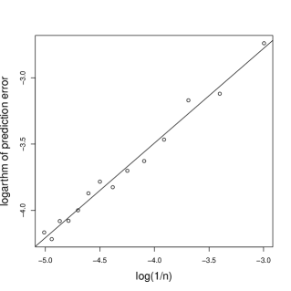
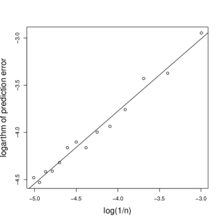
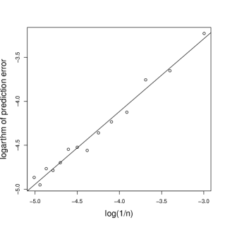
Figure 2: The regression line of $\log\mathcal{E}$ on $\log(1/n)$, under the four combinations of $(m_{0},m)$ in Table 2. Each point denotes one average prediction error for each $n$.

From Table 2, it can be seen that the estimated slopes are close to our theoretical assertions for these cases. Figure 2 shows the scattered points and the regression lines under the four combinations of $(m_{0},m)$ in Table 2. From the $R$-squared values and Figure 2, we can see that the regression lines fit the scattered points well.

7 Conclusions and discussion

In this work, we provide some upper and lower error bounds for Gaussian process regression under misspecified correlation functions, when the observations are corrupted by noise. We show that the optimal convergence rate of Gaussian process regression can be achieved by using an oversmoothed Matérn correlation function and a quasi-uniform sampling scheme. We also show that if the underlying truth is a deterministic function, the optimal convergence rate can still be achieved by kernel ridge regression if the kernel function is oversmoothed or not “too undersmoothed”. Despite the difference of model assumptions and approaches in the proofs, we find an interesting connection between the constructed convergence rates of Gaussian process regression and kernel ridge regression. This connection is aligned with the connection between Gaussian process and reproducing kernel Hilbert space. The finding of the connection could serve as a bridge between Bayesian learning and frequentist learning, and may inspire new advances in these two seemingly separate fields.

There are several remaining problems. First, when the underlying truth is a Gaussian process, we consider fixed designs, which are also considered in Tuo and Wang, (2020); Wang et al., (2020); Tuo et al., (2020). Whether the results hold for random sampling needs further study. Second, in addition to prediction, uncertainty quantification plays an important role in statistics. Since Gaussian process regression imposes a probabilistic structure on the underlying truth, it naturally induces an uncertainty quantification methodology via confidence interval. Uncertainty quantification under misspecification will be pursued in the future.

Appendix A Reproducing kernel Hilbert space, Sobolev space and kernel ridge regression

Reproducing kernel Hilbert space plays an important role in the study of kernel ridge regression and Gaussian process regression. Suppose $\Omega\subset\mathbb{R}^{d}$ satisfies Condition (C1). Assume that $K:\Omega\times\Omega\rightarrow\mathbb{R}$ is a symmetric positive definite kernel function. Define the linear space

$$F_{K}(\Omega)=\left\{\sum_{k=1}^{n}\beta_{k}K(\cdot,{x}_{k}):\beta_{k}\in\mathbb{R},{x}_{k}\in\Omega,n\in\mathbb{N}\right\},$$ (A.1)

and equip this space with the bilinear form

$$\left\langle\sum_{k=1}^{n}\beta_{k}K(\cdot,{x}_{k}),\sum_{j=1}^{m}\gamma_{j}K(\cdot,x^{\prime}_{j})\right\rangle_{K}:=\sum_{k=1}^{n}\sum_{j=1}^{m}\beta_{k}\gamma_{j}K({x}_{k},x^{\prime}_{j}).$$

Then the reproducing kernel Hilbert space $\mathcal{N}_{K}(\Omega)$ generated by the kernel function $K$ is defined as the closure of $F_{K}(\Omega)$ under the inner product $\langle\cdot,\cdot\rangle_{K}$, and the norm of $\mathcal{N}_{K}(\Omega)$ is $\|f\|_{\mathcal{N}_{K}(\Omega)}=\sqrt{\langle f,f\rangle_{\mathcal{N}_{K}(\Omega)}}$, where $\langle\cdot,\cdot\rangle_{\mathcal{N}_{K}(\Omega)}$ is induced by $\langle\cdot,\cdot\rangle_{K}$. The following theorem gives another characterization of the reproducing kernel Hilbert space when $K$ is defined by a stationary kernel function $\Psi$, via the Fourier transform. Note that a kernel function $\Psi$ is said to be stationary if the value $\Psi(x,x^{\prime})$ only depends on the difference $x-x^{\prime}$. Thus, we can write $\Psi(x-x^{\prime}):=\Psi(x,x^{\prime})$.

Theorem A.1 (Theorem 10.12 of Wendland, (2004)).

Let $\Psi$ be a positive definite kernel function which is stationary, continuous and integrable in $\mathbb{R}^{d}$. Define

$$\mathcal{G}:=\{f\in L_{2}(\mathbb{R}^{d})\cap C(\mathbb{R}^{d}):\mathcal{F}(f)/\sqrt{\mathcal{F}(\Psi)}\in L_{2}(\mathbb{R}^{d})\},$$

with the inner product

$$\langle f,g\rangle_{\mathcal{N}_{\Psi}(\mathbb{R}^{d})}=(2\pi)^{-d/2}\int_{\mathbb{R}^{d}}\frac{\mathcal{F}(f)(\omega)\overline{\mathcal{F}(g)(\omega)}}{\mathcal{F}(\Psi)(\omega)}d\omega.$$

Then $\mathcal{G}=\mathcal{N}_{\Psi}(\mathbb{R}^{d})$, and both inner products coincide.

For an integer $k$, the Sobolev norm for function $g$ on $\mathbb{R}^{d}$ is defined by

$$\|g\|^{2}_{H^{k}(\mathbb{R}^{d})}=\int_{\mathbb{R}^{d}}|\mathcal{F}(g)(\omega)|^{2}(1+\|\omega\|_{2}^{2})^{k}d\omega,$$

and the inner product of a Sobolev space $H^{k}(\mathbb{R}^{d})$ is defined by

$$\langle f,g\rangle_{H^{k}(\mathbb{R}^{d})}=\int_{\mathbb{R}^{d}}\mathcal{F}(f)(\omega)\overline{\mathcal{F}(g)(\omega)}(1+\|\omega\|_{2}^{2})^{k}d\omega.$$

This definition can be naturally extended to Sobolev spaces with non-integer orders, which are commonly known as the fractional Sobolev spaces, denoted by $H^{m}(\mathbb{R}^{d})$ with a non-integer $m$.

Remark 8.

In this work, we are only interested in Sobolev spaces with $m>d/2$ because these spaces contain only continuous function according to the Sobolev embedding theorem.

A Sobolev space can also be defined on $\Omega\subset\mathbb{R}^{d}$, denoted by $H^{m}(\Omega)$, with norm

$$\|f\|_{H^{m}(\Omega)}=\inf\{\|f_{e}\|_{H^{m}(\mathbb{R}^{d})}:f_{e}\in H^{m}(\mathbb{R}^{d}),f_{e}|_{\Omega}=f\},$$

where $f_{e}|_{\Omega}$ denotes the restriction of $f_{e}$ to $\Omega$. It can be shown that $H^{m_{0}}(\mathbb{R}^{d})$ coincides with the reproducing kernel Hilbert space $\mathcal{N}_{\Psi}(\mathbb{R}^{d})$ with equivalent norms, if $\Psi$ satisfies Condition (C2) (Wendland, (2004), Corollary 10.13). By the extension theorem (DeVore and Sharpley,, 1993), $\mathcal{N}_{\Psi}(\Omega)$ also coincides with $H^{m_{0}}(\Omega)$, and two norms are equivalent.

Given the observations $(x_{k},y_{k})$ with relationship (3.1), the kernel ridge regression reconstructs a function $f\in\mathcal{N}_{\Psi}(\Omega)$ by using

$$\widehat{f}=\operatorname*{argmin}_{g\in\mathcal{N}_{\Psi}(\Omega)}\bigg{(}\frac{1}{n}\sum_{k=1}^{n}(y_{k}-g(x_{k}))^{2}+\lambda\|g\|^{2}_{\mathcal{N}_{\Psi}(\Omega)}\bigg{)},$$ (A.2)

where $\lambda$ is a prespecified regularization parameter. Under certain conditions and if $\Psi$ satisfies Condition (C2), the optimal order of magnitude of $\lambda$ is known in the literature (van de Geer,, 2000), given by $\lambda=Cn^{-\frac{2m_{0}}{2m_{0}+d}},$ where $C$ can be any fixed positive constant. The optimal choice of $\lambda$ leads to the optimal convergence rate under $L_{2}$ metric, which is $n^{-\frac{m_{0}}{2m_{0}+d}}$ (Stone,, 1982).

Appendix B Notation

We use $\langle\cdot,\cdot\rangle_{n}$ to denote the empirical inner product, which is defined by

$$\langle f,g\rangle_{n}=\frac{1}{n}\sum_{k=1}^{n}f(x_{k})g(x_{k})$$

for two functions $f$ and $g$, and let $\|g\|_{n}^{2}=\langle g,g\rangle_{n}$ be the empirical norm of function $g$. In particular, let

$$\langle\epsilon,f\rangle_{n}=\frac{1}{n}\sum_{k=1}^{n}\epsilon_{k}f(x_{k}),$$

where $\epsilon=(\epsilon_{1},\ldots,\epsilon_{n})^{T}$. For two vectors $v$ and $w$, we use $\langle v,w\rangle=v^{T}w$ to denote the inner product.

For notational simplification, let $h_{n}=h_{X_{n},\Omega}$ and $q_{n}=q_{X_{n}}$ be the fill distance and separation radius of design $X_{n}$, respectively. For the ease of treatment, in the rest of Appendix, we assume the regularization parameter $\lambda_{m}\asymp n^{\alpha}$ for some $\alpha\in\mathbb{R}$. We use $tr(A)$ to denote the trace of a matrix $A$.

Appendix C Proof of Proposition 4.1

Without loss of generality, assume $\sigma=1$. Notice that for any $u=(u_{1},...,u_{n})^{T}\in\mathbb{R}^{n}$ and any constant $C_{1}$,

$$\Psi(x-x)-2\sum_{j=1}^{n}u_{j}\Psi(x-x_{j})+\sum_{k=1}^{n}\sum_{j=1}^{n}u_{k}u_{j}\Psi(x_{k}-x_{j})+C_{1}\|u\|_{2}^{2}\geq C_{1}\|u\|_{2}^{2},$$

because $\Psi$ is positive definite. Plugging $u=(R+C_{1}I_{n})^{-1}r(x)$, we have

$$C_{1}r(x)^{T}(R+C_{1}I_{n})^{-2}r(x)\leq\Psi(x-x)-r(x)^{T}(R+C_{1}I_{n})^{-1}r(x).$$ (C.1)

If $C\leq\mu=\sigma_{\epsilon}^{2}/\sigma^{2}$, then direct computation shows that

$$\mathbb{E}(\widehat{f}_{G}(x)-Z(x))^{2}$$

$$= \Psi(x-x)-2r(x)^{T}(R+CI_{n})^{-1}r(x)+r(x)^{T}(R+CI_{n})^{-1}(R+\mu I_{n})(R+CI_{n})^{-1}r(x)$$

$$= \Psi(x-x)-2r(x)^{T}(R+CI_{n})^{-1}r(x)+r(x)^{T}(R+CI_{n})^{-1}(R+CI_{n})(R+CI_{n})^{-1}r(x)$$

$$+(\mu-C)r(x)^{T}(R+CI_{n})^{-2}r(x)$$

$$= \Psi(x-x)-r(x)^{T}(R+CI_{n})^{-1}r(x)+(\mu-C)r(x)^{T}(R+CI_{n})^{-2}r(x)$$

$$\leq \bigg{(}1+\frac{\mu-C}{C}\bigg{)}(\Psi(x-x)-r(x)^{T}(R+CI_{n})^{-1}r(x))$$

$$\leq \frac{\mu}{C}(\Psi(x-x)-r(x)^{T}(R+\mu I_{n})^{-1}r(x)),$$ (C.2)

where the first inequality is because of (C.1), and the second inequality is because of $(R+\mu I_{n})^{-1}\preceq(R+CI_{n})^{-1}$.

If $C>\mu$, then we have

$$\mathbb{E}(\widehat{f}_{G}(x)-Z(x))^{2}$$

$$= \Psi(x-x)-2r(x)^{T}(R+CI_{n})^{-1}r(x)+r(x)^{T}(R+CI_{n})^{-1}(R+\mu I_{n})(R+CI_{n})^{-1}r(x)$$

$$\leq \Psi(x-x)-r(x)^{T}(R+CI_{n})^{-1}r(x),$$ (C.3)

where the first inequality is because of $R+\mu I_{n}\preceq R+CI_{n}$.

For any $u=(u_{1},\ldots,u_{n})^{T}$, the Fourier inversion theorem yields

$$\Psi(x-x)-2\sum_{j=1}^{n}u_{j}\Psi(x-x_{j})+\sum_{k=1}^{n}\sum_{j=1}^{n}u_{k}u_{j}\Psi(x_{k}-x_{j})+C\|u\|_{2}^{2}$$

$$= \frac{1}{(2\pi)^{d/2}}\int_{\mathbb{R}^{d}}\bigg{|}\sum_{j=1}^{n}u_{j}e^{i\langle x_{j},\omega\rangle}-e^{i\langle x,\omega\rangle}\bigg{|}^{2}\mathcal{F}(\Psi)(\omega)d\omega+C\|u\|_{2}^{2}$$

$$\leq \frac{C}{\mu}\bigg{(}\frac{1}{(2\pi)^{d/2}}\int_{\mathbb{R}^{d}}\bigg{|}\sum_{j=1}^{n}u_{j}e^{i\langle x_{j},\omega\rangle}-e^{i\langle x,\omega\rangle}\bigg{|}^{2}\mathcal{F}(\Psi)(\omega)d\omega+\mu\|u\|_{2}^{2}\bigg{)}.$$ (C.4)

Let $u^{(1)}=(u_{1}^{(1)},...,u_{n}^{(1)})^{T}=(R+\mu I_{n})^{-1}r(x)$. Because $u^{(2)}=(u_{1}^{(2)},...,u_{n}^{(2)})^{T}=(R+CI_{n})^{-1}r(x)$ is the solution to the optimization problem

$$\min_{u\in\mathbb{R}^{n}}\Psi(x-x)-2\sum_{j=1}^{n}u_{j}\Psi(x-x_{j})+\sum_{k=1}^{n}\sum_{j=1}^{n}u_{k}u_{j}\Psi(x_{k}-x_{j})+C\|u\|_{2}^{2},$$

we have

$$\Psi(x-x)-r(x)^{T}(R+CI_{n})^{-1}r(x)$$

$$= \Psi(x-x)-2\sum_{j=1}^{n}u_{j}^{(2)}\Psi(x-x_{j})+\sum_{k=1}^{n}\sum_{j=1}^{n}u_{k}^{(2)}u_{j}^{(2)}\Psi(x_{k}-x_{j})+C\|u^{(2)}\|_{2}^{2}$$

$$\leq \Psi(x-x)-2\sum_{j=1}^{n}u_{j}^{(1)}\Psi(x-x_{j})+\sum_{k=1}^{n}\sum_{j=1}^{n}u_{k}^{(1)}u_{j}^{(1)}\Psi(x_{k}-x_{j})+C\|u^{(1)}\|_{2}^{2}$$

$$\leq \frac{C}{\mu}\bigg{(}\frac{1}{(2\pi)^{d/2}}\int_{\mathbb{R}^{d}}\bigg{|}\sum_{j=1}^{n}u_{j}^{(1)}e^{i\langle x_{j},\omega\rangle}-e^{i\langle x,\omega\rangle}\bigg{|}^{2}\mathcal{F}(\Psi)(\omega)d\omega+\mu\|u^{(1)}\|_{2}^{2}\bigg{)}$$

$$= \frac{C}{\mu}(\Psi(x-x)-r(x)^{T}(R+\mu I_{n})^{-1}r(x)),$$ (C.5)

where the second inequality is by (C). Combining (C) and (C), we finish the proof.

Appendix D Proof of Proposition 4.2

Let $I(x)=\Psi(x-x)-r(x)^{T}(R+\mu_{1}I_{n})^{-1}r(x)$. Consider function $g(t)=\Psi(x-t)-r(x)^{T}(R+\mu_{1}I_{n})^{-1}r(t)$. It can be seen that

$$I(x)=g(x)\leq\|g\|_{L_{\infty}(\Omega)}.$$ (D.1)

Direct computation shows that

$$\|g\|_{\mathcal{N}_{\Psi}(\Omega)}^{2}= \Psi(x-x)-2r(x)^{T}(R+\mu_{1}I_{n})^{-1}r(x)+r(x)^{T}(R+\mu_{1}I_{n})^{-1}R(R+\mu_{1}I_{n})^{-1}r(x)$$

$$\leq \Psi(x-x)-r(x)^{T}(R+\mu_{1}I_{n})^{-1}r(x)=I(x).$$ (D.2)

By the Gagliardo–Nirenberg interpolation inequality for functions in Sobolev spaces (Leoni,, 2017; Brezis and Mironescu,, 2019), it can be seen that

$$\|g\|_{L_{\infty}(\Omega)}\lesssim\|g\|_{L_{2}(\Omega)}^{1-\frac{d}{2m}}\|g\|_{H^{m}(\Omega)}^{\frac{d}{2m}}\lesssim\|g\|_{L_{2}(\Omega)}^{1-\frac{d}{2m}}\|g\|_{\mathcal{N}_{\Psi}(\Omega)}^{\frac{d}{2m}}\lesssim\|g\|_{L_{2}(\Omega)}^{1-\frac{d}{2m}}I(x)^{\frac{d}{4m}}.$$ (D.3)

It remains to bound $\|g\|_{L_{2}(\Omega)}$. Let $f_{1}(t)=r(x)^{T}(R+\mu_{1}I_{n})^{-1}r(t)$. It can be seen from the representer theorem that

$$f_{1}=\operatorname*{argmin}_{h\in\mathcal{N}_{\Psi}(\Omega)}\|\Psi(x-\cdot)-h\|_{n}^{2}+\frac{\mu_{1}}{n}\|h\|^{2}_{\mathcal{N}_{\Psi}(\Omega)}.$$ (D.4)

By Lemma G.4,

$$\|g\|_{L_{2}(\Omega)}\lesssim h_{n}^{m_{0}}\|g\|_{H^{m_{0}}(\Omega)}+\|g\|_{n}\lesssim h_{n}^{m_{0}}\|g\|_{\mathcal{N}_{\Psi}(\Omega)}+\|g\|_{n}\lesssim h_{n}^{m}I(x)^{1/2}+\|g\|_{n},$$ (D.5)

where the second inequality is by the equivalence of $\|\cdot\|_{H^{m_{0}}(\Omega)}$ and $\|\cdot\|_{\mathcal{N}_{\Psi}(\Omega)}$, and the last inequality is by (D).

The empirical norm $\|g\|_{n}$ can be bounded by

$$\|g\|_{n}^{2}= \|\Psi(x-\cdot)-f_{1}\|_{n}^{2}$$

$$= \|\Psi(x-\cdot)-f_{1}\|_{n}^{2}+\frac{\mu_{1}}{n}\|f_{1}\|^{2}_{\mathcal{N}_{\Psi}(\Omega)}-\frac{\mu_{1}}{n}\|f_{1}\|^{2}_{\mathcal{N}_{\Psi}(\Omega)}$$

$$\leq \|\Psi(x-\cdot)-\Psi(x-\cdot)\|_{n}^{2}+\frac{\mu_{1}}{n}\|\Psi(x-\cdot)\|^{2}_{\mathcal{N}_{\Psi}(\Omega)}-\frac{\mu_{1}}{n}r(x)^{T}(R+\mu_{1}I_{n})^{-1}R(R+\mu_{1}I_{n})^{-1}r(x)$$

$$= \frac{\mu_{1}}{n}\Psi(x-x)-\frac{\mu_{1}}{n}r(x)^{T}(R+\mu_{1}I_{n})^{-1}(R+\mu_{1}I_{n})(R+\mu_{1}I_{n})^{-1}r(x)$$

$$+\frac{\mu_{1}^{2}}{n}r(x)^{T}(R+\mu_{1}I_{n})^{-2}r(x)$$

$$= \frac{\mu_{1}}{n}\bigg{(}\Psi(x-x)-r(x)^{T}(R+\mu_{1}I_{n})^{-1}r(x)+\mu_{1}r(x)^{T}(R+\mu_{1}I_{n})^{-2}r(x)\bigg{)},$$ (D.6)

where the first inequality is because $f_{1}$ is the solution to (D.4).

Notice that for any $u=(u_{1},...,u_{n})^{T}\in\mathbb{R}^{n}$,

$$\Psi(x-x)-2\sum_{j=1}^{n}u_{j}\Psi(x-x_{j})+\sum_{k=1}^{n}\sum_{j=1}^{n}u_{k}u_{j}\Psi(x_{k}-x_{j})+\mu_{1}\|u\|_{2}^{2}\geq\mu_{1}\|u\|_{2}^{2},$$

because $\Psi$ is positive definite. Plugging $u=(R+\mu_{1}I_{n})^{-1}r(x)$, we have

$$\mu_{1}r(x)^{T}(R+\mu_{1}I_{n})^{-2}r(x)\leq\Psi(x-x)-r(x)^{T}(R+\mu_{1}I_{n})^{-1}r(x).$$ (D.7)

Therefore, (D.7) and (D) imply that

$$\|g\|_{n}^{2}\leq \frac{2\mu_{1}}{n}\bigg{(}\Psi(x-x)-r(x)^{T}(R+\mu_{1}I_{n})^{-1}r(x)\bigg{)}=\frac{2\mu_{1}}{n}I(x).$$ (D.8)

By (D.1), (D.3), (D.5), and (D.8), we have

$$I(x)\lesssim (h_{n}^{m_{0}}I(x)^{1/2}+\|g\|_{n})^{1-\frac{d}{2m_{0}}}I(x)^{\frac{d}{4m_{0}}}$$

$$\lesssim \bigg{(}h_{n}^{m_{0}}I(x)^{1/2}+\frac{\mu_{1}^{1/2}}{n^{1/2}}I(x)^{1/2}\bigg{)}^{1-\frac{d}{2m_{0}}}I(x)^{\frac{d}{4m_{0}}}$$

$$\lesssim \bigg{(}h_{n}^{m_{0}}+\frac{\mu_{1}^{1/2}}{n^{1/2}}\bigg{)}^{1-\frac{d}{2m_{0}}}I(x)^{1/2}\lesssim\bigg{(}\frac{\mu_{1}}{n}\bigg{)}^{1/2-\frac{d}{4m_{0}}}I(x)^{1/2},$$ (D.9)

where the last inequality is because $\mu_{1}\gtrsim n^{1-2m_{0}/d}$. It can be seen that (D) implies

$$I(x)\leq\bigg{(}\frac{\mu_{1}}{n}\bigg{)}^{1-\frac{d}{2m_{0}}}.$$

This finishes the proof.

Appendix E Proof of Theorem 4.3

We first present several lemmas used in this proof. Lemma E.1 is Lemma 24 in Tuo and Wang, (2020). The proof of Lemma E.2 is provided in Appendix L.1.

Lemma E.1.

Suppose $\Omega$ satisfies Condition (C1). Let $G$ be a zero-mean Gaussian process on $\Omega$ with continuous sample paths almost surely and with a finite maximum pointwise variance $\sigma^{2}_{G}=\sup_{x\in\Omega}\mathbb{E}G(x)^{2}<\infty$. Then for all $u>0$ and $1\leq p<\infty$, we have

$$\mathbb{P}\left(\|G\|_{L_{p}(\Omega)}-\mathbb{E}\|G\|_{L_{p}(\Omega)}>u\right)\leq e^{-u^{2}/(2C_{p}\sigma^{2}_{G})},$$

$$\mathbb{P}\left(\|G\|_{L_{p}(\Omega)}-\mathbb{E}\|G\|_{L_{p}(\Omega)}<-u\right)\leq e^{-u^{2}/(2C_{p}\sigma^{2}_{G})},$$

with $C_{p}={\rm Vol}(\Omega)^{2/p}$. Here ${\rm Vol}(\Omega)$ denotes the volume of $\Omega$.

Lemma E.2.

Suppose the design points $X=\{x_{1},...,x_{n}\}$ and the separation radius of $X$ $q_{X}\lesssim 1$. Let $\Psi$ be a Matérn correlation function satisfying Condition (C2) and $\Lambda_{X}$ be the maximum eigenvalue of matrix $(\Psi(x_{j}-x_{k}))_{jk}$. Then

$$\Lambda_{X}\leq Cq_{X}^{-d},$$

where $C$ is a constant depending on $\Psi$ and $\Omega$.

Now we begin to prove Theorem 4.3. Recall that $y_{j}=Z(x_{j})+\epsilon_{j}$. Let $\epsilon=(\epsilon_{1},...,\epsilon_{n})^{T}$ and $F=(Z(x_{1}),...,Z(x_{n}))^{T}$. Therefore,

$$\widehat{f}_{G}(x)=r_{m}(x)^{T}(R_{m}+\mu_{m}I_{n})^{-1}F+r_{m}(x)^{T}(R_{m}+\mu_{m}I_{n})^{-1}\epsilon.$$

Direct computation shows that

$$(Z(x)-\widehat{f}_{G}(x))^{2}= (Z(x)-r_{m}(x)^{T}(R_{m}+\mu_{m}I_{n})^{-1}F-r_{m}(x)^{T}(R_{m}+\mu_{m}I_{n})^{-1}\epsilon)^{2}$$

$$\leq 2(Z(x)-r_{m}(x)^{T}(R_{m}+\mu_{m}I_{n})^{-1}F)^{2}+2(r_{m}(x)^{T}(R_{m}+\mu_{m}I_{n})^{-1}\epsilon)^{2}$$

$$= 2I_{1}(x)+2I_{2}(x),$$ (E.1)

where the inequality is by the Cauchy-Schwarz inequality. Let $G(x)=Z(x)-r_{m}(x)^{T}(R_{m}+\mu_{m}I_{n})^{-1}F$. It can be seen that $G$ is also a mean zero Gaussian process.

By Jensen’s inequality and Fubini’s theorem,

$$(\mathbb{E}\|G\|_{L_{2}(\Omega)})^{2}\leq\mathbb{E}\|G\|_{L_{2}(\Omega)}^{2}=\int_{\Omega}\mathbb{E}(Z(x)-r_{m}(x)^{T}(R_{m}+\mu_{m}I_{n})^{-1}F)^{2}dx$$

$$= \int_{\Omega}\mathbb{E}I_{1}(x)dx\leq{\rm Vol}(\Omega)\sup_{x\in\Omega}\mathbb{E}I_{1}(x),$$ (E.2)

where Vol$(\Omega)$ is the volumn of $\Omega$.

Next, we provide a uniform upper bound on $\mathbb{E}I_{1}(x)$. Direct computation gives us

$$\mathbb{E}I_{1}=\Psi(x-x)-2r_{m}(x)^{T}(R_{m}+\mu_{m}I_{n})^{-1}r(x)+r_{m}(x)^{T}(R_{m}+\mu_{m}I_{n})^{-1}R(R_{m}+\mu_{m}I_{n})^{-1}r_{m}(x),$$

where $r(x)$ and $R$ are as in (3.2).

By the Fourier inversion theorem, for $u=(u_{1},...,u_{n})^{T}=(R_{m}+\mu_{m}I_{n})^{-1}r_{m}(x)$, we have

$$\mathbb{E}I_{1}(x)=\int_{\mathbb{R}^{d}}\left|\sum_{j=1}^{n}u_{j}e^{-i\langle x_{j},\omega\rangle}-e^{-i\langle x,\omega\rangle}\right|^{2}\mathcal{F}(\Psi)(\omega)d\omega$$

$$= \int_{\|\omega\|_{2}\leq\gamma}\left|\sum_{j=1}^{n}u_{j}e^{-i\langle x_{j},\omega\rangle}-e^{-i\langle x,\omega\rangle}\right|^{2}\mathcal{F}(\Psi)(\omega)d\omega+\int_{\|\omega\|_{2}>\gamma}\left|\sum_{j=1}^{n}u_{j}e^{-i\langle x_{j},\omega\rangle}-e^{-i\langle x,\omega\rangle}\right|^{2}\mathcal{F}(\Psi)(\omega)d\omega$$

$$= I_{11}+I_{12},$$ (E.3)

where $\gamma>1$ will be determined later.

The first term $I_{11}$ can be bounded by

$$I_{11}\lesssim \int_{\|\omega\|_{2}\leq\gamma}\left|\sum_{j=1}^{n}u_{j}e^{-i\langle x_{j},\omega\rangle}-e^{-i\langle x,\omega\rangle}\right|^{2}(1+\|\omega\|_{2}^{2})^{-m_{0}}d\omega$$

$$\lesssim \gamma^{2m-2m_{0}}\int_{\|\omega\|_{2}\leq\gamma}\left|\sum_{j=1}^{n}u_{j}e^{-i\langle x_{j},\omega\rangle}-e^{-i\langle x,\omega\rangle}\right|^{2}(1+\|\omega\|_{2}^{2})^{-m}d\omega$$

$$\lesssim \gamma^{2m-2m_{0}}\int_{\|\omega\|_{2}\leq\gamma}\left|\sum_{j=1}^{n}u_{j}e^{-i\langle x_{j},\omega\rangle}-e^{-i\langle x,\omega\rangle}\right|^{2}\mathcal{F}(\Phi)(\omega)d\omega,$$ (E.4)

where the first and third inequalities are because of Conditions (C2) and (C3), respectively.

By the Cauchy-Schwarz inequality, the second term $I_{12}$ can be further split to

$$I_{12}\leq 2\int_{\|\omega\|_{2}>\gamma}\left|\sum_{j=1}^{n}u_{j}e^{-i\langle x_{j},\omega\rangle}\right|^{2}\mathcal{F}(\Psi)(\omega)d\omega+2\int_{\|\omega\|_{2}>\gamma}\left|e^{-i\langle x,\omega\rangle}\right|^{2}\mathcal{F}(\Psi)(\omega)d\omega$$

$$= I_{3}+I_{4}.$$ (E.5)

Since $\Psi$ satisfies Condition (C2), the term $I_{4}$ can be bounded by

$$I_{4}\lesssim\int_{\|\omega\|_{2}>\gamma}(1+\|\omega\|_{2}^{2})^{-m_{0}}d\omega\lesssim\gamma^{-2m_{0}+d},$$ (E.6)

and the term $I_{3}$ can be bounded by

$$I_{3} \lesssim\int_{\|\omega\|_{2}>\gamma}\left|\sum_{j=1}^{n}u_{j}e^{-i\langle x_{j},\omega\rangle}\right|^{2}(1+\|\omega\|_{2}^{2})^{-m_{0}}d\omega$$

$$\lesssim\gamma^{d}\int_{\|\omega\|_{2}>1}\left|\sum_{j=1}^{n}u_{j}e^{-i\gamma\langle x_{j},\omega\rangle}\right|^{2}(1+\gamma^{2}\|\omega\|_{2}^{2})^{-m_{0}}d\omega$$

$$\lesssim\gamma^{d-2m_{0}}\int_{\|\omega\|_{2}>1}\left|\sum_{j=1}^{n}u_{j}e^{-i\gamma\langle x_{j},\omega\rangle}\right|^{2}(1+\|\omega\|_{2}^{2})^{-m_{0}}d\omega$$

$$\lesssim\gamma^{d-2m_{0}}\int_{\mathbb{R}^{d}}\left|\sum_{j=1}^{n}u_{j}e^{-i\gamma\langle x_{j},\omega\rangle}\right|^{2}(1+\|\omega\|_{2}^{2})^{-m_{0}}d\omega,$$ (E.7)

where the second inequality is by the change of variables, and the third inequality is by the fact that $(1+\gamma^{2}\|\omega\|_{2}^{2})^{-m_{0}}\leq(\gamma^{2}(1+\|\omega\|_{2}^{2})/2)^{-m_{0}}$ for $\|\omega\|_{2}\geq 1$.

Putting (E.6) and (E) into (E), we obtain

$$I_{12} \lesssim\gamma^{d-2m_{0}}\int_{\mathbb{R}^{d}}\left|\sum_{j=1}^{n}u_{j}e^{-i\gamma\langle x_{j},\omega\rangle}\right|^{2}(1+\|\omega\|_{2}^{2})^{-m_{0}}d\omega+\gamma^{-2m_{0}+d}$$

$$\lesssim\gamma^{d-2m_{0}}\int_{\mathbb{R}^{d}}\left|\sum_{j=1}^{n}u_{j}e^{-i\gamma\langle x_{j},\omega\rangle}\right|^{2}\mathcal{F}(\Psi)(\omega)d\omega+\gamma^{-2m_{0}+d}$$

$$=\gamma^{d-2m_{0}}\sum_{j,k=1}^{n}u_{j}u_{k}\Psi(\gamma x_{j}-\gamma x_{k})+\gamma^{-2m_{0}+d}$$

$$\leq\gamma^{d-2m_{0}}\Lambda_{\gamma X}\|u\|_{2}^{2}+\gamma^{-2m_{0}+d},$$ (E.8)

where the second inequality is because $\Psi$ satisfies Condition (C2), and $\gamma X=\{\gamma x_{1},...,\gamma x_{n}\}$. The separation distance of $\gamma X$ is $\gamma q_{X}$, which, together with Lemma E.2, implies $\Lambda_{\gamma X}\leq C(\gamma q_{X})^{-d}$ (it can be seen by the choice of $\gamma$ later, $\gamma q_{X}\lesssim 1$). Plugging (E) and (E) into (E), we have

$$\mathbb{E}I_{1}(x)$$

$$\lesssim \gamma^{2m-2m_{0}}\int_{\|\omega\|_{2}\leq\gamma}\left|\sum_{j=1}^{n}u_{j}e^{-i\langle x_{j},\omega\rangle}-e^{-i\langle x,\omega\rangle}\right|^{2}\mathcal{F}(\Phi)(\omega)d\omega+\gamma^{d-2m_{0}}\Lambda_{\gamma X}\|u\|_{2}^{2}+\gamma^{-2m_{0}+d}$$

$$\lesssim \gamma^{2m-2m_{0}}\int_{\|\omega\|_{2}\leq\gamma}\left|\sum_{j=1}^{n}u_{j}e^{-i\langle x_{j},\omega\rangle}-e^{-i\langle x,\omega\rangle}\right|^{2}\mathcal{F}(\Phi)(\omega)d\omega+\gamma^{d-2m_{0}}(\gamma q_{X})^{-d}\|u\|_{2}^{2}+\gamma^{-2m_{0}+d}$$

$$\lesssim \gamma^{2m-2m_{0}}\bigg{(}\int_{\|\omega\|_{2}\leq\gamma}\left|\sum_{j=1}^{n}u_{j}e^{-i\langle x_{j},\omega\rangle}-e^{-i\langle x,\omega\rangle}\right|^{2}\mathcal{F}(\Phi)(\omega)d\omega+\gamma^{-2m}(q_{X})^{-d}\|u\|_{2}^{2}\bigg{)}+\gamma^{-2m_{0}+d}.$$ (E.9)

Take $\gamma=\mu_{m}^{-\frac{1}{2m}}(q_{X})^{-d/2m}$ such that $\gamma^{-2m}(q_{X})^{-d}=\mu_{m}$. Clearly, $\gamma q_{X}\lesssim 1$. By (E), $\mathbb{E}I_{1}(x)$ can be further bounded by

$$\mathbb{E}I_{1}(x)\lesssim \mu_{m}^{-\frac{m-m_{0}}{m}}q_{X}^{-\frac{(m-m_{0})d}{m}}\bigg{(}\int_{\|\omega\|_{2}\leq\gamma}\left|\sum_{j=1}^{n}u_{j}e^{-i\langle x_{j},\omega\rangle}-e^{-i\langle x,\omega\rangle}\right|^{2}\mathcal{F}(\Phi)(\omega)d\omega+\mu_{m}\|u\|_{2}^{2}\bigg{)}$$

$$+\mu_{m}^{\frac{2m_{0}-d}{2m}}(q_{X})^{\frac{(2m_{0}-d)d}{2m}}$$

$$\lesssim \mu_{m}^{-\frac{m-m_{0}}{m}}q_{X}^{-\frac{(m-m_{0})d}{m}}\bigg{(}\int_{\mathbb{R}^{d}}\left|\sum_{j=1}^{n}u_{j}e^{-i\langle x_{j},\omega\rangle}-e^{-i\langle x,\omega\rangle}\right|^{2}\mathcal{F}(\Phi)(\omega)d\omega+\mu_{m}\|u\|_{2}^{2}\bigg{)}$$

$$+\mu_{m}^{\frac{2m_{0}-d}{2m}}(q_{X})^{\frac{(2m_{0}-d)d}{2m}}$$

$$= \mu_{m}^{-\frac{m-m_{0}}{m}}q_{X}^{-\frac{(m-m_{0})d}{m}}\bigg{(}\Phi(x-x)-2\sum_{j=1}^{n}u_{j}\Phi(x-x_{j})+\sum_{j,k=1}^{n}u_{j}u_{k}\Phi(x_{j}-x_{k})+\mu_{m}\|u\|_{2}^{2}\bigg{)}$$

$$+\mu_{m}^{\frac{2m_{0}-d}{2m}}(q_{X})^{\frac{(2m_{0}-d)d}{2m}}$$

$$= \mu_{m}^{-\frac{m-m_{0}}{m}}q_{X}^{-\frac{(m-m_{0})d}{m}}(\Phi(x-x)-r_{m}(x)^{T}(R_{m}+\mu_{m}I_{n})^{-1}r_{m}(x))+\mu_{m}^{\frac{2m_{0}-d}{2m}}(q_{X})^{\frac{(2m_{0}-d)d}{2m}}$$

$$\lesssim \mu_{m}^{-\frac{m-m_{0}}{m}}q_{X}^{-\frac{(m-m_{0})d}{m}}(\mu_{m}/n)^{1-\frac{d}{2m}}+\mu_{m}^{\frac{2m_{0}-d}{2m}}(q_{X})^{\frac{(2m_{0}-d)d}{2m}},$$ (E.10)

where the last inequality is by applying Proposition 4.2 to the correlation function $\Phi$.

Let $T=\mu_{m}^{-\frac{m-m_{0}}{m}}q_{X}^{-\frac{(m-m_{0})d}{m}}(\mu_{m}/n)^{1-\frac{d}{2m}}+\mu_{m}^{\frac{2m_{0}-d}{2m}}(q_{X})^{\frac{(2m_{0}-d)d}{2m}}$. Lemma E.1, (E), and (E) imply that for all $t_{1}>0$, with probability at least $1-\exp(-Ct_{1}^{2})$,

$$\|G\|_{L_{2}(\Omega)}\lesssim(1+t_{1})T^{1/2}.$$

which implies

$$\|G\|_{L_{2}(\Omega)}^{2}\lesssim(1+t_{1})^{2}T.$$ (E.11)

Next, we consider $I_{2}(x)$. This can be done by applying Theorem I.1. Recall that $I_{2}(x)=(r_{m}(x)^{T}(R_{m}+\mu_{m}I_{n})^{-1}\epsilon)^{2}$. Define $f_{2}(x)=0$ for all $x\in\Omega$, i.e., $f_{2}$ is a zero function. Clearly, $f_{2}\in\mathcal{N}_{\Phi}(\Omega)$ with $\|f_{2}\|_{\mathcal{N}_{\Phi}(\Omega)}=0$. Let $\widehat{f}_{2}(x)=r_{m}(x)^{T}(R_{m}+\mu_{m}I_{n})^{-1}\epsilon$, then $\|\widehat{f}_{2}\|_{L_{2}(\Omega)}^{2}=\int_{x\in\Omega}I_{2}(x)dx$. By the representer theorem, $\widehat{f}_{2}$ is the solution to

$$\min_{\widehat{g}\in\mathcal{N}_{\Phi}(\Omega)}\frac{1}{n}\sum_{j=1}^{n}\left(\widehat{g}(x_{j})-\epsilon_{j}\right)^{2}+\frac{\mu_{m}}{n}\|\widehat{g}\|_{\mathcal{N}_{\Phi}(\Omega)}.$$

Theorem I.1 tells us that for all $t>C_{0}$ (with appropriate changes of notation), with probability at least $1-C_{1}\exp(-C_{2}t^{2})$,

$$\|f_{2}-\widehat{f}_{2}\|_{L_{2}(\Omega)}^{2}\leq C_{3}t^{2}n^{-1}(\mu_{m}/n)^{-\frac{d}{2m}},$$

which implies

$$\int_{x\in\Omega}I_{2}(x)dx=\|\widehat{f}_{2}\|_{L_{2}(\Omega)}^{2}\leq C_{3}t^{2}n^{-1}(\mu_{m}/n)^{-\frac{d}{2m}}$$ (E.12)

since $f_{2}=0$. Note that (E) implies $\|Z-\widehat{f}_{G}\|_{L_{2}(\Omega)}^{2}\lesssim\|G\|_{L_{2}(\Omega)}^{2}+\|\widehat{f}_{2}\|_{L_{2}(\Omega)}^{2}$. Thus, by (E.11) and (E.12), we finish the proof of Theorem 4.3.

Appendix F Proof of Theorem 4.5

Note that $y_{j}=Z(x_{j})+\epsilon_{j}$. Let $\epsilon=(\epsilon_{1},...,\epsilon_{n})^{T}$ and $F=(Z(x_{1}),...,Z(x_{n}))^{T}$. Therefore,

$$\widehat{f}_{G}(x)=r_{m}(x)^{T}(R_{m}+\mu_{m}I_{n})^{-1}F+r_{m}(x)^{T}(R_{m}+\mu_{m}I_{n})^{-1}\epsilon.$$

Similar to (E), we have

$$(Z(x)-\widehat{f}_{G}(x))^{2}\leq 2(Z(x)-r_{m}(x)^{T}(R_{m}+\mu_{m}I_{n})^{-1}F)^{2}+2(r_{m}(x)^{T}(R_{m}+\mu_{m}I_{n})^{-1}\epsilon)^{2}$$

$$= 2I_{1}(x)+2I_{2}(x).$$

Let $G(x)=Z(x)-r_{m}(x)^{T}(R_{m}+\mu_{m}I_{n})^{-1}F$, which is also a mean zero Gaussian process.

Similar to (E), we can obtain that

$$(\mathbb{E}\|G\|_{L_{2}(\Omega)})^{2}\leq{\rm Vol}(\Omega)\sup_{x\in\Omega}\mathbb{E}I_{1}(x).$$ (F.1)

Direct computation gives us

$$\mathbb{E}I_{1}(x)=\Psi(x-x)-2r_{m}(x)^{T}(R_{m}+\mu_{m}I_{n})^{-1}r(x)+r_{m}(x)^{T}(R_{m}+\mu_{m}I_{n})^{-1}R(R_{m}+\mu_{m}I_{n})^{-1}r_{m}(x).$$

By the Fourier inversion theorem and Conditions (C2) and (C3), for $u=(u_{1},...,u_{n})^{T}=(R_{m}+\mu_{m}I_{n})^{-1}r_{m}(x)$, we have

$$\mathbb{E}I_{1}(x)= \int_{\mathbb{R}^{d}}\left|\sum_{j=1}^{n}u_{j}e^{-i\langle x_{j},\omega\rangle}-e^{-i\langle x,\omega\rangle}\right|^{2}\mathcal{F}(\Psi)(\omega)d\omega$$

$$\leq C_{1}\int_{\mathbb{R}^{d}}\left|\sum_{j=1}^{n}u_{j}e^{-i\langle x_{j},\omega\rangle}-e^{-i\langle x,\omega\rangle}\right|^{2}(1+\|\omega\|_{2}^{2})^{-m_{0}}d\omega$$

$$\leq C_{1}\int_{\mathbb{R}^{d}}\left|\sum_{j=1}^{n}u_{j}e^{-i\langle x_{j},\omega\rangle}-e^{-i\langle x,\omega\rangle}\right|^{2}(1+\|\omega\|_{2}^{2})^{-m}d\omega$$

$$\leq C_{2}\int_{\mathbb{R}^{d}}\left|\sum_{j=1}^{n}u_{j}e^{-i\langle x_{j},\omega\rangle}-e^{-i\langle x,\omega\rangle}\right|^{2}\mathcal{F}(\Phi)(\omega)d\omega$$

$$= C_{2}(\Phi(x-x)-r_{m}(x)^{T}(R_{m}+\mu_{m}I_{n})^{-1}r_{m}(x))=:I_{3}(x),$$ (F.2)

where the second inequality is because $m\leq m_{0}$.

Applying Proposition 4.2 to the correlation function $\Phi$ implies that

$$I_{3}(x)\leq C_{3}(\mu_{m}/n)^{1-\frac{d}{2m}}.$$ (F.3)

Lemma E.1, (F.1), (F), and (F.3) imply that for all $t_{1}>0$, with probability at least $1-\exp(-Ct_{1}^{2})$,

$$\|G\|_{L_{2}(\Omega)}^{2}\leq C_{4}(1+t_{1})^{2}(\mu_{m}/n)^{1-\frac{d}{2m}}.$$ (F.4)

Similar to the proof of (E.12), for all $t_{2}\geq C_{0}$, with probability at least $1-\exp(-t_{2}^{2})$,

$$\int_{x\in\Omega}I_{2}(x)dx\leq C_{5}t_{2}^{2}\mu_{m}^{-\frac{d}{2m}}n^{-\left(1-\frac{d}{2m}\right)}.$$ (F.5)

By the fact $\|Z-\widehat{f}_{G}\|_{L_{2}(\Omega)}^{2}\lesssim\|G\|_{L_{2}(\Omega)}^{2}+\|\widehat{r}_{m}(x)^{T}(R_{m}+\mu_{m}I_{n})^{-1}\epsilon\|_{L_{2}(\Omega)}^{2}$, (F.4), and (F.5), we finish the proof of Theorem 4.5.

Appendix G Proof of Theorem 4.7

We first present several lemmas. Lemma G.1 is Lemma F.7 of Wang, (2020).

Lemma G.1.

Suppose $A,B$ and $C\in\mathbb{R}^{n\times n}$ are positive definite matrices. We have

$$\text{tr}((A+B)(A+B+C)^{-1})\geq\text{tr}(A(A+C)^{-1}),$$

and $$\text{tr}((A+B)^{2}(A+B+C)^{-2})\geq\text{tr}(A^{2}(A+C)^{-2}).$$

Let $K$ be a stationary correlation function. Since a correlation function is positive definite, by Mercer’s theorem, there exists a countable set of positive eigenvalues $\lambda_{1}\geq\lambda_{2}\geq...>0$ and an orthonormal basis for $L_{2}(\Omega)$ $\{\varphi_{k}\}_{k\in\mathbb{N}}$ such that

$$K(x-y)=\sum_{k=1}^{\infty}\lambda_{k}\varphi_{k}(x)\varphi_{k}(y),\quad x,y\in\Omega,$$ (G.1)

where the summation is uniformly and absolutely convergent.

Lemma G.2 states the asymptotic rate of the eigenvalues of $K$, which is implied by the proof of Lemma 18 of Tuo and Wang, (2020).

Lemma G.2.

Suppose Condition (C1) holds. Suppose $K$ is a stationary correlation function satisfying Condition (C2) and has an expansion as in (G.1). Then, $\lambda_{k}\asymp k^{-2m_{0}/d}$.

We need the following technical assumption.

Assumption G.0.1.

Suppose there exists a stationary correlation function $K$ satisfying Condition (C2) and a constant $A_{0}>0$ such that

$$\left\|\frac{\mathcal{F}(K)}{\mathcal{F}(\Psi)}\right\|_{L_{\infty}(\mathbb{R}^{d})}\leq A_{0},$$ (G.2)

and $K$ has an expansion as in (G.1) with eigenfunctions $\|\varphi_{k}\|_{L_{\infty}(\Omega)}\leq C$ for all $k=1,2,...$, where $C>0$ not depending on $k$.

Lemma G.3 states that the MSPE $\mathbb{E}(Z(x)-\widehat{f}_{G}(x))^{2}$ can be further bounded by the term related to $K$, and the proof is in Appendix L.2.

Lemma G.3.

Let $\Psi$ be a correlation function satisfying Condition (C2), and $Z\sim GP(0,\sigma^{2}\Psi)$. Assume Assumption G.0.1 holds. Let $\{x_{1},...,x_{n}\}$ be a set of design points. Then for all $x\in\Omega$,

$${\rm Var}[Z(x)|Y]\gtrsim K(x-x)-r_{K}(x)^{T}(R_{K}+\mu I_{n})^{-1}r_{K}(x),$$

where $R_{K}=(K(x_{j}-x_{k}))_{jk}$, $r_{K}(x)=(K(x-x_{1}),...,K(x-x_{n}))^{T}$, and $Y$ and $\mu$ are as in (3.2).

Lemma G.4 and Lemma G.5 state that under fixed designs, the empirical norm is close to the $L_{2}$ norm. Lemma G.4 can be found in Madych and Potter, (1985); Rieger, (2008). The proof of Lemma G.5 is merely repeating the process of proving Lemma G.4 as in Madych and Potter, (1985), thus is omitted.

Lemma G.4.

Suppose $g\in H^{m}(\Omega)$ for some $m>d/2$. Suppose Condition (C4) holds. Then we have

$$\|g\|_{L_{2}(\Omega)}\leq C(h_{n}^{m}\|g\|_{H^{m}(\Omega)}+\|g\|_{n})$$

holds for all $n$, where $C$ is a positive constant not depending on $g$ and $n$.

Remark 9.

Lemma G.4 is a stronger version of Lemma 3.4 in Utreras, (1988). In Lemma 3.4 of Utreras, (1988), the fixed designs are assumed to be quasi-uniform. Lemma 3.4 of Utreras, (1988) is used in Tuo et al., (2020).

Lemma G.5.

Suppose $g\in H^{m}(\Omega)$ for some $m>d/2$. Suppose Condition (C4) holds. Then we have

$$\|g\|_{n}\leq C(h_{n}^{m}\|g\|_{H^{m}(\Omega)}+\|g\|_{L_{2}(\Omega)})$$

holds for all $n$, where $C$ is a positive constant not depending on $g$ and $n$.

By Lemma G.3, it suffices to show

$$\int_{x\in\Omega}K(x-x)-r_{K}(x)^{T}(R_{K}+\mu I_{n})^{-1}r_{K}(x)dx\gtrsim n^{-\frac{2m_{0}-d}{2m_{0}}},$$

where $K,r_{K},R_{K},\mu$ are as in Lemma G.3. This is because for any linear predictor $\widehat{f}_{G}$,

$$\mathbb{E}(Z(x)-\widehat{f}_{G}(x))^{2}\geq{\rm Var}[Z(x)|Y],\forall x\in\Omega.$$

Notice that for any $u=(u_{1},...,u_{n})^{T}\in\mathbb{R}^{n}$,

$$K(x-x)-2\sum_{j=1}^{n}u_{j}K(x-x_{j})+\sum_{k=1}^{n}\sum_{j=1}^{n}u_{k}u_{j}K(x_{k}-x_{j})+\mu\|u\|_{2}^{2}\geq\mu\|u\|_{2}^{2},$$ (G.3)

since $K$ is positive definite. Let $u(x)=(u_{1}(x),...,u_{n}(x))^{T}=(R_{K}+\mu I_{n})^{-1}r_{K}(x)$, (G.3) implies

$$\mu r_{K}(x)^{T}(R_{K}+\mu I_{n})^{-2}r_{K}(x)\leq K(x-x)-r_{K}(x)^{T}(R_{K}+\mu I_{n})^{-1}r_{K}(x).$$ (G.4)

From (G.4), it can be seen that it is sufficient to provide a lower bound on $I(x):=r_{K}(x)^{T}(R_{K}+\mu I_{n})^{-2}r_{K}(x)$, because $\mu$ is a constant.

Let $p=\lfloor n^{d/(2m_{0})}\rfloor$, where $\lfloor\cdot\rfloor$ is the floor function. Let $K_{1}=\frac{1}{\sqrt{n}}(\varphi_{1}(X),...,\varphi_{p}(X))$, and $K_{2}=\frac{1}{\sqrt{n}}(\varphi_{p+1}(X),\varphi_{p+2}(X),...)$, where $\varphi_{k}(X)=(\varphi_{k}(x_{1}),...,\varphi_{k}(x_{n}))^{T}$ for $k=1,2,...$, and $\varphi_{k}$’s are as in (G.1). Let $\Lambda_{1}=\mbox{diag}(n\lambda_{1},...,n\lambda_{p})$ and $\Lambda_{2}=\mbox{diag}(n\lambda_{p+1},...)$, where $\lambda_{k}$’s are as in (G.1). Therefore, $R_{K}=\sum_{k=1}^{\infty}\lambda_{k}\varphi_{k}(X)\varphi_{k}(X)^{T}=K_{1}\Lambda_{1}K_{1}^{T}+K_{2}\Lambda_{2}K_{2}^{T}$. Note that for any functions $v_{1},v_{2}\in H^{m_{0}}(\Omega)$, $\|v_{1}v_{2}\|_{H^{m_{0}}(\Omega)}\leq C\|v_{1}\|_{H^{m_{0}}(\Omega)}\|v_{2}\|_{H^{m_{0}}(\Omega)}$ (Adams and Fournier,, 2003). Because $I(x)=u(x)^{T}u(x)$, we have

$$\|I\|_{H^{m_{0}}(\Omega)}=\left\|\sum_{k=1}^{n}u_{k}^{2}\right\|_{H^{m_{0}}(\Omega)}\leq C\sum_{k=1}^{n}\|u_{k}\|_{H^{m_{0}}(\Omega)}^{2}\leq C_{1}\sum_{k=1}^{n}\|u_{k}\|_{\mathcal{N}_{K}(\Omega)}^{2}$$

$$= C_{1}\sum_{k=1}^{n}((R_{K}+\mu I_{n})^{-1})_{k}^{T}R_{K}((R_{K}+\mu I_{n})^{-1})_{k}=C_{1}{\rm tr}((R_{K}+\mu I_{n})^{-2}R_{K}),$$ (G.5)

where the first inequality is by the triangle inequality, and $((R_{K}+\mu I_{n})^{-1})_{k}$ denotes the $k$-th row of $(R_{K}+\mu I_{n})^{-1}$.

Next we provide a lower bound on $\lambda_{\min}(K_{1}^{T}K_{1})$ and an upper bound on tr$(K_{2}^{T}\Lambda_{2}K_{2})$. For any $a=(a_{1},...,a_{p})^{T}\in\mathbb{R}^{p}$ such that $\|a\|_{2}=1$, consider function $g_{1}=\sum_{k=1}^{p}a_{k}\varphi_{k}$. Since $\varphi_{i}$’s are orthonormal, $\|g\|_{L_{2}(\Omega)}=1$. By Lemma G.2, $\|g_{1}\|^{2}_{H^{m_{0}}(\Omega)}\leq C_{1}\|g_{1}\|^{2}_{\mathcal{N}_{K}(\Omega)}\leq C_{1}\|\varphi_{p}\|^{2}_{\mathcal{N}_{K}(\Omega)}\leq C_{2}/\lambda_{p}\leq C_{3}p^{2m_{0}/d}\leq C_{3}n$. Therefore, by Lemma G.4 and Condition (C4),

$$\|g\|_{L_{2}(\Omega)}\leq C_{4}(h_{n}^{m_{0}}\|g_{1}\|_{H^{m_{0}}(\Omega)}+\|g\|_{n})$$

$$\leq C_{5}(n^{-m_{0}/d}n^{1/2}+\|g\|_{n})$$

which implies

$$\|g\|_{n}\geq\frac{1}{C_{5}}\|g\|_{L_{2}(\Omega)}-n^{(d-2m_{0})/2d}\geq\frac{1}{2C_{5}},$$

for some $n>N_{0}$, since $m_{0}>d/2$ and $n^{(d-2m_{0})/2d}$ converges to zero. Then we have

$$\lambda_{\min}(K_{1}^{T}K_{1})=\inf_{a\in\mathbb{R}^{p}}\|g\|_{n}^{2}\geq C_{6},$$ (G.6)

for some constant $C_{6}>0$.

Considering ${\rm tr}(K_{2}^{T}\Lambda_{2}K_{2})$, we have

$${\rm tr}(K_{2}^{T}\Lambda_{2}K_{2})=\sum_{k=p+1}^{\infty}\lambda_{k}\left(\sum_{j=1}^{n}\varphi_{k}(x_{j})^{2}\right)\leq nC_{7}^{2}\sum_{k=p+1}^{\infty}\lambda_{k}\leq C_{8}np^{-\frac{2m_{0}}{d}+1}\leq C_{8}n^{\frac{d}{2m_{0}}},$$ (G.7)

where the first inequality is by Assumption G.0.1, and the second inequality is by Lemma G.2 and the basic inequality $\sum_{k=m}^{\infty}k^{-2m_{0}/d}\lesssim m^{-2m_{0}/d+1}$.

By (G), $\|I\|_{H^{m_{0}}(\Omega)}$ can be further bounded by

$$\|I\|_{H^{m_{0}}(\Omega)}\leq C_{1}{\rm tr}((K_{1}\Lambda_{1}K_{1}^{T}+K_{2}\Lambda_{2}K_{2}^{T}+\mu I_{n})^{-2}(K_{1}\Lambda_{1}K_{1}^{T}+K_{2}\Lambda_{2}K_{2}^{T}))$$

$$\leq C_{1}({\rm tr}((K_{1}\Lambda_{1}K_{1}^{T}+\mu I_{n})^{-2}K_{1}\Lambda_{1}K_{1}^{T}))+C_{1}\mu^{-2}{\rm tr}(K_{2}\Lambda_{2}K_{2}^{T}).$$ (G.8)

Let $I_{1}={\rm tr}((K_{1}\Lambda_{1}K_{1}^{T}+\mu I_{n})^{-2}K_{1}\Lambda_{1}K_{1}^{T})$. We have

$$I_{1}= \sum_{i=1}^{p}\frac{\lambda_{i}(K_{1}\Lambda_{1}K_{1}^{T})}{(\lambda_{i}(K_{1}\Lambda_{1}K_{1}^{T})+\mu)^{2}}\leq\mu^{-2}p\leq\mu^{-2}n^{\frac{d}{2m_{0}}},$$ (G.9)

where $\lambda_{i}(K_{1}\Lambda_{1}K_{1}^{T})$ denote the $i$-th eigenvalue of $K_{1}\Lambda_{1}K_{1}^{T}$.

Combining (G.7), (G), and (G.9), we find that $\|I\|_{H^{m_{0}}(\Omega)}\leq C_{9}n^{\frac{d}{2m_{0}}}$.

Together with Lemma G.5, we have

$$\|I\|_{n}\leq C_{10}(h_{n}^{m_{0}}\|I\|_{H^{m_{0}}(\Omega)}+\|I\|_{L_{2}(\Omega)})\leq C_{11}(n^{\frac{d}{2m_{0}}-\frac{m_{0}}{d}}+\|I\|_{L_{2}(\Omega)}).$$ (G.10)

Let $I_{n}=\text{tr}(R_{K}^{2}(R_{K}+\mu I_{n})^{-2})$. Note that $\lambda_{i}(K_{1}\Lambda_{1}K_{1}^{T})=\lambda_{i}(K_{1}^{T}K_{1}\Lambda_{1})$ for $i=1,...,p$, because if $v_{i}$ is eigenvector corresponding to $i$-th eigenvalue of $K_{1}\Lambda_{1}K_{1}^{T}$, then

$$K_{1}\Lambda_{1}K_{1}^{T}v_{i}=\lambda_{i}v_{i}\Rightarrow K_{1}^{T}K_{1}\Lambda_{1}K_{1}^{T}v_{i}=\lambda_{i}K_{1}^{T}v_{i}.$$

By Lemma G.1 and $R_{K}=K_{1}\Lambda_{1}K_{1}^{T}+K_{2}\Lambda_{2}K_{2}^{T}$, it can be shown that

$$I_{n}\geq \text{tr}((K_{1}\Lambda_{1}K_{1}^{T})^{2}(K_{1}\Lambda_{1}K_{1}^{T}+\mu I)^{-2})$$

$$= \sum_{i=1}^{p}\bigg{(}\frac{\lambda_{i}(K_{1}\Lambda_{1}K_{1}^{T})}{\lambda_{i}(K_{1}\Lambda_{1}K_{1}^{T})+\mu}\bigg{)}^{2}$$

$$= \sum_{i=1}^{p}\bigg{(}\frac{\lambda_{i}(\Lambda_{1}K_{1}^{T}K_{1})}{\lambda_{i}(\Lambda_{1}K_{1}^{T}K_{1})+\mu}\bigg{)}^{2},$$

which implies

$$I_{n}\geq \text{tr}((\Lambda_{1}K_{1}^{T}K_{1})^{2}(\Lambda_{1}K_{1}^{T}K_{1}+\mu I)^{-2})\geq\text{tr}(\Lambda_{1}^{2}(\Lambda_{1}+\mu(K_{1}^{T}K_{1})^{-1})^{-2}).$$ (G.11)

Combining (G.6) with (G.11), we conclude that

$$I_{n}\geq\text{tr}(\Lambda_{1}^{2}(\Lambda_{1}+C_{12}I_{p})^{-2})\geq\sum_{k=1}^{p}\frac{\lambda_{k}^{2}}{(\lambda_{k}+C_{12}/n)^{2}}\geq C_{13}p\geq C_{14}n^{d/(2m_{0})},$$ (G.12)

where the third inequality is by Lemma G.2. It follows the Cauchy-Schwarz inequality that

$$\|I\|_{n}=\sqrt{\frac{1}{n}\sum_{k=1}^{n}(u(x_{k})^{T}u(x_{k}))^{2}}\geq\frac{1}{n}\sum_{k=1}^{n}u(x_{k})^{T}u(x_{k})=I_{n}/n\geq C_{14}n^{d/(2m_{0})-1}.$$

By (G.10), we have

$$\|I\|_{L_{2}(\Omega)}\geq\frac{1}{C_{10}}\|I\|_{n}-n^{d/(2m_{0})-\frac{m_{0}}{d}}\geq C_{15}n^{d/(2m_{0})-1}-n^{d/(2m_{0})-\frac{m_{0}}{d}}\gtrsim n^{d/(2m_{0})-1},$$

for some $n>N_{1}$ such that $C_{15}n^{d/(2m_{0})-1}>2n^{d/(2m_{0})-\frac{m_{0}}{d}}$, which can be done since $m_{0}>d$. Thus, for $n>\max(N_{0},N_{1})$, we have $\mathbb{E}\|Z-\widehat{f}_{G}\|_{L_{2}(\Omega)}^{2}\gtrsim n^{d/(2m_{0})-1}$. But for $n\leq\max(N_{0},N_{1})$, taking $C_{16}=\inf_{n\leq\max(N_{0},N_{1})}n^{d/(2m_{0})-1}/\mathbb{E}\|Z-\widehat{f}_{G}\|_{L_{2}(\Omega)}^{2}$ (which is clearly larger than zero), we can see that $\mathbb{E}\|Z-\widehat{f}_{G}\|_{L_{2}(\Omega)}^{2}\geq C_{16}n^{d/(2m_{0})-1}$ for all $n\leq\max(N_{0},N_{1})$. This finishes the proof.

Appendix H Proof of Lemma 5.1

In this section, we set $m_{g}:=m_{0}(g)$ for notational simplicity. Since $g\notin H^{m_{g}}(\mathbb{R}^{d})$, we have

$$\int_{\mathbb{R}^{d}}|\mathcal{F}(g)(\omega)|^{2}(1+\|\omega\|^{2})^{m_{g}}d\omega=\infty,$$ (H.1)

$${\rm and} \int_{\mathbb{R}^{d}}|\mathcal{F}(g)(\omega)|^{2}(1+\|\omega\|^{2})^{m_{g}-\delta}d\omega<\infty,\forall\delta>0.$$ (H.2)

Using the hyperspherical coordinate transformation, we can represent $\omega$ by a radial coordinate $r$, and $d-1$ angular coordinates $\phi_{1},\phi_{2},...,\phi_{d}$. Let $\phi=(\phi_{1},\phi_{2},...,\phi_{d})^{T}$, and the Jacobian of the transformation be $J$. We can rewrite the left-hand side in (H.1) as

$$\int_{0}^{\infty}\int_{[0,2\pi]^{d-1}}|\mathcal{F}(g)(r,\phi)|^{2}(1+r^{2})^{m_{g}}|\mbox{det}(J)|d\phi dr.$$

Let $g_{1}(r)=(1+r^{2})^{m_{g}}\int_{[0,2\pi]^{d-1}}|\mathcal{F}(g)(r,\phi)|^{2}|\mbox{det}(J)|d\phi.$ Therefore, (H.1) is equal to $\int_{0}^{\infty}g_{1}(r)dr$, which is infinite. It suffices to find an increasing function $Q(r)$ satisfying

$$\int_{0}^{\infty}\frac{g_{1}(r)}{Q(r)}dr\leq C_{0}$$ (H.3)

and

$$\lim_{r\rightarrow+\infty}\frac{\log Q(r)}{\log r}=0,$$ (H.4)

where $C_{0}$ is a constant. This is because by (H.4), we naturally have

$$\int_{\mathbb{R}^{d}}\frac{|\mathcal{F}(g)(\omega)|^{2}(1+\|\omega\|_{2}^{2})^{m_{g}+\delta_{1}}}{Q(\|\omega\|_{2})}d\omega=\infty$$ (H.5)

for any $\delta_{1}>0$, and more specifically, if (H.5) is false, then there exists $\delta_{1}>0$ such that

$$\int_{\mathbb{R}^{d}}\frac{|\mathcal{F}(g)(\omega)|^{2}(1+\|\omega\|_{2}^{2})^{m_{g}+\delta_{1}}}{Q(\|\omega\|_{2})}d\omega<\infty.$$ (H.6)

By (H.4), there exists a constant $C$ such that for $r>C$, $\frac{\log Q(r)}{\log r}<\delta_{1}/4$, which is the same as $Q(r)<r^{\delta_{1}/4}$. This implies that there exists a constant $C_{0}$ such that $Q(r)<C_{0}(1+r^{2})^{\delta_{1}/2}$ for all $r\geq 0$. Therefore, (H.6) yields

$$\infty> \int_{\mathbb{R}^{d}}\frac{|\mathcal{F}(g)(\omega)|^{2}(1+\|\omega\|^{2})^{m_{g}+\delta_{1}}}{Q(\|\omega\|)}d\omega$$

$$> C_{0}\int_{\mathbb{R}^{d}}|\mathcal{F}(g)(\omega)|^{2}(1+\|\omega\|^{2})^{m_{g}+\delta_{1}/2}d\omega=\infty,$$

which leads to a contradiction.

We construct $Q(r)$ by the following recurrence way. Let $\alpha_{i}=2^{-i}$ for $i\in\mathbb{N}_{+}$, $\alpha_{0}=1$, $x_{0}=0$, and $x_{1}=1$. Let $Q(r)=1$ for $0\leq r<x_{1}$. Since (H.2) implies that $\int_{0}^{\infty}g_{1}(r)r^{-\alpha}dr<\infty$ for any $\alpha>0$, there exists $x_{2}>x_{1}^{x_{1}}$ such that $\int_{x_{2}}^{\infty}g_{1}(r)r^{-\alpha_{1}}dr<1$. Let $Q(r)=x_{1}^{-\alpha_{i}}r^{\alpha_{i}}$ for $r\in(x_{1},x_{2}]$. Suppose we have specified $Q(r)$ for $r\in(x_{i-1},x_{i}]$. Clearly there exists an $x_{i+1}>x_{i}^{x_{i}}$ such that $\int_{x_{i+1}}^{\infty}g_{1}(r)r^{-\alpha_{i}}dr<2^{-i}$. Take $Q(r)=Q(x_{i})x_{i}^{-\alpha_{i}}r^{\alpha_{i}}$ for $r\in(x_{i},x_{i+1}]$. It can be seen that

$$Q(r)=\bigg{[}\prod_{j=1}^{i}x_{j}^{\alpha_{j-1}-\alpha_{j}}\bigg{]}r^{\alpha_{i}}$$

and $Q(r)$ is an increasing function. To show that $Q(r)$ satisfies (H.3), we note that

$$\int_{0}^{\infty}\frac{g_{1}(r)}{Q(r)}dr=\sum_{i=1}^{\infty}\int_{x_{i-1}}^{x_{i}}\frac{g_{1}(r)}{Q(r)}dr\leq\sum_{i=1}^{\infty}\int_{x_{i-1}}^{\infty}\frac{g_{1}(r)}{Q(r)}dr\leq\int_{0}^{1}g_{1}(r)dr+\sum_{i=2}^{\infty}2^{-i}\leq C_{1},$$

where the second inequality is because of the choice of $x_{i}$’s and $Q(r)\geq r^{\alpha_{i}}$ for $r\in(x_{i},x_{i+1}]$.

Next, we show $Q(r)$ satisfies (H.4). For any $\delta>0$, there exists an integer $N$ such that for all $r>x_{N}$, $r\in(x_{M},x_{M+1}]$ for some $M>0$,

$$\frac{\log Q(r)}{\log r}= \frac{\big{(}\sum_{i=1}^{M-1}(\alpha_{i-1}-\alpha_{i})\log x_{i}\big{)}+(\alpha_{M-1}-\alpha_{M})\log x_{M}+\alpha_{M}\log r}{\log r}$$

$$= \frac{\big{(}\sum_{i=1}^{M-1}(\alpha_{i-1}-\alpha_{i})\log x_{i}\big{)}}{\log r}+\frac{(\alpha_{M-1}-\alpha_{M})\log x_{M}+\alpha_{M}\log r}{\log r}$$

$$< \frac{\big{(}\sum_{i=1}^{M-1}(\alpha_{i-1}-\alpha_{i})\log x_{M-1}\big{)}}{\log r}+\frac{\alpha_{M-1}\log x_{M}}{\log r}+\alpha_{M}$$

$$< \frac{1}{x_{M-1}}+\alpha_{M-1}+\alpha_{M}<\frac{1}{x_{N-1}}+2\alpha_{N-1}<\delta,$$

where the second inequality is because $r\geq x_{M}\geq x_{M-1}^{x_{M-1}}$, and the last inequality is because $x_{N-1}\rightarrow\infty$ and $\alpha_{N-1}\rightarrow 0$.

Appendix I Proof of Theorem 5.3

In this section, we set $m_{0}:=m_{0}(f)$ for notational simplicity. We prove more general results of Theorem 5.3, as follows. Note that in Theorem I.1, $H^{m_{0}}(\Omega)$ coincides with $\mathcal{N}_{\Psi}(\Omega)$.

Theorem I.1.

Suppose the conditions of Theorem 5.3 hold. Suppose $\lambda_{m}=o(1)$ if $f\in\mathcal{N}_{\Psi}(\Omega)$, and $\lambda_{m}=o(Q(n)^{-m/m_{0}})$ if $f\notin\mathcal{N}_{\Psi}(\Omega)$, where $Q(n)$ is as in Lemma 5.1 with $g=f$. Furthermore, suppose $\lambda_{m}\gtrsim n^{-\frac{2m^{2}}{d(2m-m_{0})}}$. If $f$ has smoothness $m_{0}$ and $f\in\mathcal{N}_{\Psi}(\Omega)$, for all $t>C_{0}$ and $n$, with probability at least $1-C_{1}\exp(-C_{2}t^{2})$,

$$\|f-\widehat{f}_{m}\|_{L_{2}(\Omega)}^{2}\leq CT,\mbox{ and }\|\widehat{f}_{m}\|_{\mathcal{N}_{\Phi}(\Omega)}^{2}\leq C\lambda_{m}^{-1}T,$$ (I.1)

where

$$T= \max\{t^{\frac{4m}{2m+d}}n^{-\frac{2m}{2m+d}}\lambda_{m}^{\frac{d(m_{0}-m)}{m(2m+d)}}\|f\|_{\mathcal{N}_{\Psi}(\Omega)}^{\frac{2d}{2m+d}},\lambda_{m}^{\frac{m_{0}}{m}}\|f\|_{\mathcal{N}_{\Psi}(\Omega)}^{2}+4tn^{-\frac{1}{2}}\lambda_{m}^{\frac{2m_{0}-d}{4m}}\|f\|_{\mathcal{N}_{\Psi}(\Omega)},$$

$$t^{\frac{4m}{4m-d}}n^{-\frac{2m}{4m-d}}\lambda_{m}^{\frac{4mm_{0}-2m_{0}d-2md}{2m(4m-d)}}\|f\|_{\mathcal{N}_{\Psi}(\Omega)}^{\frac{2(2m-d)}{4m-d}},t^{2}n^{-1}\lambda_{m}^{-\frac{d}{2m}}\}.$$

If $f$ has smoothness $m_{0}$ but $f\notin\mathcal{N}_{\Psi}(\Omega)$, for all $t>C_{0}$, with probability at least $1-C_{1}\exp(-C_{2}t^{2})$, we can obtain that

$$\|f-\widehat{f}_{m}\|_{L_{2}(\Omega)}^{2}\leq CT,\mbox{ and }\|\widehat{f}_{m}\|_{\mathcal{N}_{\Phi}(\Omega)}^{2}\leq C\lambda_{m}^{-1}T,$$ (I.2)

where

$$T= \max\{t^{\frac{4m}{2m+d}}n^{-\frac{2m}{2m+d}}\lambda_{m}^{\frac{d(m_{0}-m)}{m(2m+d)}}Q(n)^{\frac{d}{2m+d}},\lambda_{m}^{\frac{m_{0}}{m}}Q(n)+4tn^{-\frac{1}{2}}\lambda_{m}^{\frac{2m_{0}-d}{4m}}Q(n)^{1/2},$$

$$t^{\frac{4m}{4m-d}}n^{-\frac{2m}{4m-d}}\lambda_{m}^{\frac{4mm_{0}-2m_{0}d-2md}{2m(4m-d)}}Q(n)^{\frac{2m-d}{4m-d}},t^{2}n^{-1}\lambda_{m}^{-\frac{d}{2m}}\}.$$

Note that Theorem 5.3 can be obtained by taking $\lambda_{m}\asymp n^{-\frac{2m}{2m_{0}+d}}$ in Theorem I.1.

Now we begin to prove Theorem I.1. The following lemmas are used. Lemma I.2 is Lemma A.1 in Tuo et al., (2020), which states that the inner product $\langle\epsilon,g\rangle_{n}$ is small; also see Lemma 8.4 of van de Geer, (2000).

Lemma I.2.

Suppose Condition (C5) holds. Let $K$ be a kernel function, which is stationary, positive definite and intergrable on $\mathbb{R}^{d}$. Suppose there exist constants $c_{2}\geq c_{1}>0$ and $m>d/2$ such that, for all $\omega\in\mathbb{R}^{d}$,

$$c_{1}(1+\|\omega\|_{2}^{2})^{-m}\leq\mathcal{F}(K)(\omega)\leq c_{2}(1+\|\omega\|_{2}^{2})^{-m}.$$

Then for all $t>C$, with probability at least $1-C_{1}\exp(-C_{2}t^{2})$,

$$\sup_{g\in\mathcal{N}_{K}(\Omega)}\frac{|\langle\epsilon,g\rangle_{n}|}{\|g\|_{n}^{1-\frac{d}{2m}}\|g\|_{\mathcal{N}_{K}(\Omega)}^{\frac{d}{2m}}}\leq tn^{-\frac{1}{2}}.$$

Lemma I.3 states the solution to the expectation version of (5.2) obtained by replacing $\|\cdot\|_{n}$ with $\|\cdot\|_{L_{2}(\Omega)}$, denoted by $f^{*}$, can approximate $f$ well. The proof of Lemma I.3 can be found in Appendix L.3.

Lemma I.3.

Suppose the conditions in Theorem I.1 hold. Let $f^{*}$ be the solution to the optimization problem

$$\min_{\widetilde{f}\in\mathcal{N}_{\Phi}(\Omega)}\|f-\widetilde{f}\|_{L_{2}(\Omega)}^{2}+\lambda_{m}\|\widetilde{f}\|^{2}_{\mathcal{N}_{\Phi}(\Omega)}.$$ (I.3)

If $f\in H^{m_{0}}(\Omega)$, then

$$\|f-f^{*}\|_{L_{2}(\Omega)}^{2}+\lambda_{m}\|f^{*}\|^{2}_{\mathcal{N}_{\Phi}(\Omega)}\leq C\lambda_{m}^{\frac{m_{0}}{m}}\|f\|_{\mathcal{N}_{\Psi}(\Omega)}^{2},$$

where $C$ is a constant only depending on $\Omega$, $\Phi$, and $\Psi$ including $m$ and $m_{0}$. In particular, we have

$$\|f-f^{*}\|_{L_{2}}^{2}\leq C\lambda_{m}^{\frac{m_{0}}{m}}\|f\|_{\mathcal{N}_{\Psi}(\Omega)}^{2},\mbox{ and }\|f^{*}\|_{\mathcal{N}_{\Phi}(\Omega)}^{2}\leq C\lambda_{m}^{\frac{m_{0}-m}{m}}\|f\|_{\mathcal{N}_{\Psi}(\Omega)}^{2}.$$ (I.4)

If $f\notin H^{m_{0}}(\Omega)$, then there exists an increasing $Q:\mathbb{R}_{+}\mapsto\mathbb{R}_{+}$ such that

$$\|f-f^{*}\|_{L_{2}(\Omega)}^{2}+\lambda_{m}\|f^{*}\|^{2}_{\mathcal{N}_{\Phi}(\Omega)}\leq C\lambda_{m}^{\frac{m_{0}}{m}}Q(n),$$

where $C$ is a constant only depending on $\Omega$, $\Phi$, and $\Psi$ including $m$ and $m_{0}$. In particular, we have

$$\|f-f^{*}\|_{L_{2}}^{2}\leq C\lambda_{m}^{\frac{m_{0}}{m}}Q(n),\mbox{ and }\|f^{*}\|_{\mathcal{N}_{\Phi}(\Omega)}^{2}\leq C\lambda_{m}^{\frac{m_{0}-m}{m}}Q(n).$$ (I.5)

Proof of Theorem I.1. The proof of Theorem I.1 consists of two parts, according to $f$ lies in $\mathcal{N}_{\Psi}(\Omega)$ or not.

Case 1: $f$ has smoothness $m_{0}$ and $f\in\mathcal{N}_{\Psi}(\Omega)$.

We first consider the case that $f$ has smoothness $m_{0}$ and $f\in\mathcal{N}_{\Psi}(\Omega)$. Let $f^{*}$ be as in Lemma I.3. Because $\widehat{f}_{m}$ is the solution to (5.2), we have

$$\|y-\widehat{f}_{m}\|_{n}^{2}+\lambda_{m}\|\widehat{f}_{m}\|_{\mathcal{N}_{\Phi}(\Omega)}^{2}\leq\|y-f^{*}\|_{n}^{2}+\lambda_{m}\|f^{*}\|_{\mathcal{N}_{\Phi}(\Omega)}^{2},$$ (I.6)

where $y=(y_{1},...,y_{n})^{T}$. By rearrangement, (I.6) yields the basic inequality

$$\|f-\widehat{f}_{m}\|_{n}^{2}+\lambda_{m}\|\widehat{f}_{m}\|_{\mathcal{N}_{\Phi}(\Omega)}^{2}\leq\|f-f^{*}\|_{n}^{2}+\lambda_{m}\|f^{*}\|_{\mathcal{N}_{\Phi}(\Omega)}^{2}+2\langle\epsilon,\widehat{f}_{m}-f^{*}\rangle_{n}.$$ (I.7)

We apply Lemma I.2 to $\langle\epsilon,\widehat{f}_{m}-f^{*}\rangle_{n}$ and obtain that with probability at least $1-C_{1}\exp(-C_{2}t^{2})$,

$$\langle\epsilon,\widehat{f}_{m}-f^{*}\rangle_{n}\leq tn^{-\frac{1}{2}}\|\widehat{f}_{m}-f^{*}\|_{n}^{1-\frac{d}{2m}}\|\widehat{f}_{m}-f^{*}\|_{\mathcal{N}_{\Phi}(\Omega)}^{\frac{d}{2m}}.$$ (I.8)

Plugging (I.8) into (I.7), the inequality

$$\|f-\widehat{f}_{m}\|_{n}^{2}+\lambda_{m}\|\widehat{f}\|_{\mathcal{N}_{\Phi}(\Omega)}^{2}$$

$$\leq \|f-f^{*}\|_{n}^{2}+\lambda_{m}\|f^{*}\|_{\mathcal{N}_{\Phi}(\Omega)}^{2}+2tn^{-\frac{1}{2}}\|\widehat{f}_{m}-f^{*}\|_{n}^{1-\frac{d}{2m}}\|\widehat{f}_{m}-f^{*}\|_{\mathcal{N}_{\Phi}(\Omega)}^{\frac{d}{2m}}$$

$$\leq \|f-f^{*}\|_{n}^{2}+\lambda_{m}\|f^{*}\|_{\mathcal{N}_{\Phi}(\Omega)}^{2}+2tn^{-\frac{1}{2}}\|f-\widehat{f}_{m}\|_{n}^{1-\frac{d}{2m}}\|\widehat{f}_{m}-f^{*}\|_{\mathcal{N}_{\Phi}(\Omega)}^{\frac{d}{2m}}$$

$$+2tn^{-\frac{1}{2}}\|f-f^{*}\|_{n}^{1-\frac{d}{2m}}\|\widehat{f}_{m}-f^{*}\|_{\mathcal{N}_{\Phi}(\Omega)}^{\frac{d}{2m}}$$ (I.9)

holds with probability at least $1-C_{1}\exp(-C_{2}t^{2})$. The last inequality in (I) is because of the triangle inequality and the basic inequality $(a+b)^{q}\leq a^{q}+b^{q}$ for any $a,b\geq 0$ and $q\in[0,1]$.

By the Gagliardo–Nirenberg interpolation inequality,

$$\|f^{*}\|_{\mathcal{N}_{\Psi}(\Omega)}\lesssim\|f^{*}\|_{H^{m_{0}}(\Omega)}\lesssim\|f^{*}\|_{L_{2}(\Omega)}^{\frac{m-m_{0}}{m}}\|f^{*}\|_{H^{m}(\Omega)}^{\frac{m_{0}}{m}}\lesssim\|f^{*}\|_{L_{2}(\Omega)}^{\frac{m-m_{0}}{m}}\|f^{*}\|_{\mathcal{N}_{\Phi}(\Omega)}^{\frac{m_{0}}{m}},$$ (I.10)

where the first and last inequalities are because $\|\cdot\|_{\mathcal{N}_{\Psi}(\Omega)}$ and $\|\cdot\|_{\mathcal{N}_{\Phi}(\Omega)}$ are equivalent to $\|\cdot\|_{H^{m_{0}}(\Omega)}$ and $\|\cdot\|_{H^{m}(\Omega)}$, respectively. It can be seen from (I.10) that $f-f^{*}\in\mathcal{N}_{\Psi}(\Omega)$, which is equivalent to $f-f^{*}\in H^{m_{0}}(\Omega)$. By Lemma G.5, we have

$$\|f-f^{*}\|_{n}\lesssim h_{n}^{m_{0}}\|f-f^{*}\|_{N_{\Psi}(\Omega)}+\|f-f^{*}\|_{L_{2}(\Omega)}$$

$$\lesssim h_{n}^{m_{0}}\|f\|_{N_{\Psi}(\Omega)}+h_{n}^{m_{0}}\|f^{*}\|_{N_{\Psi}(\Omega)}+\|f-f^{*}\|_{L_{2}(\Omega)}$$

$$\lesssim h_{n}^{m_{0}}\|f\|_{N_{\Psi}(\Omega)}+h_{n}^{m_{0}}\|f^{*}\|_{L_{2}(\Omega)}^{\frac{m-m_{0}}{m}}\|f^{*}\|_{\mathcal{N}_{\Phi}(\Omega)}^{\frac{m_{0}}{m}}+\|f-f^{*}\|_{L_{2}(\Omega)},$$ (I.11)

where the second inequality is because of the triangle inequality, and the third inequality is because of (I.10).

The reproducing property (Wendland,, 2004) implies that for any $x\in\Omega$,

$$|f(x)|=|\langle f,\Psi(x-\cdot)\rangle_{\mathcal{N}_{\Psi}(\Omega)}|\leq\|f\|_{\mathcal{N}_{\Psi}(\Omega)}\Psi(x-x),$$ (I.12)

which implies $\|f\|_{L_{2}(\Omega)}\lesssim\|f\|_{L_{\infty}(\Omega)}\lesssim\|f\|_{\mathcal{N}_{\Psi}(\Omega)}$. By Lemma I.3, we obtain

$$\|f^{*}\|_{L_{2}(\Omega)}\leq\|f\|_{L_{2}(\Omega)}+\|f-f^{*}\|_{L_{2}(\Omega)}\lesssim\|f\|_{L_{2}(\Omega)}\lesssim\|f\|_{\mathcal{N}_{\Psi}(\Omega)},$$

which, together with (I.4) and (I), yields

$$\|f-f^{*}\|_{n}\lesssim h_{n}^{m_{0}}\|f\|_{N_{\Psi}(\Omega)}+h_{n}^{m_{0}}(C\lambda_{m}^{\frac{m_{0}-m}{2m}})^{\frac{m_{0}}{m}}\|f\|_{\mathcal{N}_{\Psi}(\Omega)}+\lambda_{m}^{\frac{m_{0}}{2m}}\|f\|_{\mathcal{N}_{\Psi}(\Omega)}$$

$$\lesssim (h_{n}^{m_{0}}+h_{n}^{m_{0}}\lambda_{m}^{\frac{(m_{0}-m)m_{0}}{2m^{2}}}+\lambda_{m}^{\frac{m_{0}}{2m}})\|f\|_{\mathcal{N}_{\Psi}(\Omega)}$$

$$\lesssim (h_{n}^{m_{0}}\lambda_{m}^{\frac{(m_{0}-m)m_{0}}{2m^{2}}}+\lambda_{m}^{\frac{m_{0}}{2m}})\|f\|_{\mathcal{N}_{\Psi}(\Omega)},$$ (I.13)

where the second inequality is because $\lambda_{m}\leq C_{3}$ and $m\geq m_{0}$. By Condition (C4) and the condition $\lambda_{m}\gtrsim n^{-\frac{2m^{2}}{d(2m-m_{0})}}$, it can be checked that $h_{n}^{m_{0}}\lambda_{m}^{\frac{(m_{0}-m)m_{0}}{2m^{2}}}\lesssim\lambda_{m}^{\frac{m_{0}}{2m}}$. Therefore, (I) can be further bounded by

$$\|f-f^{*}\|_{n}\lesssim(h_{n}^{m_{0}}\lambda_{m}^{\frac{(m_{0}-m)m_{0}}{2m^{2}}}+\lambda_{m}^{\frac{m_{0}}{2m}})\|f\|_{\mathcal{N}_{\Psi}(\Omega)}\lesssim\lambda_{m}^{\frac{m_{0}}{2m}}\|f\|_{\mathcal{N}_{\Psi}(\Omega)}.$$ (I.14)

Plugging (I.14) into (I), we have that with probability at least $1-C_{1}\exp(-C_{2}t^{2})$,

$$\|f-\widehat{f}_{m}\|_{n}^{2}+\lambda_{m}\|\widehat{f}_{m}\|_{\mathcal{N}_{\Phi}(\Omega)}^{2}$$

$$\lesssim \lambda_{m}^{\frac{m_{0}}{m}}\|f\|_{\mathcal{N}_{\Psi}(\Omega)}^{2}+\lambda_{m}\|f^{*}\|_{\mathcal{N}_{\Phi}(\Omega)}^{2}+2tn^{-\frac{1}{2}}\|f-\widehat{f}_{m}\|_{n}^{1-\frac{d}{2m}}\|\widehat{f}_{m}-f^{*}\|_{\mathcal{N}_{\Phi}(\Omega)}^{\frac{d}{2m}}$$

$$+2tn^{-\frac{1}{2}}(\lambda_{m}^{\frac{m_{0}}{2m}}\|f\|_{\mathcal{N}_{\Psi}(\Omega)})^{1-\frac{d}{2m}}\|\widehat{f}_{m}-f^{*}\|_{\mathcal{N}_{\Phi}(\Omega)}^{\frac{d}{2m}}$$

$$\lesssim \lambda_{m}^{\frac{m_{0}}{m}}\|f\|_{\mathcal{N}_{\Psi}(\Omega)}^{2}+C\lambda_{m}\lambda_{m}^{\frac{m_{0}-m}{m}}\|f\|_{\mathcal{N}_{\Psi}(\Omega)}^{2}+2tn^{-\frac{1}{2}}\|f-\widehat{f}_{m}\|_{n}^{1-\frac{d}{2m}}\|\widehat{f}_{m}-f^{*}\|_{\mathcal{N}_{\Phi}(\Omega)}^{\frac{d}{2m}}$$

$$+2tn^{-\frac{1}{2}}(C\lambda_{m}^{\frac{m_{0}}{2m}}\|f\|_{\mathcal{N}_{\Psi}(\Omega)})^{1-\frac{d}{2m}}\|\widehat{f}_{m}-f^{*}\|_{\mathcal{N}_{\Phi}(\Omega)}^{\frac{d}{2m}}$$

$$\lesssim \lambda_{m}^{\frac{m_{0}}{m}}\|f\|_{\mathcal{N}_{\Psi}(\Omega)}^{2}+2tn^{-\frac{1}{2}}\|f-\widehat{f}_{m}\|_{n}^{1-\frac{d}{2m}}\|\widehat{f}_{m}\|_{\mathcal{N}_{\Phi}(\Omega)}^{\frac{d}{2m}}$$

$$+2tn^{-\frac{1}{2}}\|f-\widehat{f}_{m}\|_{n}^{1-\frac{d}{2m}}\|f^{*}\|_{\mathcal{N}_{\Phi}(\Omega)}^{\frac{d}{2m}}+2tn^{-\frac{1}{2}}(\lambda_{m}^{\frac{m_{0}}{2m}}\|f\|_{\mathcal{N}_{\Psi}(\Omega)})^{1-\frac{d}{2m}}\|\widehat{f}_{m}\|_{\mathcal{N}_{\Phi}(\Omega)}^{\frac{d}{2m}}$$

$$+2tn^{-\frac{1}{2}}(\lambda_{m}^{\frac{m_{0}}{2m}}\|f\|_{\mathcal{N}_{\Psi}(\Omega)})^{1-\frac{d}{2m}}\|f^{*}\|_{\mathcal{N}_{\Phi}(\Omega)}^{\frac{d}{2m}},$$ (I.15)

where the second inequality is because of Lemma I.3, and the third inequality is because of the triangle inequality $\|\widehat{f}_{m}-f^{*}\|_{\mathcal{N}_{\Phi}(\Omega)}\leq\|\widehat{f}_{m}\|_{\mathcal{N}_{\Phi}(\Omega)}+\|f^{*}\|_{\mathcal{N}_{\Phi}(\Omega)}$ and the basic inequality $(a+b)^{q}\leq a^{q}+b^{q}$ for any $a,b\geq 0$ and $q\in[0,1]$.

Next, we consider two subcases.

Case 1.1: $\|\widehat{f}_{m}\|_{\mathcal{N}_{\Phi}(\Omega)}\leq\|f^{*}\|_{\mathcal{N}_{\Phi}(\Omega)}$. Then (I) implies

$$\|f-\widehat{f}_{m}\|_{n}^{2}+\lambda_{m}\|\widehat{f}_{m}\|_{\mathcal{N}_{\Phi}(\Omega)}^{2}\lesssim \lambda_{m}^{\frac{m_{0}}{m}}\|f\|_{\mathcal{N}_{\Psi}(\Omega)}^{2}+4tn^{-\frac{1}{2}}\|f-\widehat{f}_{m}\|_{n}^{1-\frac{d}{2m}}\|f^{*}\|_{\mathcal{N}_{\Phi}(\Omega)}^{\frac{d}{2m}}$$

$$+4tn^{-\frac{1}{2}}(\lambda_{m}^{\frac{m_{0}}{2m}}\|f\|_{\mathcal{N}_{\Psi}(\Omega)})^{1-\frac{d}{2m}}\|f^{*}\|_{\mathcal{N}_{\Phi}(\Omega)}^{\frac{d}{2m}},$$

which implies either

$$\|f-\widehat{f}_{m}\|_{n}^{2}+\lambda_{m}\|\widehat{f}_{m}\|_{\mathcal{N}_{\Phi}(\Omega)}^{2}\lesssim\lambda_{m}^{\frac{m_{0}}{m}}\|f\|_{\mathcal{N}_{\Psi}(\Omega)}^{2}+tn^{-\frac{1}{2}}(\lambda_{m}^{\frac{m_{0}}{2m}}\|f\|_{\mathcal{N}_{\Psi}(\Omega)})^{1-\frac{d}{2m}}\|f^{*}\|_{\mathcal{N}_{\Phi}(\Omega)}^{\frac{d}{2m}},$$ (I.16)

or

$$\|f-\widehat{f}_{m}\|_{n}^{2}+\lambda_{m}\|\widehat{f}_{m}\|_{\mathcal{N}_{\Phi}(\Omega)}^{2}\lesssim tn^{-\frac{1}{2}}\|f-\widehat{f}_{m}\|_{n}^{1-\frac{d}{2m}}\|f^{*}\|_{\mathcal{N}_{\Phi}(\Omega)}^{\frac{d}{2m}}$$

$$\lesssim tn^{-\frac{1}{2}}\|f-\widehat{f}_{m}\|_{n}^{1-\frac{d}{2m}}(\lambda_{m}^{\frac{m_{0}-m}{2m}}\|f\|_{\mathcal{N}_{\Psi}(\Omega)})^{\frac{d}{2m}}.$$ (I.17)

By Lemma I.3, (I.16) implies

$$\|f-\widehat{f}_{m}\|_{n}^{2}+\lambda_{m}\|\widehat{f}_{m}\|_{\mathcal{N}_{\Phi}(\Omega)}^{2}$$

$$\lesssim \lambda_{m}^{\frac{m_{0}}{m}}\|f\|_{\mathcal{N}_{\Psi}(\Omega)}^{2}+tn^{-\frac{1}{2}}(\lambda_{m}^{\frac{m_{0}}{2m}}\|f\|_{\mathcal{N}_{\Psi}(\Omega)})^{1-\frac{d}{2m}}(\lambda_{m}^{\frac{m_{0}-m}{2m}}\|f\|_{\mathcal{N}_{\Psi}(\Omega)})^{\frac{d}{2m}}$$

$$= \lambda_{m}^{\frac{m_{0}}{m}}\|f\|_{\mathcal{N}_{\Psi}(\Omega)}^{2}+tn^{-\frac{1}{2}}\lambda_{m}^{\frac{2m_{0}-d}{4m}}\|f\|_{\mathcal{N}_{\Psi}(\Omega)}.$$ (I.18)

Solving (I) leads to

$$\|f-\widehat{f}_{m}\|_{n}^{2}\lesssim t^{\frac{4m}{2m+d}}n^{-\frac{2m}{2m+d}}\lambda_{m}^{\frac{d(m_{0}-m)}{m(2m+d)}}\|f\|_{\mathcal{N}_{\Psi}(\Omega)}^{\frac{2d}{2m+d}},$$

$$\mbox{ and }\|\widehat{f}_{m}\|_{\mathcal{N}_{\Phi}(\Omega)}^{2}\lesssim t^{\frac{4m}{2m+d}}n^{-\frac{2m}{2m+d}}\lambda_{m}^{\frac{d(m_{0}-m)(2m-d)}{4m^{2}(2m+d)}-1}\lambda_{m}^{\frac{d(m_{0}-m)}{4m^{2}}}\|f\|_{\mathcal{N}_{\Psi}(\Omega)}^{\frac{2d}{2m+d}},$$

$$= t^{\frac{4m}{2m+d}}n^{-\frac{2m}{2m+d}}\lambda_{m}^{\frac{d(m_{0}-m)}{m(2m+d)}-1}\|f\|_{\mathcal{N}_{\Psi}(\Omega)}^{\frac{2d}{2m+d}},.$$ (I.19)

It can be seen that (I) yields

$$\|f-\widehat{f}_{m}\|_{n}^{2}\lesssim\lambda_{m}^{\frac{m_{0}}{m}}\|f\|_{\mathcal{N}_{\Psi}(\Omega)}^{2}+tn^{-\frac{1}{2}}\lambda_{m}^{\frac{2m_{0}-d}{4m}}\|f\|_{\mathcal{N}_{\Psi}(\Omega)},$$

and $$\|\widehat{f}_{m}\|_{\mathcal{N}_{\Phi}(\Omega)}^{2}\lesssim\lambda_{m}^{\frac{m_{0}-m}{m}}\|f\|_{\mathcal{N}_{\Psi}(\Omega)}^{2}+tn^{-\frac{1}{2}}\lambda_{m}^{\frac{2m_{0}-d-4m}{4m}}\|f\|_{\mathcal{N}_{\Psi}(\Omega)}.$$ (I.20)

Case 1.2: $\|\widehat{f}_{m}\|_{\mathcal{N}_{\Phi}(\Omega)}>\|f^{*}\|_{\mathcal{N}_{\Phi}(\Omega)}$. Then (I) implies

$$\|f-\widehat{f}_{m}\|_{n}^{2}+\lambda_{m}\|\widehat{f}_{m}\|_{\mathcal{N}_{\Phi}(\Omega)}^{2}\lesssim \lambda_{m}^{\frac{m_{0}}{m}}\|f\|_{\mathcal{N}_{\Psi}(\Omega)}^{2}+4tn^{-\frac{1}{2}}\|f-\widehat{f}_{m}\|_{n}^{1-\frac{d}{2m}}\|\widehat{f}_{m}\|_{\mathcal{N}_{\Phi}(\Omega)}^{\frac{d}{2m}}$$

$$+4tn^{-\frac{1}{2}}(\lambda_{m}^{\frac{m_{0}}{2m}}\|f\|_{\mathcal{N}_{\Psi}(\Omega)})^{1-\frac{d}{2m}}\|\widehat{f}_{m}\|_{\mathcal{N}_{\Phi}(\Omega)}^{\frac{d}{2m}},$$

which implies either

$$\|f-\widehat{f}_{m}\|_{n}^{2}+\lambda_{m}\|\widehat{f}_{m}\|_{\mathcal{N}_{\Phi}(\Omega)}^{2}$$

$$\lesssim \lambda_{m}^{\frac{m_{0}}{m}}\|f\|_{\mathcal{N}_{\Psi}(\Omega)}^{2}+4tn^{-\frac{1}{2}}(\lambda_{m}^{\frac{m_{0}}{2m}}\|f\|_{\mathcal{N}_{\Psi}(\Omega)})^{1-\frac{d}{2m}}\|\widehat{f}_{m}\|_{\mathcal{N}_{\Phi}(\Omega)}^{\frac{d}{2m}},$$ (I.21)

or

$$\|f-\widehat{f}_{m}\|_{n}^{2}+\lambda_{m}\|\widehat{f}_{m}\|_{\mathcal{N}_{\Phi}(\Omega)}^{2}\lesssim tn^{-\frac{1}{2}}\|f-\widehat{f}_{m}\|_{n}^{1-\frac{d}{2m}}\|\widehat{f}_{m}\|_{\mathcal{N}_{\Phi}(\Omega)}^{\frac{d}{2m}}.$$ (I.22)

It can be seen that (I) implies either

$$\|f-\widehat{f}_{m}\|_{n}^{2}+\lambda_{m}\|\widehat{f}_{m}\|_{\mathcal{N}_{\Phi}(\Omega)}^{2}\lesssim\lambda_{m}^{\frac{m_{0}}{m}}\|f\|_{\mathcal{N}_{\Psi}(\Omega)}^{2}$$ (I.23)

or

$$\|f-\widehat{f}_{m}\|_{n}^{2}+\lambda_{m}\|\widehat{f}_{m}\|_{\mathcal{N}_{\Phi}(\Omega)}^{2}\lesssim tn^{-\frac{1}{2}}(\lambda_{m}^{\frac{m_{0}}{2m}}\|f\|_{\mathcal{N}_{\Psi}(\Omega)})^{1-\frac{d}{2m}}\|\widehat{f}_{m}\|_{\mathcal{N}_{\Phi}(\Omega)}^{\frac{d}{2m}}.$$ (I.24)

Solving (I.23) leads to

$$\|f-\widehat{f}_{m}\|_{n}^{2}\lesssim\lambda_{m}^{\frac{m_{0}}{m}}\|f\|_{\mathcal{N}_{\Psi}(\Omega)}^{2},\mbox{ and }\|\widehat{f}_{m}\|_{\mathcal{N}_{\Phi}(\Omega)}^{2}\lesssim\lambda_{m}^{\frac{m_{0}-m}{m}}\|f\|_{\mathcal{N}_{\Psi}(\Omega)}^{2}.$$ (I.25)

Solving (I.24) yields

$$\|f-\widehat{f}_{m}\|_{n}^{2}\lesssim\lambda_{m}^{-\frac{2mm_{0}-m_{0}d-md}{(4m-d)m}}t^{\frac{4m}{4m-d}}n^{-\frac{2m}{4m-d}}\|f\|_{\mathcal{N}_{\Psi}(\Omega)}^{\frac{2(2m-d)}{4m-d}},$$

$$\mbox{ and }\|\widehat{f}_{m}\|_{\mathcal{N}_{\Phi}(\Omega)}\lesssim\lambda_{m}^{-\frac{2mm_{0}-m_{0}d-md}{(4m-d)m}-1}t^{\frac{4m}{4m-d}}n^{-\frac{2m}{4m-d}}\|f\|_{\mathcal{N}_{\Psi}(\Omega)}^{\frac{2(2m-d)}{4m-d}}.$$ (I.26)

Solving (I.22) yields

$$\|f-\widehat{f}_{m}\|_{n}\lesssim tn^{-\frac{1}{2}}\lambda_{m}^{-\frac{d}{4m}}\mbox{ and }\|\widehat{f}_{m}\|_{\mathcal{N}_{\Phi}(\Omega)}\lesssim tn^{-\frac{1}{2}}\lambda_{m}^{-\frac{2m+d}{4m}}.$$ (I.27)

Combining all the cases listed in (I), (I), (I.25), (I) and (I.27), we have

$$\|f-\widehat{f}_{m}\|_{n}^{2}\lesssim T,\mbox{ and }\|\widehat{f}_{m}\|_{\mathcal{N}_{\Phi}(\Omega)}^{2}\lesssim\lambda_{m}^{-1}T,$$ (I.28)

where

$$T= \max\{t^{\frac{4m}{2m+d}}n^{-\frac{2m}{2m+d}}\lambda_{m}^{\frac{d(m_{0}-m)}{m(2m+d)}}\|f\|_{\mathcal{N}_{\Psi}(\Omega)}^{\frac{2d}{2m+d}},\lambda_{m}^{\frac{m_{0}}{m}}\|f\|_{\mathcal{N}_{\Psi}(\Omega)}^{2}+tn^{-\frac{1}{2}}\lambda_{m}^{\frac{2m_{0}-d}{4m}}\|f\|_{\mathcal{N}_{\Psi}(\Omega)},$$

$$t^{\frac{4m}{4m-d}}n^{-\frac{2m}{4m-d}}\lambda_{m}^{\frac{2mm_{0}-m_{0}d-md}{m(4m-d)}}\|f\|_{\mathcal{N}_{\Psi}(\Omega)}^{\frac{2(2m-d)}{4m-d}},t^{2}n^{-1}\lambda_{m}^{-\frac{d}{2m}}\}.$$

It remains to bound the difference between $\|f-\widehat{f}_{m}\|_{n}$ and $\|f-\widehat{f}_{m}\|_{L_{2}(\Omega)}$, which can be done by applying Lemma G.4. To this end, note that $f^{*}-\widehat{f}_{m}\in\mathcal{N}_{\Phi}(\Omega)$, which is equivalent to $f^{*}-\widehat{f}_{m}\in H^{m}(\Omega)$. By the triangle inequality and Lemma I.3,

$$\|f-\widehat{f}_{m}\|_{L_{2}(\Omega)}\leq \|f-f^{*}\|_{L_{2}(\Omega)}+\|f^{*}-\widehat{f}_{m}\|_{L_{2}(\Omega)}$$

$$\lesssim \lambda_{m}^{\frac{m_{0}}{2m}}\|f\|_{\mathcal{N}_{\Psi}(\Omega)}+h_{n}^{m}\|f^{*}-\widehat{f}_{m}\|_{H^{m}(\Omega)}+\|f^{*}-\widehat{f}_{m}\|_{n}$$

$$\lesssim \lambda_{m}^{\frac{m_{0}}{2m}}\|f\|_{\mathcal{N}_{\Psi}(\Omega)}+h_{n}^{m}\|f^{*}-\widehat{f}_{m}\|_{\mathcal{N}_{\Phi}(\Omega)}+\|f^{*}-\widehat{f}_{m}\|_{n}$$

$$\lesssim \lambda_{m}^{\frac{m_{0}}{2m}}\|f\|_{\mathcal{N}_{\Psi}(\Omega)}+h_{n}^{m}\|f^{*}\|_{\mathcal{N}_{\Phi}(\Omega)}+h_{n}^{m}\|\widehat{f}_{m}\|_{\mathcal{N}_{\Phi}(\Omega)}+\|f-f^{*}\|_{n}+\|f-\widehat{f}_{m}\|_{n}$$

$$\lesssim \lambda_{m}^{\frac{m_{0}}{2m}}\|f\|_{\mathcal{N}_{\Psi}(\Omega)}+h_{n}^{m}\lambda_{m}^{\frac{m_{0}-m}{2m}}\|f\|_{\mathcal{N}_{\Psi}(\Omega)}+h_{n}^{m}\|\widehat{f}_{m}\|_{\mathcal{N}_{\Phi}(\Omega)}+\|f-\widehat{f}_{m}\|_{n}$$

$$\lesssim \lambda_{m}^{\frac{m_{0}}{2m}}\|f\|_{\mathcal{N}_{\Psi}(\Omega)}+h_{n}^{m}\lambda_{m}^{\frac{m_{0}-m}{2m}}\|f\|_{\mathcal{N}_{\Psi}(\Omega)}+h_{n}^{m}\lambda_{m}^{-1/2}T^{1/2}+T^{1/2}$$

$$\lesssim T^{1/2}.$$ (I.29)

The second inequality is by Lemma I.3; the third inequality is by the equivalence of $H^{m}(\Omega)$ and $\mathcal{N}_{\Phi}(\Omega)$; the fourth inequality is by the triangle inequality; the fifth inequality is by Lemma I.3 and (I.14); the sixth inequality is by (I.28); the last inequality is because of Condition (C4) and the condition $\lambda_{m}\gtrsim n^{-\frac{2m^{2}}{d(2m-m_{0})}}\geq n^{-\frac{2m}{d}}$. Then the desired results of Case 1 follow from (I.28) and (I).

Case 2: $f$ has smoothness $m_{0}$ and $f\notin\mathcal{N}_{\Psi}(\Omega)$.

Let $f^{*}$ be as in Lemma I.3. Let $\delta=\frac{m_{0}^{2}(m_{0}-d/2)}{2(m_{0}+m)(m_{0}-d/2)+m_{0}^{2}}>0$, we have $f\in H^{m_{0}-\delta}$ and $m_{0}-\delta>d/2$. Similar to the proof in Case 1, we can change (I) to

$$\|f-f^{*}\|_{n}\lesssim h_{n}^{m_{0}-\delta}\|f-f^{*}\|_{H^{m_{0}-\delta}(\Omega)}+\|f-f^{*}\|_{L_{2}(\Omega)}$$

$$\lesssim h_{n}^{m_{0}-\delta}\|f\|_{H^{m_{0}-\delta}(\Omega)}+h_{n}^{m_{0}-\delta}\|f^{*}\|_{H^{m_{0}-\delta}(\Omega)}+\|f-f^{*}\|_{L_{2}(\Omega)}$$

$$\lesssim h_{n}^{m_{0}-\delta}\|f\|_{H^{m_{0}-\delta}(\Omega)}+h_{n}^{m_{0}-\delta}\|f^{*}\|_{L_{2}(\Omega)}^{\frac{m-m_{0}+\delta}{m}}\|f^{*}\|_{\mathcal{N}_{\Phi}(\Omega)}^{\frac{m_{0}-\delta}{m}}+\|f-f^{*}\|_{L_{2}(\Omega)},$$ (I.30)

where the second inequality is by the triangle inequality, and last inequality is because of the Gagliardo–Nirenberg interpolation inequality. The Sobolev embedding theorem suggests that $\|f\|_{L_{2}(\Omega)}\leq C_{3}\|f\|_{H^{m_{0}-\delta}(\Omega)}$. Therefore, Lemma I.3 gives us

$$\|f^{*}\|_{L_{2}(\Omega)}\lesssim\|f\|_{L_{2}(\Omega)}+\|f-f^{*}\|_{L_{2}(\Omega)}\lesssim\|f\|_{L_{2}(\Omega)}\lesssim\|f\|_{H^{m_{0}-\delta}(\Omega)},$$ (I.31)

where the second inequality is because $\lambda_{m}=o(Q(n)^{-m/m_{0}})$ yields $\|f-f^{*}\|_{L_{2}(\Omega)}\rightarrow 0$, which implies $\|f-f^{*}\|_{L_{2}(\Omega)}\leq(C-1)\|f\|_{L_{2}(\Omega)}$ for some $C>0$.

By (I.5), (I), and (I.31), we have

$$\|f-f^{*}\|_{n}\lesssim h_{n}^{m_{0}-\delta}\|f\|_{H^{m_{0}-\delta}(\Omega)}+h_{n}^{m_{0}-\delta}\|f^{*}\|_{L_{2}(\Omega)}^{\frac{m-m_{0}+\delta}{m}}\|f^{*}\|_{\mathcal{N}_{\Phi}(\Omega)}^{\frac{m_{0}-\delta}{m}}+\|f-f^{*}\|_{L_{2}(\Omega)}$$

$$\lesssim h_{n}^{m_{0}-\delta}\|f\|_{H^{m_{0}-\delta}(\Omega)}+h_{n}^{m_{0}-\delta}(\|f\|_{H^{m_{0}-\delta}(\Omega)})^{\frac{m-m_{0}+\delta}{m}}(\lambda_{m}^{\frac{m_{0}-m}{2m}}Q(n)^{1/2})^{\frac{m_{0}-\delta}{m}}+\lambda_{m}^{\frac{m_{0}}{2m}}Q(n)^{1/2}$$

$$\lesssim (h_{n}^{m_{0}-\delta}\lambda_{m}^{\frac{(m_{0}-m)(m_{0}-\delta)}{2m^{2}}}+\lambda_{m}^{\frac{m_{0}}{2m}})\max\{Q(n)^{1/2},\|f\|_{H^{m_{0}-\delta}(\Omega)}\},$$ (I.32)

where the last inequality is because $\lambda_{m}=o(Q(n)^{-m/m_{0}})$ and $m_{0}\leq m$. Since $Q$ is an increasing function and satisfies

$$\lim_{r\rightarrow+\infty}\frac{\log Q(r)}{\log r}=0,$$

there exists a constant $C_{4}$ such that $Q(r)\leq C_{4}(1+r^{2})^{\delta}$ for all $r\geq 0$. Therefore, by the extension theorem, there exists an extension of $f_{e}$ such that $f=f_{e}|_{\Omega}$, and

$$\|f\|_{H^{m_{0}-\delta}(\Omega)}^{2}\lesssim\|f_{e}\|_{H^{m_{0}-\delta}(\mathbb{R}^{d})}^{2}=\int_{\mathbb{R}^{d}}(1+\|\omega\|_{2}^{2})^{m_{0}-\delta}|\mathcal{F}(f_{e})(\omega)|^{2}d\omega$$

$$\leq C_{5}\int_{\mathbb{R}^{d}}\frac{(1+\|\omega\|_{2}^{2})^{m_{0}}|\mathcal{F}(f_{e})(\omega)|^{2}}{Q(\|\omega\|)}d\omega\leq C_{5},$$

which implies $\max\{Q(n)^{1/2},\|f\|_{H^{m_{0}-\delta}(\Omega)}\}\lesssim Q(n)^{1/2}$. Noting that $h_{n}\lesssim n^{-1/d}$ because $\mathcal{X}$ satisfies Condition (C4), we have $h_{n}^{m_{0}-\delta}\lambda_{m}^{\frac{(m_{0}-m)(m_{0}-\delta)}{2m^{2}}}\lesssim\lambda_{m}^{\frac{m_{0}}{2m}}$. Therefore, (I) can be further bounded by

$$\|f-f^{*}\|_{n}\lesssim\lambda_{m}^{\frac{m_{0}}{2m}}Q(n)^{1/2}.$$ (I.33)

Repeating the proof in the case of $f\in\mathcal{N}_{\Psi}(\Omega)$, we can obtain that

$$\|f-\widehat{f}_{m}\|_{n}^{2}\leq C_{6}T,\mbox{ and }\|\widehat{f}_{m}\|_{\mathcal{N}_{\Phi}(\Omega)}^{2}\leq C_{6}\lambda_{m}^{-1}T,$$

where

$$T= \max\{t^{\frac{4m}{2m+d}}n^{-\frac{2m}{2m+d}}\lambda_{m}^{\frac{d(m_{0}-m)}{m(2m+d)}}Q(n)^{\frac{d}{2m+d}},\lambda_{m}^{\frac{m_{0}}{m}}Q(n)+tn^{-\frac{1}{2}}\lambda_{m}^{\frac{2m_{0}-d}{4m}}Q(n)^{1/2},$$

$$t^{\frac{4m}{4m-d}}n^{-\frac{2m}{4m-d}}\lambda_{m}^{\frac{4mm_{0}-2m_{0}d-2md}{2m(4m-d)}}Q(n)^{\frac{2m-d}{4m-d}},t^{2}n^{-1}\lambda_{m}^{-\frac{d}{2m}}\}.$$

Similar to the proof of (I), we have

$$\|f-\widehat{f}_{m}\|_{L_{2}(\Omega)}\leq \|f-f^{*}\|_{L_{2}(\Omega)}+\|f^{*}-\widehat{f}_{m}\|_{L_{2}(\Omega)}$$

$$\lesssim \lambda_{m}^{\frac{m_{0}}{2m}}Q(n)^{1/2}+h_{n}^{m}\|f^{*}-\widehat{f}_{m}\|_{H^{m}(\Omega)}+\|f^{*}-\widehat{f}_{m}\|_{n}$$

$$\lesssim \lambda_{m}^{\frac{m_{0}}{2m}}Q(n)^{1/2}+h_{n}^{m}\lambda_{m}^{\frac{m_{0}-m}{2m}}Q(n)^{1/2}+h_{n}^{m}\lambda_{m}^{-1}T+T)$$

$$\lesssim T,$$

where the second inequality is by Lemma I.3. This finishes the proof of the case $f\notin\mathcal{N}_{\Psi}(\Omega)$, thus finishes the proof of Theorem I.1.

Appendix J Proof of Theorem 5.4

In this section, we set $m_{0}:=m_{0}(f)$ for notational simplicity. We show a generalized version of Theorem 5.4 as follows. Recall that $H^{m_{0}}(\Omega)$ coincides with $\mathcal{N}_{\Psi}(\Omega)$.

Theorem J.1.

Suppose conditions in Theorem 5.4 hold. Suppose $\lambda_{m}=o(1)$ if $f\in\mathcal{N}_{\Psi}$, and $\lambda_{m}=o(Q(n)^{-2m/m_{0}})$ if $f\notin\mathcal{N}_{\Psi}$. Furthermore, suppose $\lambda_{m}\gtrsim n^{-\frac{2m}{d}}$. If $f\in\mathcal{N}_{\Psi}(\Omega)$, let

$$T=\max\{ n^{-\frac{2m_{0}}{2m_{0}+d}}\|f\|_{\mathcal{N}_{\Psi}(\Omega)}^{2}+\lambda_{m}n^{-\frac{2(m_{0}-m)}{2m_{0}+d}}\|f\|_{\mathcal{N}_{\Psi}(\Omega)}^{2},$$

$$t^{\frac{4m}{4m-d}}n^{-{\frac{8mm_{0}+2md-2m_{0}d}{(4m-d)(2m_{0}+d)}}}\lambda_{m}^{-\frac{d}{4m-d}}\|f\|_{\mathcal{N}_{\Psi}(\Omega)}^{\frac{2m-d}{4m-d}},t^{2}n^{-1}\lambda_{m}^{-\frac{d}{2m}}\}.$$

For all $t\geq C_{0}$ and $n$, with probability at least $1-C_{1}\exp(-C_{2}t^{2})$,

$$\|f-\widehat{f}_{m}\|_{L_{2}(\Omega)}\lesssim T^{1/2}.$$

If $f\notin\mathcal{N}_{\Psi}(\Omega)$, for all $t\geq C_{0}$ and $n$, with probability at least $1-C_{1}\exp(-C_{2}t^{2})$,

$$\|f-\widehat{f}_{m}\|_{L_{2}(\Omega)}\lesssim T_{1}^{1/2},$$

where

$$T_{1}=\max\{ n^{-\frac{2m_{0}}{2m_{0}+d}}Q(n)+\lambda_{m}n^{-\frac{2(m_{0}-m)}{2m_{0}+d}}Q(n),$$

$$t^{\frac{4m}{4m-d}}n^{-{\frac{8mm_{0}+2md-2m_{0}d}{(4m-d)(2m_{0}+d)}}}\lambda_{m}^{-\frac{d}{4m-d}}Q(n)^{\frac{2m-d}{8m-2d}},t^{2}n^{-1}\lambda_{m}^{-\frac{d}{2m}}\}.$$

We first show that Theorem J.1 implies Theorem 5.4. The results of Theorem 5.4 under the case of $m_{0}/2\leq m<m_{0}$ can be obtained by setting $\lambda_{m}\asymp n^{-\frac{2m}{2m_{0}+d}}$.

If $d/2<m<m_{0}/2$, we have that $f\in H^{2m}(\Omega)$. Therefore, replacing $m_{0}$ by $2m$ and setting $\lambda_{m}\asymp n^{-\frac{2m}{4m+d}}$ in the case of $m_{0}/2\leq m<m_{0}$, we obtain

$$\|f-\widehat{f}_{m}\|_{L_{2}(\Omega)}\lesssim n^{-\frac{2m}{4m+d}}.$$

Therefore, we conclude that Theorem J.1 implies Theorem 5.4.

Now we begin to prove Theorem I.1. We need the following lemmas. Lemma J.2 is Proposition 2.1 of Tuo and Wu, (2016).

Lemma J.2.

Each $h\in\mathcal{N}_{\Phi}(\Omega)$ has an extension $h\in\mathcal{N}_{\Phi}(\mathbb{R}^{d})$ which defines an isometric map from $\mathcal{N}_{\Phi}(\Omega)$ to $\mathcal{N}_{\Phi}(\mathbb{R}^{d})$. In other words,$h_{e}|_{\Omega}\in\mathcal{N}_{\Phi}(\Omega)$, and $\langle h_{e},h_{e}^{\prime}\rangle_{\mathcal{N}_{\Phi}(\mathbb{R}^{d})}=\langle h,h^{\prime}\rangle_{\mathcal{N}_{\Phi}(\Omega)}$ for all $h,h^{\prime}\in\mathcal{N}_{\Phi}(\Omega)$, where $h_{e}|_{\Omega}$ denotes the restriction of $h_{e}$ on the region $\Omega$.

Remark 10.

As shown in Tuo et al., (2020), the map is extended by the map from $F_{\Phi}(\Omega)$ defined in (A.1) to $F_{\Phi}(\mathbb{R}^{d})$ given by

$$\sum_{k=1}^{n}\beta_{k}\Phi(x-x_{k}),x\in\Omega\mapsto\sum_{k=1}^{n}\beta_{k}\Phi(x-x_{k}),x\in\mathbb{R}^{d}.$$

Lemma J.3 is implied by the proof of Theorem 2.2 of Tuo et al., (2020).

Lemma J.3.

Let $\Phi$ satisfy Condition (C3) and $f\in\mathcal{N}_{\Phi}(\Omega)$. Let $f_{e}$ be an extended function by the map in Lemma J.2. Suppose $f_{e}\in H^{2m}(\mathbb{R}^{d})$, then the integral equation

$$f(x)=\int_{\Omega}\Phi(x-y)v(y)dy,\quad x\in\Omega,$$

has a solution $v=h_{f}|_{\Omega}\in L_{2}(\Omega)$, where $h_{f}=\mathcal{F}^{-1}(\mathcal{F}(f_{e})/\mathcal{F}(\Phi))$.

The proof has three steps. In Step 1, we establish an improved basic inequality. In Step 2, we prove the results under the scenario that $f\in\mathcal{N}_{\Psi}(\Omega)$. In Step 3, we prove the results under the scenario that $f\notin\mathcal{N}_{\Psi}(\Omega)$.

Step 1: Establish the improved basic inequality.

Let

$$\Psi_{2m}(x)=\frac{1}{\Gamma(2m-d/2)2^{2m-d/2-1}}\|x\|_{2}^{2m-d/2}K_{2m-d/2}(\|x\|_{2}),$$

i.e., $\Psi_{2m}$ be the Matérn kernel function as in (3.8) with $\nu=2m-d/2$ and $\phi=(2\sqrt{2m-d/2})^{-1}$. Therefore, (3.9) implies that there exist constants $C_{2}\geq C_{1}>0$ such that

$$C_{1}(1+\|\omega\|_{2}^{2})^{-2m}\leq\mathcal{F}(\Psi_{2m})(\omega)\leq C_{2}(1+\|\omega\|_{2}^{2})^{-2m},$$

and $\mathcal{N}_{\Psi_{2m}}(\Omega)$ coincides with the Sobolev space $H^{2m}(\Omega)$.

Let $f^{*}$ be the solution to the optimization problem

$$\min_{\widetilde{f}\in\mathcal{N}_{\Psi_{2m}}(\Omega)}\|f-\widetilde{f}\|_{L_{2}(\Omega)}^{2}+\lambda_{2m}\|\widetilde{f}\|^{2}_{\mathcal{N}_{\Psi_{2m}}(\Omega)},$$ (J.1)

and $f^{*}_{n}$ be the solution to the optimization problem

$$\min_{\widetilde{f}\in\mathcal{N}_{\Psi_{2m}}(\Omega)}\|f-\widetilde{f}\|_{n}^{2}+\lambda_{2m}\|\widetilde{f}\|^{2}_{\mathcal{N}_{\Psi_{2m}}(\Omega)},$$ (J.2)

where $\lambda_{2m}=n^{-\frac{4m}{2m_{0}+d}}$ is a regularization parameter.

Because $\widehat{f}_{m}$ is the solution to (5.2), we have

$$\|y-\widehat{f}_{m}\|_{n}^{2}+\lambda_{m}\|\widehat{f}\|_{\mathcal{N}_{\Phi}(\Omega)}^{2}\leq\|y-f_{n}^{*}\|_{n}^{2}+\lambda_{m}\|f_{n}^{*}\|_{\mathcal{N}_{\Phi}(\Omega)}^{2}.$$ (J.3)

By rearrangement, (J.3) yields

$$\|f-\widehat{f}_{m}\|_{n}^{2}+\lambda_{m}\|\widehat{f}_{m}\|_{\mathcal{N}_{\Phi}(\Omega)}^{2}\leq\|f-f_{n}^{*}\|_{n}^{2}+\lambda_{m}\|f_{n}^{*}\|_{\mathcal{N}_{\Phi}(\Omega)}^{2}+2\langle\epsilon,\widehat{f}_{m}-f_{n}^{*}\rangle_{n}.$$ (J.4)

Notice that

$$\|f_{n}^{*}\|_{\mathcal{N}_{\Phi}(\Omega)}^{2}-\|\widehat{f}_{m}\|_{\mathcal{N}_{\Phi}(\Omega)}^{2}=2\langle f_{n}^{*}-\widehat{f}_{m},f_{n}^{*}\rangle_{\mathcal{N}_{\Phi}(\Omega)}-\|f_{n}^{*}-\widehat{f}_{m}\|_{\mathcal{N}_{\Phi}(\Omega)}^{2}.$$ (J.5)

Plugging (J.5) into (J.4) gives us

$$\|f-\widehat{f}_{m}\|_{n}^{2}+\lambda_{m}\|f_{n}^{*}-\widehat{f}_{m}\|_{\mathcal{N}_{\Phi}(\Omega)}^{2}\leq\|f-f_{n}^{*}\|_{n}^{2}+2\lambda_{m}\langle f_{n}^{*}-\widehat{f}_{m},f_{n}^{*}\rangle_{\mathcal{N}_{\Phi}(\Omega)}+2\langle\epsilon,\widehat{f}_{m}-f_{n}^{*}\rangle_{n}.$$ (J.6)

Next, we consider the term $\langle f_{n}^{*}-\widehat{f}_{m},f_{n}^{*}\rangle_{\mathcal{N}_{\Phi}(\Omega)}$ in (J.6). By the representer theorem, the solution of (J.2) can be expressed by

$$f_{n}^{*}(x)=r_{2m}(x)^{T}(R_{2m}+n\lambda_{2m}I_{n})^{-1}F,$$

where $r_{2m}(x)=(\Psi_{2m}(x-x_{1}),\ldots,\Psi_{2m}(x-x_{n}))^{T},R_{2m}=(\Psi_{2m}(x_{j}-x_{k}))_{jk}$, $I_{n}$ is an identity matrix, and $F=(f(x_{1}),\ldots,f(x_{n}))^{T}$. We can extend $f_{n}^{*}(x)$ from $\mathcal{N}_{\Psi_{2m}}(\Omega)$ to $\mathcal{N}_{\Psi_{2m}}(\mathbb{R}^{d})$ by the map

$$f_{n}^{*}(x)=r_{2m}(x)^{T}(R_{2m}+n\lambda_{2m}I_{n})^{-1}F,x\in\Omega\mapsto f_{n,e}^{*}(x)=r_{2m}(x)^{T}(R_{2m}+n\lambda_{2m}I_{n})^{-1}F,x\in\mathbb{R}^{d}.$$

Clearly, $\|f_{n}^{*}\|_{\mathcal{N}_{\Psi_{2m}}(\Omega)}=\|f_{n,e}^{*}\|_{\mathcal{N}_{\Psi_{2m}}(\mathbb{R}^{d})}$. As explained in Remark 10, $f_{n,e}$ is the extension as in Lemma J.2. By the equivalence of $\mathcal{N}_{\Psi_{2m}}(\mathbb{R}^{d})$ and $H^{2m}(\mathbb{R}^{d})$, we can apply Lemma J.3 to $f_{n}^{*}$, and obtain

$$f_{n}^{*}(x)=\int_{\Omega}\Phi(x-y)v(y)dy,\quad x\in\Omega,$$

with $v=h_{f}|_{\Omega}\in L_{2}(\Omega)$, where $h_{f}=\mathcal{F}^{-1}(\mathcal{F}(f_{n,e}^{*})/\mathcal{F}(\Phi))$. Proposition 10.28 of Wendland, (2004) shows that for any function $g\in\mathcal{N}_{\Phi}(\Omega)$, $\langle g,f_{n}^{*}\rangle_{\mathcal{N}_{\Phi}(\Omega)}=\langle g,v\rangle_{L_{2}(\Omega)}$. Together with (J.6), we have

$$\|f-\widehat{f}_{m}\|_{n}^{2}+\lambda_{m}\|f_{n}^{*}-\widehat{f}_{m}\|_{\mathcal{N}_{\Phi}(\Omega)}^{2}\leq\|f-f_{n}^{*}\|_{n}^{2}+2\lambda_{m}\langle f_{n}^{*}-\widehat{f}_{m},v\rangle_{L_{2}(\Omega)}+2\langle\epsilon,\widehat{f}_{m}-f_{n}^{*}\rangle_{n}$$

$$\leq \|f-f_{n}^{*}\|_{n}^{2}+2\lambda_{m}\|f_{n}^{*}-\widehat{f}_{m}\|_{L_{2}(\Omega)}\|v\|_{L_{2}(\Omega)}+2\langle\epsilon,\widehat{f}_{m}-f_{n}^{*}\rangle_{n}.$$ (J.7)

We call (J) the improved basic inequality, which improves the basic inequality (I.7) in the oversmoothed case.

Step 2: Prove the results under the case $f\in\mathcal{N}_{\Psi}(\Omega)$.

Applying Lemma I.2 to $\langle\epsilon,\widehat{f}_{m}-f^{*}\rangle_{n}$, we obtain that for all $t\geq C_{0}$, with probability at least $1-C_{1}\exp(-C_{2}t^{2})$,

$$\langle\epsilon,\widehat{f}_{m}-f_{n}^{*}\rangle_{n}\leq tn^{-\frac{1}{2}}\|\widehat{f}_{m}-f_{n}^{*}\|_{n}^{1-\frac{d}{2m}}\|\widehat{f}_{m}-f_{n}^{*}\|_{\mathcal{N}_{\Phi}(\Omega)}^{\frac{d}{2m}}.$$ (J.8)

Plugging (J.8) into (J), we obtain

$$\|f-\widehat{f}_{m}\|_{n}^{2}+\lambda_{m}\|f_{n}^{*}-\widehat{f}_{m}\|_{\mathcal{N}_{\Phi}(\Omega)}^{2}$$

$$\leq \|f-f_{n}^{*}\|_{n}^{2}+2\lambda_{m}\|f_{n}^{*}-\widehat{f}_{m}\|_{L_{2}(\Omega)}\|v\|_{L_{2}(\Omega)}+Ctn^{-\frac{1}{2}}\|\widehat{f}_{m}-f_{n}^{*}\|_{n}^{1-\frac{d}{2m}}\|\widehat{f}_{m}-f_{n}^{*}\|_{\mathcal{N}_{\Phi}(\Omega)}^{\frac{d}{2m}}$$

$$\leq \|f-f_{n}^{*}\|_{n}^{2}+2\lambda_{m}\|f-f_{n}^{*}\|_{L_{2}(\Omega)}\|v\|_{L_{2}(\Omega)}+2\lambda_{m}\|f-\widehat{f}_{m}\|_{L_{2}(\Omega)}\|v\|_{L_{2}(\Omega)}$$

$$+Ctn^{-\frac{1}{2}}\|f-f_{n}^{*}\|_{n}^{1-\frac{d}{2m}}\|\widehat{f}_{m}-f_{n}^{*}\|_{\mathcal{N}_{\Phi}(\Omega)}^{\frac{d}{2m}}+Ctn^{-\frac{1}{2}}\|f-\widehat{f}_{m}\|_{n}^{1-\frac{d}{2m}}\|\widehat{f}_{m}-f_{n}^{*}\|_{\mathcal{N}_{\Phi}(\Omega)}^{\frac{d}{2m}},$$ (J.9)

where the second inequality is because of the triangle inequality $\|\widehat{f}_{m}-f_{n}^{*}\|_{n}\leq\|f-\widehat{f}_{m}\|_{n}+\|f-f_{n}^{*}\|_{n}$ and the basic inequality $(a+b)^{q}\leq a^{q}+b^{q}$ for any $a,b\geq 0$ and $q\in[0,1]$.

Since $m_{0}/2\leq m$, we have $2m\geq m_{0}$. Recall that $f^{*}$ is the solution to (J.1). Lemma I.3 gives us that

$$\|f-f^{*}\|_{L_{2}}^{2}\lesssim\lambda_{2m}^{\frac{m_{0}}{2m}}\|f\|_{\mathcal{N}_{\Psi}(\Omega)}^{2},\mbox{ and }\|f^{*}\|_{\mathcal{N}_{\Psi_{2m}}(\Omega)}^{2}\lesssim\lambda_{2m}^{\frac{m_{0}-2m}{2m}}\|f\|_{\mathcal{N}_{\Psi}(\Omega)}^{2}.$$ (J.10)

As shown in (I.14), we have

$$\|f-f^{*}\|_{n}^{2}\lesssim(h_{n}^{m_{0}}\lambda_{2m}^{\frac{(m_{0}-2m)m_{0}}{8m^{2}}}+\lambda_{2m}^{\frac{m_{0}}{4m}})^{2}\|f\|_{\mathcal{N}_{\Psi}(\Omega)}^{2}$$

$$\lesssim (h_{n}^{2m_{0}}\lambda_{2m}^{\frac{(m_{0}-2m)m_{0}}{4m^{2}}}+\lambda_{2m}^{\frac{m_{0}}{2m}})\|f\|_{\mathcal{N}_{\Psi}(\Omega)}^{2}\lesssim\lambda_{2m}^{\frac{m_{0}}{2m}}\|f\|_{\mathcal{N}_{\Psi}(\Omega)}^{2},$$ (J.11)

where the second inequality is because of the Cauchy-Schwarz inequality, and the last inequality is because $h_{n}\lesssim n^{-1/d}$ and $\lambda_{2m}=n^{-\frac{4m}{2m_{0}+d}}$ (thus $h_{n}^{2m_{0}}\lambda_{2m}^{\frac{(m_{0}-2m)m_{0}}{4m^{2}}}\lesssim\lambda_{2m}^{\frac{m_{0}}{2m}}$).

Because $f_{n}^{*}$ is the solution to (J.2), we have

$$\|f-f^{*}_{n}\|_{n}^{2}+\lambda_{2m}\|f^{*}_{n}\|^{2}_{\mathcal{N}_{\Psi_{2m}}(\Omega)}\leq \|f-f^{*}\|_{n}^{2}+\lambda_{2m}\|f^{*}\|^{2}_{\mathcal{N}_{\Psi_{2m}}(\Omega)}.$$ (J.12)

Combining (J.10), (J), and (J.12) yields

$$\|f-f^{*}_{n}\|_{n}^{2}+\lambda_{2m}\|f^{*}_{n}\|^{2}_{\mathcal{N}_{\Psi_{2m}}(\Omega)}\lesssim\lambda_{2m}^{\frac{m_{0}}{2m}}\|f\|_{\mathcal{N}_{\Psi}(\Omega)}^{2},$$

which implies

$$\|f-f^{*}_{n}\|_{n}^{2}\lesssim\lambda_{2m}^{\frac{m_{0}}{2m}}\|f\|_{\mathcal{N}_{\Psi}(\Omega)}^{2},\mbox{ and }\|f^{*}_{n}\|^{2}_{\mathcal{N}_{\Psi_{2m}}(\Omega)}\lesssim\lambda_{2m}^{\frac{m_{0}-2m}{2m}}\|f\|_{\mathcal{N}_{\Psi}(\Omega)}^{2}.$$ (J.13)

Similar to (I.10), by the Gagliardo–Nirenberg interpolation inequality, we can show that

$$\|f^{*}_{n}\|_{\mathcal{N}_{\Psi}(\Omega)}\lesssim\|f^{*}_{n}\|_{H^{m_{0}}(\Omega)}\lesssim\|f^{*}_{n}\|_{L_{2}(\Omega)}^{\frac{2m-m_{0}}{2m}}\|f^{*}_{n}\|_{H^{2m}(\Omega)}^{\frac{m_{0}}{2m}}\lesssim\|f^{*}_{n}\|_{L_{2}(\Omega)}^{\frac{2m-m_{0}}{2m}}\|f^{*}_{n}\|_{\mathcal{N}_{\Psi_{2m}}(\Omega)}^{\frac{m_{0}}{2m}}.$$ (J.14)

Applying Lemma G.4 to $\|f-f^{*}_{n}\|_{L_{2}(\Omega)}$, it can be seen that

$$\|f-f^{*}_{n}\|_{L_{2}(\Omega)}\lesssim h_{n}^{m_{0}}\|f-f^{*}_{n}\|_{H^{m_{0}}(\Omega)}+\|f-f^{*}_{n}\|_{n}$$

$$\lesssim h_{n}^{m_{0}}\|f-f^{*}_{n}\|_{N_{\Psi}(\Omega)}+\|f-f^{*}_{n}\|_{n}$$

$$\lesssim h_{n}^{m_{0}}\|f\|_{N_{\Psi}(\Omega)}+h_{n}^{m_{0}}\|f^{*}_{n}\|_{N_{\Psi}(\Omega)}+\|f-f^{*}_{n}\|_{n}$$

$$\lesssim h_{n}^{m_{0}}\|f\|_{N_{\Psi}(\Omega)}+h_{n}^{m_{0}}\|f^{*}_{n}\|_{L_{2}(\Omega)}^{\frac{2m-m_{0}}{2m}}\|f^{*}_{n}\|_{\mathcal{N}_{\Psi_{2m}}(\Omega)}^{\frac{m_{0}}{2m}}+\lambda_{2m}^{\frac{m_{0}}{4m}}\|f\|_{\mathcal{N}_{\Psi}(\Omega)}$$

$$\lesssim h_{n}^{m_{0}}\|f^{*}_{n}\|_{L_{2}(\Omega)}^{\frac{2m-m_{0}}{2m}}\|f^{*}_{n}\|_{\mathcal{N}_{\Psi_{2m}}(\Omega)}^{\frac{m_{0}}{2m}}+\lambda_{2m}^{\frac{m_{0}}{4m}}\|f\|_{\mathcal{N}_{\Psi}(\Omega)},$$ (J.15)

where the second inequality is because $\|\cdot\|_{H^{m_{0}}(\Omega)}$ is equivalent to $\|\cdot\|_{N_{\Psi}(\Omega)}$, the third inequality is because of the triangle inequality, the fourth inequality is because of (J.13) and (J.14), and the last inequality is because $h_{n}^{m_{0}}\lesssim\lambda_{2m}^{\frac{m_{0}}{4m}}$.

Applying Lemma G.4 to $\|f^{*}_{n}\|_{L_{2}(\Omega)}$ leads to

$$\|f^{*}_{n}\|_{L_{2}(\Omega)}\lesssim h_{n}^{2m}\|f^{*}_{n}\|_{H^{2m}(\Omega)}+\|f^{*}_{n}\|_{n}\lesssim h_{n}^{2m}\|f^{*}_{n}\|_{N_{\Psi_{2m}}(\Omega)}+\|f^{*}_{n}\|_{n}$$

$$\lesssim h_{n}^{2m}\|f^{*}_{n}\|_{N_{\Psi_{2m}}(\Omega)}+\|f\|_{n}+\|f-f^{*}\|_{n}$$

$$\lesssim h_{n}^{2m}\lambda_{2m}^{\frac{m_{0}}{4m}-1/2}\|f\|_{\mathcal{N}_{\Psi}(\Omega)}+\|f\|_{n}+\lambda_{2m}^{\frac{m_{0}}{4m}}\|f\|_{\mathcal{N}_{\Psi}(\Omega)}\lesssim\|f\|_{\mathcal{N}_{\Psi}(\Omega)},$$ (J.16)

where the second inequality is because $\|\cdot\|_{H^{2m}(\Omega)}$ is equivalent to $\|\cdot\|_{N_{\Psi_{2m}}(\Omega)}$, the third inequality is because of the triangle inequality, the fourth inequality is because of (J) and (J.13), and the last inequality is because of $h_{n}\lesssim n^{-1/d}$ and (I.12).

Plugging (J.13) and (J) into (J), we have

$$\|f-f^{*}_{n}\|_{L_{2}(\Omega)}\lesssim h_{n}^{m_{0}}\lambda_{2m}^{\frac{m_{0}(m_{0}-2m)}{8m^{2}}}\|f\|_{\mathcal{N}_{\Psi}(\Omega)}+\lambda_{2m}^{\frac{m_{0}}{4m}}\|f\|_{\mathcal{N}_{\Psi}(\Omega)}\lesssim\lambda_{2m}^{\frac{m_{0}}{4m}}\|f\|_{\mathcal{N}_{\Psi}(\Omega)},$$ (J.17)

where the last inequality is because $h_{n}^{m_{0}}\lambda_{2m}^{\frac{m_{0}(m_{0}-2m)}{8m^{2}}}\lesssim\lambda_{2m}^{\frac{m_{0}}{4m}}$, which can be checked by noting the fact $h_{n}\lesssim n^{-1/d}$ and $\lambda_{2m}=n^{-\frac{4m}{2m_{0}+d}}$.

The Plancherel theorem (Bracewell,, 1986) implies that

$$\|v\|_{L_{2}(\Omega)}^{2}\lesssim\|h_{f}\|_{L_{2}(\mathbb{R}^{d})}^{2}=\|\mathcal{F}(f_{n,e}^{*})/\mathcal{F}(\Phi)\|_{L_{2}(\mathbb{R}^{d})}^{2}\lesssim\|f_{n,e}^{*}\|_{\mathcal{N}_{\Psi_{2m}}(\mathbb{R}^{d})}^{2}\lesssim\lambda_{2m}^{\frac{m_{0}-2m}{2m}}\|f\|_{\mathcal{N}_{\Psi}(\Omega)}^{2}.$$ (J.18)

So far, we have provided upper bounds of $\|f-f_{n}^{*}\|_{n}$, $\|f-f_{n}^{*}\|_{L_{2}(\Omega)}$, and $\|v\|_{L_{2}(\Omega)}$. It remains to solve (J), which can be divided to several cases. Note that (J) implies that either

$$\|f-\widehat{f}_{m}\|_{n}^{2}+\lambda_{m}\|f_{n}^{*}-\widehat{f}_{m}\|_{\mathcal{N}_{\Phi}(\Omega)}^{2}\leq 2(\|f-f_{n}^{*}\|_{n}^{2}+2\lambda_{m}\|f-f_{n}^{*}\|_{L_{2}(\Omega)}\|v\|_{L_{2}(\Omega)}),$$ (J.19)

or

$$\|f-\widehat{f}_{m}\|_{n}^{2}+\lambda_{m}\|f_{n}^{*}-\widehat{f}_{m}\|_{\mathcal{N}_{\Phi}(\Omega)}^{2}$$

$$\leq 2(2\lambda_{m}\|f-\widehat{f}_{m}\|_{L_{2}(\Omega)}\|v\|_{L_{2}(\Omega)}+Ctn^{-\frac{1}{2}}\|f-f_{n}^{*}\|_{n}^{1-\frac{d}{2m}}\|\widehat{f}_{m}-f_{n}^{*}\|_{\mathcal{N}_{\Phi}(\Omega)}^{\frac{d}{2m}}$$

$$+Ctn^{-\frac{1}{2}}\|f-\widehat{f}_{m}\|_{n}^{1-\frac{d}{2m}}\|f_{n}^{*}-\widehat{f}_{m}\|_{\mathcal{N}_{\Phi}(\Omega)}^{\frac{d}{2m}}).$$ (J.20)

Plugging (J.13), (J.17), and (J.18) into (J.19) leads to

$$\|f-\widehat{f}_{m}\|_{n}^{2}+\lambda_{m}\|f_{n}^{*}-\widehat{f}_{m}\|_{\mathcal{N}_{\Phi}(\Omega)}^{2}\lesssim\lambda_{2m}^{\frac{m_{0}}{2m}}\|f\|_{\mathcal{N}_{\Psi}(\Omega)}^{2}+\lambda_{m}\lambda_{2m}^{\frac{m_{0}-m}{2m}}\|f\|_{\mathcal{N}_{\Psi}(\Omega)}^{2},$$

which implies

$$\|f-\widehat{f}_{m}\|_{n}^{2}\lesssim\lambda_{2m}^{\frac{m_{0}}{2m}}\|f\|_{\mathcal{N}_{\Psi}(\Omega)}^{2}+\lambda_{m}\lambda_{2m}^{\frac{m_{0}-m}{2m}}\|f\|_{\mathcal{N}_{\Psi}(\Omega)}^{2},$$

and $$\|f_{n}^{*}-\widehat{f}_{m}\|_{\mathcal{N}_{\Phi}(\Omega)}^{2}\lesssim\lambda_{m}^{-1}\lambda_{2m}^{\frac{m_{0}}{2m}}\|f\|_{\mathcal{N}_{\Psi}(\Omega)}^{2}+\lambda_{2m}^{\frac{m_{0}-m}{2m}}\|f\|_{\mathcal{N}_{\Psi}(\Omega)}^{2}.$$ (J.21)

Solving (J) is more complicated. By Lemma G.4, it holds that

$$\|f-\widehat{f}_{m}\|_{L_{2}(\Omega)}\lesssim h_{n}^{m}\|f-\widehat{f}_{m}\|_{H^{m}(\Omega)}+\|f-\widehat{f}_{m}\|_{n}$$

$$\lesssim h_{n}^{m}\|f-\widehat{f}_{m}\|_{\mathcal{N}_{\Phi}(\Omega)}+\|f-\widehat{f}_{m}\|_{n}$$

$$\lesssim h_{n}^{m}\|f_{n}^{*}-\widehat{f}_{m}\|_{\mathcal{N}_{\Phi}(\Omega)}+h_{n}^{m}\|f-f_{n}^{*}\|_{\mathcal{N}_{\Phi}(\Omega)}+\|f-\widehat{f}_{m}\|_{n},$$ (J.22)

where the second inequality is by the equivalence of $\|\cdot\|_{H^{m}(\Omega)}$ and $\|\cdot\|_{\mathcal{N}_{\Phi}(\Omega)}$, and the third inequality is by the triangle inequality.

By the Gagliardo–Nirenberg interpolation inequality, we have

$$\|f-f_{n}^{*}\|_{\mathcal{N}_{\Phi}(\Omega)}\lesssim\|f-f_{n}^{*}\|_{H^{m}(\Omega)}\lesssim\|f-f_{n}^{*}\|_{L_{2}(\Omega)}^{\frac{m_{0}-m}{m_{0}}}\|f-f_{n}^{*}\|_{H^{m_{0}}(\Omega)}^{\frac{m}{m_{0}}},$$ (J.23)

where the first inequality is because of the equivalence of $\|\cdot\|_{H^{m}(\Omega)}$ and $\|\cdot\|_{\mathcal{N}_{\Phi}(\Omega)}$. Using the Gagliardo–Nirenberg interpolation inequality again, we find that

$$\|f-f_{n}^{*}\|_{H^{m_{0}}(\Omega)}\leq\|f\|_{H^{m_{0}}(\Omega)}+\|f_{n}^{*}\|_{H^{m_{0}}(\Omega)}\lesssim\|f\|_{H^{m_{0}}(\Omega)}+\|f_{n}^{*}\|_{L_{2}(\Omega)}^{\frac{2m-m_{0}}{2m}}\|f_{n}^{*}\|_{H^{2m}(\Omega)}^{\frac{m_{0}}{2m}}$$

$$\lesssim \|f\|_{\mathcal{N}_{\Psi}(\Omega)}+\|f_{n}^{*}\|_{L_{2}(\Omega)}^{\frac{2m-m_{0}}{2m}}\|f_{n}^{*}\|_{\mathcal{N}_{\Psi_{2m}}(\Omega)}^{\frac{m_{0}}{2m}}\lesssim\|f\|_{\mathcal{N}_{\Psi}(\Omega)}+\lambda_{2m}^{\frac{(m_{0}-2m)m_{0}}{8m^{2}}}\|f\|_{\mathcal{N}_{\Psi}(\Omega)}\lesssim\lambda_{2m}^{\frac{(m_{0}-2m)m_{0}}{8m^{2}}}\|f\|_{\mathcal{N}_{\Psi}(\Omega)},$$ (J.24)

where the first inequality is by the triangle inequality, the third inequality is by the equivalence of $\|\cdot\|_{H^{m_{0}}(\Omega)}$ and $\|\cdot\|_{\mathcal{N}_{\Psi}(\Omega)}$ and the equivalence of $\|\cdot\|_{H^{2m}(\Omega)}$ and $\|\cdot\|_{\mathcal{N}_{\Psi_{2m}}(\Omega)}$, the fourth inequality is by (J.13) and (J), and the last inequality is because $\lambda_{2m}\lesssim 1$ and $m_{0}\leq 2m$. Combining (J.17), (J), (J.23), and (J) leads to

$$\|f-\widehat{f}_{m}\|_{L_{2}(\Omega)}\lesssim h_{n}^{m}\|f_{n}^{*}-\widehat{f}_{m}\|_{\mathcal{N}_{\Phi}(\Omega)}+h_{n}^{m}\|f-f_{n}^{*}\|_{L_{2}(\Omega)}^{\frac{m_{0}-m}{m_{0}}}\|f-f_{n}^{*}\|_{H^{m_{0}}(\Omega)}^{\frac{m}{m_{0}}}+\|f-\widehat{f}_{m}\|_{n}$$

$$\lesssim h_{n}^{m}\|f_{n}^{*}-\widehat{f}_{m}\|_{\mathcal{N}_{\Phi}(\Omega)}+h_{n}^{m}\lambda_{2m}^{\frac{3m_{0}-4m}{8m}}\|f\|_{\mathcal{N}_{\Psi}(\Omega)}+\|f-\widehat{f}_{m}\|_{n}.$$ (J.25)

Plugging (J) into (J) leads to

$$\|f-\widehat{f}_{m}\|_{n}^{2}+\lambda_{m}\|f_{n}^{*}-\widehat{f}_{m}\|_{\mathcal{N}_{\Phi}(\Omega)}^{2}$$

$$\lesssim h_{n}^{m}\lambda_{m}\|v\|_{L_{2}(\Omega)}\|f_{n}^{*}-\widehat{f}_{m}\|_{\mathcal{N}_{\Phi}(\Omega)}+h_{n}^{m}\lambda_{m}\|v\|_{L_{2}(\Omega)}\lambda_{2m}^{\frac{3m_{0}-4m}{8m}}\|f\|_{\mathcal{N}_{\Psi}(\Omega)}+\lambda_{m}\|v\|_{L_{2}(\Omega)}\|f-\widehat{f}_{m}\|_{n}$$

$$+tn^{-\frac{1}{2}}\|f-f_{n}^{*}\|_{n}^{1-\frac{d}{2m}}\|\widehat{f}_{m}-f_{n}^{*}\|_{\mathcal{N}_{\Phi}(\Omega)}^{\frac{d}{2m}}+tn^{-\frac{1}{2}}\|f-\widehat{f}_{m}\|_{n}^{1-\frac{d}{2m}}\|f_{n}^{*}-\widehat{f}_{m}\|_{\mathcal{N}_{\Phi}(\Omega)}^{\frac{d}{2m}}$$

$$= I_{1}+I_{2}+I_{3}+I_{4}+I_{5}.$$ (J.26)

Depending on which $I_{k}$ is equal to $\max\{I_{1},I_{2},...,I_{5}\}$, (J) implies one of the following case is true:

Case 1.1: $I_{1}=\max\{I_{1},I_{2},...,I_{5}\}$. Under this case, we have

$$\|f-\widehat{f}_{m}\|_{n}^{2}+\lambda_{m}\|f_{n}^{*}-\widehat{f}_{m}\|_{\mathcal{N}_{\Phi}(\Omega)}^{2}\lesssim h_{n}^{m}\lambda_{m}\|v\|_{L_{2}(\Omega)}\|f_{n}^{*}-\widehat{f}_{m}\|_{\mathcal{N}_{\Phi}(\Omega)}.$$ (J.27)

For the conciseness of this proof, we only provide details on solving (J.27) in Case 1.1. The inequalities in other cases can be solved similarly.

Note that (J.27) implies that

$$\lambda_{m}\|f_{n}^{*}-\widehat{f}_{m}\|_{\mathcal{N}_{\Phi}(\Omega)}^{2}\lesssim h_{n}^{m}\lambda_{m}\|v\|_{L_{2}(\Omega)}\|f_{n}^{*}-\widehat{f}_{m}\|_{\mathcal{N}_{\Phi}(\Omega)},$$

which implies

$$\|f_{n}^{*}-\widehat{f}_{m}\|_{\mathcal{N}_{\Phi}(\Omega)}^{2}\lesssim h_{n}^{2m}\|v\|_{L_{2}(\Omega)}^{2}\lesssim h_{n}^{2m}\lambda_{2m}^{\frac{m_{0}-2m}{2m}}\|f\|_{\mathcal{N}_{\Psi}(\Omega)}^{2},$$ (J.28)

where the last inequality is because of (J.18). Together with (J.27), we have

$$\|f-\widehat{f}_{m}\|_{n}^{2}\lesssim h_{n}^{m}\lambda_{m}\|v\|_{L_{2}(\Omega)}\|f_{n}^{*}-\widehat{f}_{m}\|_{\mathcal{N}_{\Phi}(\Omega)}\lesssim h_{n}^{2m}\lambda_{m}\lambda_{2m}^{\frac{m_{0}-2m}{2m}}\|f\|_{\mathcal{N}_{\Psi}(\Omega)}^{2}.$$ (J.29)

Case 1.2: $I_{2}=\max\{I_{1},I_{2},...,I_{5}\}$. Under this case, we have

$$\|f-\widehat{f}_{m}\|_{n}^{2}+\lambda_{m}\|f_{n}^{*}-\widehat{f}_{m}\|_{\mathcal{N}_{\Phi}(\Omega)}^{2}\lesssim h_{n}^{m}\lambda_{m}\|v\|_{L_{2}(\Omega)}\lambda_{2m}^{\frac{3m_{0}-4m}{8m}}\|f\|_{\mathcal{N}_{\Psi}(\Omega)}.$$ (J.30)

By (J.18), (J.30) yields

$$\|f-\widehat{f}_{m}\|_{n}^{2}\lesssim h_{n}^{m}\lambda_{m}\lambda_{2m}^{\frac{5m_{0}-8m}{8m}}\|f\|_{\mathcal{N}_{\Psi}(\Omega)}^{2},$$

$$\|f_{n}^{*}-\widehat{f}_{m}\|_{\mathcal{N}_{\Phi}(\Omega)}^{2}\lesssim h_{n}^{m}\lambda_{2m}^{\frac{5m_{0}-8m}{8m}}\|f\|_{\mathcal{N}_{\Psi}(\Omega)}^{2}.$$ (J.31)

Case 1.3: $I_{3}=\max\{I_{1},I_{2},...,I_{5}\}$. Under this case, we have

$$\|f-\widehat{f}_{m}\|_{n}^{2}+\lambda_{m}\|f_{n}^{*}-\widehat{f}_{m}\|_{\mathcal{N}_{\Phi}(\Omega)}^{2}\lesssim\lambda_{m}\|v\|_{L_{2}(\Omega)}\|f-\widehat{f}_{m}\|_{n}.$$ (J.32)

Solving (J.32) leads to

$$\|f-\widehat{f}_{m}\|_{n}^{2}\lesssim\lambda_{m}^{2}\lambda_{2m}^{\frac{m_{0}-2m}{2m}}\|f\|_{\mathcal{N}_{\Psi}(\Omega)}^{2},$$

$$\|f_{n}^{*}-\widehat{f}_{m}\|_{\mathcal{N}_{\Phi}(\Omega)}^{2}\lesssim\lambda_{m}\lambda_{2m}^{\frac{m_{0}-2m}{2m}}\|f\|_{\mathcal{N}_{\Psi}(\Omega)}^{2},$$ (J.33)

where we use (J.18) to bound $\|v\|_{L_{2}(\Omega)}$.

Case 1.4: $I_{4}=\max\{I_{1},I_{2},...,I_{5}\}$. Under this case, we have

$$\|f-\widehat{f}_{m}\|_{n}^{2}+\lambda_{m}\|f_{n}^{*}-\widehat{f}_{m}\|_{\mathcal{N}_{\Phi}(\Omega)}^{2}\lesssim tn^{-\frac{1}{2}}\|f-f_{n}^{*}\|_{n}^{1-\frac{d}{2m}}\|\widehat{f}_{m}-f_{n}^{*}\|_{\mathcal{N}_{\Phi}(\Omega)}^{\frac{d}{2m}}.$$ (J.34)

Solving (J.34) leads to

$$\|f-\widehat{f}_{m}\|_{n}^{2}\lesssim t^{\frac{4m}{4m-d}}n^{-{\frac{2m}{4m-d}}}\lambda_{m}^{-\frac{d}{4m-d}}(\lambda_{2m}^{\frac{m_{0}}{2m}}\|f\|_{\mathcal{N}_{\Psi}(\Omega)}^{2})^{\frac{2m-d}{4m-d}},$$

$$\|f_{n}^{*}-\widehat{f}_{m}\|_{\mathcal{N}_{\Phi}(\Omega)}^{2}\lesssim t^{\frac{4m}{4m-d}}n^{-\frac{2m}{4m-d}}\lambda_{m}^{-\frac{4m}{4m-d}}(\lambda_{2m}^{\frac{m_{0}}{2m}}\|f\|_{\mathcal{N}_{\Psi}(\Omega)}^{2})^{\frac{2m-d}{4m-d}},$$ (J.35)

where we use (J.13) to bound $\|f-f^{*}_{n}\|_{n}$.

Case 1.5: $I_{5}=\max\{I_{1},I_{2},...,I_{5}\}$. Under this case, we have

$$\|f-\widehat{f}_{m}\|_{n}^{2}+\lambda_{m}\|f_{n}^{*}-\widehat{f}_{m}\|_{\mathcal{N}_{\Phi}(\Omega)}^{2}\lesssim tn^{-\frac{1}{2}}\|f-\widehat{f}_{m}\|_{n}^{1-\frac{d}{2m}}\|f_{n}^{*}-\widehat{f}_{m}\|_{\mathcal{N}_{\Phi}(\Omega)}^{\frac{d}{2m}}.$$ (J.36)

Solving (J.36) leads to

$$\|f-\widehat{f}_{m}\|_{n}^{2}\lesssim t^{2}n^{-1}\lambda_{m}^{-\frac{d}{2m}},\|f_{n}^{*}-\widehat{f}_{m}\|_{\mathcal{N}_{\Phi}(\Omega)}^{2}\lesssim t^{2}n^{-1}\lambda_{m}^{-\frac{2m+d}{2m}}.$$ (J.37)

Combining (J), (J.28), (J.29), (J), (J), (J), and (J.37) we have

$$\|f-\widehat{f}_{m}\|_{n}^{2}\lesssim T,\|f_{n}^{*}-\widehat{f}_{m}\|_{\mathcal{N}_{\Phi}(\Omega)}^{2}\lesssim\lambda_{m}^{-1}T,$$ (J.38)

where

$$T=\max\{ \lambda_{2m}^{\frac{m_{0}}{2m}}\|f\|_{\mathcal{N}_{\Psi}(\Omega)}^{2}+\lambda_{m}\lambda_{2m}^{\frac{m_{0}-m}{2m}}\|f\|_{\mathcal{N}_{\Psi}(\Omega)}^{2},h_{n}^{2m}\lambda_{m}\lambda_{2m}^{\frac{m_{0}-2m}{2m}}\|f\|_{\mathcal{N}_{\Psi}(\Omega)}^{2},$$

$$h_{n}^{m}\lambda_{m}\lambda_{2m}^{\frac{5m_{0}-8m}{8m}}\|f\|_{\mathcal{N}_{\Psi}(\Omega)}^{2},\lambda_{m}^{2}\lambda_{2m}^{\frac{m_{0}-2m}{2m}}\|f\|_{\mathcal{N}_{\Psi}(\Omega)}^{2},$$

$$t^{\frac{4m}{4m-d}}n^{-{\frac{2m}{4m-d}}}\lambda_{m}^{-\frac{d}{4m-d}}(\lambda_{2m}^{\frac{m_{0}}{2m}}\|f\|_{\mathcal{N}_{\Psi}(\Omega)}^{2})^{\frac{2m-d}{4m-d}},t^{2}n^{-1}\lambda_{m}^{-\frac{d}{2m}}\}$$

$$=\max\{ \lambda_{2m}^{\frac{m_{0}}{2m}}\|f\|_{\mathcal{N}_{\Psi}(\Omega)}^{2}+\lambda_{m}\lambda_{2m}^{\frac{m_{0}-m}{2m}}\|f\|_{\mathcal{N}_{\Psi}(\Omega)}^{2},$$

$$t^{\frac{4m}{4m-d}}n^{-{\frac{2m}{4m-d}}}\lambda_{m}^{-\frac{d}{4m-d}}(\lambda_{2m}^{\frac{m_{0}}{2m}}\|f\|_{\mathcal{N}_{\Psi}(\Omega)}^{2})^{\frac{2m-d}{4m-d}},t^{2}n^{-1}\lambda_{m}^{-\frac{d}{2m}}\},$$

because $\lambda_{m}^{2}\lambda_{2m}^{\frac{m_{0}-2m}{2m}}\lesssim\lambda_{m}\lambda_{2m}^{\frac{m_{0}-2m}{2m}}$, $h_{n}\lesssim n^{-1/d}$ and $\lambda_{2m}=n^{-\frac{4m}{2m_{0}+d}}$.

We finish Step 2 by bounding the difference between $\|f-\widehat{f}_{m}\|_{n}^{2}$ and $\|f-\widehat{f}_{m}\|_{L_{2}(\Omega)}^{2}$. By (J.17), (J.23), and (J), it can be seen that

$$\|f-f_{n}^{*}\|_{\mathcal{N}_{\Phi}(\Omega)}\lesssim\|f-f_{n}^{*}\|_{L_{2}(\Omega)}^{\frac{m_{0}-m}{m_{0}}}\|f-f_{n}^{*}\|_{H^{m_{0}}(\Omega)}^{\frac{m}{m_{0}}}\lesssim\lambda_{2m}^{\frac{3m_{0}-4m}{8m}}\|f\|_{\mathcal{N}_{\Psi}(\Omega)}.$$ (J.39)

By (J), (J.38), and (J.39), we have

$$\|f-\widehat{f}_{m}\|_{L_{2}(\Omega)}\lesssim h_{n}^{m}\|f_{n}^{*}-\widehat{f}_{m}\|_{\mathcal{N}_{\Phi}(\Omega)}+h_{n}^{m}\|f-f_{n}^{*}\|_{\mathcal{N}_{\Phi}(\Omega)}+\|f-\widehat{f}_{m}\|_{n}$$

$$\lesssim h_{n}^{m}\lambda_{m}^{-1/2}T^{1/2}+h_{n}^{m}\lambda_{2m}^{\frac{3m_{0}-4m}{8m}}\|f\|_{\mathcal{N}_{\Psi}(\Omega)}+T^{1/2}$$

$$\lesssim T^{1/2}+n^{-\frac{4m_{0}m+3m_{0}d-2md}{2d(2m_{0}+d)}}\lesssim T^{1/2},$$

where the second inequality is by $\lambda_{m}\gtrsim n^{-\frac{2m}{d}}$, the third inequality is by $h_{n}\lesssim n^{-1/d}$ and $\lambda_{2m}=n^{-\frac{4m}{2m_{0}+d}}$, and the last inequality is because the optimal convergence rate of $T$ is $n^{-\frac{2m_{0}}{2m_{0}+d}}$, which is always larger than $n^{-\frac{4m_{0}m+3m_{0}d-2md}{d(2m_{0}+d)}}$. Therefore, we finish the proof of the case $f\in\mathcal{N}_{\Psi(\Omega)}$.

Step 3: Proof of the case $f\notin\mathcal{N}_{\Psi(\Omega)}$.

Let $f^{*}$ be as in (J.1). We still set $\lambda_{2m}=n^{-\frac{4m}{2m_{0}+d}}$. If $f\notin\mathcal{N}_{\Psi(\Omega)}$, Lemma I.3 gives us that

$$\|f-f^{*}\|_{L_{2}}^{2}\leq C\lambda_{2m}^{\frac{m_{0}}{2m}}Q(n),\mbox{ and }\|f^{*}\|_{\mathcal{N}_{\Psi_{2m}}(\Omega)}^{2}\leq C\lambda_{2m}^{\frac{m_{0}-2m}{2m}}Q(n),$$ (J.40)

where $Q:\mathbb{R}_{+}\mapsto\mathbb{R}_{+}$ satisfies

$$\lim_{r\rightarrow+\infty}\frac{\log Q(r)}{\log r}=0.$$

Let $\delta=\frac{m_{0}^{2}(m_{0}-d/2)}{2(m_{0}+2m)(m_{0}-d/2)+m_{0}^{2}}>0$. Thus, $m_{0}-\delta>d/2$. As shown in (I.33) (note that we replace $m$ in (I.33) by $2m$ in (J.41)), we have

$$\|f-f^{*}\|_{n}\lesssim\lambda_{2m}^{\frac{m_{0}}{4m}}Q(n)^{1/2}.$$ (J.41)

Note that (J.12) is also valid under the case of $f\notin\mathcal{N}_{\Psi(\Omega)}$. Combining (J.41) with (J.12) and (J.40), yields

$$\|f-f^{*}_{n}\|_{n}^{2}+\lambda_{2m}\|f^{*}_{n}\|^{2}_{\mathcal{N}_{\Psi_{2m}}(\Omega)}\lesssim\lambda_{2m}^{\frac{m_{0}}{2m}}Q(n).$$ (J.42)

By the Gagliardo–Nirenberg interpolation inequality, we have

$$\|f^{*}_{n}\|_{H^{m_{0}-\delta}(\Omega)}\lesssim\|f^{*}_{n}\|_{L_{2}(\Omega)}^{\frac{2m-m_{0}+\delta}{2m}}\|f^{*}_{n}\|_{H^{2m}(\Omega)}^{\frac{m_{0}-\delta}{2m}}\lesssim\|f^{*}_{n}\|_{L_{2}(\Omega)}^{\frac{2m-m_{0}+\delta}{2m}}\|f^{*}_{n}\|_{\mathcal{N}_{\Psi_{2m}}(\Omega)}^{\frac{m_{0}-\delta}{2m}},$$ (J.43)

where the last inequality is because of the equivalence of $\|\cdot\|_{H^{2m}(\Omega)}$ and $\|\cdot\|_{\mathcal{N}_{\Psi_{2m}}(\Omega)}$. By Lemma G.4, it can be seen that

$$\|f-f^{*}_{n}\|_{L_{2}(\Omega)}\lesssim h_{n}^{m_{0}-\delta}\|f-f^{*}_{n}\|_{H^{m_{0}-\delta}(\Omega)}+\|f-f^{*}_{n}\|_{n}$$

$$\lesssim h_{n}^{m_{0}-\delta}\|f\|_{H^{m_{0}-\delta}(\Omega)}+h_{n}^{m_{0}}\|f^{*}_{n}\|_{H^{m_{0}-\delta}(\Omega)}+\|f-f^{*}_{n}\|_{n}$$

$$\lesssim h_{n}^{m_{0}-\delta}\|f\|_{H^{m_{0}-\delta}(\Omega)}+h_{n}^{m_{0}-\delta}\|f^{*}_{n}\|_{L_{2}(\Omega)}^{\frac{2m-m_{0}+\delta}{2m}}\|f^{*}_{n}\|_{\mathcal{N}_{\Psi_{2m}}(\Omega)}^{\frac{m_{0}-\delta}{2m}}+\lambda_{2m}^{\frac{m_{0}}{4m}}Q(n)^{1/2},$$ (J.44)

where the second inequality is because of the triangle inequality, and the last inequality is because of (J.42) and(J.43).

Since $f_{n}^{*}\in N_{\Psi_{2m}}(\Omega)$, $f_{n}^{*}\in H^{2m}(\Omega)$. Applying Lemma G.4 to $f_{n}^{*}$ leads to

$$\|f^{*}_{n}\|_{L_{2}(\Omega)}\lesssim h_{n}^{2m}\|f^{*}_{n}\|_{H^{2m}(\Omega)}+\|f^{*}_{n}\|_{n}$$

$$\lesssim h_{n}^{2m}\|f^{*}_{n}\|_{N_{\Psi_{2m}}(\Omega)}+\|f\|_{n}+\|f-f^{*}_{n}\|_{n}$$

$$\lesssim h_{n}^{2m}\lambda_{2m}^{\frac{m_{0}-2m}{2m}}Q(n)+\|f\|_{n}+\lambda_{2m}^{\frac{m_{0}}{4m}}Q(n)^{1/2}$$

$$\lesssim 1,$$ (J.45)

where the second inequality is by the equivalence of $\|\cdot\|_{H^{2m}(\Omega)}$ and $\|\cdot\|_{N_{\Psi_{2m}}(\Omega)}$ and the triangle inequality, the third inequality is by (J.42), and the last inequality is because of (I.12) and $h_{n}^{2m}\lambda_{2m}^{\frac{m_{0}-2m}{2m}}Q(n)\lesssim n^{-\frac{2m(2m_{0}-d)+2m_{0}d}{(2m_{0}+d)d}}Q(n)\lesssim 1$.

Similar to the proof of Theorem I.1, we have $\|f\|_{H^{m_{0}-\delta}(\Omega)}\lesssim Q(n)^{1/2}$. Plugging (J) into (J), we have

$$\|f-f^{*}_{n}\|_{L_{2}(\Omega)}\lesssim h_{n}^{m_{0}-\delta}\|f\|_{H^{m_{0}-\delta}(\Omega)}+h_{n}^{m_{0}-\delta}\|f^{*}_{n}\|_{L_{2}(\Omega)}^{\frac{m-m_{0}+\delta}{2m}}\|f^{*}_{n}\|_{\mathcal{N}_{\Psi_{2m}}(\Omega)}^{\frac{m_{0}-\delta}{2m}}+\lambda_{2m}^{\frac{m_{0}}{4m}}Q(n)^{1/2}$$

$$\lesssim h_{n}^{m_{0}-\delta}\|f\|_{H^{m_{0}-\delta}(\Omega)}+h_{n}^{m_{0}-\delta}(\lambda_{2m}^{\frac{m_{0}-2m}{4m}}Q(n)^{1/2})^{\frac{m_{0}-\delta}{2m}}+\lambda_{2m}^{\frac{m_{0}}{4m}}Q(n)^{1/2}$$

$$\lesssim \lambda_{2m}^{\frac{m_{0}}{4m}}Q(n)^{1/2},$$ (J.46)

where the second inequality is by (J.42), and the last inequality is because $h_{n}^{m_{0}-\delta}\lambda_{2m}^{\frac{(m_{0}-2m)(m_{0}-\delta)}{8m^{2}}}\lesssim\lambda_{2m}^{\frac{m_{0}}{4m}}$ and $Q(n)\gtrsim 1$.

The Plancherel theorem (Bracewell,, 1986) implies that

$$\|v\|_{L_{2}(\Omega)}^{2}\lesssim\|h_{f}\|_{L_{2}(\mathbb{R}^{d})}^{2}=\|\mathcal{F}(f_{n,e}^{*})/\mathcal{F}(\Phi)\|_{L_{2}(\mathbb{R}^{d})}^{2}\lesssim\|f_{n,e}^{*}\|_{\mathcal{N}_{\Psi_{2m}}(\mathbb{R}^{d})}^{2}\lesssim\lambda_{2m}^{\frac{m_{0}-2m}{2m}}Q(n).$$

Note that (J) also holds for $f\notin\mathcal{N}_{\Psi(\Omega)}$. Repeating the process of obtaining (J), (J.28), (J.29), (J), (J), (J), and (J.37), we have

$$\|f-\widehat{f}_{m}\|_{n}^{2}\lesssim T_{1},\|f_{n}^{*}-\widehat{f}_{m}\|_{\mathcal{N}_{\Phi}(\Omega)}^{2}\lesssim\lambda_{m}^{-1}T_{1},$$ (J.47)

where

$$T_{1}=\max\{ \lambda_{2m}^{\frac{m_{0}}{2m}}Q(n)+\lambda_{m}\lambda_{2m}^{\frac{m_{0}-m}{2m}}Q(n),$$

$$t^{\frac{4m}{4m-d}}n^{-{\frac{2m}{4m-d}}}\lambda_{m}^{-\frac{d}{4m-d}}(\lambda_{2m}^{\frac{m_{0}}{2m}}Q(n))^{\frac{2m-d}{4m-d}},t^{2}n^{-1}\lambda_{m}^{-\frac{d}{2m}}\}.$$

It remains to bound the difference between $\|f-\widehat{f}_{m}\|_{n}^{2}$ and $\|f-\widehat{f}_{m}\|_{L_{2}(\Omega)}^{2}$. Using the Gagliardo–Nirenberg interpolation inequality, for $\delta_{1}=\min\{m_{0}-m,\frac{m_{0}^{2}d+2mm_{0}(2m_{0}-d)}{8mm_{0}+4md}\}>0$, we find that

$$\|f-f_{n}^{*}\|_{H^{m_{0}-\delta_{1}}(\Omega)} \leq\|f\|_{H^{m_{0}-\delta_{1}}(\Omega)}+\|f_{n}^{*}\|_{H^{m_{0}-\delta_{1}}(\Omega)}$$

$$\lesssim\|f\|_{H^{m_{0}-\delta_{1}}(\Omega)}+\|f_{n}^{*}\|_{L_{2}(\Omega)}^{\frac{2m-m_{0}+\delta_{1}}{2m}}\|f_{n}^{*}\|_{H^{2m}(\Omega)}^{\frac{m_{0}-\delta_{1}}{2m}}$$

$$\lesssim\|f\|_{H^{m_{0}-\delta_{1}}(\Omega)}+\|f_{n}^{*}\|_{L_{2}(\Omega)}^{\frac{2m-m_{0}+\delta_{1}}{2m}}\|f_{n}^{*}\|_{\mathcal{N}_{\Psi_{2m}}(\Omega)}^{\frac{m_{0}-\delta_{1}}{2m}}$$

$$\lesssim\|f\|_{H^{m_{0}-\delta_{1}}(\Omega)}+(\lambda_{2m}^{\frac{m_{0}-2m}{4m}}Q(n)^{1/2})^{\frac{m_{0}-\delta_{1}}{2m}}$$

$$\lesssim(\lambda_{2m}^{\frac{m_{0}-2m}{4m}}Q(n)^{1/2})^{\frac{m_{0}-\delta_{1}}{2m}},$$ (J.48)

where the first inequality is by the triangle inequality, the third inequality is by the equivalence of $\|\cdot\|_{H^{2m}(\Omega)}$ and $\|\cdot\|_{\mathcal{N}_{\Psi_{2m}}}$, the fourth inequality is by (J.42) and (J), and the last inequality is by $\|f\|_{H^{m_{0}-\delta_{1}}(\Omega)}\lesssim Q(n)^{1/2}$ (which can be shown similarly as showing $\|f\|_{H^{m_{0}-\delta}(\Omega)}\lesssim Q(n)^{1/2}$), and $Q(n)^{\frac{2m-m_{0}}{4m}}\lesssim\lambda_{2m}^{\frac{m_{0}(m_{0}-2m)}{8m^{2}}}$.

By the Gagliardo–Nirenberg interpolation inequality, we have

$$\|f-f_{n}^{*}\|_{\mathcal{N}_{\Phi}(\Omega)}\lesssim\|f-f_{n}^{*}\|_{H^{m}(\Omega)}\lesssim\|f-f_{n}^{*}\|_{L_{2}(\Omega)}^{\frac{m_{0}-\delta_{1}-m}{m_{0}-\delta_{1}}}\|f-f_{n}^{*}\|_{H^{m_{0}-\delta_{1}}(\Omega)}^{\frac{m}{m_{0}-\delta_{1}}}$$

$$\lesssim (\lambda_{2m}^{\frac{m_{0}}{4m}}Q(n)^{1/2})^{\frac{m_{0}-\delta_{1}-m}{m_{0}-\delta_{1}}}((\lambda_{2m}^{\frac{m_{0}-2m}{4m}}Q(n)^{1/2})^{\frac{m_{0}-\delta_{1}}{2m}})^{\frac{m}{m_{0}-\delta_{1}}}$$

$$= \lambda_{2m}^{\frac{3m_{0}^{2}-3m_{0}\delta_{1}-4mm_{0}+2m\delta_{1}}{8m(m_{0}-\delta_{1})}}Q(n)^{\frac{3m_{0}-2m-3\delta_{1}}{4(m_{0}-\delta_{1})}},$$ (J.49)

where the first inequality is because of the equivalence of $\|\cdot\|_{H^{m}(\Omega)}$ and $\|\cdot\|_{\mathcal{N}_{\Phi}(\Omega)}$, and third inequality is by (J) and (J).

By Lemma G.4, we have

$$\|f-\widehat{f}_{m}\|_{L_{2}(\Omega)}\lesssim h_{n}^{m}\|f-\widehat{f}_{m}\|_{H^{m}(\Omega)}+\|f-\widehat{f}_{m}\|_{n}$$

$$\lesssim h_{n}^{m}\|f-\widehat{f}_{m}\|_{\mathcal{N}_{\Phi}(\Omega)}+\|f-\widehat{f}_{m}\|_{n}$$

$$\lesssim h_{n}^{m}\|f_{n}^{*}-\widehat{f}_{m}\|_{\mathcal{N}_{\Phi}(\Omega)}+h_{n}^{m}\|f-f_{n}^{*}\|_{\mathcal{N}_{\Phi}(\Omega)}+\|f-\widehat{f}_{m}\|_{n}$$

$$\lesssim h_{n}^{m}\lambda_{m}^{-1/2}T_{1}^{1/2}+h_{n}^{m}\lambda_{2m}^{\frac{3m_{0}^{2}-3m_{0}\delta_{1}-4mm_{0}+2m\delta_{1}}{8m(m_{0}-\delta_{1})}}Q(n)^{\frac{3m_{0}-2m-3\delta_{1}}{4(m_{0}-\delta_{1})}}+T_{1}^{1/2}$$

$$\lesssim T_{1}^{1/2},$$

where the second inequality is by the equivalence of $\|\cdot\|_{H^{m}(\Omega)}$ and $\|\cdot\|_{\mathcal{N}_{\Phi}(\Omega)}$, the third inequality is by the triangle inequality. The fourth inequality is by (J.38), (J.47), (J) and (J), and the last inequality is by the facts that $\lambda_{m}\gtrsim n^{-\frac{2m}{d}}$, $h_{n}\lesssim n^{-1/d}$, $\lambda_{2m}=n^{-\frac{4m}{2m_{0}+d}}$, and that since $T_{1}$ is always larger than $n^{-\frac{2m_{0}}{2m_{0}+d}}$, it can be checked that $T_{1}^{1/2}$ is always larger than $h_{n}^{m}\lambda_{2m}^{\frac{3m_{0}^{2}-3m_{0}\delta_{1}-4mm_{0}+2m\delta_{1}}{8m(m_{0}-\delta_{1})}}Q(n)^{\frac{3m_{0}-2m-3\delta_{1}}{4(m_{0}-\delta_{1})}}$, which is also because of our choice of $\delta_{1}$. Therefore, we finish the proof.

Appendix K Proof of Proposition 5.5

Let $u=(u_{1},...,u_{n})^{T}=(R_{m}+\mu_{m}I_{n})^{-1}r_{m}(x)$. By the representer theorem,

$$\widehat{f}_{m}(x)=u^{T}Y=u^{T}F+u^{T}\epsilon,$$

where $F=(f(x_{1}),...,f(x_{n}))^{T}$ and $\epsilon=(\epsilon_{1},...,\epsilon_{n})^{T}$. Therefore,

$$\mathbb{E}(f(x)-\widehat{f}_{m}(x))^{2}= (f(x)-u^{T}F)^{2}+\sigma_{\epsilon}^{2}u^{T}u,$$ (K.1)

where $\sigma_{\epsilon}^{2}$ is the variance of $\epsilon_{j}$. The Fourier inverse theorem implies

$$(f(x)-\sum_{j=1}^{n}u_{j}f(x_{j}))^{2}$$

$$= \bigg{|}\frac{1}{(2\pi)^{d}}\int_{\mathbb{R}^{d}}\bigg{(}\sum_{j=1}^{n}u_{j}e^{-i\langle x_{j},\omega\rangle}-e^{-i\langle x,\omega\rangle}\bigg{)}\mathcal{F}(f)(\omega)d\omega\bigg{|}^{2}$$

$$\leq \frac{1}{(2\pi)^{d}}\int_{\mathbb{R}^{d}}\bigg{|}\sum_{j=1}^{n}u_{j}e^{-i\langle x_{j},\omega\rangle}-e^{-i\langle x,\omega\rangle}\bigg{|}^{2}\mathcal{F}(\Psi)(\omega)d\omega\frac{1}{(2\pi)^{d}}\int_{\mathbb{R}^{d}}\frac{|\mathcal{F}(f)(\omega)|^{2}}{\mathcal{F}(\Psi)(\omega)}d\omega$$

$$= \bigg{(}\Psi(x-x)-2\sum_{j=1}^{n}u_{j}\Psi(x-x_{j})+\sum_{j=1}^{n}\sum_{j=1}^{n}u_{k}u_{j}\Psi(x_{k}-x_{j})\bigg{)}\|f\|_{\mathcal{N}_{\Psi}(\Omega)}^{2},$$ (K.2)

where the inequality is by the Cauchy-Schwarz inequality.

Now consider $\mathbb{E}(Z(x)-\widehat{f}_{G}(x))^{2}$. Direct computation shows that

$$\mathbb{E}(Z(x)-\widehat{f}_{G}(x))^{2}=\bigg{(}\Psi(x-x)-2\sum_{j=1}^{n}u_{j}\Psi(x-x_{j})+\sum_{j=1}^{n}\sum_{j=1}^{n}u_{k}u_{j}\Psi(x_{k}-x_{j})\bigg{)}+\sigma_{\epsilon}^{2}u^{T}u.$$ (K.3)

Plugging (K) into (K.1), we have

$$\mathbb{E}(f(x)-\widehat{f}_{m}(x))^{2}\leq \bigg{(}\Psi(x-x)-2\sum_{j=1}^{n}u_{j}\Psi(x-x_{j})+\sum_{j=1}^{n}\sum_{j=1}^{n}u_{k}u_{j}\Psi(x_{k}-x_{j})\bigg{)}\|f\|_{\mathcal{N}_{\Psi}(\Omega)}^{2}$$

$$+\sigma_{\epsilon}^{2}u^{T}u$$

$$\leq C\bigg{(}\Psi(x-x)-2\sum_{j=1}^{n}u_{j}\Psi(x-x_{j})+\sum_{j=1}^{n}\sum_{j=1}^{n}u_{k}u_{j}\Psi(x_{k}-x_{j})+\sigma_{\epsilon}^{2}u^{T}u\bigg{)}$$

$$= C\mathbb{E}(Z(x)-\widehat{f}_{G}(x))^{2},$$

where $C=\max\{1,\|f\|_{\mathcal{N}_{\Psi}(\Omega)}^{2}\}$, and the last equality is by (K.3). This finishes the proof.

Appendix L Proof of auxiliary lemmas

L.1 Proof of Lemma E.2

We first state some lemmas used in this proof. Lemma L.1 can be obtained by repeating the arguments used to establish Theorem 2.2 of Narcowich et al., (1994); also see Equation (4) in Narcowich et al., (2006). Lemma L.2 is Lemma 3.2 of Narcowich et al., (2006). Lemma L.3 can be obtained by elementary mathematical analysis, and the proof is in Appendix L.4.

Lemma L.1.

Let $\Psi$ be a Matérn correlation function satisfying Condition (C2). Suppose the design points $X=\{x_{1},...,x_{n}\}$. Let $\Lambda_{X}$ be the maximum eigenvalue of matrix $(\Psi(x_{j}-x_{k}))_{jk}$. Then

$$\Lambda_{X}\leq\Psi(0)+\sum_{k=1}^{\infty}3d(k+2)^{d-1}\Psi(kq_{X}),$$

where $q_{X}$ is the separation radius of $X$.

Lemma L.2.

Let $\Psi$ be a Matérn correlation function satisfying Condition (C2). Then we have that $\Psi$ is positive definite, decreasing on $[0,\infty)$, and satisfies the bound

$$\Psi(x)\leq\sqrt{2\pi c_{m_{0}}}r^{\nu-1/2}e^{-r+\nu^{2}/2r},\quad r=\|x\|_{2}>0,$$

where $\nu=m_{0}-d/2$.

Lemma L.3.

Define function $g$ as

$$g(x)=x^{d/2+m_{0}-3/2}e^{-x},\quad x\geq 1.$$

We have $g(x)\leq Ce^{-x/2}$ for all $x\geq 1$, where $C=(d+2m_{0})^{d/2+m_{0}}$.

Now we begin to prove Lemma E.2. Note that $k+2\leq 3k$ for $k\geq 1$, which, together with Lemma L.1, leads to

$$\Lambda_{X}\leq \Psi(0)+\sum_{k=1}^{\infty}3d(k+2)^{d-1}\Psi(kq_{X})$$

$$\leq \Psi(0)+3^{d}d\sum_{k=1}^{\infty}k^{d-1}\Psi(kq_{X})$$

$$= \Psi(0)+3^{d}d\sum_{k=1}^{\lfloor 1/q_{X}\rfloor}k^{d-1}\Psi(kq_{X})+3^{d}d\sum_{k=\lfloor 1/q_{X}\rfloor+1}^{\infty}k^{d-1}\Psi(kq_{X})$$

$$= \Psi(0)+I_{1}+I_{2},$$ (L.1)

where $\lfloor a\rfloor$ is the integer part of $a\in\mathbb{R}_{+}$. Since $\Psi(x)$ is a decreasing function, the first term $I_{1}$ can be bounded by

$$I_{1}\leq 3^{d}d\sum_{k=1}^{\lfloor 1/q_{X}\rfloor}k^{d-1}\Psi(0)\leq C_{1}3^{d}d\Psi(0)(\lfloor 1/q_{X}\rfloor)^{d}\leq C_{1}3^{d}d\Psi(0)(1/q_{X})^{d},$$ (L.2)

where we utilize the basic inequality $\sum_{k=1}^{m}k^{d-1}\leq C_{1}m^{d}$.

Using Lemma L.2, the second term $I_{2}$ can be bounded by

$$I_{2}\leq 3^{d}d\sum_{k=\lfloor 1/q_{X}\rfloor+1}^{\infty}k^{d-1}\Psi(kq_{X})\leq C_{2}\sum_{k=\lfloor 1/q_{X}\rfloor+1}^{\infty}k^{d-1}(kq_{X})^{m_{0}-d/2-1/2}e^{-kq_{X}+(m_{0}-d/2)^{2}/(2kq_{X})}.$$

Clearly, $kq_{X}\geq 1$ for $k\geq\lfloor 1/q_{X}\rfloor+1$, which implies $e^{(m_{0}-d/2)^{2}/(2kq_{X})}\leq e^{(m_{0}-d/2)^{2}/2}$. Therefore, $I_{2}$ can be further bounded by

$$I_{2}\leq C_{2}e^{(m_{0}-d/2)^{2}/2}q_{X}^{-d+1}\sum_{k=\lfloor 1/q_{X}\rfloor+1}^{\infty}(kq_{X})^{d-1}(kq_{X})^{m_{0}-d/2-1/2}e^{-kq_{X}}$$

$$= C_{2}e^{(m_{0}-d/2)^{2}/2}q_{X}^{-d+1}\sum_{k=\lfloor 1/q_{X}\rfloor+1}^{\infty}(kq_{X})^{m_{0}+d/2-3/2}e^{-kq_{X}}$$

$$= C_{2}e^{(m_{0}-d/2)^{2}/2}q_{X}^{-d+1}I_{3},$$ (L.3)

where

$$I_{3}=\sum_{k=\lfloor 1/q_{X}\rfloor+1}^{\infty}(kq_{X})^{d/2+m_{0}-3/2}e^{-kq_{X}}.$$

Consider function $g(x)=x^{d/2+m_{0}-3/2}e^{-x},x\geq 1.$ By Lemma L.3, we have $g(x)\leq C_{3}e^{-x/2}$, where $C_{3}=(d+2m_{0})^{d/2+m_{0}}$. This implies that $I_{3}$ can be bounded by

$$I_{3} \leq C_{3}\sum_{k=\lfloor 1/q_{X}\rfloor+1}^{\infty}e^{-kq_{X}/2}\leq C_{3}\sum_{k=0}^{\infty}e^{-kq_{X}/2}$$

$$=\frac{C_{3}}{1-e^{-q_{X}/2}}\leq C_{3}\frac{q_{X}/2+1}{q_{X}/2}\lesssim q_{X}^{-1},$$ (L.4)

where third inequality is because of the basic inequality $1-e^{-x}>\frac{x}{x+1}$ for $x>0$, and the last equality is because $q_{X}\lesssim 1$. Plugging (L.1) into (L.1), we have $I_{2}\leq C_{4}q_{X}^{-d}$. Together with (L.2) and (L.1), we can see the desired result holds.

L.2 Proof of Lemma G.3

Let $u=(u_{1},...,u_{n})^{T}=(R+\mu I_{n})^{-1}r(x)$, where $R$, $r$ and $\mu$ are as in (3.2). The Fourier inversion theorem implies that

$$K(x-x)-r_{K}(x)^{T}(R_{K}+\mu I_{n})^{-1}r_{K}(x)$$

$$\leq K(x-x)-2\sum_{j=1}^{n}u_{j}K(x-x_{j})+\sum_{j=1}^{n}\sum_{k=1}^{n}u_{j}u_{k}K(x_{j}-x_{k})+\mu\|u\|_{2}^{2}$$

$$= \frac{1}{(2\pi)^{d}}\int_{\mathbb{R}^{d}}\bigg{|}\sum_{j=1}^{n}u_{j}e^{-i\langle x_{j},\omega\rangle}-e^{-i\langle x,\omega\rangle}\bigg{|}^{2}\mathcal{F}(K)(\omega)d\omega+\mu\|u\|_{2}^{2}$$

$$\leq A_{0}\frac{1}{(2\pi)^{d}}\int_{\mathbb{R}^{d}}\bigg{|}\sum_{j=1}^{n}u_{j}e^{-i\langle x_{j},\omega\rangle}-e^{-i\langle x,\omega\rangle}\bigg{|}^{2}\mathcal{F}(\Psi)(\omega)d\omega+\mu\|u\|_{2}^{2}$$

$$\leq \max\{A_{0},1\}\left(\frac{1}{(2\pi)^{d}}\int_{\mathbb{R}^{d}}\bigg{|}\sum_{j=1}^{n}u_{j}e^{-i\langle x_{j},\omega\rangle}-e^{-i\langle x,\omega\rangle}\bigg{|}^{2}\mathcal{F}(\Psi)(\omega)d\omega+\mu\|u\|_{2}^{2}\right)$$

$$= \max\{A_{0},1\}(\Psi(x-x)-r(x)^{T}(R+\mu I_{n})^{-1}r(x)),$$

where $r$ and $R$ are as in (3.2). This finishes the proof.

L.3 Proof of Lemma I.3

In this section, we set $m_{0}:=m_{0}(f)$ for notational simplicity. Since $\Omega$ has Lipschitz boundary, there exists an extension operator from $L_{2}(\Omega)$ to $L_{2}(\mathbb{R}^{d})$, such that the smoothness of each function is maintained (DeVore and Sharpley,, 1993; Rychkov,, 1999). Therefore, there exist constants $0<C_{1}\leq C_{2}$ such that for any functions $h_{1}\in H^{m}(\Omega)$ and $h_{2}\in H^{m_{0}}(\Omega)$, there exist $h_{1,e}\in H^{m}(\mathbb{R}^{d})$ and $h_{2,e}\in H^{m_{0}}(\mathbb{R}^{d})$ satisfying

$$C_{1}\|h_{1,e}\|_{H^{m}(\mathbb{R}^{d})}\leq\|h_{1}\|_{H^{m}(\Omega)}\leq C_{2}\|h_{1,e}\|_{H^{m}(\mathbb{R}^{d})},$$ (L.5)

$$C_{1}\|h_{2,e}\|_{H^{m_{0}}(\mathbb{R}^{d})}\leq\|h_{2}\|_{H^{m_{0}}(\Omega)}\leq C_{2}\|h_{2,e}\|_{H^{m_{0}}(\mathbb{R}^{d})},$$ (L.6)

and $h_{1,e}(x)=h_{1}(x)$ and $h_{2,e}(x)=h_{2}(x)$ for any $x\in\Omega$. Let $f_{1}$ be the solution to the optimization problem

$$\min_{\widetilde{f}\in H^{m}(\mathbb{R}^{d})}\|f_{e}-\widetilde{f}\|_{L_{2}(\mathbb{R}^{d})}^{2}+\lambda_{m}\|\widetilde{f}\|^{2}_{H^{m}(\mathbb{R}^{d})},$$ (L.7)

where $f_{e}$ is the extension of $f$ satisfying (L.6) with $h_{2}=f$.

Because $\Phi$ satisfies Condition (C3), $\mathcal{N}_{\Phi}(\Omega)$ coincides with $H^{m}(\Omega)$. Since $f^{*}$ is the solution to (I.3), by (L.5), we have

$$\|f-f^{*}\|_{L_{2}(\Omega)}^{2}+\lambda_{m}\|f^{*}\|^{2}_{\mathcal{N}_{\Phi}(\Omega)}\leq\|f-f_{1,r}\|_{L_{2}(\Omega)}^{2}+\lambda_{m}\|f_{1,r}\|^{2}_{\mathcal{N}_{\Phi}(\Omega)}$$

$$\leq C_{3}\left(\|f-f_{1,r}\|_{L_{2}(\Omega)}^{2}+\lambda_{m}\|f_{1,r}\|^{2}_{H^{m}(\Omega)}\right)\leq C_{4}\left(\|f_{e}-f_{1}\|_{L_{2}(\mathbb{R}^{d})}^{2}+\lambda_{m}\|f_{1}\|^{2}_{H^{m}(\mathbb{R}^{d})}\right),$$ (L.8)

where $f_{1,r}$ is the restriction of $f_{1}$ onto $\Omega$.

By the Fourier transform and the Plancherel theorem (Bracewell,, 1986), we have

$$\|f_{e}-f_{1}\|_{L_{2}(\mathbb{R}^{d})}^{2}+\lambda_{m}\|f_{1}\|^{2}_{H^{m}(\mathbb{R}^{d})}$$

$$= \int_{\mathbb{R}^{d}}|\mathcal{F}(f_{e})(\omega)-\mathcal{F}(f_{1})(\omega)|^{2}d\omega+\lambda_{m}\int_{\mathbb{R}^{d}}|\mathcal{F}(f_{1})(\omega)|^{2}(1+\|\omega\|_{2}^{2})^{m}d\omega$$

$$= \int_{\mathbb{R}^{d}}\big{(}|\mathcal{F}(f_{e})(\omega)-\mathcal{F}(f_{1})(\omega)|^{2}+\lambda_{m}|\mathcal{F}(f_{1})(\omega)|^{2}(1+\|\omega\|_{2}^{2})^{m}\big{)}d\omega$$

$$= \int_{\mathbb{R}^{d}}\frac{\lambda_{m}(1+\|\omega\|_{2}^{2})^{m}}{1+\lambda_{m}(1+\|\omega\|_{2}^{2})^{m}}|\mathcal{F}(f_{e})(\omega)|^{2}d\omega$$

$$= \int_{\Omega_{1}}\frac{\lambda_{m}(1+\|\omega\|_{2}^{2})^{m}}{1+\lambda_{m}(1+\|\omega\|_{2}^{2})^{m}}|\mathcal{F}(f_{e})(\omega)|^{2}d\omega+\int_{\Omega_{1}^{C}}\frac{\lambda_{m}(1+\|\omega\|_{2}^{2})^{m}}{1+\lambda_{m}(1+\|\omega\|_{2}^{2})^{m}}|\mathcal{F}(f_{e})(\omega)|^{2}d\omega$$

$$\leq \int_{\Omega_{1}}\lambda_{m}(1+\|\omega\|_{2}^{2})^{m}|\mathcal{F}(f_{e})(\omega)|^{2}d\omega+\int_{\Omega_{1}^{C}}|\mathcal{F}(f_{e})(\omega)|^{2}d\omega,$$ (L.9)

where $\Omega_{1}=\{\omega:\lambda_{m}(1+\|\omega\|_{2}^{2})^{m}<1\}$, $\Omega_{1}^{C}=\mathbb{R}^{d}\setminus\Omega$, and the third equality follows that $f_{1}$ is the solution to (L.7).

On the set $\Omega_{1}$, since $\lambda_{m}(1+\|\omega\|_{2}^{2})^{m}<1$ and $m\geq m_{0}$, it can be verified that $\lambda_{m}(1+\|\omega\|_{2}^{2})^{m}\leq\lambda_{m}^{\frac{m_{0}}{m}}(1+\|\omega\|_{2}^{2})^{m_{0}}$. On the other hand, since $\lambda_{m}(1+\|\omega\|_{2}^{2})^{m}\geq 1$ on the set $\Omega_{1}^{C}$, we have $\lambda_{m}^{\frac{m_{0}}{m}}(1+\|\omega\|_{2}^{2})^{m_{0}}\geq 1$. Together with (L.3), we obtain

$$\|f_{e}-f_{1}\|_{L_{2}(\mathbb{R}^{d})}^{2}+\lambda_{m}\|f_{1}\|^{2}_{H^{m}(\mathbb{R}^{d})}$$

$$\leq \int_{\Omega_{1}}\lambda_{m}(1+\|\omega\|_{2}^{2})^{m}|\mathcal{F}(f_{e})(\omega)|^{2}d\omega+\int_{\Omega_{1}^{C}}|\mathcal{F}(f_{e})(\omega)|^{2}d\omega$$

$$\leq \lambda_{m}^{\frac{m_{0}}{m}}\int_{\Omega_{1}}(1+\|\omega\|_{2}^{2})^{m_{0}}|\mathcal{F}(f_{e})(\omega)|^{2}d\omega+\lambda_{m}^{\frac{m_{0}}{m}}\int_{\Omega_{1}^{C}}(1+\|\omega\|_{2}^{2})^{m_{0}}|\mathcal{F}(f_{e})(\omega)|^{2}d\omega$$

$$= \lambda_{m}^{\frac{m_{0}}{m}}\|f_{e}\|_{H^{m_{0}}(\mathbb{R}^{d})}^{2}\leq C_{5}\lambda_{m}^{\frac{m_{0}}{m}}\|f\|_{H^{m_{0}}(\Omega)}^{2}\leq C_{6}\lambda_{m}^{\frac{m_{0}}{m}}\|f\|_{\mathcal{N}_{\Psi}(\Omega)}^{2},$$ (L.10)

where the third inequality follows from (L.6) and the last inequality is because of the equivalence of $\|\cdot\|_{H^{m_{0}}(\Omega)}$ and $\|\cdot\|_{\mathcal{N}_{\Psi}(\Omega)}$.

Combining (L.3) and (L.3) yields

$$\|f-f^{*}\|_{L_{2}(\Omega)}^{2}+\lambda_{m}\|f^{*}\|^{2}_{\mathcal{N}_{\Phi}(\Omega)}\leq C_{6}\lambda_{m}^{\frac{m_{0}}{m}}\|f\|_{\mathcal{N}_{\Psi}(\Omega)}^{2},$$

which implies

$$\|f^{*}-f\|_{L_{2}(\Omega)}^{2}\leq C_{6}\lambda_{m}^{\frac{m_{0}}{m}}\|f\|_{\mathcal{N}_{\Psi}(\Omega)}^{2}\mbox{ and }\|f^{*}\|^{2}_{\mathcal{N}_{\Phi}(\Omega)}\leq C_{6}\lambda_{m}^{\frac{m_{0}-m}{m}}\|f\|_{\mathcal{N}_{\Psi}(\Omega)}^{2}.$$

Next, we consider the case $f\notin H^{m_{0}}(\Omega)$. If $f\notin H^{m_{0}}(\Omega)$, by Lemma 5.1, there exists a function $Q:\mathbb{R}_{+}\mapsto\mathbb{R}_{+}$ such that

$$\int_{\mathbb{R}^{d}}\frac{|\mathcal{F}(f)(\omega)|^{2}(1+\|\omega\|_{2}^{2})^{m_{0}}}{Q(\|\omega\|_{2})}d\omega\leq 1,\mbox{ and }\lim_{r\rightarrow+\infty}\frac{\log Q(r)}{\log r}=0.$$

Therefore, (L.3) can be changed to

$$\|f_{e}-f_{1}\|_{L_{2}(\mathbb{R}^{d})}^{2}+\lambda_{m}\|f_{1}\|^{2}_{H^{m}(\mathbb{R}^{d})}$$

$$= \int_{\mathbb{R}^{d}}\frac{\lambda_{m}(1+\|\omega\|_{2}^{2})^{m}}{1+\lambda_{m}(1+\|\omega\|_{2}^{2})^{m}}|\mathcal{F}(f)(\omega)|^{2}d\omega$$

$$= \int_{\Omega_{2}}\frac{\lambda_{m}(1+\|\omega\|_{2}^{2})^{m}}{1+\lambda_{m}(1+\|\omega\|_{2}^{2})^{m}}|\mathcal{F}(f)(\omega)|^{2}d\omega+\int_{\Omega_{2}^{C}}\frac{\lambda_{m}(1+\|\omega\|_{2}^{2})^{m}}{1+\lambda_{m}(1+\|\omega\|_{2}^{2})^{m}}|\mathcal{F}(f)(\omega)|^{2}d\omega$$

$$\leq \int_{\Omega_{2}}\lambda_{m}(1+\|\omega\|_{2}^{2})^{m}|\mathcal{F}(f)(\omega)|^{2}d\omega+\int_{\Omega_{2}^{C}}|\mathcal{F}(f)(\omega)|^{2}d\omega$$

$$\leq C_{7}\left(\lambda_{m}^{\frac{m_{0}}{m}}Q_{1}(n)\int_{\Omega_{2}}(1+\|\omega\|_{2}^{2})^{m_{0}}\frac{|\mathcal{F}(f)(\omega)|^{2}}{Q(\|\omega\|_{2})}d\omega+\lambda_{m}^{\frac{m_{0}}{m}}\int_{\Omega_{2}^{C}}(1+\|\omega\|_{2}^{2})^{m_{0}}\frac{|\mathcal{F}(f)(\omega)|^{2}}{Q(\|\omega\|_{2})}d\omega\right)$$

$$\leq C_{8}\lambda_{m}^{\frac{m_{0}}{m}}Q_{1}(n),$$ (L.11)

where $\Omega_{2}=\{\omega:\lambda_{m}(1+\|\omega\|_{2}^{2})^{m}<Q(\|\omega\|_{2})^{m/m_{0}}\}$, $\Omega_{2}^{C}=\mathbb{R}^{d}\setminus\Omega_{2}$, and $Q_{1}:\mathbb{R}_{+}\mapsto\mathbb{R}_{+}$ is a function such that $\sup_{\omega\in\Omega_{2}}Q(\omega)^{m/m_{0}}=Q_{1}(n)$, since we assume $\lambda_{m}\asymp n^{\alpha}$ for some $\alpha$. It can be seen that $Q_{1}$ satisfies

$$\lim_{r\rightarrow+\infty}\frac{\log Q_{1}(r)}{\log r}=0.$$

The second inequality of (L.3) follows from the fact that if $\omega\in\Omega_{2}$,

$$\frac{\lambda_{m}(1+\|\omega\|_{2}^{2})^{m}}{Q(\|\omega\|_{2})^{m/m_{0}}}<\bigg{(}\frac{\lambda_{m}(1+\|\omega\|_{2}^{2})^{m}}{Q(\|\omega\|_{2})^{m/m_{0}}}\bigg{)}^{m_{0}/m},$$

and otherwise

$$\bigg{(}\frac{\lambda_{m}(1+\|\omega\|_{2}^{2})^{m}}{Q(\|\omega\|_{2})^{m/m_{0}}}\bigg{)}^{m_{0}/m}>C_{9}>0.$$

Note that (L.3) also holds for $f\notin\mathcal{N}_{\Psi}(\Omega)$. Therefore, it can be seen that (L.3) and (L.3) imply that

$$\|f^{*}-f\|_{L_{2}(\Omega)}^{2}\leq C_{8}\lambda_{m}^{\frac{m_{0}}{m}}Q_{1}(n)\mbox{ and }\|f^{*}\|^{2}_{\mathcal{N}_{\Phi}(\Omega)}\leq C_{8}\lambda_{m}^{\frac{m_{0}-m}{m}}Q_{1}(n).$$

This finishes the proof of Lemma I.3.

L.4 Proof of Lemma L.3

The result is implied by

$$x^{d/2+m_{0}-3/2}e^{-x}\leq Ce^{-x/2}\Leftrightarrow x^{d/2+m_{0}-3/2}\leq Ce^{x/2}\Leftrightarrow(d/2+m_{0}-3/2)\log x\leq\log C+\frac{x}{2}.$$

Consider function $h(x)=\log C+\frac{x}{2}-(\frac{d}{2}+m_{0}-\frac{3}{2})\log x$. The first order derivative of $h(x)$ is

$$\frac{dh(x)}{dx}=\frac{1}{2}-\frac{d/2+m_{0}-3/2}{x}.$$

If $d/2+m_{0}-3/2\leq 1/2$, then $h(x)$ is an increasing function on $[1,\infty)$, which implies $h(x)\geq h(1)>0$, and the result of Lemma L.3 holds. If $d/2+m_{0}-3/2>1/2$, then $h$ decreases on $[1,d+2m_{0}-3)$, and increases on $[d+2m_{0}-3,\infty)$, which implies that $h$ takes the minimum at $x=d+2m_{0}-3$. Since $h(x)\geq h(d+2m_{0}-3)$ for all $x\geq 1$ and $h(d+2m_{0}-3)>0$, we finish the proof of Lemma L.3.

Appendix M Proof of statements in Example 5.2

Direct computation shows that the Fourier transform of $f$ is

$$\mathcal{F}(f)(\omega)=\frac{4\sin^{2}(\omega/2)}{\sqrt{2\pi}\omega^{2}},\quad\omega\in\mathbb{R}.$$

It can be seen that

$$\int_{\mathbb{R}}|\mathcal{F}(f)(\omega)|^{2}(1+|\omega|^{2})^{3/2}d\omega$$

$$\geq \int_{\mathbb{R}}|\mathcal{F}(f)(\omega)|^{2}(1+|\omega|^{3})d\omega=\int_{\mathbb{R}}\frac{2(1-\cos(\omega))^{2}}{\pi\omega^{4}}(1+|\omega|^{3})d\omega$$

$$\geq \int_{\pi/2}^{\infty}\frac{2(1-\cos(\omega))^{2}}{\pi\omega}d\omega=\int_{0}^{\infty}\frac{2(1-\sin(t))^{2}}{\pi(t+\pi/2)}dt$$

$$\geq \int_{0}^{\infty}\frac{2}{\pi(t+\pi/2)}dt-\int_{0}^{\infty}\frac{4\sin(t)}{\pi(t+\pi/2)}dt$$

$$\geq \int_{0}^{\infty}\frac{2}{\pi(t+\pi/2)}dt-\int_{0}^{\infty}\frac{4\sin(t)}{\pi t}dt.$$

Note that $\int_{0}^{\infty}\frac{2}{\pi(t+\pi/2)}dt=\infty$ and $\int_{0}^{\infty}\frac{4\sin(t)}{\pi t}dt=2$ (Bartle and Sherbert,, 2000), which implies $\int_{\mathbb{R}}|\mathcal{F}(f)(\omega)|^{2}(1+|\omega|)^{3/2}d\omega=\infty$. This implies $f$ does not belong to the Sobolev space $H^{3/2}(\mathbb{R})$. By checking that

$$\int_{\mathbb{R}}|\mathcal{F}(f)(\omega)|^{2}(1+|\omega|^{2})^{3/2-\delta/2}d\omega$$

$$\leq \int_{\mathbb{R}}|\mathcal{F}(f)(\omega)|^{2}(1+|\omega|)^{3-\delta}d\omega=\int_{\mathbb{R}}\frac{2(1-\cos(\omega))^{2}}{\pi\omega^{4}}(1+|\omega|)^{3-\delta}d\omega$$

$$\leq \int_{-1}^{1}\frac{2(1-\cos(\omega))^{2}}{\pi\omega^{4}}(1+|\omega|)^{3-\delta}d\omega+\int_{\mathbb{R}\setminus[-1,1]}\frac{8}{\pi\omega^{4}}(1+|\omega|)^{3-\delta}d\omega<\infty,\forall\delta>0,$$

we can conclude that $f$ has smoothness $3/2$. It is easily seen that, the function $Q(t):=C\log^{2}(1+t)$ defined on $\mathbb{R}_{+}$ with $C$ an appropriate constant satisfies $\int_{\mathbb{R}}\frac{|\mathcal{F}(f)(\omega)|^{2}}{Q(|\omega|)}(1+|\omega|^{2})^{3/2}d\omega\leq 1$.

References

Adams and Fournier, (2003)
Adams, R. A. and Fournier, J. J. (2003).
Sobolev Spaces, volume 140.
Academic Press.
Ankenman et al., (2010)
Ankenman, B. E., Nelson, B. L., and Staum, J. (2010).
Stochastic kriging for simulation metamodeling.
Operations Research, 58(2):371–382.
Bartle and Sherbert, (2000)
Bartle, R. G. and Sherbert, D. R. (2000).
Introduction to Real Analysis, volume 2.
Wiley New York.
Bevilacqua et al., (2019)
Bevilacqua, M., Faouzi, T., Furrer, R., Porcu, E., et al. (2019).
Estimation and prediction using generalized Wendland covariance
functions under fixed domain asymptotics.
The Annals of Statistics, 47(2):828–856.
Blanchard and Mücke, (2018)
Blanchard, G. and Mücke, N. (2018).
Optimal rates for regularization of statistical inverse learning
problems.
Foundations of Computational Mathematics, 18(4):971–1013.
Borodachov et al., (2007)
Borodachov, S., Hardin, D., and Saff, E. (2007).
Asymptotics of best-packing on rectifiable sets.
Proceedings of the American Mathematical Society,
135(8):2369–2380.
Bracewell, (1986)
Bracewell, R. N. (1986).
The Fourier Transform and Its Applications, volume 31999.
McGraw-Hill New York.
Brezis and Mironescu, (2019)
Brezis, H. and Mironescu, P. (2019).
Where Sobolev interacts with Gagliardo–Nirenberg.
Journal of Functional Analysis, 277(8):2839–2864.
Bull, (2011)
Bull, A. D. (2011).
Convergence rates of efficient global optimization algorithms.
Journal of Machine Learning Research, 12(Oct):2879–2904.
Buslaev and Seleznjev, (1999)
Buslaev, A. and Seleznjev, O. (1999).
On certain extremal prolems in the theory of approximation of random
processes.
East Journal on Approximations, 5(4):467–481.
Castillo, (2008)
Castillo, I. (2008).
Lower bounds for posterior rates with Gaussian process priors.
Electronic Journal of Statistics, 2:1281–1299.
Castillo, (2014)
Castillo, I. (2014).
On Bayesian supremum norm contraction rates.
The Annals of Statistics, 42(5):2058–2091.
Chernih and Hubbert, (2014)
Chernih, A. and Hubbert, S. (2014).
Closed form representations and properties of the generalised
Wendland functions.
Journal of Approximation Theory, 177:17–33.
Cressie, (2015)
Cressie, N. (2015).
Statistics for Spatial Data.
John Wiley & Sons.
DeVore and Sharpley, (1993)
DeVore, R. A. and Sharpley, R. C. (1993).
Besov spaces on domains in .
Transactions of the American Mathematical Society,
335(2):843–864.
Dicker et al., (2017)
Dicker, L. H., Foster, D. P., Hsu, D., et al. (2017).
Kernel ridge vs. principal component regression: Minimax bounds and
the qualification of regularization operators.
Electronic Journal of Statistics, 11(1):1022–1047.
Driscoll, (1973)
Driscoll, M. F. (1973).
The reproducing kernel Hilbert space structure of the sample paths
of a Gaussian process.
Probability Theory and Related Fields, 26(4):309–316.
Fasshauer and McCourt, (2015)
Fasshauer, G. E. and McCourt, M. J. (2015).
Kernel-based approximation methods using MATLAB, volume 19.
World Scientific Publishing Company.
Fischer and Steinwart, (2020)
Fischer, S. and Steinwart, I. (2020).
Sobolev norm learning rates for regularized least-squares algorithms.
Journal of Machine Learning Research, 21(205):1–38.
Frazier, (2018)
Frazier, P. I. (2018).
A tutorial on Bayesian optimization.
arXiv preprint arXiv:1807.02811.
Giordano and Nickl, (2019)
Giordano, M. and Nickl, R. (2019).
Consistency of Bayesian inference with Gaussian process priors in
an elliptic inverse problem.
arXiv preprint arXiv:1910.07343.
Gneiting, (2002)
Gneiting, T. (2002).
Stationary covariance functions for space-time data.
Journal of the American Statistical Association, 97:590–600.
Gramacy, (2020)
Gramacy, R. B. (2020).
Surrogates: Gaussian process modeling, design, and optimization
for the applied sciences.
Chapman and Hall/CRC.
Gu, (2013)
Gu, C. (2013).
Smoothing Spline ANOVA Models, volume 297.
Springer Science & Business Media.
Guo et al., (2017)
Guo, Z.-C., Lin, S.-B., and Zhou, D.-X. (2017).
Learning theory of distributed spectral algorithms.
Inverse Problems, 33(7):074009.
Hofmann et al., (2007)
Hofmann, S., Mitrea, M., and Taylor, M. (2007).
Geometric and transformational properties of Lipschitz domains,
Semmes-Kenig-Toro domains, and other classes of finite perimeter
domains.
The Journal of Geometric Analysis, 17(4):593–647.