Refined Littlewood identity for spin Hall–Littlewood symmetric rational functions

Abstract.

Fully inhomogeneous spin Hall–Littlewood symmetric rational functions $F_{\lambda}$ are multiparameter deformations of the classical Hall–Littlewood symmetric polynomials and can be viewed as partition functions in $\mathfrak{sl}(2)$ higher spin six vertex models.

We obtain a refined Littlewood identity expressing a weighted sum of $F_{\lambda}$’s over all signatures $\lambda$ with even multiplicities as a certain Pfaffian. This Pfaffian can be derived as a partition function of the six vertex model in a triangle with suitably decorated domain wall boundary conditions. The proof is based on the Yang–Baxter equation.

1. Introduction

1.1. Background

In the present paper we deal with summation identities for spin Hall–Littlewood symmetric rational functions. These functions arise as partition functions of square lattice integrable vertex models related to the quantum group $U_{q}(\widehat{\mathfrak{sl}_{2}})$. This description originally appeared in [Bor17], [BP18].

The spin Hall–Littlewood functions also can be identified with Bethe Ansatz eigenfunctions of the higher spin six vertex model on $\mathbb{Z}$, cf. [KBI93, Ch. VII]. They also appear as eigenfunctions of certain stochastic particle systems [Pov13], [BCPS15], [CP16]. Following [Bor17], [BP18] and subsequent works, we treat spin Hall–Littlewood functions and their relatives from the point of view of the theory of symmetric functions. A classical reference on the theory of symmetric functions is the book [Mac95] where Schur, Hall–Littlewood, and Macdonald symmetric polynomials and symmetric functions are developed and various identities for them are formulated or proved.

One of the common features for most families of symmetric polynomials is a Littlewood type summation identity. For example, the Schur symmetric polynomials $s_{\lambda}$ satisfy the following Littlewood identity:

$$\sum_{\lambda^{\prime}\ \text{even}}s_{\lambda}(u_{1},\dots,u_{m})=\prod_{1\leqslant i<j\leqslant m}(1-u_{i}u_{j})^{-1}.$$

Here the summation is over all signatures $\lambda=(\lambda_{1}\geq\ldots\geq\lambda_{m}\geq 0)$ such that all parts of its conjugate $\lambda^{\prime}$ are even, or equivalently, all part-multiplicities of $\lambda$ are even. For a comprehensive study of Littlewood identities for Hall–Littlewood polynomials, we refer the reader to [Mac95, Ch. III], [War06] and to [RW21] for recent developments concerning boxed Littlewood formulae for Macdonald polynomials.

Moreover, Littlewood identities are important for integrable probability: they appear as a key tool for studying half-space integrable models related to the corresponding half-space Macdonald processes, see [BBC20], [BBCW18], [BZ19].

We study refinements of Littlewood type identities, which are derived by inserting an extra factor into each term of the summation in the left-hand side. The expression for the right-hand side, in turn, also gets more complicated: it becomes a Pfaffian. Earlier, a number of Pfaffian formulas for partition functions of the six vertex model were obtained by Kuperberg in [Kup02]. We follow a method for proving refined (Cauchy and Littlewood type) identities introduced in [WZ16], which is based on the Yang–Baxter equation.

One of the applications of refined Cauchy identities for Macdonald polynomials is a possibility to compute the expectations of observables for Macdonald measures. Namely, they can be expressed as a certain determinantal formula independent of the parameter $q$. This result goes back to [KN99], see also [War08], [Bor18], [Pet21]. It would be nice to see if this $q$-independence extends to the Pfaffian case. Moreover, it would be interesting to employ our result for the analysis of half-space models of integrable probability as in [BBC20], [BBCW18], [BZ19], but this application is outside of the scope of the present work.

Remark 1.1.

After completing this manuscript, Littlewood type identities for stable spin Hall–Littlewood polynomials, which are specializations of our functions, were also applied in [CD21] for introducing the half-space Yang-Baxter random field and studying related dynamic systems.

1.2. Refined Littlewood identity for spin Hall–Littlewood functions

One of possible ways to define the fully inhomogeneous spin Hall–Littlewood symmetric rational functions is the following symmetrization form introduced in [BP18]:

$$\begin{split}F_{\lambda}(u_{1},\ldots,u_{N})&=\sum_{\sigma\in S_{N}}\sigma\Biggl{(}\prod_{1\leq i<j\leq N}\frac{u_{i}-tu_{j}}{u_{i}-u_{j}}\,\prod_{i=1}^{N}\biggl{(}\frac{1-t}{1-s_{\lambda_{i}}u_{i}}\prod_{j=0}^{\lambda_{i}-1}\frac{u_{i}-s_{j}}{1-s_{j}u_{i}}\biggr{)}\Biggr{)},\end{split}$$

where $\lambda=(\lambda_{1}\geq\ldots\geq\lambda_{N}\geq 0)$ is a signature, that is, a sequence of weakly decreasing nonnegative integers. Here $\sigma\in S_{N}$ acts by permuting the variables $u_{i}$’s. The function $F_{\lambda}$ depends on the “quantum parameter” $t\in(0,1)$, the variables $u_{j}$ and the inhomogeneities $s_{x}$, where $x\in\mathbb{Z}_{\geq 0}$. By setting $s_{x}=0$ for all $x$, we obtain the reduction to the case of usual Hall–Littlewood symmetric polynomials.

Our main result is a generalization of the refined Littlewood identity (4.2) to the case of the spin Hall–Littlewood functions.

To formulate the result we need some notation given below. Namely, $m_{0}(\lambda)$ is the number of parts in signature $\lambda$ equal to zero, and $(a;t)_{k}=(1-a)(1-at)\ldots(1-at^{k-1})$ is the $t$-Pochhammer symbol.

Theorem 1.2.

Let $\gamma\neq 0$ be an arbitrary complex number and let variables $u_{1},\dots,u_{2n}$ satisfy restrictions (2.2) below which are needed for some convergence conditions. Then spin Hall–Littlewood symmetric rational functions satisfy the following refined Littlewood identity:

$$\begin{split}&\sum_{\lambda:m_{i}(\lambda)\in 2\mathbb{Z}_{\geqslant 0}}\frac{1}{(t;t)_{m_{0}(\lambda)}}\prod_{j=1}^{m_{0}(\lambda)/2}(1-s_{0}^{2}\gamma^{-1}t^{2j-2})(1-\gamma t^{2j-1})\prod_{j=1}^{2n}(1-s_{0}u_{j})\\ &\hskip 70.0pt\times\prod_{i=1}^{\infty}\prod_{j=1}^{m_{i}(\lambda)/2}\frac{1-s_{i}^{2}t^{2j-2}}{1-t^{2j}}F_{\lambda}(u_{1},\dots,u_{2n})\;\;\;=\prod_{1\leqslant i<j\leqslant 2n}\left(\frac{1-tu_{i}u_{j}}{u_{i}-u_{j}}\right)\\ &\hskip 40.0pt\times\mathop{\rm Pf}_{1\leqslant i<j\leqslant 2n}\left[\frac{(u_{i}-u_{j})((1-t)(1-s_{0}u_{i})(1-s_{0}u_{j})+(1-\gamma)(t-s_{0}^{2}\gamma^{-1})(1-u_{i}u_{j}))}{(1-u_{i}u_{j})(1-tu_{i}u_{j})}\right].\end{split}$$ (1.1)

1.3. Sketch of proof

Our approach follows the work of M. Wheeler and P. Zinn-Justin [WZ16] and the work of L. Petrov [Pet21]. Namely, we represent spin Hall–Littlewood rational functions as certain partition functions, using the integrable model of deformed bosons. Then we consider a partition function that can be identified with some weighted sum of spin Hall–Littlewood functions. After that we use the Yang–Baxter equation to replace our partition function with equal partition function of the six vertex model with finitely many vertices. It allows us to prove some properties of the function and to present a particular function (in our case it is some certain Pfaffian) with the same properties. Finally, we use Lagrange interpolation to verify that our properties determine the function uniquely. This technique goes back to Izergin and Korepin [Ize87], [KBI93].

1.4. Notation

Let us introduce some notation.

Each signature $\lambda=(\lambda_{1}\geq\lambda_{2}\geq\ldots\geq\lambda_{N}\geq 0)$ can be written in multiplicative form as $\lambda=(0^{m_{0}}1^{m_{1}}2^{m_{2}}\dots)$, where $m_{i}$ is the multiplicity of $i$ in $\lambda$. Throughout the paper we will use this notation correspondence.

We often deal with tensor products of the same space, so we use upper indices to point out in which component a certain operator acts. For example, if $\omega$ is a $4\times 4$ matrix and we have a $2^{n}$-dimensional tensor power of $n$ $2$-dimensional spaces, then $\omega^{(i,{i+1})}=\mathbbm{1}^{\otimes({i-1})}\otimes\omega\otimes\mathbbm{1}^{\otimes({n-i-1})}$ where $\mathbbm{1}$ is a $2\times 2$ identity matrix.

1.5. Organization of the paper

In Section 2 we recall the basic notation, definitions and properties of the spin Hall–Littlewood rational symmetric functions and the integrable model related to them. In Section 3 we prove the refined Littlewood identity for the spin Hall–Littlewood functions. Finally, in Section 4 we discuss the reduction of the result to the classical family of Hall-Littlewood symmetric functions and write the non-refined case of our identity.

1.6. Acknowledgements.

I would like to thank Leonid Petrov for setting the problem, valuable discussions and constant attention to this work. The author is partially supported by International Laboratory of Cluster Geometry NRU HSE, RF Government grant, ag. №075-15-2021-608.

2. Higher spin six vertex model weights and spin Hall–Littlewood functions

In this section we introduce certain model with higher spin six vertex weights and explain how to build spin Hall–Littlewood functions in terms of this model.

2.1. Definition of the model

Consider an infinite dimensional vector space $V$:

$$V={\rm Span}\left\{\left|m_{0}\right\rangle_{0}\otimes\left|m_{1}\right\rangle_{1}\otimes\left|m_{2}\right\rangle_{2}\otimes\cdots\right\},\qquad m_{i}\in\mathbb{Z}\ \forall\ i\geqslant 1,$$

where only finitely many of the $m_{i}$ are nonzero. It is convenient to think that $m_{i}$ represents the number of particles at site $i$. Note that if $m_{i}$ are obtained as multiplicities of some signature $\lambda$, then obviously we have $m_{i}\in\mathbb{Z}_{\geqslant 0}$ and in this case we denote the corresponding state by $|\lambda\rangle\in V$ or $\langle\lambda|\in V^{*}$. However, for our purposes it makes sense to work with negative integers, too.

Also, we set up a two-dimensional auxiliary vector space $W=\mathbb{C}^{2}$ and its basis denoted by $|0\rangle$ and $|1\rangle$. Then the higher spin six vertex model weights $w_{u,s_{i}}(i_{1},j_{1};i_{2},j_{2})$ can be implemented by considering the operators $L_{u,s_{i}}$ acting in $W\otimes V_{i}$ where by $V_{i}$ we denote the $i^{th}$ factor of $V$. Namely, the weight $w_{u,s}(i_{1},j_{1};i_{2},j_{2})$ is defined as $\langle j_{2}|\otimes\langle i_{2}|\;L_{u,s}\;|j_{1}\rangle\otimes|i_{1}\rangle$, where $i_{1},i_{2}\in\mathbb{Z}_{\geq 0}$ and $j_{1},j_{2}\in\left\{0,1\right\}$. Graphically, we can represent this operator as in Figure 1.

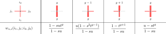
Figure 1. Vertex weights $w_{u,s}(i_{1},j_{1};i_{2},j_{2})$. Here $i_{1},i_{2}\in\mathbb{Z}_{\geq 0}$ and $j_{1},j_{2}\in\left\{0,1\right\}$.

Likewise, let us define operators $L^{*}_{v,s}$ and the corresponding weights as follows:

$$w_{v,s}^{*}(i_{1},j_{1};i_{2},j_{2})=\langle j_{2}|\otimes\langle i_{2}|\;L^{*}_{v,s}\;|j_{1}\rangle\otimes|i_{1}\rangle=\frac{(s^{2};t)_{i_{1}}(t;t)_{i_{2}}}{(s^{2};t)_{i_{2}}(t;t)_{i_{1}}}\,w_{v,s}(i_{2},j_{1};i_{1},j_{2}).$$ (2.1)

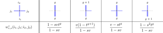
Figure 2. Vertex weights $w_{v,s}^{*}(i_{1},j_{1};i_{2},j_{2})$. Here $i_{1},i_{2}\in\mathbb{Z}_{\geq 0}$ and $j_{1},j_{2}\in\left\{0,1\right\}$.

Impose the following restrictions on the variables $u_{1},\dots,u_{N}$:

$$\left|\frac{u_{i}-s_{x}}{1-s_{x}u_{i}}\right|\leq 1-\varepsilon<1\qquad\textnormal{for all $i$ and all $x=0,1,2,\ldots$.}$$ (2.2)

Define the following transfer matrices acting on $W\otimes V$:

$$T(u) =\prod_{i=0}^{\infty}L_{u,s_{i}}=\begin{pmatrix}0&T_{+}(x)\vskip 6.0pt plus 2.0pt minus 2.0pt\\ 0&T_{-}(x)\end{pmatrix}\in{\rm End}(W\otimes V_{0}\otimes V_{1}\otimes\cdots),$$

$$T^{*}(u) =\prod_{i=0}^{\infty}L^{*}_{u,s_{i}}=\begin{pmatrix}T^{*}_{+}(x)&0\vskip 6.0pt plus 2.0pt minus 2.0pt\\ T^{*}_{-}(x)&0\end{pmatrix}\in{\rm End}(W\otimes V_{0}\otimes V_{1}\otimes\cdots).$$

See Figure 3 for an illustration.

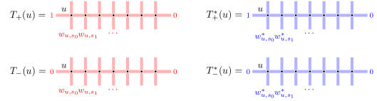
Figure 3. Graphical representation of $T$ and $T^{*}$ operators.

Remark 2.1.

Since we require the convergence condition (2.2), it follows that operators $T_{+}$ and $T^{*}_{+}$ have the vanishing property. Namely, any path that goes endlessly to the right produces the weight equal to zero, so we can forbid such paths. This means that we do not actually need to write $0$ on the right boundary in Figure 3.

Let us introduce the $R$-matrix of the six vertex model:

$$R_{z}=\begin{pmatrix}1&0&0&\frac{(1-t)z}{1-z}\\ 0&\frac{1-tz}{1-z}&0&0\\ 0&0&\frac{1-tz}{1-z}&0\\ \frac{1-t}{1-z}&0&0&t\end{pmatrix}\in{\rm End}(W\otimes W).$$

Graphically, we denote the action of this operator by cross vertices with the weights given below:

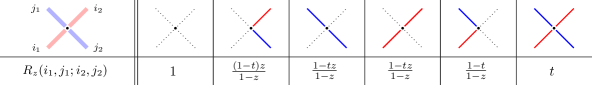
Figure 4. Cross vertex weights $R_{z}$. Here we have $i_{1},j_{1},i_{2},j_{2}\in\left\{0,1\right\}$.

Proposition 2.2 (Yang–Baxter equation).

For any $i_{1},i_{2},j_{1},j_{2}\in\left\{0,1\right\}$ and $i_{3},j_{3}\in\mathbb{Z}_{\geq 0}$ we have

$$\begin{split}&\sum_{k_{1},k_{2},k_{3}}R_{uv}(i_{2},i_{1};k_{2},k_{1})\,w^{*}_{v,s}(i_{3},k_{1};k_{3},j_{1})\,w_{u,s}(k_{3},k_{2};j_{3},j_{2})\\ &\hskip 100.0pt=\sum_{k^{\prime}_{1},k^{\prime}_{2},k^{\prime}_{3}}w^{*}_{v,s}(k^{\prime}_{3},i_{1};j_{3},k^{\prime}_{1})\,w_{u,s}(i_{3},i_{2};k^{\prime}_{3},k^{\prime}_{2})\,R_{uv}(k^{\prime}_{2},k^{\prime}_{1};j_{2},j_{1}),\end{split}$$ (2.3)

or, equivalently,

$$R_{uv}^{(12)}L^{*(1)}_{v,s}L^{(2)}_{u,s}=L^{*(1)}_{v,s}L^{(2)}_{u,s}R_{uv}^{(12)}.$$ (2.4)

Proof.

The proof is by direct computations, and we omit them. ∎

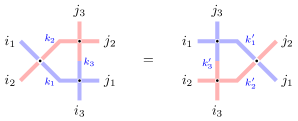
Figure 5. Graphical illustration of the Yang–Baxter equation (2.3).

Remark 2.3.

It is important that cross vertex weights in the Yang–Baxter equation (2.3) do not depend on $s$. This observation allows us to iterate this interchange relation horizontally and get an equation for $T$ and $T^{*}$ operators which is the same as (2.4) with $L_{u,s}$ and $L^{*}_{v,s}$ replaced by $T(u)$ and $T^{*}(v)$, respectively.

2.2. Spin Hall-Littlewood functions

Now we are able to give a definition of the spin Hall–Littlewood rational functions in terms of our model. Namely, they are given by the following formula:

$$F_{\lambda}(u_{1},\dots,u_{N}) =\left\langle 0\right|T_{+}(u_{1})\dots T_{+}(u_{N})\left|\lambda\right\rangle.$$

In other words, we consider the weighted sum over all the up-right paths ensembles in $\mathbb{Z}_{\geq 0}\times\left\{1,\ldots,N\right\}$ with the following properties:

1. Each path comes from the left edge and reaches the top boundary at the corresponding coordinate $\lambda_{i}$.

2. No two paths can share the same horizontal line.

3. In the vertex $(x,i)\in\mathbb{Z}_{\geq 0}\times\left\{1,\ldots,N\right\}$ we take the weight $w_{u_{i},s_{x}}$.

The example of such an ensemble is given in Figure 6.

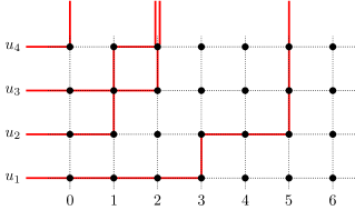
Figure 6. An example of a path configuration contributing to the partition function $F_{\lambda}(u_{1},u_{2},u_{3},u_{4})$, where $\lambda=(5,2,2,0)$.

2.3. Refinement

One can define a generalization of this partition function by adding an extra parameter $\alpha\in\mathbb{C}$. Namely, consider a vector space

$$V(\alpha)={\rm Span}\left\{\left|m_{0}+\alpha\right\rangle_{0}\otimes\left|m_{1}\right\rangle_{1}\otimes\left|m_{2}\right\rangle_{2}\otimes\cdots\right\},\qquad m_{i}\in\mathbb{Z}\ \forall\ i\geqslant 1,$$

and the corresponding family of partition functions

$$F^{\alpha}_{\lambda}(u_{1},\dots,u_{N})=\left\langle 0;\alpha\right|T_{+}(u_{1})\dots T_{+}(u_{N})\left|\lambda;\alpha\right\rangle,$$

where $\lambda$ is a signature and

$$|\lambda;\alpha\rangle=\left|m_{0}(\lambda)+\alpha\right\rangle_{0}\otimes\left|m_{1}(\lambda)\right\rangle_{1}\otimes\left|m_{2}(\lambda)\right\rangle_{2}\otimes\cdots.$$

Let $\gamma=t^{\alpha}$. Since the only difference between $F^{\alpha}_{\lambda}$ and $F_{\lambda}$ comes from different zero column weights, it is easy to express one partition function through another:

$$\begin{split}&F^{\alpha}_{\lambda}(u_{1},\dots,u_{N})=\frac{(\gamma t;t)_{m_{0}}}{(t,t)_{m_{0}}}\prod_{j=1}^{N}\frac{1-\gamma s_{0}u_{j}}{1-s_{0}u_{j}}\left[F_{\lambda}(u_{1},\dots,u_{N})\Big{|}_{\text{$s_{0}\to\gamma s_{0}$}}\right],\\ &F_{\lambda}(u_{1},\dots,u_{N})=F^{0}_{\lambda}(u_{1},\dots,u_{N}).\end{split}$$ (2.5)

3. Refined Littlewood identity. Proof.

In this section we prove the refined Littlewood identity (Theorem 1.2).

3.1. A property of the transfer matrices

Lemma 3.1.

Consider the following formal weighted sum of all states with even multiplicities:

$$\left|\rm e;\alpha\right\rangle=\sum_{\begin{subarray}{c}m_{i}(\lambda)\in 2\mathbb{Z}_{\geqslant 0}\\ m_{0}(\lambda)\in 2\mathbb{Z}\end{subarray}}\ c_{\lambda}(t;\alpha)\left|\lambda;\alpha\right\rangle,$$

where the weights are given by

$$c_{\lambda}(\alpha,t)=\prod_{i=1}^{\infty}\prod_{j=1}^{m_{i}(\lambda)/2}\frac{1-s_{i}^{2}t^{2j-2}}{1-t^{2j}}\times\left\{\begin{array}[]{cl}\displaystyle{\prod_{j=1}^{m_{0}(\lambda)/2}\frac{1-s_{0}^{2}\gamma t^{2j-2}}{1-\gamma t^{2j}}},&m_{0}(\lambda)\geqslant 0,\\ \\ \displaystyle{\prod_{j=1}^{-m_{0}(\lambda)/2}\frac{1-\gamma t^{-2j+2}}{1-s_{0}^{2}\gamma t^{-2j}}},&m_{0}(\lambda)\leqslant 0.\end{array}\right.$$

Then the transfer matrices $T_{\pm}$ and $T^{*}_{\pm}$ have the following property:

$$T_{+}\left|\rm e;\alpha\right\rangle=T^{*}_{+}\left|\rm e;\alpha\right\rangle,\quad\quad T_{-}\left|\rm e;\alpha\right\rangle=T^{*}_{-}\left|\rm e;\alpha\right\rangle.$$ (3.1)

Proof.

Take any signature $\mu$ and the corresponding state

$$\langle\mu;\alpha|=\left\langle m_{0}(\mu)+\alpha\right|_{0}\otimes\left\langle m_{1}(\mu)\right|_{1}\otimes\left\langle m_{2}(\mu)\right|_{2}\otimes\cdots$$

with $m_{0}(\mu)\in\mathbb{Z}$ and $m_{i}(\mu)\in\mathbb{Z}_{\geqslant 0}$ for all $i\geqslant 1$. Note that there exists a unique $\mu_{+}$ with even multiplicities such that $\left\langle\rm\mu;\alpha\right|T_{+}\left|\rm\mu_{+};\alpha\right\rangle\neq 0$ or $\left\langle\rm\mu;\alpha\right|T_{-}\left|\rm\mu_{+};\alpha\right\rangle\neq 0$ (which of these is nonzero depends on the parity of the sum over all the multiplicities). Also, denote by $\mu_{-}$ the unique signature with even multiplicities such that $\left\langle\rm\mu;\alpha\right|T^{*}_{+}\left|\rm\mu_{-};\alpha\right\rangle\neq 0$ or $\left\langle\rm\mu;\alpha\right|T^{*}_{-}\left|\rm\mu_{-};\alpha\right\rangle\neq 0$. For example, if $\mu=(6,4,4,3,2,2,0)$, then $\mu_{+}=(6,6,4,4,2,2,0,0)$ and $\mu_{-}=(4,4,3,3,2,2)$ (see Figure 7 for an illustration).

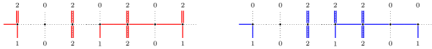
Figure 7. An illustration for the definition of $\mu_{+}$ and $\mu_{-}$ when $\mu=(6,4,4,3,2,2,0)$.

So, we obtain

$$\left\langle\rm\mu;\alpha\right|T_{\pm}\left|\rm e;\alpha\right\rangle=c_{\mu_{+}}\left\langle\rm\mu;\alpha\right|T_{\pm}\left|\rm\mu_{+};\alpha\right\rangle,\qquad\left\langle\rm\mu;\alpha\right|T^{*}_{\pm}\left|\rm e;\alpha\right\rangle=c_{\mu_{-}}\left\langle\rm\mu;\alpha\right|T^{*}_{\pm}\left|\rm\mu_{-};\alpha\right\rangle.$$

It remains to check that

$$c_{\mu_{+}}\left\langle\rm\mu;\alpha\right|T_{\pm}\left|\rm\mu_{+};\alpha\right\rangle=c_{\mu_{-}}\left\langle\rm\mu;\alpha\right|T^{*}_{\pm}\left|\rm\mu_{-};\alpha\right\rangle.$$ (3.2)

This equality can be seen from the special case of equation (2.1) and its analogue for the zero column.

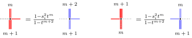
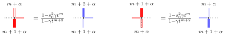
Figure 8. The correspondence between vertex weights in both sides of (3.2).

Indeed, to get $\left\langle\rm\mu;\alpha\right|T_{\pm}\left|\rm\mu_{+};\alpha\right\rangle$ with given $\left\langle\rm\mu;\alpha\right|T^{*}_{\pm}\left|\rm\mu_{-};\alpha\right\rangle$ we need to do the replacements as in Figure 8. These replacements produce some factor, meanwhile the ratio $c_{\mu_{+}}/c_{\mu_{-}}$ precisely compensates this factor. This concludes the proof. ∎

Graphically, our statement can be represented as in Figure 9.

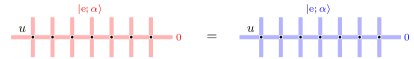
Figure 9. Graphical representation of equation (3.1). Here we do not need to specify the state on the left boundary.

3.2. Setting and transformation of the partition function

Consider the following partition function which has an additional parameter $\alpha$:

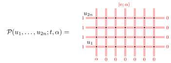
Figure 10. The left-hand side of the Littlewood identity expressed graphically as a partition function.

From the very definition we have

$$\mathcal{P}(u_{1},\dots,u_{2n};t,\alpha)=\sum_{\lambda:m_{i}(\lambda)\in 2\mathbb{Z}_{\geqslant 0}}\prod_{j=1}^{m_{0}(\lambda)/2}\frac{1-s_{0}^{2}\gamma t^{2j-2}}{1-\gamma t^{2j}}\prod_{i=1}^{\infty}\prod_{j=1}^{m_{i}(\lambda)/2}\frac{1-s_{i}^{2}t^{2j-2}}{1-t^{2j}}F^{\alpha}_{\lambda}(u_{1},\dots,u_{2n}).$$ (3.3)

Since we have up-right path ensembles and the left edge is occupied, it follows that only states with non-negative $m_{0}$ in $\left|\rm e;\alpha\right\rangle$ contribute to our summation.

Let us apply Lemma 3.1 to the upper row. We get the first equality in Figure 11.

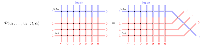
Figure 11. First step of the transformation of the partition function.

The second equality in Figure 11 holds due to the completely frozen cross part on the right, which has weight $1$.

Next, using the Yang–Baxter equation, one can move cross part of the partition to the left edge. Then we repeat this trick several times (see Figure 12 for an illustration).

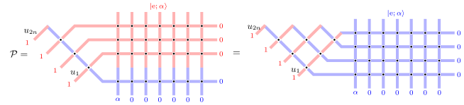
Figure 12. Next steps of the transformation of the partition function.

After moving all the crosses to the left, the partition function factorizes, and the blue frozen part on the right has weight 1. Thus, we obtain the partition function as in Figure 13.

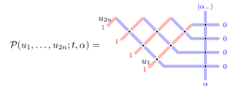
Figure 13. Expression for the left-hand side of the Littlewood identity as a partition function of the inhomogeneous six vertex model with weights $R_{u_{i}u_{j}}$ and decorated boundary conditions.

The boundary vector $\left|\rm\alpha_{-}\right\rangle$ involved there can be expressed explicitly as the following weighted sum:

$$\left|\rm\alpha_{-}\right\rangle=\sum_{k=0}^{\infty}\prod_{j=1}^{k}\frac{1-\gamma t^{-2j+2}}{1-s_{0}^{2}\gamma t^{-2j}}\left|\alpha-2k\right\rangle.$$

3.3. Properties of the partition function

Lemma 3.2.

Let $Z_{2n}$ denote the partition function $\mathcal{P}(u_{1},\dots,u_{2n};t,\alpha)$ as in Figure 13 multiplied by $\prod_{1\leqslant i<j\leqslant 2n}(1-u_{i}u_{j})\prod_{i=1}^{2n}(1-su_{i})$. Then $Z_{2n}$ possesses the following properties:

1. $Z_{2n}$ is symmetric in $\{u_{1},\dots,u_{2n}\}$.

2. $Z_{2n}$ is a polynomial in $u_{2n}$ of degree $2n-1$.

3. Setting $u_{2n}=u_{2n-1}^{-1}$, we have the recursion relation

   $$Z_{2n}|_{u_{2n}=u_{2n-1}^{-1}}=(1-t)(1-\gamma s_{0}u_{2n})(1-\gamma s_{0}u_{2n-1})\prod_{j=1}^{2n-2}(1-tu_{j}u_{2n})(1-tu_{j}u_{2n-1})Z_{2n-2}.$$

4. Under the specialization $u_{2j-1}=t$, $u_{2j}=1/t^{2}$ for $1\leqslant j\leqslant n$, we have

   $$Z_{2n}(t,1/t^{2},\dots,t,1/t^{2})=\gamma^{n}(t-1)^{n^{2}}t^{-2n}(-(t-1/t)^{2})^{n(n-1)/2}(1-s_{0}t^{-2})^{n}(1-s_{0}t)^{n}.$$

5. For $n=1$ we have

   $$Z_{2}(u_{1},u_{2})=(1-t)(1-\gamma s_{0}u_{1})(1-\gamma s_{0}u_{2})+(1-\gamma)(t-\gamma s_{0}^{2})(1-u_{1}u_{2}).$$

Proof.

To prove that $Z_{2n}$ is symmetric, let us introduce the vertex weights as in Figure 14.

Figure 14. The vertex weights $r_{z}$ and $\bar{r}_{z}$ involved in the proof of symmetry. Here $i_{1},j_{1},i_{2},j_{2}\in\left\{0,1\right\}$.

One can check that they satisfy the following Yang–Baxter equations and the unitary relation:

$$\begin{split}&\sum_{k_{1},k_{2},k_{3}}r_{u/v}(i_{2},i_{1};k_{2},k_{1})\,R_{vw}(k_{1},k_{3};j_{1},i_{3})\,R_{uw}(k_{2},j_{3};j_{2},k_{3})\\ &\hskip 100.0pt=\sum_{k^{\prime}_{1},k^{\prime}_{2},k^{\prime}_{3}}R_{vw}(i_{1},j_{3};k^{\prime}_{1},k^{\prime}_{3})\,R_{uw}(i_{2},k^{\prime}_{3};k^{\prime}_{2};i_{3})r_{u/v}(k^{\prime}_{2},k^{\prime}_{1};j_{2},j_{1}).\end{split}$$ (3.4)

$$\begin{split}&\sum_{k_{1},k_{2},k_{3}}R_{uw}(i_{3},i_{2};k_{3},k_{2})\,R_{vw}(k_{3},i_{1};j_{3},k_{1})\bar{r}_{v/u}(k_{2},k_{1};j_{2},j_{1})\\ &\hskip 100.0pt=\sum_{k^{\prime}_{1},k^{\prime}_{2},k^{\prime}_{3}}\bar{r}_{v/u}(i_{2},i_{1};k^{\prime}_{2},k^{\prime}_{1})\,R_{uw}(k^{\prime}_{3},k^{\prime}_{2};j_{3},j_{2})\,R_{vw}(i_{3},k^{\prime}_{1};k^{\prime}_{3},j_{1}).\end{split}$$ (3.5)

$$\begin{split}&\sum_{k_{1},k_{2},k_{3}}\bar{r}_{v/u}(i_{2},i_{1};k_{2},k_{1})\,w^{*}_{v,s}(i_{3},k_{1};k_{3},j_{1})\,w^{*}_{u,s}(k_{3},k_{2};j_{3},j_{2})\\ &\hskip 100.0pt=\sum_{k^{\prime}_{1},k^{\prime}_{2},k^{\prime}_{3}}w^{*}_{v,s}(k^{\prime}_{3},i_{1};j_{3},k^{\prime}_{1})\,w^{*}_{u,s}(i_{3},i_{2};k^{\prime}_{3},k^{\prime}_{2})\,\bar{r}_{v/u}(k^{\prime}_{2},k^{\prime}_{1};j_{2},j_{1}).\end{split}$$ (3.6)

$$\sum_{k_{1},k_{2},l_{1},l_{2}}r_{u/v}(i_{2},i_{1};k_{2},k_{1})\,R_{uv}(k_{1};k_{2},l_{1},l_{2})\,\bar{r}_{v/u}(l_{2};l_{1},j_{2},j_{1})=R_{uv}(i_{2},i_{1},j_{2},j_{1}).$$ (3.7)

Graphically, these equations can be viewed as in Figures 15 - 18:

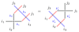
Figure 15. Graphical illustration of equation (3.4).

Figure 16. Graphical illustration of equation (3.5).

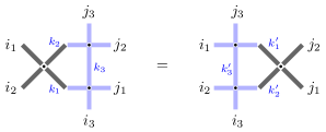
Figure 17. Graphical illustration of equation (3.6).

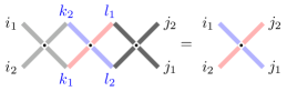
Figure 18. Graphical illustration of equation (3.7).

To see property 1, add to the partition function in Figure 13 a vertex of weight $r_{u_{i+1}/u_{i}}$ on the left at the $i$-th position, and a vertex of weight $\bar{r}_{u_{i}/u_{i+1}}$ on the right at the $i$-th position. On the one hand, these operations does not change the partition function at all. On the other hand, we can apply Yang–Baxter equations several times and the unitary relation to get the partition function with variables $u_{i}$ and $u_{i+1}$ swapped. This concludes the proof of Property 1.

For property 2 we may assume that we are considering the same partition function but with the weights $(1-u_{i}v_{j})R_{u_{i}v_{j}}$ instead of $R_{u_{i}v_{j}}$ and $(1-s_{0}u_{j})w^{*}_{u_{j}}$ instead of $w^{*}_{u_{j}}$. This makes all the weights linear, in particular, in $u_{2n}$. It allows to verify that $u_{2n}$ contributes to each part of the summation $2n-1$ times with some coefficients (independent of $u_{2n}$).

For property 3 let us notice that in this case $(1-u_{2n}u_{2n-1})R_{u_{2n}u_{2n-1}}(1,1;1,1)=0$, so we should avoid this weight at the beginning, which leads to factorization of the partition function. After some computations we get the desired property.

To prove property 4, note that the chosen $u_{1},\dots,u_{2n}$ satisfy $1-tu_{i}u_{j}=0$ for all $i,j$ such that $i+j$ is odd. So, for odd $i+j$ we have $R_{u_{i}v_{j}}(0,1,0,1)=R_{u_{i}v_{j}}(1,0,1,0)=0$ and $R_{u_{i}v_{j}}(k_{1},k_{1},k_{2},k_{2})=(-1)^{k_{1}+k_{2}}t^{k_{1}}$. This observation together with some simple freezing/combinatorial arguments implies that there are $2^{n}$ possible configurations with non-zero weights. Moreover, they are uniquely determined by values on the right edge of the six vertex model. One can compute explicitly the weight of each configuration. For example, it can be done through the following recursion relation:

$$\begin{split}&Z_{2n}(t,1/t^{2},\dots,t,1/t^{2})\\ &=(1-t)(t^{2n-1}(1-s_{0}^{2}\gamma/t)(1-\gamma)+(-t)^{2n-1}(1-s_{0}\gamma/t^{2})(1-s_{0}\gamma t))\\ &\hskip 160.0pt\times\prod_{i<2n-1}(1-u_{i}u_{2n})(1-u_{i}u_{2n-1})Z_{2n-2}(t,1/t^{2},\dots,t,1/t^{2}).\end{split}$$

Here the first and the second summands correspond to the cases where we choose $R_{u_{2n}u_{1}}(1,1,1,1)$ or $R_{u_{2n}u_{1}}(1,1,0,0)$ cross vertex weights, respectively. This recursion immediately gives us the formula:

$$Z_{2n}(t,1/t^{2},\dots,t,1/t^{2})=\gamma^{n}t^{n(n-2)}(1-s_{0}t^{-2})^{n}(1-s_{0}t)^{n}\prod_{i<j}(1-u_{i}u_{j})|_{(u_{1},...,u_{2n})=(t,1/t^{2},\dots,t,1/t^{2})}.$$

Finally, property 5 comes from direct computations. ∎

3.4. Explicit formula for the partition function

Theorem 3.3.

The partition function $\mathcal{P}(u_{1},\dots,u_{2n};t,\alpha)$ can be expressed explicitly as follows:

$$\mathcal{P}(u_{1},\dots,u_{2n};t,\alpha)=\prod_{j=1}^{2n}\frac{1}{1-s_{0}u_{j}}\prod_{1\leqslant i<j\leqslant 2n}\left(\frac{1-tu_{i}u_{j}}{u_{i}-u_{j}}\right)\mathop{\rm Pf}_{1\leqslant i<j\leqslant 2n}\left[\frac{Z_{2}(u_{i},u_{j})(u_{i}-u_{j})}{(1-u_{i}u_{j})(1-tu_{i}u_{j})}\right].$$ (3.8)

Proof.

First, one can deduce that the Pfaffian on the right-hand side of (3.8) multiplied by the product $\prod_{j=1}^{2n}(1-s_{0}u_{j})\prod_{1\leqslant i<j\leqslant 2n}(1-u_{i}u_{j})$ satisfy all the properties 1-5 from Lemma 3.2. Namely, we have property 1 because both the Pfaffian and the Vandermonde $\prod_{1\leqslant i<j\leqslant 2n}(u_{i}-u_{j})$ change the sign under swaps $u_{i}\leftrightarrow u_{i+1}$. Properties 2 and 5 are straightforward from the very definition of the Pfaffian. To get property 3, one can multiply the last row and column by $\prod_{1\leqslant j<2n}(1-u_{j}u_{2n})$ and the second-to-last row and column by $(1-u_{2n-1}u_{2n})\prod_{1\leqslant j<2n-1}(1-u_{j}u_{2n-1})$. Note that all the elements in this matrix hook vanish except two with indices $n-1$ and $n$. In turn,

$$Z_{2}(u_{2n-1},u_{2n})\big{|}_{u_{2n}=u_{2n-1}^{-1}}=(1-t)(1-\gamma s_{0}u_{2n})(1-\gamma s_{0}u_{2n-1}).$$

Likewise, one can prove property 4, using the recurrence and the following:

$$Z_{2}(t,1/t^{2})=\gamma(1-t)(1-s_{0}t^{-2})(1-s_{0}t).$$

So, it remains to show that these properties determine a function uniquely. For this purpose one can use Lagrange interpolation the same way as in [Pet21] and [WZ16, Appendix B].

Namely, we assume that two families of polynomials $f_{2n}(u_{1},\dots,u_{2n})$ and $g_{2n}(u_{1},\dots,u_{2n})$ satisfy properties 1-5 and prove that $f_{2n}=g_{2n}$ by induction on $n$. The base case follows from Property 5. To prove the induction step, assume that we proved this statement for $n-1$. Then, let us fix $2n-1$ arbitrary non-zero distinct points $u_{1},\dots,u_{2n-1}$. Using the recurrence relation and symmetry, we obtain that $f_{2n}$ and $g_{2n}$ treated as polynomials in $u_{2n}$ coincide in $2n-1$ distinct points $u_{1}^{-1},\dots,u_{2n-1}^{-1}$. Since their degree is $2n-1$, it follows that $f_{2n}-g_{2n}=c\cdot\prod_{i<j}(1-u_{i}u_{j})$ where $c$ does not depend on $u_{2n}$. However, because of symmetry it does not depend on $u_{1},\dots,u_{2n-1}$ either, which means it is an absolute constant. Finally, as can be seen from property 4, $f_{2n}$ and $g_{2n}$ have the same value at a fixed point, hence $f_{2n}=g_{2n}$.

This concludes the proof of Theorem 3.3. ∎

Corollary 3.4.

Under the specialization $u_{j}=t^{2n-j}/(\gamma s_{0})$, we have

$$\begin{split}&\mathop{\rm Pf}_{1\leqslant i<j\leqslant 2n}\left[\frac{(t^{j}-t^{i})(\gamma^{2}s_{0}^{2}(1-t)(t^{i}-t^{2n})(t^{j}-t^{2n})+(1-\gamma)(t-s_{0}^{2}\gamma)(t^{i+j}\gamma^{2}s_{0}^{2}-t^{4n})}{t^{2i+2j-2n}\gamma s_{0}(\gamma s_{0}-t^{4n}/(\gamma s_{0}))(\gamma s_{0}-t^{4n+1-i-j}/(\gamma s_{0}))}\right]\\ &=\prod_{j=0}^{2n-1}(1-t^{j}\gamma^{-1})\prod_{0\leqslant i<j\leqslant 2n-1}\left(\frac{t^{j}-t^{i}}{\gamma s_{0}-t^{i+j+1}/(\gamma s_{0})}\right)\mathcal{P}(t^{2n-1}/(\gamma s_{0}),t^{2n-2}/(\gamma s_{0}),\dots,1/(\gamma s_{0});t,\alpha)\\ &\hskip 65.0pt=(-1)^{n}\gamma^{n}t^{n^{2}}\prod_{0\leqslant i<j\leqslant 2n-1}\left(\frac{t^{j}-t^{i}}{\gamma s_{0}-t^{i+j+1}/(\gamma s_{0})}\right)\prod_{j=1}^{n}(1-s_{0}^{2}\gamma t^{-2j+1})(1-\gamma^{-1}t^{2j-2}).\end{split}$$ (3.9)

Proof.

Consider the lattice interpretation of $\mathcal{P}(t^{2n-1}/(\gamma s_{0}),\dots,1/(\gamma s_{0});t,\alpha)$. Indeed, under this specialization the right boundary is fixed, and therefore the whole configuration becomes frozen. By the way, it is not so easy to verify independently that the Pfaffian in the left-hand side of (3.9) factorizes. ∎

Using (3.3) and (2.5), the left-hand side of the identity (3.8) can be rewritten as the weighted sum of $F_{\lambda}$’s over all signatures $\lambda$ with even multiplicities in the following way:

$$\begin{split}&\sum_{\lambda:m_{i}(\lambda)\in 2\mathbb{Z}_{\geqslant 0}}\frac{1}{(t;t)_{m_{0}(\lambda)}}\prod_{j=1}^{m_{0}(\lambda)/2}(1-s_{0}^{2}\gamma t^{2j-2})(1-\gamma t^{2j-1})\prod_{j=1}^{2n}\frac{1-\gamma s_{0}u_{j}}{1-s_{0}u_{j}}\\ &\hskip 200.0pt\times\prod_{i=1}^{\infty}\prod_{j=1}^{m_{i}(\lambda)/2}\frac{1-s_{i}^{2}t^{2j-2}}{1-t^{2j}}\left[F_{\lambda}(u_{1},\dots,u_{2n})\Big{|}_{\text{$s_{0}\to\gamma s_{0}$}}\right].\end{split}$$

After replacing $\gamma s_{0}$ by $s_{0}$, we obtain the desired statement of Theorem 1.2.

4. Some specializations of the Littlewood identity

In this section we reduce our result to classical Hall–Littlewood polynomials and we write a non-refined degeneration of our result.

4.1. Reduction to the case of classical Hall–Littlewood polynomials

As was shown in [Pet21], spin Hall–Littlewood rational functions $F_{\lambda}$ can be reduced to classical Hall–Littlewood polynomials $P_{\lambda}^{HL}$ in the following way:

$$F_{\lambda}(u_{1},\dots,u_{N})\Big{|}_{\text{$s_{x}=0$}}=\prod_{r\geq 0}(t;t)_{m_{r}(\lambda)}\cdot P_{\lambda}^{HL}(u_{1},\ldots,u_{N}).$$ (4.1)

So, after setting $s_{x}=0$ in equation (1.1), we get

$$\sum_{\lambda:m_{i}(\lambda)\in 2\mathbb{Z}_{\geqslant 0}}\prod_{j=1}^{m_{0}(\lambda)/2}(1-\gamma t^{2j-1})\prod_{i=1}^{\infty}\prod_{j=1}^{m_{i}(\lambda)/2}(1-t^{2j-1})P_{\lambda}^{HL}(u_{1},\ldots,u_{2n})=\\ =\prod_{1\leqslant i<j\leqslant 2n}\left(\frac{1-tu_{i}u_{j}}{u_{i}-u_{j}}\right)\mathop{\rm Pf}_{1\leqslant i<j\leqslant 2n}\left[\frac{(u_{i}-u_{j})((1-\gamma t+(\gamma-1)tu_{i}u_{j})}{(1-u_{i}u_{j})(1-tu_{i}u_{j})}\right],$$ (4.2)

which coincides with the Littlewood identity proved in [WZ16, Theorem 5].

4.2. Reduction to the unrefined case

To get unrefined identity, we set $\gamma=1$ and obtain the following formula:

$$\sum_{\lambda:m_{i}(\lambda)\in 2\mathbb{Z}_{\geqslant 0}}\prod_{i=0}^{\infty}\prod_{j=1}^{m_{i}(\lambda)/2}\frac{1-s_{i}^{2}t^{2j-2}}{1-t^{2j}}F_{\lambda}(u_{1},\dots,u_{2n})=\\ =\prod_{1\leqslant i<j\leqslant 2n}\left(\frac{1-tu_{i}u_{j}}{u_{i}-u_{j}}\right)\mathop{\rm Pf}_{1\leqslant i<j\leqslant 2n}\left[\frac{(u_{i}-u_{j})(1-t)}{(1-u_{i}u_{j})(1-tu_{i}u_{j})}\right].$$ (4.3)

The right-hand side of (4.3) coincides with the right-hand side of (4.2) at $\gamma=1$, but the expansions are different.

S. Gavrilova, Faculty of Mathematics, National Research University Higher School of Economics, Usacheva 6, 119048 Moscow, Russia

E-mail: sveta_6117@mail.ru

References

- [BBC20] Guillaume Barraquand, Alexei Borodin, and Ivan Corwin. Half-space Macdonald processes. Forum Math. Pi, 8:150, 2020. Id/No e11.
- [BBCW18] Guillaume Barraquand, Alexei Borodin, Ivan Corwin, and Michael Wheeler. Stochastic six-vertex model in a half-quadrant and half-line open asymmetric simple exclusion process. Duke Math. J., 167(13):2457–2529, 2018.
- [BCPS15] Alexei Borodin, Ivan Corwin, Leonid Petrov, and Tomohiro Sasamoto. Spectral theory for interacting particle systems solvable by coordinate Bethe ansatz. Commun. Math. Phys., 339(3):1167–1245, 2015.
- [BCPS19] Alexei Borodin, Ivan Corwin, Leonid Petrov, and Tomohiro Sasamoto. Correction to: “Spectral theory for interacting particle systems solvable by coordinate Bethe ansatz”. Commun. Math. Phys., 370(3):1069–1072, 2019.
- [Bor17] Alexei Borodin. On a family of symmetric rational functions. Adv. Math., 306:973–1018, 2017.
- [Bor18] Alexei Borodin. Stochastic higher spin six vertex model and Macdonald measures. J. Math. Phys., 59(2):023301, 17, 2018.
- [BP18] Alexei Borodin and Leonid Petrov. Higher spin six vertex model and symmetric rational functions. Sel. Math., New Ser., 24(2):751–874, 2018.
- [BZ19] Elia Bisi and Nikos Zygouras. Point-to-line polymers and orthogonal Whittaker functions. Trans. Am. Math. Soc., 371(12):8339–8379, 2019.
- [CD21] Kailun Chen and Xiangmao Ding. Stable spin hall-littlewood symmetric functions, combinatorial identities, and half-space yang-baxter random field, 2021. arXiv:2106.12557.
- [CP16] Ivan Corwin and Leonid Petrov. Stochastic higher spin vertex models on the line. Commun. Math. Phys., 343(2):651–700, 2016.
- [CP19] Ivan Corwin and Leonid Petrov. Correction to: “Stochastic higher spin vertex models on the line”. Commun. Math. Phys., 371(1):353–355, 2019.
- [Ize87] A. G. Izergin. Partition function of a six-vertex model in a finite volume. Dokl. Akad. Nauk SSSR, 297(2):331–333, 1987.
- [KBI93] V. E. Korepin, N. M. Bogoliubov, and A. G. Izergin. Quantum inverse scattering method and correlation functions. Cambridge: Cambridge University Press, 1993.
- [KN99] A. N. Kirillov and M. Noumi. -difference raising operators for Macdonald polynomials and the integrality of transition coefficients. In Algebraic methods and -special functions, pages 227–243. Providence, RI: American Mathematical Society, 1999.
- [Kup02] Greg Kupferberg. Symmetry classes of alternating-sign matrices under one roof. Ann. Math. (2), 156(3):835–866, 2002.
- [Mac95] Ian Grant Macdonald. Symmetric functions and Hall polynomials. 2nd ed. Oxford: Clarendon Press, 2nd ed. edition, 1995.
- [Pet21] Leonid Petrov. Refined Cauchy identity for spin Hall-Littlewood symmetric rational functions. J. Comb. Theory, Ser. A, 184:50, 2021. Id/No 105519.
- [Pov13] A. M. Povolotsky. On the integrability of zero-range chipping models with factorized steady states. J. Phys. A, Math. Theor., 46(46):25, 2013. Id/No 465205.
- [RW21] Eric M. Rains and S. Ole Warnaar. Bounded Littlewood identities. Providence, RI: American Mathematical Society (AMS), 2021.
- [War06] S. Ole Warnaar. Rogers-Szegő polynomials and Hall-Littlewood symmetric functions. J. Algebra, 303(2):810–830, 2006.
- [War08] S. Ole Warnaar. Bisymmetric functions, Macdonald polynomials and basic hypergeometric series. Compos. Math., 144(2):271–303, 2008.
- [WZ16] Michael Wheeler and Paul Zinn-Justin. Refined Cauchy/Littlewood identities and six-vertex model partition functions. III. Deformed bosons. Adv. Math., 299:543–600, 2016.