Binary lattice-gases of particles with soft exclusion: Exact phase diagrams for tree-like lattices

Abstract

We study equilibrium properties of binary lattice-gases comprising $A$ and $B$ particles, which undergo continuous exchanges with their respective reservoirs, maintained at chemical potentials $\mu_{A}=\mu_{B}=\mu$. The particles interact via on-site hard-core exclusion and also between the nearest-neighbours: there are a soft repulsion between $AB$ pairs and also interactions of arbitrary strength $J$, positive or negative, for $AA$ and $BB$ pairs. For tree-like Bethe and Husimi lattices we determine the full phase diagram of such a ternary mixture of particles and voids. We show that for $J$ being above a lattice-dependent threshold value, the critical behaviour is similar: the system undergoes a transition at $\mu=\mu_{c}$ from a phase with equal mean densities of species into a phase with a spontaneously broken symmetry, in which the mean densities are no longer equal. Depending on the value of $J$, this transition can be either continuous or of the first order. For sufficiently large negative $J$, the behaviour on the two lattices becomes markedly different: on the Bethe lattice there exist two separate phases with different kinds of structural order, which are absent on the Husimi lattice, due to stronger frustration effects.

Keywords: binary lattice-gases of interacting particles, annealed disorder, order-disorder and symmetry-breaking transitions, Bethe lattice, Husimi lattice.

1 Introduction

Lattice gases of particles with on-site and also nearest-neighbour exclusion have been studied for a long time as simple models exhibiting a transition from a disordered into an ordered phase. Here, particles adsorb onto the sites of a regular lattice from a reservoir subject to the constraint that neither two particles can simultaneously occupy the same and the neighbouring lattice sites, and may desorb spontaneously back to the reservoir. A considerable knowledge of the thermodynamic properties of such systems has been gained through a series of insightful analytical and numerical analyses. Starting from the early works (see, e.g. Ref. [1] and references therein), different approaches have been proposed including, e.g. the Mayer cluster expansion [2], a variety of analyses based on the series expansions [3, 4, 5, 6, 7, 8], the quasi-chemical and ring approximations [9], the Bethe-lattice approximation [10, 11] and so on, culminating at the exact solution obtained for the so-called ”hard-hexagons” model [12, 13]. More recently, exact solutions have been found for some random graphs and also for particles that differ in size [14]. An exact solution on the Bethe lattice has been derived for a model with two kinds of particles - smaller ones which occupy a single lattice site and larger ones which do not allow other particles to occupy its neighbouring sites [15].

In this paper we are concerned with a related class of equilibrium statistical mechanics models – the so-called ”reactive” lattice gases (RLG) – in which chemical interactions between the neighbouring particles are interpreted as a nearest-neighbour exclusion constraint imposed on some kinds of particles. More specifically, there exists a special type of chemical reactions that take place whenever any two particles (similar or dissimilar, depending on the case at hand) encounter each other in a specified vicinity of a catalytic substrate. In such a situation, a reaction occurs either instantaneously or with some finite probability, and both reactants disappear from the system (see e.g. Refs. [16, 17, 18, 19, 20, 21, 22] and references therein). In RLG models one considers a regular lattice of adsorbing sites, which is in contact with a reservoir of particles (or several reservoirs, in case when several types of particles are present) maintained at a constant chemical potential; the particles thus undergo continuous exchanges with their respective reservoirs - they adsorb onto vacant lattice sites and may spontaneously desorb from the lattice. It is supposed next that either some of the lattice sites, or some of the bonds connecting neighbouring sites, have a special catalytic property such that the particles which enter into a ”reaction” cannot appear simultaneously at the neighbouring lattice sites, whenever either of them or both are catalytic, or at the neighbouring sites connected by a catalytic bond. Otherwise, in absence of a catalyst, reactive particles coexist. This reactive constraint is then interpreted in such a way that, in equilibrium, configurations of particles corresponding to a possible reaction event provide a zero contribution to the partition function, i.e. are forbidden. Note that for RLG with catalytic bonds a particle is linked by this bond to only one of its neighbours and thus ”interacts” only with it. Conversely, a particle residing on a catalytic site interacts with all of its nearest-neighbours, which results in non-additive collective interactions. We also note that, despite some similarity, there is no one-by one correspondence between the RLG models and the models of catalytic reactions introduced in Refs. [16, 17, 18, 19, 20, 21, 22]. For the latter, the presence of an irreversible reaction drives the system out-of-equilibrium, while the RLG models are defined in equilibrium.

When a lattice is completely covered by the catalytic bonds or sites, a RLG becomes a gas of hard-core particles in which the nearest-neighbour exclusion between the species which enter into a reaction is imposed on the entire lattice. For a finite concentration of the catalyst, the situation is evidently more complicated and depends also on the way how the latter is distributed on the embedding lattice. For both cases of catalytic bonds and catalytic sites present at arbitrary mean concentration, with either annealed or quenched random spatial distributions of a catalyst, exact solutions have been obtained for one-dimensional lattices for single-species [23, 24, 25, 26] and for two-species RLG [27]. In the former case, it was supposed that only one type of particles is present, while in the latter case it was assumed that there exist two dissimilar species, say $A$ and $B$, which have the same size (i.e. require a single vacant site for an adsorption) but differ in their chemical properties. Correspondingly, in the two-species case a configuration in which any $A$ and any $B$ appear at the neighbouring sites connected by either a catalytic bond, or when (at least) one of the occupied sites is in the catalytic state are forbidden, while similar species occurring at the neighbouring sites may coexist. For quenched disorder the models are solvable by combinatoric arguments or, alternatively, by expressing the adsorbate pressure as the Lyapunov index of an infinite product of random (uncorrelated for the model with catalytic bonds and sequentially correlated in case of catalytic sites) matrices. In the annealed disorder case such models reduce to those of lattice gases with a soft repulsion. One seeks then an appropriate recursion relation obeyed by the partition function and solves the latter by standard means.

For single-species RLG in higher dimensional systems the problem is clearly unsolvable in general and there exists an exact solution only for a pseudo-lattice - the so-called Bethe lattice with an annealed disorder in placement of the catalytic bonds or sites [28]. In case of catalytic bonds, the model is similar to the one studied, e.g. in Ref. [11], except for the fact that here the repulsive interactions are not infinitely strong but are ”soft” and their amplitude depends on the mean concentration $p$ of the catalytic bonds; it diverges when $p\to 1$ only, but is finite for any $p<1$. It was shown that such a model exhibits a continuous transition from a disordered into an ordered phase at a certain value of the chemical potential; evidently, for $p\to 1$ this critical value converges to the one obtained in Ref. [11]. This transition is followed by a continuous re-entrant transition into a disordered phase (which is pushed to infinity when $p\to 1$, i.e. disappears in case of hard objects). The case of catalytic sites is more complicated due to emerging multi-particle interactions and, in consequence, a critical behaviour is somewhat richer. While the direct transition into an ordered phase is always continuous, the re-entrant transition into the disordered phase may be either continuous or of the first order, depending on the value of the concentration $p_{s}$ of the catalytic sites. The critical value of the chemical potential for the re-entrant transition is also pushed to infinity as $p_{s}\to 1$.

For RLGs with two kinds of species the only available exact solution has been obtained for a regular honeycomb lattice with a random annealed distribution of the catalytic bonds in a rather special case: the chemical potentials of both species were taken equal to each other (such that both species are expected to be present, on average, at equal mean densities) and with some imposed restrictive condition that the concentration $p$ of the catalytic bonds and the interaction parameters are linked to each other through a certain relation. It was shown [29, 30] that in this special case the model reduces to an exactly solvable version of the Blume-Emery-Griffiths model, which maps onto the Ising model in a zero external field [31]. The solution then predicts a non-trivial, fluctuation-induced continuous transition into a phase with a broken symmetry with respect to the mean densities of both kinds of particles. It remains unclear, however, whether such a transition persists beyond this restrictive relation between the concentration and the interaction parameters, or it is a spurious phenomenon appearing solely due to such a constraint.

We revisit here the model considered in Refs. [29, 30] from a broader perspective by relaxing the constraint imposed on $p$ and the interaction parameters. More specifically, we study here the thermodynamic properties of a two-species RLG with reactions between dissimilar species (i.e., with an imposed constraint that dissimilar species cannot appear simultaneously on neighbouring sites connected by a catalytic bond) in the completely symmetric case in which the chemical potentials of both species involved are equal to each other, as well as are the amplitudes $J$ of interactions between the neighbouring species of the same type. One expects, of course, that in this case both species in the binary RLG are present at equal, on average, densities. The mean concentration $p$, $0\leq p\leq 1$, which defines the amplitude of the repulsive interactions between the dissimilar species, is an independent parameter, and the interaction amplitude $J$ between the neighbouring similar species is let to have an arbitrary magnitude and sign. We provide exact results for the thermodynamic properties of such binary RLGs on tree-like pseudo-lattices, as exemplified here by the Bethe lattice (see e.g. Ref. [13]) and the Husimi lattice (see e.g. Ref. [35]), with a random annealed distribution of the catalytic bonds. We note that such an analysis corresponds to a certain mean-field-like approximation of the behaviour taking place on regular lattices; we remark, however, that such an approach usually defines correctly the order of the phase transition, if any, and provides a rather accurate estimate of its location in the parameter space. We proceed to show that the symmetry breaking transition predicted in Refs. [29, 30] is a valid feature of the model, but it is not the only phase transition taking place in such a system and moreover, this transition is not always continuous. We show that for an arbitrary $p$, and for $J$ exceeding a certain positive critical value $J_{tc}(p)$ (a tricritical point), the system enters into the phase with a broken symmetry via the first order transition when the vapour pressure exceeds a certain critical value. For arbitrary $p$ and $J$ such that $J_{tc}(p)>J>J(p)$, where $J(p)$ is a $p$-dependent threshold constant, the transition into the broken-symmetry phase is continuous. Such a behaviour is predicted for both tree-like lattices, and differs only in the precise location of the demarkation curve. Behaviour at negative values of $J$, when the similar species repel each other, is very different for the Bethe and the Husimi lattices. For the Bethe lattice we realise that in certain ranges of values of $J$ and $p$ there exist two phases with a structural order: an alternating phase I in which the system spontaneously partitions into two sub-lattices - one being occupied by a mixture of both species present at equal mean densities, and the second one being almost devoid of particles, and an alternating phase II in which each of the species resides predominantly on its own sub-lattice. The system enters into such phases and leaves one of them via continuous phase transitions. On the contrary, such phases with structural order are absent on the Husimi lattice due to stronger frustration effects.

The paper is outlined as follows. In section 2 we formulate our model, derive the corresponding effective Hamiltonian and also describe the geometrical features of the tree-like lattices under study. The section 3 is devoted to the analysis of the phase diagram of the RLG and the behaviour of the characteristic parameters for the Bethe lattice. In section 4 our analysis is extended over the case of the Husimi lattice. Finally, in section 5 we conclude with a brief summary of our results. Details of intermediate derivations are relegated to Appendices.

2 Model

Consider an arbitrary lattice structure and suppose that some of the bonds connecting neighbouring sites $\langle ij\rangle$ possess a special ”catalytic” property. To specify the state of bonds, we associate with each of them a random variable $\zeta_{\langle ij\rangle}$, such that $\zeta_{\langle ij\rangle}=1$ (with probability $p$) if the bond $\langle ij\rangle$ is catalytic and $\zeta_{\langle ij\rangle}=0$, otherwise, with probability $1-p$. Hence, in the thermodynamic limit $p$ can be thought of as the mean concentration of the catalytic bonds. Suppose next that the lattice is brought in contact with two reservoirs of particles - $A$ and $B$ - which are identical in size but are distinguishable, e.g. by their colour. The reservoirs are kept at constant chemical potentials, in general, $\mu_{A}$ and $\mu_{B}$. The $A$ and $B$ particles undergo continuous exchanges with their respective reservoirs; they adsorb onto vacant lattice sites and may spontaneously desorb. Particles of similar species occurring at neighbouring sites interact with each other and the strength of such interactions is denoted by $J_{A}$ or $J_{B}$, which can be negative or positive, i.e. we let the interactions be repulsive or attractive. Lastly, we stipulate that the configurations in which an $A$ and a $B$ appear simultaneously at neighbouring sites connected by a catalytic bond are forbidden.

Let $n_{i}$ and $m_{i}$ be two Boolean variables describing an instantaneous occupation of the site $i$. We use the convention that $n_{i}=1$ ($m_{i}=1$) if the site $i$ is occupied by an $A$ (a $B$) particle, and is zero, otherwise. Situations when both $m_{i}$ and $n_{i}$ are non-zero for the same site are not permitted because of the on-site exclusion. In thermodynamic equilibrium and for a given realisation of random variables $\zeta_{\langle ij\rangle}$, the grand-canonical partition function of such a binary adsorbate, which counts the weights of different realisations of particles’ placement on the lattice, writes

$$Z(\{\zeta_{\langle ij\rangle}\}) =\sum_{\{n_{i},m_{i}\}}z_{A}^{\sum_{i}n_{i}}z_{B}^{\sum_{i}m_{i}}e^{\beta J_{A}\sum_{\langle ij\rangle}n_{i}n_{j}+\beta J_{B}\sum_{\langle ij\rangle}m_{i}m_{j}}$$

$$\times\prod_{\langle ij\rangle}(1-\zeta_{\langle ij\rangle}n_{i}m_{j})(1-\zeta_{\langle ij\rangle}m_{i}n_{j}),$$ (1)

where $\beta$ defines the reciprocal temperature measured in units of the Boltzmann constant, while $z_{A}=\exp(\beta\mu_{A})$ and $z_{B}=\exp(\beta\mu_{B})$ are the activities, associated with the chemical potentials $\mu_{A}$ and $\mu_{B}$. Further on, in equation (2), the sum with the subscript $\{n_{i},m_{i}\}$ signifies that the summation extends over all possible values of the occupation variables, while the sums (as well as the product) with the subscript $\langle ij\rangle$ denote the summation (the product) extending over all bonds connecting nearest-neighbouring lattice sites. The factor in the second line in equation (2) forbids the configurations in which an $A$ and a $B$ appear simultaneously at the neighbouring sites connected by a catalytic bond such that their contribution to the partition function equals zero.

Suppose next that the disorder in the placement of the catalytic bonds is annealed and hence, the grand-canonical partition function in equation (2) can be directly averaged over random variables $\zeta_{\langle ij\rangle}$. Because the variable $\zeta_{\langle ij\rangle}$ assigned to a given bond is statistically independent of the state of other bonds, such an averaging is straightforward and yields the following form of the grand-canonical partition function

$$Z(p) =\sum_{\{n_{i},m_{i}\}}z_{A}^{\sum_{i}n_{i}}z_{B}^{\sum_{i}m_{i}}e^{-\beta{\cal H}},$$ (2)

where ${\cal H}$ is the effective Hamiltonian of the model under study :

$${\cal H}=-J_{A}\sum_{\langle ij\rangle}n_{i}n_{j}-J_{B}\sum_{\langle ij\rangle}m_{i}m_{j}-\beta^{-1}\ln(1-p)\sum_{\langle ij\rangle}(m_{i}n_{j}+n_{i}m_{j})\,.$$ (3)

Note that upon averaging over the catalytic properties of the bonds, a strict exclusion constraint gets replaced by a milder condition: in case of an annealed disorder in placement of the catalytic bonds the dissimilar species exhibit a short-range mutual repulsion with a finite amplitude $-\ln(1-p)$, which becomes infinitely strong for $p=1$ only. Hence, for $p<1$, an $A$ and a $B$ may, in principle, reside simultaneously on the neighbouring sites but there is a penalty to pay. In what follows we will concentrate exclusively on the symmetric case with $\mu_{A}=\mu_{B}=\mu$ and $J_{A}=J_{B}=J$, such that one may expect that $A$s and $B$s are present in the system at equal mean densities. With such parameters our system maps to some kind of Blume-Emery-Griffits [32] model, known, as well as its generalizations, to describe systems with tricritical behaviour (see e.g. Refs [33, 34] and reference therein)

Our analysis of the partition function in equation (2) is performed for two particular cases of pseudo-lattices - the Bethe lattice and the Husimi lattice (see Fig. 1) [35].

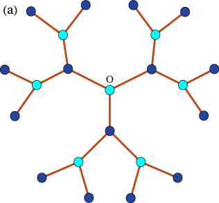
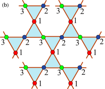
Figure 1: Panel (a). The Cayley tree with the coordination number $q=3$ containing $N=3$ generations, emanating from the root site $O$. Such a Cayley tree is bi-partite and two sub-lattices are marked by different colours. Panel (b). A fragment of the Husimi lattice with the elementary units being the triangles and the coordination number of triangles $t=2$. Such a lattice is three-partite; three different sub-lattices are denoted by $1$, $2$, and $3$, respectively.

The Bethe lattice represents a deep interior (far away of the boundary sites) of the so-called Cayley tree with an infinite number of generations (see Fig. 1, panel (a), for an example of the Cayley tree with three generations). In turn, the Husimi lattice (see Fig. 1, panel (b)) in the general case represents a deep interior part with all equivalent vertices of a connected graph whose building blocks are $Q$-polygons ($Q\geq 2$). In Fig. 1, panel (b), we depict the Husimi lattice used in our analysis for which the polygons are triangles, i.e. $Q=3$, and the coordination number $t=2$ is the number of triangles which meet at each site. Hence, the Husimi lattice under study is an infinitely nested set of corner-sharing triangles such that the local geometry is identical to that of the kagome lattice. It has, however, a weaker geometrical frustration than the original kagome lattice, because the triangles never reconnect resulting in a tree-like structure. More details about such tree-like lattices can be found in Refs. [13, 35, 36].

We close this section by mentioning that such tree-like lattices have been often used for the analysis of various models of statistical mechanics (and beyond). It was also understood in the past (see, e.g. Ref. [11]) that different approximate approaches, such as, e.g. the Bethe-Peierls approach, or some other approximations mentioned in the Introduction, correspond in fact to a replacement of the actual regular lattice by some pseudo-lattice. At the same time, the analysis performed on a pseudo-lattice provides a reliable approximation, and often a substantial improvement as compared to the mean-field calculations. The Bethe lattice approach has been employed, among many other examples, for the analysis of the phase diagram of the Blume-Emery-Griffiths model [37], of modulated phases emerging in the Ising model with competing interactions [38], the Potts model [39], lattice models of glassy systems [40] and localisation transitions [41], as well as a phase behaviour of confined ionic liquids [42, 43]. Bethe lattice approach was also used in the analytical studies of different diffusion-reaction processes [44, 45, 46], processes of random and cooperative sequential adsorption [47] or of the structural properties of branched polymers [48, 49]. The accuracy of such an approximation has been recently assessed in the numerical analysis of the Blume-Capel model and it was shown that, somewhat surprisingly, it provides a very accurate estimate of the location of the demarkation curve between the ordered and disordered phases [50]. On the other hand, the Bethe-lattice approach cannot fully reproduce the geometrical frustration in case when some competitive interactions are present, (e.g. when the coupling parameter $J$ in our model is negative and sufficiently large by its absolute value, while $z$ is sufficiently large prompting the system to accommodate more particles than the interactions permit). To incorporate the frustration effects and thus to describe the system more adequately, one devises more elaborate cluster versions in which each vertex is replaced by a frustrated geometrical unit. When the latter is taken to be a triangle, the resulting structure is precisely the Husimi tree which is considered here (see Fig. 1). Analyses of different physical models on such pseudo-lattices are quite ubiquitous and appear in various physical contexts. We just mention recent studies of antiferromagnetic classical [51, 52] and quantum spin models [53], and also several multi-site interaction models [54]. We finally remark that although such approaches usually quite accurately predict the location of the demarkation curves between ordered and disordered phase, as well as the order of the phase transition, they naturally fail to provide correct values of the critical exponents. As a matter of fact, both tree-like structures can be considered as ”infinitely-dimensional” systems, and as a consequence, they are characterised by the so-called ”mean-field” values of the critical exponents.

3 The Bethe lattice

As we have remarked above, virtually all known classical models of statistical mechanics have been studied on the Bethe lattice such that a general procedure of the derivations of the partition function is well-documented (see, e.g. Refs. [11, 13, 28]). For the case at hand, which has some interesting peculiar features, we merely present below a brief summary of the steps involved and relegate the details to the A.

Consider a Cayley tree with an arbitrary coordination number $q$ and an arbitrary number $N$ of generations (see Fig. 1 for an example with $q=3$ and $N=3$). Upon specifying the occupation of the root site $O$, the Cayley tree naturally decomposes into $q$ rooted trees, such that $Z(p)$ in equation (2) can be formally written down as

$$Z(p)=C_{N}^{q}(0,p)+z^{1-q}C_{N}^{q}(A,p)+z^{1-q}C_{N}^{q}(B,p),$$ (4)

where $C_{N}(0,p)$, $C_{N}(A,p)$ and $C_{N}(B,p)$ are the grand canonical partition functions of each rooted tree conditioned on the occupation of the root site $O$: here, the arguments $0$, $A$ and $B$ indicate that the root site is vacant, occupied by an $A$, or by a $B$ particle, respectively. In turn, each rooted tree with $N$ generations consists of $q-1$ identical subtrees with $N-1$ generations, and so on, such that a general strategy is to express the functions $C_{N}$ corresponding to a tree with $N$ generations, via the functions $C_{N-1}$ corresponding to a tree with $N-1$ generations. A derivation of the recursion relations obeyed by functions $C_{N}$ in the general case is presented in A. In the symmetric case, the latter can be conveniently written in terms of two auxiliary variables

$$x_{N}=\frac{C_{N}(A,p)}{zC_{N}(0,p)},\qquad{\text{and}}\qquad y_{N}=\frac{C_{N}(B,p)}{zC_{N}(0,p)},$$ (5)

that obey the coupled non-linear recursion scheme of the form

$$x_{N}=\frac{1+ze^{\beta J}x_{N-1}^{q-1}+(1-p)zy_{N-1}^{q-1}}{1+zx_{N-1}^{q-1}+zy_{N-1}^{q-1}},$$

$$y_{N}=\frac{1+(1-p)zx_{N-1}^{q-1}+ze^{\beta J}y_{N-1}^{q-1}}{1+zx_{N-1}^{q-1}+zy_{N-1}^{q-1}}.$$ (6)

We turn next to the limit $N\to\infty$ and consider a fragment of the Cayley tree which is in a deep interior part of a system well away from the boundary, i.e., which forms the so-called Bethe lattice [13]. The sites of the latter are all equivalent and hence, the thermodynamical phases are described by fixed point (or cycle solutions) $\{x,y\}$ of equation (3), i.e., all $\{x_{N},y_{N}\}$ should converge to $\{x,y\}$ as $N\to\infty$. Given $\{x,y\}$, one determines the ensuing thermodynamic properties of our model. In particular, the mean densities of the $A$ and $B$ species on any site of the Bethe lattice are the same, and can be expressed via the grand partition functions $C_{N}(0,p)$, $C_{N}(A,p)$ and $C_{N}(B,p)$ (see A.1) to give

$$\rho^{(A)}=\frac{zx^{q}}{1+zx^{q}+zy^{q}},\qquad\rho^{(B)}=\frac{zy^{q}}{1+zx^{q}+zy^{q}}.$$ (7)

Note finally that the derivation of the correct expression for the free energy requires some additional and rather subtle arguments, because the contributions due to the boundary sites have to be properly excluded. This procedure is described in A.2.

The subsequent analysis focuses on stability of the attractors of coupled recursions (3) for different values of the parameters $p$, $J$ and $z$. Here, four different situations are encountered:
– In some region in the parameter space two sequences $x_{N}$ and $y_{N}$ converge to a unique value $x=y$ as $N\to\infty$, which corresponds to a disordered phase with equal mean densities of $A$ and $B$ particles. In what follows, we coin such a phase as disordered symmetric phase.
– There is a domain in the parameter space in which such a convergence does not take place and instead, $x_{N}$ and $y_{N}$ converge to different limiting values $x$ and $y$ in the limit $N\to\infty$. This means, in virtue of equations (7), that here the symmetry between $A$s and $B$s is spontaneously broken and the mean densities of the components become different; one of them ($A$ or $B$ with equal probability) is present in majority with a higher mean density $\rho^{(+)}$, while the other one appears in minority with the mean density $\rho^{(-)}$, $\rho^{(+)}>\rho^{(-)}$. We call such a phase – the phase with a broken symmetry (PBS).
– There is a third situation in which $x_{N}$ ($y_{N}$) with odd $N$ converges to one value $x_{odd}$ ($y_{odd}=x_{odd}$), while for even $N$ it ultimately tends to a different value $x_{even}$ ($y_{even}=x_{even}$). Such a kind of the convergence, (the so-called subsequence convergence), is known to emerge in diverse models of statistical mechanics defined on recursive lattices. It is well-understood that, in fact, it is a manifestation of a spontaneous ordering phenomenon, i.e., an alternating partition of the particle phase, such that $A$s and $B$s occupy predominantly just one of two sub-lattices, while the second sub-lattice is almost empty. In this phase the mean densities of both species are equal to each other but there is a structural order. In what follows, we refer to such a phase as a symmetric phase with an alternating order I (PAO I).
– For some values of the parameters a fourth situation is realised in which $x_{N}$ with odd $N$ and $y_{N}$ with even $N$ converge to one value $x_{odd}=y_{even}$, while $x_{N}$ for even $N$ and $y_{N}$ for odd $N$ tend to a different value $x_{even}=y_{odd}$. Physically, it corresponds to a situation, in which $A$s occupy predominantly one of the sub-lattices, while $B$s reside on the second one. Here, the mean densities of both species are also equal to each other. We refer to such a phase as a symmetric phase with an alternating order II (PAO II).
A salient feature of two last situations is that there are corresponding phase transitions: at entering the PAO I from a symmetric disordered phase, and while leaving it to (or re-entering) a symmetric disordered phase. Similarly, there is a continuous transition upon entering the PAO II. Here, to tackle analytically an emerging subsequence convergence, one reiterates the recursions (3) expressing $x_{N}$ and $y_{N}$ through $x_{N-2}$ and $y_{N-2}$, (instead of $x_{N-1}$ and $y_{N-1}$), such that $N$ and $N-2$ appear to have the same parity. Then, the analysis proceeds in the same way as for the symmetric disordered phase or the phase with a broken symmetry, i.e. one goes to the limit $N\to\infty$ and concentrates on the sites which belong to the Bethe lattice. The order of the transitions which take place while crossing the demarkation line between different phases is obtained in a standard way from the analysis of the behaviour of the free energy (see equation (41)) and of the thermodynamic properties at the transition points.

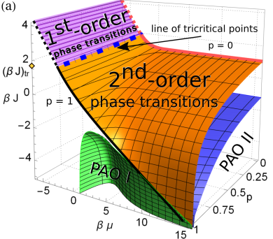
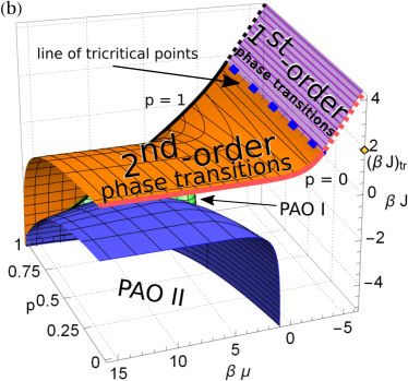
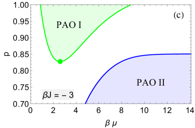
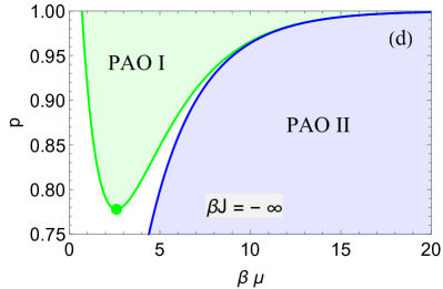
Figure 2: (Colour online) Panel (a) : Phase diagram in the parameter space ($J,\mu,p$) for the Bethe lattice with the coordination number $q=3$. The shaded surface divides the parameter space into two sub-spaces: the one above the surface corresponds to a phase with a broken symmetry (PBS) (see also panels (b) in Figs. 3 and 4), while below one has a symmetric phase with equal $A$ and $B$ particles densities. The thick red and thick black curves indicate the crossings of the demarkation surface with the $p=0$ and $p=1$- planes. A part of the shaded surface (purple) above the thick dash-dotted curve (blue) – the line of tricritical points – corresponds to the first order transition into the PBS, while below this curve (a part of the surface painted by orange colour) the transition is continuous ($2^{\rm nd}$ order). Shaded surfaces within the symmetric disordered phase bound phases with an alternating order (PAO): the PAO I, in which $A$s and $B$s both occupy predominantly either of the sub-lattices, the second one being almost empty, is inside the green one, while the blue one envelopes the PAO II, in which the two species separate residing predominantly on two different sub-lattices. The panel (b) depicts the phase diagram on the panel (a) rotated on $90^{\circ}$, to make apparent the PAO II. Panels (c) and (d) present the phase diagrams on the $(p,\mu)$-plane for two fixed values of $J$: $\beta J=-3$ (c) and $\beta J=-\infty$ (d), i.e., for an infinitely strong repulsion between similar species. Filled (green) circles denote the critical value $p_{c,1}$ of the parameter $p$, below which the PAO I does not exist; $p_{c,1}\approx 0.8276$ (c) and $p_{c,1}=7/9$ (d). For $p\geq p_{c,1}$, the PAO I exists for $\beta\mu$ within the interval $(\beta\mu)_{c,1}\leq\beta\mu\leq(\beta\mu)_{c,2}$, equations (13)) and (14). The PAO II occurs for $\beta\mu>(\beta\mu)_{c,3}$, equation (15), and $p\leq p_{c,2}$. In particular, $p_{c,2}\approx 0.8506$ for $\beta J=-3$ (c) and $p_{c,2}=1$ for $\beta J=-\infty$ (d).

The analysis of solutions of coupled recursion schemes (3) permits us to construct the full phase diagram of our model on the Bethe lattice. We depict it in Fig. 2 for the particular case $q=3$. More general results for arbitrary $q\geq 3$ and details of calculations are presented in A. Note that the results for $q=3$ and $q>3$ are qualitatively similar and differ only in the precise values of the parameters at which a critical behaviour takes place. The phase diagram for $q=3$ is presented in the space of three parameters: interaction strength $J$, chemical potential $\mu$ and the mean density $p$ of the catalytic bonds, which controls the amplitude of repulsive interactions between neighbouring dissimilar species. The phase diagram shows that a binary lattice-gas of particles with such interactions can be either in a symmetric phase, in which the mean densities of $A$ and $B$ particles are equal to each other, or in a phase in which such a symmetry is broken - the PBS, in which the mean densities of both species are no longer equal. Moreover, our analysis reveals that the symmetric phase itself divides into three sub-phases: a disordered symmetric phase and symmetric phases with two types of structural alternating order (PAO I and PAO II), the properties of which will be discussed at the end of this section.

3.1 Symmetric phase versus the phase with a broken symmetry (PBS).

The symmetric phase and the PBS are separated by a demarkation surface defined as an implicit solution of equations (50) and (55), which are presented in A. The PBS is situated above the demarkation surface, while the symmetric phase in which the mean densities of the $A$ and $B$ particles are equal to each other is below this surface.

On this surface, there exists a line of tricritical points defined by

$$(\beta J)_{tc}=\ln\left(4-p+{\sqrt{9-4p(1-p)}}\right)\,.$$ (8)

The value of $\beta J$ at the tricritical point is thus a slowly (logarithmically) varying function of the mean density of the catalytic bonds; in particular, for $p=0$, (such that there is no repulsion between neighbouring $A$s and $B$s), we have $(\beta J)_{tc}=\ln(7)\simeq 1.946$. For $p=1$, (such that $A$s and $B$s are not allowed to occupy the neighbouring sites), $(\beta J)_{tc}=\ln(6)\simeq 1.792$. For intermediate values of $p$, the value of the interaction strength $(\beta J)_{tc}$ at the tricrital point smoothly interpolates between these two (not very different) numbers. Note that $(\beta J)_{tc}$ is always positive, such that the tricritical points exist only in case of attractive interactions between similar species.

Suppose next that we fix $\beta\mu$ (or the activity $z$) and $p$, and vary $\beta J$ from some large negative value to a positive one, such that for a certain value of $\beta J$ we cross the demarkation surface. This critical value, i.e. $(\beta J)_{c}$ corresponds to a transition point from a phase with equal densities of the $A$ and $B$ particles to the PBS. If such a crossing occurs above the line of tricritical points, the transition is of the first order and manifests itself via a discontinuity in the values of densities, while a crossing below this line corresponds to a continuous ($2^{\rm nd}$ order) transition. Similarly, if we fix $p$ and $\beta J>J(p)$, where $J(p)$ is some $p$-dependent threshold value of the strength of interactions between similar species:

$$\beta J(p)=\ln\left(3(1-p)\right)\,,$$ (9)

and increase $\beta\mu$ from some large negative value to a sufficiently large positive value, we make the system to undergo a phase transition into the PBS. The order of a transition depends on the values of $p$ and $\beta J$ : if $\beta J>(\beta J)_{tc}$, equation (8), the transition is of the first order, while for $\beta J(p)<\beta J<(\beta J)_{tc}$ the transition is continuous and happens at the value of the activity which is equal to

$$z_{c}=\exp\left((\beta\mu)_{c}\right)=\frac{(e^{\beta J}+3p-1)^{2}}{4(e^{\beta J}-3(1-p))(e^{\beta J}-1+p)^{2}}.$$ (10)

For $\beta J<\beta J(p)$, equation (9), (which inequality can also be re-interpreted as some restriction imposed on the value of $p$), no such transition takes place and the system remains in the symmetric phase for any value of $\beta\mu$. It follows from equation (10) that for $p=0$ the critical value of the activity is simply $z_{c}=1/(4(\exp(\beta J)-3))$, (see the thick red curve in Fig. 2), and hence, no transition takes place for such a value of $p$ for $\beta J<\ln(3)$. In the opposite limit, i.e., for $p\to 1$, (see the thick black curve in Fig. 2), $J(p)\to-\infty$ and hence, a transition exists for any sign and value of $J$.

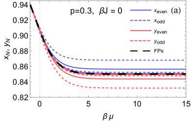
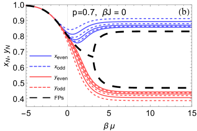
Figure 3: (Colour online) Solutions $x_{N}=x_{N}(J,\mu,p)$ (blue curves) and $y_{N}=y_{N}(J,\mu,p)$ (red curves) of the recursion relations (3) with $J=0$ and $q=3$ for $N=3,\ldots 8$, plotted as function of $\beta\mu$. Solid (dashed) curves correspond to even (odd) $N$. The initial values are $x_{0}=1$ and $y_{0}=0$. Thick dashed curves (black) present the limiting ($N\to\infty$) solutions $x$ and $y$ - the fixed point (FP) solutions. Panel (a): $p=0.3$. $x_{N}$ and $y_{N}$ converge to the same value $x=y$ in the limit $N\to\infty$ (see equation (50)). Panel (b): $p=0.7$. Spontaneous breaking of a symmetry at $\beta\mu_{c}$, equation (11), followed by a transition into the PBS – $x_{N}$ and $y_{N}$ converge to limiting values $x\neq y$ (see equations (55) and (57)).

To illustrate the above general discussion with a particular example, let us consider the case $J=0$, i.e., the case in which the similar species do not have any other interaction between themselves apart from the hard-core one. In this case, evidently, one may have only a continuous transition because $(\beta J)_{tc}$ is always greater than zero. Moreover, a continuous transition may only occur if $J(p)<0$, which imposes some restrictions on the value of $p$: it has to exceed the critical value $p^{\rm(Bet)}=2/3$, (where the superscript ${\rm(Bet)}$ signifies that this critical value is specific to the Bethe lattice). Otherwise, for $p<p^{\rm(Bet)}$ the system will not exhibit any transition for any value of the chemical potential and will remain in the symmetric phase. For $p>p^{\rm(Bet)}$, conversely, there will occur a continuous transition into the phase with a broken symmetry for $z$ equal to

$$z_{c}=e^{(\beta\mu)_{c}}=\frac{9}{4(3p-2)}.$$ (11)

In Fig. 3 we illustrate different kinds of a convergence to the limiting behaviour in the cases when $p<p^{\rm(Bet)}$ or $p>p^{\rm(Bet)}$. To this end, we present the solutions $x_{N}$ and $y_{N}$ of recursion relations (3) with $J=0$ and $q=3$, for several low order values of $N$, $N=3,\ldots 8$. We observe that for $p<p^{\rm(Bet)}$ (Fig. 3, panel (a)) the solutions $x_{N}$ and $y_{N}$ converge with a growth of $N$ to the same ultimate value $x=y$ – the fixed point solution, depicted by a thick dashed black curve – for any value of $\beta\mu$. Moreover, we conclude that only the lowest order solutions deviate from the fixed point solution in a noticeable way; $x_{1}$ (dashed blue curve) and $x_{2}$ (solid blue curve) appear to be slightly above the latter, while $y_{1}$ (dashed red curve) and $y_{2}$ (solid red curve) are slightly below the fixed point solution. The solutions with larger $N$ get progressively closer and eventually become almost indistinguishable from the fixed point solution. Concurrently, for $p>p^{\rm(Bet)}$ (Fig. 3, panel (b)) such a convergence takes place only for moderate values of $\beta\mu$, i.e., for $\beta\mu<(\beta\mu)_{c}$, equation (11). For $\beta\mu$ exceeding the critical value in equation (11), a breaking of a symmetry between $x$ and $y$ takes place such that $x_{N}$ approach from above the upper branch of the fixed point solution (here, the curves for progressively larger $N$ are ordered from top to bottom), while $y_{N}$ approach from below the lower branch (here, the curves for progressively larger $N$ are ordered from bottom to top). We note that the fact that, upon a breaking of the symmetry, $x_{N}$ appears to be larger than $y_{N}$ (but not vice versa), is due to the initial condition that we have chosen here; that being, $x_{0}=1$ and $y_{0}=0$. We note, as well, that the convergence in the region with a broken symmetry is visibly much slower. Indeed, the solutions with the largest considered $N$, i.e., $x_{8}$ and $y_{8}$, are still quite far from the fixed point solutions even far away from the transition point. Evidently, the convergence is slowest in the vicinity of the latter.

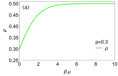
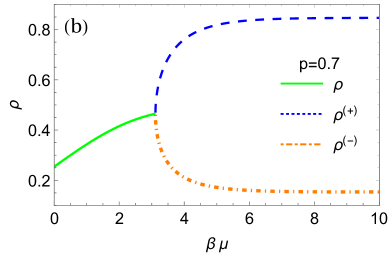
Figure 4: (Colour online). Mean densities of hard-core ($J=0$) $A$ and $B$ particles on the Bethe lattice with $q=3$ as functions of $\beta\mu$ for two values of $p$. Panel (a): $p=0.3<p^{\rm(Bet)}$ and panel (b): $p=0.7>p^{\rm(Bet)}$. The solid (green) curve shows the mean particles’ density $\rho=\rho^{(A)}=\rho^{(B)}$ in the symmetric phase, in which they are equal to each other. The dashed (blue) and the dash-dotted (orange) curves in panel (b) show the mean particles’ densities $\rho^{(+)}$ and $\rho^{(-)}$ within the PBS (see equations (3.1)).

Such a behaviour of solutions of the recursion relations (3), in virtue of equation (7) relating $x$ and $y$ to the mean densities, is evidently translated into a similar behaviour of the latter. In Fig. 4 we depict the dependence of the mean densities on $\beta\mu$ for these chosen cases. We observe that for $p=0.3$, (which is below $p^{\rm(Bet)}=2/3$), the densities of both species are equal to each other and increase monotonically from zero to the limiting value $1/2$, (when $\beta\mu$ is varied from $-\infty$ to $+\infty$), showing that the repulsive interactions between the dissimilar species are not sufficiently strong to prevent a complete coverage of the system. The penalty one has to pay for having an $A$ and a $B$ at the neighbouring sites is paid here by the chemical potential. Conversely, for $p=0.7$, (which exceeds $p^{\rm(Bet)}=2/3$), the situation appears to be different; here, the mean densities of both species are equal to each other for moderate values of $\beta\mu$, and then, when $\beta\mu$ approaches a critical value $(\beta\mu)_{c}$ (see equation (11)), a spontaneous symmetry-breaking occurs and within the PBS the densities are no longer equal. If we keep on increasing $\beta\mu$, both densities will approach their ultimate values that depend on the value of $p$:

$$\rho^{(+)}\Big{|}_{(\beta\mu)\to\infty} = \frac{1}{2}+\frac{1}{2}\frac{\sqrt{(8-3p)p-4}}{\Big{(}(5-2p)p-2\Big{)}},$$

$$\rho^{(-)}\Big{|}_{(\beta\mu)\to\infty} = \frac{1}{2}-\frac{1}{2}\frac{\sqrt{(8-3p)p-4}}{\Big{(}(5-2p)p-2\Big{)}},$$ (12)

where the function under the radical is positive for $p>p^{\rm(Bet)}$ and vanishes at $p=p^{\rm(Bet)}$. It is worthy to note that $\rho^{(+)}$ ($\rho^{(-)}$) is a monotonically increasing (decreasing) function of $p$ and the maximal value $\rho^{(+)}=1$ ($\rho^{(-)}=0$) is achieved only for $p=1$ and $\beta\mu=\infty$, i.e. for an infinitely strong repulsion between dissimilar species and for an infinitely large chemical potential. However, for $p^{\rm(Bet)}<p<1$, the breaking of the symmetry is not complete even for $\beta\mu\to\infty$ and some amount of the minority species is present. We also note parenthetically that values of the mean densities corresponding to zero chemical potential (i.e., for $z=0$) only very slightly deviate from $1/3$ for both cases: $\rho\approx 0.2993$ (for $p=0.3$) and $\rho\approx 0.2543$ (for $p=0.7$) (see also C).

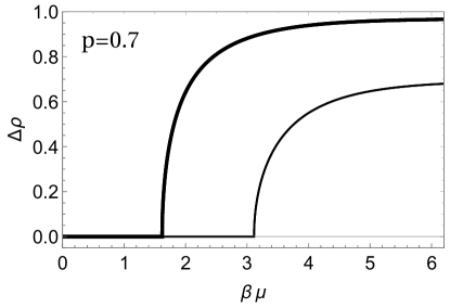
Figure 5: Order parameter $\Delta\rho$ for $J=0$ and $p=0.7$ as function of $\beta\mu$. Thin curve shows the result for the Bethe lattice (see equation (61) in the A), while the thick curve presents an analogous result for the Husimi lattice, equation (29).

Further on, it might also be instructive to check how fast the densities depart from each other upon a transition into the PBS. To this end, we depict in Fig. 5 (thin curve) the absolute value $\Delta\rho$ of the difference of $\rho^{(A)}$ and $\rho^{(B)}$, $\Delta\rho=|\rho^{(A)}-\rho^{(B)}|$, as a function of $\beta\mu$, which is the natural order parameter in the model under study. Obviously, $\Delta\rho$, which is explicitly defined in equation (61) in A, is identically equal to zero in the symmetric phase and becomes non-zero in the PBS. We observe that the growth of $\Delta\rho$ for $\mu>\mu_{c}$ is rather steep; we show analytically in A.4 that the order parameter behaves as $\Delta\rho\sim(\mu-\mu_{c})^{1/2}$ in the vicinity of $\mu=\mu_{c}$. As we have already remarked, this is a mean-field-type prediction for the value of the critical exponent in case of a continuous transition, which is the consequence of the fact that the Bethe-lattice is an effectively infinitely dimensional system. In A.4 we show, as well, that when a transition into the PBS takes place at the line of the tricritical points, $\Delta\rho\sim(\mu-\mu_{c})^{1/4}$ in the vicinity of $\mu=\mu_{c}$, which is another well-known ”mean-field ”value of the critical exponent.

3.2 Symmetric phase with a structural order

We note now that the discussion in the previous subsection does not provide an exhaustive picture, as one may infer, e.g., from Fig. 6, in which we depict low order ($N=3,\ldots,8$) solutions of recursion relations (3) with $q=3$, $p=0.9$ and $\beta J=-5$, (i.e., there is a rather strong repulsion between both similar and dissimilar species), plotted as functions of $\beta\mu$. Inspecting the recursion relations (3) further, we realise that there exist two regions in the parameter space situated well within the symmetric phase, (both regions emerge at sufficiently large negative $\beta J$), in which $x_{N}$ and $y_{N}$ with $N$ odd and with $N$ even converge to different limiting curves, while we still have $x_{N}=y_{N}$ as $N\to\infty$, i.e., the mean densities of both species are the same. In other words, in these regions there is no breaking of a symmetry between the mean particles’ densities as observed in Sec. 3.1, but instead some kind of a structural order emerges, that manifests itself via a breaking of the symmetry between the solutions that have a different parity. As we have already mentioned, the point is that here the system (recall that the Bethe lattice is a bipartite lattice) partitions spontaneously into two different sub-lattices with different particles’ arrangements on each of them, and solutions with even $N$ define the occupation of one of the sub-lattices, while the solutions with odd $N$ - the occupation of the other one. We show in what follows that these special regions correspond to the phases with an alternating order: one of them is the phase (PAO I) in which both $A$s and $B$s appear predominantly on the same sub-lattice, leaving the second sub-lattice almost empty, while in the second phase (PAO II) the $A$ particles occupy predominantly one sub-lattice, while $B$s appear mostly on the second one.

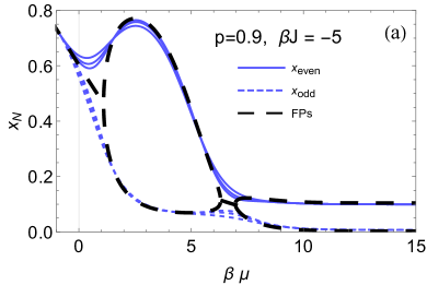
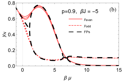
Figure 6: (Colour online) Solutions $x_{N}=x_{N}(J,\mu,p)$ (panel (a)) and $y_{N}=y_{N}(J,\mu,p)$ (panel (b)) of the recursion relations (3) with $q=3$, $p=0.9$, and $\beta J=-5$, plotted as functions of $\beta\mu$. Initial conditions are $x_{0}=1$ and $y_{0}=0$. Solid curves correspond to even $N$, the dashed ones - to odd $N$, respectively, while the thick (black) dashed curve depicts the fixed point solution. For $\beta\mu<(\beta\mu)_{c,1}(p,J)$ and $(\beta\mu)_{c,2}(p,J)<\beta\mu<(\beta\mu)_{c,3}(p,J)$ (see equations (13), (14) and (15)), $x_{N}$ and $y_{N}$ converge to the same fixed point solution $x=y$, regardless of the parity of $N$, which corresponds to the symmetric disordered phase. Within the interval $(\beta\mu)_{c,1}(p,J)<\beta\mu<(\beta\mu)_{c,2}(p,J)$, $x_{N}$ and $y_{N}$ with odd $N$ converge to $x_{odd}=y_{odd}$ as $N\to\infty$, while the solutions with even $N$ converge in this limit to $x_{even}=y_{even}$, respectively. This region defines the alternating order phase PAO I, in which $A$s and $B$s occupy predominantly one of the sub-lattices, leaving the second one almost empty. For $\beta\mu>(\beta\mu)_{c,3}(p,J)$ a different kind of a convergence takes place when $x_{N}$ with even $N$ and $y_{N}$ with odd $N$ converge to the same limiting curve $x_{even}=y_{odd}$, while $x_{N}$ with odd $N$ and $y_{N}$ with even $N$ converge to $x_{odd}=y_{even}$. This region defines the alternating order phase – PAO II, in which similar species occupy predominantly the same sub-lattice.

More specifically, there exist (see A for the derivation) three critical values of the activity $z$ (the logarithms of which define the corresponding critical values of the chemical potential),

$$z_{c,1}(p,J){=}\frac{3p(6{-}p){-}11{-}3\,e^{2\beta J}{-}6(3{-}p)e^{\beta J}{-}\sqrt{\left(9p{-}7{-}9\,e^{\beta J}\right)\left(1{+}p{-}e^{\beta J}\right)^{3}}}{8\left(1{-}p{+}e^{\beta J}\right)^{3}},$$ (13)

$$z_{c,2}(p,J){=}\frac{3p(6{-}p){-}11{-}3\,e^{2\beta J}{-}6(3{-}p)e^{\beta J}{+}\sqrt{\left(9p{-}7{-}9\,e^{\beta J}\right)\left(1{+}p{-}e^{\beta J}\right)^{3}}}{8\left(1{-}p{+}e^{\beta J}\right)^{3}},$$ (14)

and

$$z_{c,3}(p,J)=\frac{(3e^{\beta J}+p-3)^{2}}{4(e^{\beta J}+p-1)^{2}(1-3e^{\beta J}-p)},$$ (15)

which delineate the boundaries of the phases with an alternating order. We now dwell some more on the loci and properties of these phases.

(i) The disordered symmetric phase exists only when $\beta\mu<(\beta\mu)_{c,1}(p,J)$ or when $\beta\mu$ is within the bounded interval $(\beta\mu)_{c,2}(p,J)<\beta\mu<(\beta\mu)_{c,3}(p,J)$. In this range of values of the chemical potential solutions of the recursion relations (3), regardless of the parity of $N$, converge to the same value $x=y$ which is the fixed point solution. This implies that here, in virtue of equation (7), $\rho^{(A)}=\rho^{(B)}$.

(ii) When $\beta\mu$ exceeds $(\beta\mu)_{c,1}(p,J)$ the system enters, via a continuous transition, into the PAO I in which the symmetry between solutions with a different parity is broken. Indeed, here we have that $x_{N}$ ($y_{N}$) with even $N$ and with $N$ odd converge to different limiting curves – $x_{even}$ ($y_{even}=x_{even}$) and $x_{odd}$ ($y_{odd}=x_{odd}$). For example, we observe in Fig. 6 that for $\beta\mu\approx 3$ the solutions $x_{even}$ and $y_{even}$ attain their maximal value $x_{even}=y_{even}\approx 0.8$, while $x_{odd}$ and $y_{odd}$ are close to their minimal value, $x_{odd}=y_{odd}\approx 0.1$. This implies that, in virtue of equation (7), on one of the sub-lattices we have $\rho^{(A)}=\rho^{(B)}\approx 0.48$, i.e., a very high coverage by both species which are present in equal amounts, while on the second one we have $\rho^{(A)}=\rho^{(B)}\approx 0.02$, i.e., this sub-lattice is almost completely devoid of particles. The system leaves this phase and re-enters the symmetric disordered phase, again via a continuous transition, when $\beta\mu=(\beta\mu)_{c,2}(p,J)$.

We note now that $z_{c,1}(p,J)$ and $z_{c,2}(p,J)$ in equations (13) and (14) have to be real positive numbers. This latter condition implies that there are some restrictions on the values of $p$ and $J$. Namely, the PAO I may only exist when $p$ and $\beta J$ obey simultaneously

$$p\geq p_{c}=\frac{7}{9}+e^{\beta J}\,,\quad\beta J\leq\ln\left(2/9\right)\,,$$ (16)

which inequalities define the location of this phase on the phase diagram in Fig. 2.

(iii) At $\beta\mu=(\beta\mu)_{c,3}(p,J)$ the system enters, via a continuous transition, from the symmetric disordered phase into the PAO II and stays within this phase for any $\beta\mu\in((\beta\mu)_{c,3}(p,J),\infty)$, i.e., extends to infinitely large values of the chemical potential. As can be seen in Fig. 6, in this phase a salient feature is that, while the solutions $x_{N}$ with $N$ even and with $N$ odd maintain their order in the sense that $x_{even}>x_{odd}$, likewise it happens within the PAO I, the solution $y_{N}$ with $N$ even chooses here the lower branch of the fixed point solution, while the solution with $N$ odd selects the upper branch, such that $y_{odd}>y_{even}$ in the PAO II. Hence, there is a spontaneous breaking of the symmetry between the solutions with a different parity such that the system partitions into two sub-lattices, but particles’ arrangements on each of the sub-lattices is completely different, as compared to the one in PAO I. Suppose that we take $\beta\mu=10$, which is well within this phase. Then, we have that here $x_{even}=y_{odd}\approx 0.09$ and $x_{odd}=y_{even}\approx 0.01$. From our equation (7) it follows then that on one of the sub-lattices $\rho^{(A)}\approx 0.48$ and $\rho^{(B)}\approx 0.02$, while on the other - $\rho^{(A)}\approx 0.02$ and $\rho^{(B)}\approx 0.48$. Therefore, the PAO II is the phase with an alternating structural order but here the system splits into two sub-lattices each of which is predominantly occupied by just one kind of species.

For the PAO II to exist, it is necessary that the critical activity $z_{c,3}(p,J)$ in equation (15) is a real positive number. This can only be realised for such values of $p$ and $J$ which obey the inequality

$$1-3e^{\beta J}-p\geq 0\,,$$ (17)

which, together with the condition $\beta\mu\geq(\beta\mu)_{c,3}(p,J)$, defines the location of the PAO II on the phase diagram in Fig. 2.

Lastly, we note that the passage from the PAO I to PAO II, upon an increase of the chemical potential, proceeds via a transition through the symmetric disordered phase. Leaving the PAO I, the system thus looses the structural order I and becomes disordered. It regains a structural order of a different kind upon entering the PAO II. One can straightforwardly verify that the difference $(\beta\mu)_{c,3}(p,J)-(\beta\mu)_{c,2}(p,J)$, which defines the range of values of the chemical potential in which the system is in the disordered phase, is always positive and finite. This difference vanishes only for systems with $p=1$, (i.e., for an infinitely strong repulsion between dissimilar species), when, additionally, one goes to the limit of an infinitely strong repulsion between similar species, i.e., $J\to-\infty$.

4 The Husimi lattice

In this section we consider our model on the Husimi tree (see Fig. 1, panel (b)). In our analysis, we proceed along the same lines as it was done in case of the Bethe lattice. We first evaluate appropriate recursion relations, obeyed by the partition function and then turn to the limit $N\to\infty$ concentrating on the behaviour of the interior sites which are far away from the boundary. This geometrical construction represents the so-called Husimi lattice. Our derivations of the recursion relations are performed for arbitrary $J_{A}$, $J_{B}$, $z_{A}$ and $z_{B}$, and $t$ - the number of triangles that meet each other at each vertex. The final results are presented and discussed solely for the symmetric case with $J_{A}=J_{B}=J$ and $z_{A}=z_{B}=z$, and also for the simplest non-trivial geometry with $t=2$, which corresponds to an approximation of the so-called kagome lattice.

We first write formally $Z(p)$ in equation (2) defined on the Husimi tree in form of equation (4), i.e. consider three possible events with respect to the occupation of the root site,

$$Z(p)=D_{N}^{t}(0,p)+z_{A}^{1-t}D_{N}^{t}(A,p)+z_{B}^{1-t}D_{N}^{t}(B,p)\,,$$ (18)

where $D_{N}(0,p)$, $D_{N}(A,p)$ and $D_{N}(B,p)$ are, respectively, the grand canonical partition functions of a single branch with a root site which is vacant, occupied by an $A$ particle, or occupied by a $B$ particle. Recursion relations obeyed by these conditional grand canonical partition functions are listed in the B (see equations (75) and (76)).

Introducing next auxiliary variables

$$x_{N}=\frac{D_{N}(A,p)}{z_{A}D_{N}(0,p)},\qquad{\text{and}}\qquad y_{N}=\frac{D_{N}(B,p)}{z_{B}D_{N}(0,p)},$$ (19)

we find that they obey (for arbitrary $J_{A}$, $J_{B}$, $z_{A}$, $z_{B}$ and $t$) the following recursions:

$${x}_{N} {=} \frac{1{+}2e^{\beta J_{A}}\xi{+}2(1{-}p)\eta{+}2(1{-}p)^{2}e^{\beta J_{A}}\xi\eta{+}e^{3\beta J_{A}}\xi^{2}{+}(1{-}p)^{2}e^{\beta J_{B}}\eta^{2}}{1{+}2\xi{+}2\eta{+}2(1{-}p)\xi\eta{+}e^{\beta J_{A}}\xi^{2}{+}e^{\beta J_{B}}\eta^{2}},$$

$${{y}}_{N} {=} \frac{1{+}2(1{-}p)\xi{+}2e^{\beta J_{B}}\eta{+}2(1{-}p)^{2}e^{\beta J_{B}}\xi\eta{+}e^{3\beta J_{B}}\eta^{2}{+}(1{-}p)^{2}e^{\beta J_{A}}\xi^{2}}{1{+}2\xi{+}2\eta{+}2(1{-}p)\xi\eta{+}e^{\beta J_{A}}\xi^{2}{+}e^{\beta J_{B}}\eta^{2}},$$ (20)

with notations $\xi=z_{A}x_{N-1}^{(t-1)}$ and $\eta=z_{B}y_{N-1}^{(t-1)}$. Equations (4) have a substantially more complicated form (even in the symmetric case) than their counterparts in equations (3), evaluated for the Bethe lattice.

We next turn to the limit $N\to\infty$ and consider only the sites which are deep inside the Husimi tree, (i.e. belong to the Husimi lattice). Then, we realise that the recursion relations (4) converge to some fixed point solutions $x$ and $y$, which may be equal to each other or have unequal values, and thus correspond to different thermodynamic phases. From now on we concentrate on the symmetric case and also set $t=2$.

As in case of the Bethe lattice (see the A), the subsequent analysis is conveniently performed in terms of variables $u=(x+y)/2$ and $v=(x-y)/2$. Changing the variables $x$ and $y$ in equations (4) for $u$ and $v$, we find that the latter obey non-linear equations of the form

$$u {=}\frac{1{+}2z\left(1{-}p{+}e^{\beta J}\right)u{+}2z^{2}e^{\beta J}\left(e^{2\beta J}{+}(1{-}p)^{2}\right)u^{2}{+}z^{2}e^{\beta J}\left((1{-}p)^{2}{-}e^{2\beta J}\right)\left(u^{2}{-}v^{2}\right)}{1{+}4zu\left(1{+}ze^{\beta J}u\right){+}2z^{2}\left((1{-}p){-}e^{\beta J}\right)\left(u^{2}{-}v^{2}\right)},$$

$$v {=}2z\left(e^{\beta J}{-}(1{-}p)\right)v\frac{1{+}ze^{\beta J}\left(1{-}p{+}e^{\beta J}\right)u}{1{+}4zu\left(1{+}ze^{\beta J}u\right){+}2z^{2}\left((1{-}p){-}e^{\beta J}\right)\left(u^{2}{-}v^{2}\right)}.$$ (21)

The system of equations (4) has two following solutions:
(i) the solution with $v=0$ is defined by

$$2z^{2}\left(1-p+e^{\beta J}\right)u^{3} + z\left(4-ze^{\beta J}\left(e^{2\beta J}+3(1-p)^{2}\right)\right)u^{2}$$ (22)

$$+ \left(1-2z\left(1-p+e^{\beta J}\right)\right)u-1=0.$$

This solution evidently corresponds to the symmetric phase in which the $A$ and $B$ particles are present at equal mean densities. An analogous phase observed on the Bethe lattice was coined a disordered symmetric one;
(ii) the solution with $v\neq 0$ is defined by a pair of equations

$$2z^{2}e^{\beta J}\left(2(1-p)+e^{\beta J}\right)\left(e^{\beta J}-(1-p)\right)u^{2}$$ (23)

$$- z\left(4(1-p)-e^{\beta J}\left(e^{\beta J}+1-p\right)\left(2-ze^{\beta J}\left(e^{2\beta J}-(1-p)^{2}\right)\right)\right)u$$

$$+ \frac{1}{2}e^{\beta J}\left(e^{\beta J}+1-p\right)\left(1-2z\left(e^{\beta J}-(1-p)\right)\right)-1=0,$$

and

$$\frac{1}{2z}{+}2u(1{+}ze^{\beta J}u){+}z\left(1{-}p{-}e^{\beta J}\right)\left(u^{2}{-}v^{2}\right){=}\left(e^{\beta J}{-}(1-p)\right)\left(1{+}ze^{\beta J}\left(1{-}p{+}e^{\beta J}\right)u\right).$$ (24)

This solution corresponds to the phase with a broken symmetry, in which the mean densities of the species are no longer equal to each other.

Further on, a parametric equation which defines implicitly the location of a part (corresponding to a continuous transition) of the surface separating these two phases, can be obtained by assuming that equations (22) and (23) are fulfilled simultaneously. This yields a rather lengthy expression (B.3), which is presented in the B, together with the corresponding exact expression for the critical value of the activity, equation (83). In turn, the part of such a surface corresponding to the first order transition is obtained in a standard way by equating the free energies (see equation (B.2)) of the symmetric phase and of the phase with a broken symmetry. This finally yields equation (B.4), which defines the line of the tricritical points. Naturally, in view of a more complicated form of the recursion relations obeyed by the partition function of the Husimi tree, the result in equation (B.4) is much more complicated than its counterpart in equation (8) which is valid for the Bethe lattice. On the contrary, a critical parameter $\beta J(p)$ in case of the Husimi lattice is simply given by

$$\beta J(p)=\ln{(\sqrt{5}(1-p))}\,,$$ (25)

and hence, it differs from its counterpart for the Bethe lattice in equation (9) only by a numerical factor. Recall that no transition takes place for $J{<}J(p)$ such that the system is always in the disordered symmetric phase.

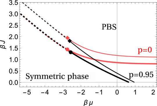
Figure 7: (Colour online) Phase diagram of the model on the Husimi lattice (thick curves) and on the Bethe lattice (thin curves) for two fixed values of the parameter $p$. Red curves correspond to $p=0$ (no repulsion between dissimilar species), while black curves - to $p=0.95$ (strong repulsion between dissimilar species). The solid curves are the lines of a continuous phase transition, while the dashed curves are the lines of a first order phase transition. Note that the lines for the first order phase transition are only slightly dependent on the actual value of $p$ in both cases. Lines of first order and second order phase transitions meet at tricritical points denoted by diamonds for Bethe lattice and circles for Husimi lattice.

In Fig. 7 we depict a phase diagram of the model on the Husimi tree (for comparison, we present it together with its counterpart obtained for the Bethe lattice, which permits us to draw some general conclusions) for two particular values ($p=0$ and $p=0.95$) of the mean concentration of the catalytic bonds. We observe that, in general, a transition into the phase with a broken symmetry for systems with the same $J$, (which sets the strength of interactions between similar species), and the same value of $p$, (which defines the strength of repulsive interactions between dissimilar species), occurs on the Husimi tree at lower values of the chemical potential than on the Bethe lattice. Such a behaviour may be apparently attributed to the fact that on the Husimi tree, due to its specific geometry, the system is more frustrated than on the Bethe lattice, such that it appears somewhat easier to break the symmetry between the species. Hence, not counter-intuitively, the onset of the critical behaviour is shifted towards smaller values of $\beta\mu$. Further on, we realise that the strength of repulsive interactions between dissimilar species, does not affect in any noticeable way the location of the line of critical points corresponding to the first order phase transition, both for the Husimi tree and for the Bethe lattice; indeed, we see that on the Husimi tree for $p=0$, when such repulsive interactions are completely absent, and for $p=0.95$, when such interactions are strong, the thick dashed curves in Fig. 7 almost overlap. The same happens in case of the Bethe lattice (see thin dashed curves in Fig. 7). On the contrary, the precise location of the line of critical points corresponding to the continuous transition is very much dependent on the value of $p$, for both the Husimi and the Bethe lattice. As a consequence, also the loci of the tricritical points depend on $p$.

It might be instructive to consider the phase diagram in more detail for a particular case. To this end, we again concentrate on the limit when $J=0$. Similarly to the behaviour on the Bethe lattice, here one has only a continuous transition between a symmetric disordered phase and a phase with a broken symmetry. The critical value $z_{c}$ of the activity at which such a transition takes place obeys the quadratic equation

$$z_{c}^{2}{+}\frac{4(4{-}3p)(4{-}5p)}{8(1{-}p)(4{-}5p(2{-}p))}z_{c}+\frac{32{-}25p}{8(1{-}p)(4{-}5p(2{-}p))}{=}0,$$ (26)

whose only real and positive root is given by:

$$z_{c}(p)=\dfrac{5\sqrt{p(2-p)}+15p+17}{20\left(p-\dfrac{\sqrt{5}-1}{\sqrt{5}}\right)\left(\dfrac{\sqrt{5}+1}{\sqrt{5}}-p\right)}\,.$$ (27)

As one can infer from equation (27), the critical value $z_{c}(p)$ of the activity is negative and therefore unphysical for $p$ below the critical value $p^{\rm(Hus)}=(\sqrt{5}-1)/\sqrt{5}\approx 0.553$. Therefore, for $p<p^{\rm(Hus)}$ the system does not undergo any phase transition. Note, that the phase with a broken symmetry may thus emerge on the Husimi lattice at smaller values of $p$ than in case of the Bethe lattice, because $p^{\rm(Hus)}<p^{\rm(Bet)}$.

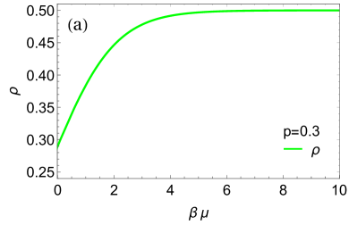
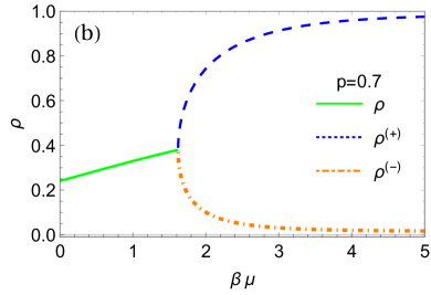
Figure 8: (Colour online) The Husimi lattice with $J=0$. The particles’ mean density as a function of $\beta\mu$ for two cases of the disordered degree: (a) $p=0.3<p^{\rm(Hus)}$, (b) $p=0.7>p^{\rm(Hus)}$. The green curves correspond to density $\rho=\rho^{(A)}=\rho^{(B)}$, blue and orange curves correspond to the particles mean densities in the phase with a broken symmetry, whose limiting values $\rho^{(+)}$ and $\rho^{(-)}$ are given in equations (4). The transitions from a symmetric phase into the phase with a broken symmetry occurs at the critical values of chemical potential defined in equation (27).

In Fig. 8 we depict the mean densities of the $A$ and $B$ particles as functions of $\beta\mu$ for two cases: $p<p^{\rm(Hus)}$ and $p>p^{\rm(Hus)}$. We observe that, in general, the behaviour is very similar to the one found in case of the Bethe lattice (see Fig. 4) and differs only in the loci of the critical points. Indeed, we see that for $p=0.3<p^{\rm(Hus)}$ both mean densities are equal to each other for any value of $\beta\mu$ and tend towards their limiting value $=1/2$ when the chemical potential tends to infinity. For $p=0.7>p^{\rm(Hus)}$, likewise it happens in case of the Bethe lattice (see Fig. 4b), the mean densities are equal to each other for sufficiently small values of $\beta\mu$ and then, at a certain value of the chemical potential, the symmetry is broken and one the species (which is equally probable for either $A$ or $B$) gets present in majority with the mean density $\rho^{(+)}$, while the second one becomes a minority component with the mean density $\rho^{(-)}$. In the limit $\beta\mu\to\infty$, the densities in the phase with a broken symmetry approach their limiting $p$-dependent values

$$\rho^{(+)}\Big{|}_{(\beta\mu)\to\infty} = \frac{1}{2}+\frac{\sqrt{p(2-p)\Big{(}5(2-p)p-4\Big{)}}}{2\Big{(}3(2-p)p-2\Big{)}},$$

$$\rho^{(-)}\Big{|}_{(\beta\mu)\to\infty} = \frac{1}{2}-\frac{\sqrt{p(2-p)\Big{(}5(2-p)p-4\Big{)}}}{2\Big{(}3(2-p)p-2\Big{)}},$$ (28)

which have a bit more complicated form than the ones found for the Bethe lattice (see equation (3.1)). Note that similarly to the behaviour on the Bethe lattice, a complete breaking of the symmetry occurs only for $p\equiv 1$, and in this case only $\rho^{(+)}=1$ and $\rho^{(-)}=0$. For any intermediate value of $p$ bounded away from $1$, both the majority and the minority components are present in the system. We also note parenthetically that, likewise as it was observed for the Bethe lattice, the values of the mean densities on the Husimi lattice are not very far from $1/3$ for zero chemical potential (see C). Lastly, in Fig. 5 we depict the order parameter $\Delta\rho$ for the model on the Husimi lattice, which is defined explicitly by (see B for the details of a derivation)

$$\Delta\rho=|\rho^{(A)}{-}\rho^{(B)}|=\frac{4zuv}{1+2z\left(u^{2}+v^{2}\right)}.$$ (29)

Note that $\Delta\rho$ is equal to zero ($v=0$) within the symmetric phase, and has a non-zero value within the phase with a broken symmetry. As one infers from Fig. 5, the order parameter on the Husimi lattice shows essentially the same behaviour as its counterpart for the Bethe lattice. The only differences are a) that the critical point on the Husimi lattice is shifted towards smaller values of the chemical potential, and b) that $\Delta\rho$ on the Husimi lattice attains substantially higher values for fixed $\beta\mu$ than its counterpart on the Bethe lattice, meaning that the effect of a broken symmetry is higher on the Husimi lattice than on the Bethe one.

Finally, we address a question whether on the Husimi lattice there exist phases with an alternating order, which we have observed for the Bethe lattice. As a matter of fact, here the situation appears to be quite delicate, as it was shown in Ref. [56]. The point is that for systems with repulsive inter-particle interactions (or antiferromagnetic interactions for spin models) defined on lattices with a geometrical frustration a robust analysis should be based from the very beginning on a description which involves all possible sub-lattices. In other words, in our case one has to consider simultaneously the recursions obeyed by the auxiliary partition functions on all three sub-lattices, i.e. we have to face six coupled non-linear equations instead of equations (4). In particular, such an approach is the only way to determine the antiferromagnetic phase transition on the square Husimi lattice [57]. In doing so, we have found by checking obtained equations numerically that for the case under study with $t=2$ the physically plausible expressions for the roots, that have to be real and positive, arise only when the auxiliary partition functions defined for different sub-lattices are equal to each other. Recall that an analogous observation was made for the antiferromagnetic spin-$1$ model defined on the Husimi lattice [51]. We therefore conclude that on the Husimi lattice with $t=2$ there is no alternating order phase. Of course, this does not rule out such a possibility for similarly constructed pseudo-lattices with $t\geq 3$. We note that it appears technically very difficult to tackle the systems with $t\geq 3$, in view of a strongly non-linear character of the recursion relations (4). Such an analysis will be presented elsewhere.

5 Conclusions

To recapitulate, we studied here thermodynamic equilibrium properties of a binary lattice-gas comprising interacting $A$ and $B$ particles, (or, in other words, a ternary mixture of two kinds of particles, and voids), which undergo continuous exchanges with their respective reservoirs, maintained at equal chemical potentials, $\mu_{A}=\mu_{B}=\mu$. Apart from the hard-core exclusion, particles of similar species experience nearest-neighbour interactions of amplitude $J$, which is the same for $AA$ and $BB$ pairs and may be positive or negative. In turn, neighbouring particles of dissimilar species repel each other, which represents a rather unusual physical situation. In our settings such a repulsion between dissimilar species emerges naturally within an analysis of the binary reactive lattice gases model in presence of special catalytic bonds, with random annealed spatial distribution and mean concentration $p$. As a consequence, the magnitude of the repulsion is controlled by $p$: $p=0$ corresponds to a zero repulsion, while $p=1$ – to an infinitely strong repulsion, when an $A$ and a $B$ cannot reside simultaneously on two neighbouring sites. For intermediate values of $p$, the repulsive interactions have a finite magnitude. Overall, our model is closely related to well-studied models of the so-called hard-objects on regular or pseudo-lattices.

For two kinds of standard pseudo-lattices - the Bethe lattice and the Husimi lattice - we determined the full phase diagram of such a lattice gas. We showed that the latter is rather complicated and contains several phases. More specifically, we demonstrated that there exists a phase with a spontaneously broken symmetry between $A$s and $Bs$, in which the species are present at two distinct mean densities, despite the fact that all the parameters are the same for both species. Further on, there is a symmetric phase, in which the species are present at equal mean densities. A transition from a symmetric phase into a phase with a broken symmetric may be of the first order or continuous. Such two phases exist on both the Bethe lattice and the Husimi lattice and only the precise location of the critical points is somewhat different; we realised that, in general, for the same $J$ and $p$, the symmetry is broken on the Husimi lattice at smaller values of the chemical potential than on the Bethe one.

Lastly, we showed that on the Bethe lattice there exist two phases with a structural order: in one of them the system spontaneously partitions into two sub-lattices one of which is occupied by both kinds of particles present with the same mean density, while the second sub-lattice is almost empty. In the second phase, the system again splits into two sub-lattices one of which is occupied by one kind of species, while the second sub-lattice is occupied by the other one. The system enters the first phase and leaves it via a continuous transition, and also enters the second phase via a continuous transition. Such phases are absent on the Husimi lattice due to stronger frustration effects.

Appendix A The Bethe lattice

A.1 Derivation of the recursion relations obeyed by $x_{N}$ and $y_{N}$.

We focus on the derivation of the recursion relations (3). To render our derivation more transparent, we let the activities of $A$ and $B$ particles be different, (denoting them as $z_{A}$ and $z_{B}$, respectively), and also let the amplitudes of the $A-A$ and $B-B$ interactions be different, $J_{A}$ and $J_{B}$. This will permit us to highlight different contributions in a more explicit way. Moreover, keeping the activities different will permit us to evaluate the mean densities of both species, by a mere differentiation of the free energy over the corresponding activity. In the final results, we will eventually return to the symmetric case.

The first step consists in considering three possible events with respect to the occupation of the root site $O$. The grand partition function (2) in this case can be written for $N$ generations of entire Cayley tree:

$$Z(p)=Z_{N}^{(0)}(p)+Z_{N}^{(A)}(p)+Z_{N}^{(B)}(p),$$ (30)

where $Z_{N}^{(0)}(p)$, $Z_{N}^{(A)}(p)$, $Z_{N}^{(B)}(p)$ are grand partition functions with vacant root site, occupied by an $A$ particle and occupied by a $B$ particle, respectively. The Cayley tree with the specified occupation of $O$ naturally decomposes into $q$ independent branches, each being a rooted tree with a prescribed occupation of the root site, which leads to our equation (4). We introduce then auxiliary functions $C_{N}(0,p)$, $C_{N}(A,p)$ and $C_{N}(B,p)$ through the relations :

$$Z_{N}^{(0)}(p)=C_{N}^{q}(0,p),\quad Z_{N}^{(A)}(p)=z_{A}^{1-q}C_{N}^{q}(A,p),\quad Z_{N}^{(B)}(p)=z_{B}^{1-q}C_{N}^{q}(B,p).$$ (31)

We note that each of the rooted trees contains $q-1$ identical sub-branches (which are also rooted trees) with $N$ generations. At the second step, we consider all possible values of the occupation variables of the sites neighbouring to the root. In doing so, we realise that the auxiliary functions in equation (31) obey

$$C_{N}(0,p) = C_{N-1}^{q-1}(0,p)+z_{A}^{2-q}C_{N-1}^{q-1}(A,p)+z_{B}^{2-q}C_{N-1}^{q-1}(B,p),$$

$$C_{N}(A,p) = z_{A}C_{N-1}^{q-1}(0,p)+z_{A}^{3-q}e^{\beta J_{A}}C_{N-1}^{q-1}(A,p)$$

$$+ (1-p)z_{A}z_{B}^{2-q}C_{N-1}^{q-1}(B,p),$$

$$C_{N}(B,p) = z_{B}C_{N-1}^{q-1}(0,p)+(1-p)z_{A}^{2-q}z_{B}C_{N-1}^{q-1}(A,p)$$ (32)

$$+ z_{B}^{3-q}e^{\beta J_{B}}C_{N-1}^{q-1}(B,p),$$

which permit us to eventually establish the desired recursion relations. The latter simplify once we introduce new variables $x_{N}$ and $y_{N}$, defined as the ratios of the auxiliary functions,

$$x_{N}=\frac{C_{N}(A,p)}{z_{A}C_{N}(0,p)},\qquad{\text{and}}\qquad y_{N}=\frac{C_{N}(B,p)}{z_{B}C_{N}(0,p)}.$$ (33)

In terms of $x_{N}$ and $y_{N}$, we get a system of two coupled non-linear recursion relations:

$$x_{N}=\frac{1+z_{A}e^{\beta J_{A}}x_{N-1}^{q-1}+(1-p)z_{B}y_{N-1}^{q-1}}{1+z_{A}x_{N-1}^{q-1}+z_{B}y_{N-1}^{q-1}},$$

$$y_{N}=\frac{1+(1-p)z_{A}x_{N-1}^{q-1}+z_{B}e^{\beta J_{B}}y_{N-1}^{q-1}}{1+z_{A}x_{N-1}^{q-1}+z_{B}y_{N-1}^{q-1}}.$$ (34)

In the symmetric case under study here, i.e. when $J_{A}=J_{B}=J$ and $z_{A}=z_{B}=z$, equations (A.1) reduce to our equations (3).

Mean densities of $A$ and $B$ species on the central site $O$ of the Cayley tree can be expressed in the following form

$$\rho_{0}^{(A)}{=}\frac{Z_{N}^{(A)}(p)}{Z_{N}^{(0)}(p){+}Z_{N}^{(A)}(p){+}Z_{N}^{(B)}(p)},\quad\rho_{0}^{(B)}{=}\frac{Z_{N}^{(B)}(p)}{Z_{N}^{(0)}(p){+}Z_{N}^{(A)}(p){+}Z_{N}^{(B)}(p)}.$$ (35)

Using (31) and (33) we get expressions in the variables $x_{N}$ and $y_{N}$:

$$\rho_{0}^{(A)}=\frac{z_{A}x_{N}^{q}}{1+z_{A}x_{N}^{q}+z_{B}y_{N}^{q}},\qquad\rho_{0}^{(B)}=\frac{z_{B}y_{N}^{q}}{1+z_{A}x_{N}^{q}+z_{B}y_{N}^{q}}.$$ (36)

A.2 Free energy of a binary mixture of particles on the Bethe lattice.

Derivation of the free energy of a binary lattice-gas of particles (a ternary mixture of particles and voids) on the Bethe lattice follows the general approach of Ref. [55], which applies to (rather) arbitrary recursive lattices. Substituting equations (31) into expression (4), we find that the free energy of a tree with $N$-generations obeys:

$$-\beta F_{N}=\ln Z_{N}=q\ln C_{N}(0,p)+\ln(1+z_{A}x_{N}^{q}+z_{B}y_{N}^{q}).$$ (37)

Taking the advantage of the recursions (A.1), we have then that

$$-\beta F_{N}=-(q-1)^{n}\beta F_{N-n}-\beta F_{Nn}\,,$$ (38)

where $F_{Nn}$ stands for the free energy of the model on a subtree with $n$ generations ($n\leq N$) within the Cayley tree with $N$ generations. The latter property is given by:

$$-\beta F_{Nn} {=}q\sum_{K=1}^{n}(q{-}1)^{K{-}1}\ln{\left(1{+}z_{A}x_{N{-}K}^{q{-}1}{+}z_{B}y_{N{-}K}^{q{-}1}\right)}$$

$${-}(q{-}1)^{n}\ln{\left(1{+}z_{A}x_{N{-}n}^{q}{+}z_{B}y_{N{-}n}^{q}\right)}{+}\ln{\left(1{+}z_{A}x_{N}^{q}{+}z_{B}y_{N}^{q}\right)}.$$ (39)

Further on, in the limit $N\to\infty$ (such that all $x_{N-K}\equiv x$ and $y_{N-K}\equiv y$) the resulting expression for $F_{n}$ attains the form

$$-\beta F_{n} = q\frac{(q-1)^{n}-1}{q-2}\ln(1+z_{A}x^{q-1}+z_{B}y^{q-1})$$ (40)

$$- ((q-1)^{n}-1)\ln(1+z_{A}x^{q}+z_{B}y^{q}).$$

The last step consists in turning to the limit of the so-called Bethe lattice - a deep interior of the Cayley tree far away from the boundary sites. Within this interior part, which is the Cayley tree with $n$ generations, all the bulk sites are considered to be equivalent. According to [13] (see also Refs. [58] and [55] for an additional discussion), the number $N^{B}_{s}$ of such sites is simply related to the number $N^{B}_{b}$ of bonds via the homogeneity assumption, $N^{B}_{b}/N^{B}_{s}=q/2$. For the Cayley tree with $n$ generations one has $N^{B}_{b}=q((q-1)^{n}-1)/(q-2)$. Therefore, the number of sites is given by $N^{B}_{s}=2((q-1)^{n}-1)/(q-2)$, such that we get:

$$-\beta f = -\frac{\beta F_{n}}{N^{B}_{s}}=\frac{q}{2}\ln(1+z_{A}x^{q-1}+z_{B}y^{q-1})$$ (41)

$$- \frac{q-2}{2}\ln(1+z_{A}x^{q}+z_{B}y^{q}).$$

This is the desired expression for the free energy on the Bethe lattice.

A.3 Fixed point solutions of recursions

Symmetric phase versus the phase with a broken symmetry. Let us suppose from now on that the strength of interactions between similar species is the same, i.e., $J_{A}=J_{B}=J$. Then, we assume that in the limit $N\to\infty$ the auxiliary variables $x_{N}\to x$ and $y_{N}\to y$, such that in this limit the system of equations (A.1) takes the form:

$$x=\tilde{g}(x,y),\qquad\tilde{g}(x,y)=\frac{1+e^{\beta J}\,z_{A}x^{q-1}+(1-p)z_{B}y^{q-1}}{1+z_{A}x^{q-1}+z_{B}y^{q-1}},$$ (42)

$$y=\tilde{h}(x,y),\qquad\tilde{h}(x,y)=\frac{1+(1-p)\,z_{A}x^{q-1}+e^{\beta J}z_{B}y^{q-1}}{1+z_{A}x^{q-1}+z_{B}y^{q-1}}.$$ (43)

Free energy per site of the Bethe lattice then obeys equation (41).

Since we consider an infinitely deep interior of the Cayley tree, in which all sites are equivalent, mean densities of both kinds of particles are defined by expressions (36),

$$\rho^{(A)}=\frac{z_{A}x^{q}}{1+z_{A}x^{q}+z_{B}y^{q}},\qquad\rho^{(B)}=\frac{z_{B}y^{q}}{1+z_{A}x^{q}+z_{B}y^{q}}.$$ (44)

Note that our equation (7) in the main text follows from the latter expression by setting $z_{A}=z_{B}=z$.

We thus now have all necessary ingredients for our analysis. Following Ref. [37], we first formally cast equations (42) and (43) into the form

$$z_{A}x^{q-1}=\frac{x(1-e^{\beta J})-py+p+e^{\beta J}-1}{(1-p-e^{\beta J})(1-p+e^{\beta J}-x-y)}$$ (45)

$$z_{B}y^{q-1}=\frac{y(1-e^{\beta J})-px+p+e^{\beta J}-1}{(1-p-e^{\beta J})(1-p+e^{\beta J}-x-y)}.$$ (46)

Next, introducing variables $u=(x+y)/2$ and $v=(x-y)/2$, we get two following equations

$$z_{A}z_{B}=\frac{((u-1)^{2}-\alpha^{2}v^{2})}{4(\gamma-u)^{2}(u^{2}-v^{2})^{q-1}},$$ (47)

$$z_{A}/z_{B}=\frac{(u-1+\alpha v)(u-v)^{q-1}}{(u-1-\alpha v)(u+v)^{q-1}},$$ (48)

where $\alpha$ and $\gamma$ are given by

$$\alpha=\frac{1-e^{\beta J}+p}{1-e^{\beta J}-p},\qquad\gamma=(1-p+e^{\beta J})/2\,.$$ (49)

Standard analysis (see Ref. [37] for more details), which we perform only for the symmetric case $z_{A}=z_{B}=z$, then shows that there are two different fixed point solutions corresponding to two stable thermodynamics phases:
(i) The solution with $v=0$ is given by

$$z=\frac{u-1}{2(\gamma-u)u^{q-1}},$$ (50)

which corresponds to a situation with equal mean densities of $A$ and $B$ species. This solution thus describes the disordered symmetric phase.
(ii) The solution with $v\neq 0$ is defined by the two following equations

$$\left\{\begin{array}[]{ c }(\alpha-(q-1)\frac{u-1}{u})+(C^{2}_{q-1}\alpha-C^{2}_{q-1}\frac{u-1}{u})\left(\frac{v}{u}\right)^{2}+\dots+\alpha\left(\frac{v}{u}\right)^{q-1}\\ \mbox{for}\quad q\quad\mbox{ odd}\\ (\alpha{-}(q{-1})\frac{u{-}1}{u}){+}(C^{2}_{q-1}\alpha{-}C^{2}_{q-1}\frac{u-1}{u})\left(\frac{v}{u}\right)^{2}{+}{\dots}{+}(\alpha(q-1){-}\frac{u-1}{u})\left(\frac{v}{u}\right)^{q-1}\\ \mbox{for}\quad q\quad\mbox{ even}\end{array}\right\}{=}0,$$ (55)

where $C^{k}_{n}$ stands for the binomial coefficient, and

$$z^{2}=\frac{(u-1)^{2}-\alpha^{2}v^{2}}{4(\gamma-u)^{2}(u^{2}-v^{2})^{q-1}}\,.$$ (57)

This solution defines the phase with a spontaneously broken symmetry between the species. Correspondingly, the demarkation surface between the symmetric phase and the phase with a broken symmetry in the region of continuous transitions obtains by substituting $v=0$ into the expressions (50), which yields $u_{c}=(q-1)/(q-1-\alpha)$ at the transition. Then substituting the latter expression for $u_{c}$ into equation (55) and setting $v=0$, we get

$$z_{c}=\frac{u_{c}-1}{2(\gamma-u_{c})u_{c}^{q-1}}.$$ (58)

In turn, the line of the trictitical points is obtained by using the condition

$$\frac{\delta z}{\delta u}\Big{|}_{v=0}=\frac{\partial z}{\partial u}\Big{|}_{v=0}+\frac{\partial z}{\partial v^{2}}\frac{\partial v^{2}}{\partial u}\Big{|}_{v=0}=0\,,$$ (59)

which is to be taken at $u=u_{c}$. Substituting equation (57) into condition (59), we get

$$\frac{(q-1)}{(\gamma-1)(q-1-\alpha)-\alpha}-q+2-\frac{(q-3)(q-1-\alpha)}{2q(q-1)}=0.$$ (60)

The line of first order phase transitions, which meets at the tricritical fixed point with the line of second order phase transitions, can be obtained by equating the free energies (see equation (41)) calculated for different phases.

Lastly, we note that the obtained expressions for the limiting values of auxiliary variables $x$ and $y$, together with the expressions (44) which defines the mean densities, permit us to introduce a natural order parameter $\Delta\rho=|\rho^{(A)}-\rho^{(B)}|$. The latter is given explicitly by

$$\Delta\rho=v\frac{u(1+\alpha)-1}{u(u-2)+\alpha v^{2}+\gamma}\,.$$ (61)

This parameter is exactly equal to zero within the random symmetric phase and is non-zero within the phase with a broken symmetry (see Fig. 5). In A.4 below, we analyse its behaviour for $\mu$ close to the critical value $\mu_{c}$ of the chemical potential.

Symmetric phase with a structural order. As we have already mentioned in the main text, equations describing the symmetric phase with an alternating order are obtained from the recursion scheme (A.1) by re-iterating it once more, in order to express $x_{N}$ and $y_{N}$ through $x_{N-2}$ and $y_{N-2}$, in which $N$ and $N-2$ have the same parity. Turning to the limit $N\to\infty$, we formally rewrite equations (42) and (43) as

$$x=\tilde{g}(\tilde{g}(x,y),\tilde{h}(x,y))\,,\quad y=\tilde{h}(\tilde{g}(x,y),\tilde{h}(x,y))\,.$$ (62)

We find then that for $q=3$, for some negative $J$ and for a certain interval of values of $p$ equations (62) possess three kinds of solutions with $x=y$ (or $v=0$):
– Solution $x_{odd}=x_{even}=y_{odd}=y_{even}$, equation (50), which corresponds to a situation with equal mean densities of $A$ and $B$ particles and no alternating order.
– Solution $x_{odd}=y_{odd}\neq x_{even}=y_{even}$ is one of the solutions of the following quadratic equation, obtained by re-iterating the recursion scheme,

$$u^{2}z\left(z\left(e^{J}-p+1\right)^{2}+2\right)+uz\left(e^{J}-p-1\right)+z\left(e^{J}-p+1\right)+1=0,\,\,\,u=(x+y)/2\,.$$ (63)

Note that here there is an alternating order, when the system spontaneously partitions into two different sub-lattices: $A$s and $B$s occupy predominantly one of them, while the second one is almost empty. This phase (PAO I) is defined by the following inequality

$$z\left(1+p-e^{\beta J}\right)^{2}-4\Big{(}z\left(1-p+e^{\beta J}\right)+1\Big{)}\left(z\left(1-p+e^{\beta J}\right)^{2}+2\right)\geq 0,$$ (64)

which gives, in turn, the condition that the solutions of equation (63) are real.
– Solution $x_{odd}=y_{even}\neq x_{even}=y_{odd}$. We find this solution from the following quadratic equation:

$$z\left(u_{1}^{2}+e^{2\beta J}\right)\left(e^{\beta J}+p-1\right)+\left(u_{1}-e^{\beta J}\right)\sqrt{z\left(e^{\beta J}+p-1\right)}\left(\left(u_{1}+p-1\right)\sqrt{z\left(e^{\beta J}+p-1\right)}\right.$$

$$-\left.\sqrt{z\left(e^{\beta J}-p+1\right)^{2}\left(e^{\beta J}+p-1\right)+4\left(e^{\beta J}-p-1\right)}\right)+2e^{\beta J}-2=0,$$ (65)

where $u_{1}=(x_{odd}+y_{even})/2$, $u_{2}=(x_{even}+y_{odd})/2$ and hence,

$$u_{2}^{2}=\frac{u_{1}-1+z\,u_{1}^{2}\left(u_{1}-1+p\right)}{z\left(e^{\beta J}-u_{1}\right)}.$$ (66)

Solutions of equations (A.3)) and (66) correspond to another kind of an alternating order, when the system spontaneously partitions into two different sub-lattices containing predominantly either kind of particles, i.e. $A$s and $B$s occupy predominantly different sub-lattices (PAO II). This phase is defined by the inequality:

$$4\,z\,(3e^{\beta J}+p-1)(e^{\beta J}+p-1)^{2}+(3e^{\beta J}+p-3)^{2}\geq 0.$$ (67)

A.4 Critical exponents

We focus here on the critical exponent describing scaling behaviour of the order parameter in the vicinity of a critical point. Following Ref. [37] let us denote

$$u-u_{c}=u_{c}\delta,\quad v=u_{c}\varepsilon,$$ (68)

where $u_{c}=(q-1)/(q-1-\alpha)$. Expanding the expressions (55) and (57) near the line of critical points, we obtain

$${h} {=\varepsilon\left[1-q+\alpha a+\left(q-1-\alpha a^{2}\right)\delta+\frac{1}{3}\left(1-q+\alpha^{3}a^{3}\right)\varepsilon^{2}+\left(1-q+\alpha a^{3}\right)\delta^{2}\right.}$$

$${\left.+\left(q-1-\alpha^{3}a^{4}\right)\delta\varepsilon^{2}+\frac{1}{5}\left(1-q+\alpha^{5}a^{5}\right)\varepsilon^{4}+\mathcal{O}\left(\varepsilon^{6},\varepsilon^{4}\delta,\varepsilon^{2}\delta^{2},\delta^{3}\right)\right]},$$ (69)

$$\mu-\mu_{c} =-\left(q-1-a-b\right)\delta+\frac{1}{2}\left(q-1-\alpha^{2}a^{2}\right)\varepsilon^{2}+\frac{1}{2}\left(q-1-a^{2}+b^{2}\right)\delta^{2}$$

$$-\left(q-1-\alpha^{2}a^{3}\right)\varepsilon^{2}\delta+\frac{1}{4}\left(q-1-\alpha^{4}a^{4}\right)\varepsilon^{4}+\mathcal{O}\left(\varepsilon^{6},\varepsilon^{4}\delta,\varepsilon^{2}\delta^{2},\delta^{3}\right),$$ (70)

where $h=(\mu_{A}-\mu_{B})/2$, $\mu=(\mu_{A}+\mu_{B})/2$, $\mu_{c}$ is defined in equation (58), while $a=u_{c}/(u_{c}-1)$ and $b=u_{c}/(\gamma-u_{c})$. Consequently, the behaviour of the order parameter (defined in equation (61)) in a vicinity of the critical point is given by

$$\Delta\rho=\frac{u_{c}\left[u_{c}(1+\alpha)-1\right]}{u_{c}(u_{c}-2)+\gamma}\varepsilon+\mathcal{O}\left(\delta,\varepsilon^{3}\right).$$ (71)

Next, using the condition $h=0$, we find that $\delta=\varepsilon^{2}(q-2)q(u_{c}-1)/3$ at the critical points, and hence, it follows from equation (A.4) that

$$\mu-\mu_{c}=\mu_{1}\Delta\rho^{2}+\mathcal{O}\left(\Delta\rho^{4}\right),$$ (72)

with

$$\mu_{1} =\frac{(q-2)}{3q^{2}}\frac{{u_{c}(u_{c}-2)+\gamma}}{(u_{c}-1)^{2}u_{c}^{3}}\left(\frac{(q-1)}{{(\gamma-1)}(q-1-\alpha)-\alpha}-q+2-\frac{(q-3)(q-1-\alpha)}{2q(q-1)}\right)$$ (73)

It follows thus that in the vicinity of a line of critical points a scaling behaviour of the order parameter is characterised by a classical mean-field critical exponent $\beta=1/2$ (i.e. $\Delta\rho\sim|\mu-\mu_{c}|^{\beta}$). This is not true, however, for the tricritical point at which $\mu_{1}$ vanishes, $\mu_{1}=0$. At the tricritical point the expansion (72) ensures that the tricritcal exponent $\beta_{2}=1/4$.

Appendix B The Husimi lattice

B.1 Recursions obeyed by $x_{N}$ and $y_{N}$.

The grand canonical partition function on the Husimi lattice with $N$ generations is first written in the same form as the one for the Bethe lattice (see equation (30)), by considering three possible events with respect to the occupation of the root site. Then, expressing the grand canonical partition functions of the rooted trees with a specified occupation of the root site $O$, i.e. $Z_{N}^{(0)}(p)$, $Z_{N}^{(A)}(p)$ and $Z_{N}^{(B)}(p)$, respectively, through the auxiliary functions $D_{N}(0,p)$, $D_{N}(A,p)$ and $D_{N}(B,p)$:

$$Z_{N}^{(0)}(p)=D_{N}^{t}(0,p),\quad Z_{N}^{(A)}(p)=z_{A}^{1-t}D_{N}^{t}(A,p),\quad Z_{N}^{(B)}(p)=z_{B}^{1-t}D_{N}^{t}(B,p)\,,$$ (74)

we find, following essentially the same procedure as in case of the Bethe lattice, that the functions $D_{N}$ obey recursions of the following form:

$$D_{N}(0,p) {=}D_{N-1}^{2(t-1)}(0,p){+}2z^{2-t}_{A}D_{N-1}^{t-1}(0,p)D_{N-1}^{t-1}(A,p)$$

$${+}2z^{2{-}t}_{B}D_{N{-}1}^{t{-}1}(0,p)D_{N{-}1}^{t{-}1}(B,p){+}2z^{2{-}t}_{A}z^{2{-}t}_{B}(1{-}p)D_{N-1}^{t-1}(A,p)D_{N-1}^{t-1}(B,p)$$

$${+}z^{2(2{-}t)}_{A}e^{\beta J_{A}}D_{N-1}^{2(t{-}1)}(A,p){+}z^{2(2{-}t)}_{B}e^{\beta J_{B}}D_{N-1}^{2(t{-}1)}(B,p),$$ (75)

$$D_{N}(A,p) =z_{A}D_{N-1}^{2(t-1)}(0,p){+}2z^{3-t}_{A}e^{\beta J_{A}}D_{N-1}^{t-1}(0,p)D_{N-1}^{t-1}(A,p)$$

$${+}2z_{A}z^{2{-}t}_{B}(1-p)D_{N{-}1}^{t{-}1}(0,p)D_{N{-}1}^{t{-}1}(B,p)$$

$${+}2z^{3{-}t}_{A}z^{2{-}t}_{B}(1{-}p)e^{\beta J_{A}}D_{N-1}^{t-1}(A,p)D_{N-1}^{t-1}(B,p)$$

$${+}z^{5{-}2t}_{A}e^{3\beta J_{A}}D_{N-1}^{2(t{-}1)}(A,p){+}z_{A}z^{2(2{-}t)}_{B}e^{\beta J_{B}}(1{-}p)^{2}D_{N-1}^{2(t{-}1)}(B,p).$$ (76)

An analogous expression for $D_{N}(B)$ obtains from equation (76) by a mere interchange of symbols $A\leftrightarrow B$.

B.2 Free energy and mean densities

Performing the same procedure as it was done in the A.2 for the Bethe lattice (see also Ref. [55]), we find that for the Husimi lattice with $n$ generations which are deeply inside the tree, the free energy obeys

$$-\beta F_{n} =t\frac{2^{n}(t-1)^{n}-1}{2(t-1)-1}\ln\left({1+2z_{A}x^{t-1}+2z_{B}y^{t-1}{+}2z_{A}z_{B}(1-p)x^{t-1}y^{t-1}}\right.$$

$$\left.{+z_{A}^{2}e^{\beta J_{A}}x^{2(t-1)}+z_{B}^{2}e^{\beta J_{B}}y^{2(t-1)}}\right)-\left(2^{n}(t-1)^{n}-1\right)\ln(1+z_{A}x^{t}+z_{B}y^{t}).$$ (77)

where $x$ and $y$ are the fixed point solution given by equation (19). According to Ref. [55], the free energy per site in the bulk of the Husimi tree obtains by dividing the expression (B.2) by the number of bulk sites $N^{H}_{s}$, which equals $3((t-1)^{n}2^{n}-1)/(2(t-1)-1)$. Hence, the free energy per site on the Husimi lattice is given by

$$\hskip 28.45274pt-\beta f =-\frac{\beta F_{n}}{N^{H}_{s}}=\frac{t}{3}\ln\left({1+2z_{A}x^{t-1}+2z_{B}y^{t-1}{+}2z_{A}z_{B}(1-p)x^{t-1}y^{t-1}}\right.$$

$$\left.{+z_{A}^{2}e^{\beta J_{A}}x^{2(t-1)}+z_{B}^{2}e^{\beta J_{B}}y^{2(t-1)}}\right)-\frac{2t-3}{3}\ln(1+z_{A}x^{t}+z_{B}y^{t}).$$ (78)

We restrict our analysis in the main text to a particular choice $t=2$. For such a choice the number ($N^{H}_{s}$) of bulk sites of the Husimi tree and the number ($N^{B}_{s}$) of bulk sites of the Cayley tree with $q=3$ obey $N^{B}_{s}/N^{H}_{s}=2/3$.

In turn, the mean densities of both kinds of particles at the root site are defined in the general form by equation (35). Then, using equations (74) and (19), we get the following expression

$$\rho_{0}^{(A)}=\frac{z_{A}x_{N}^{t}}{1+z_{A}x_{N}^{t}+z_{B}y_{N}^{t}},\qquad\rho_{0}^{(B)}=\frac{z_{B}y_{N}^{t}}{1+z_{A}x_{N}^{t}+z_{B}y_{N}^{t}}.$$ (79)

Correspondingly, turning to the fixed point solutions of the recursions, we have that the mean densities of the species on the Husimi lattice are given by

$$\rho^{(A)}=\frac{z_{A}x^{t}}{1+z_{A}x^{t}+z_{B}y^{t}},\qquad\rho^{(B)}=\frac{z_{B}y^{t}}{1+z_{A}x^{t}+z_{B}y^{t}}.$$ (80)

Similarly as in case of Bethe lattice we can define here an order parameter as the difference of $\rho^{(A)}$ and $\rho^{(B)}$: $\Delta\rho=|\rho^{(A)}-\rho^{(B)}|$. Using equation (80), we can find an explicit form of $\Delta\rho$ in the terms of symmetric variables $u=(x+y)/2$ and $v=(x-y)/2$. Finally, the difference of $\rho^{(A)}$ and $\rho^{(B)}$ is given by:

$$\Delta\rho=|\rho^{(A)}-\rho^{(B)}|=\frac{4zuv}{1+2z(u^{2}+v^{2})}.$$ (81)

B.3 The surface of critical points

In the main text we have shown that for $J>0$ there are two different kinds of fixed point solutions of the recursion relations (4), which correspond to the symmetric phase (see equation (22)) and the phase with a broken symmetry (see equations (23) and (24)), respectively. In order to evaluate the expression which defines implicitly the surface of critical points, we solve the system of equations (22) and (23). Omitting the intermediate steps, we present below such an equation for $t=2$, $J_{A}=J_{B}=J$ and $z_{A}=z_{B}=z$:

$$4z^{2}e^{8\beta J}\left(e^{\beta J}{-}1\right){+}4ze^{7\beta J}\Bigl{(}1{-}(1{-}p)(9{-}7p)z\Bigr{)}{-}e^{6\beta J}\Bigl{(}1{+}4(3{+}p)z{-}52(1{-}p)^{2}z^{2}\Bigr{)}$$

$${-}4ze^{5\beta J}\Bigl{(}8{-}10(2{-}p)p{+}(1{-}p)^{3}(15{-}11p)z\Bigr{)}{+}2e^{4\beta J}\Bigl{(}3{-}5(2{-}p)p{+}52z{-}4p\left(23{-}p(9{+}p)\right)z$$

$${-}78(1{-}p)^{4}z^{2}\Bigr{)}{-}4e^{3\beta J}\Bigl{(}1{-}5p{-}(1{-}p)^{2}\left(1{-}25(2{-}p)p\right)z{-}5(1{-}p)^{5}(5{+}p)z^{2}\Bigr{)}$$

$${-}e^{2\beta J}\Bigl{(}\left(3{-}5(2{-}p)p\right)^{2}{+}4(1{-}p)^{2}\left(55{-}121p{+}5p^{2}(13{-}3p)\right)z{+}20(1{-}p)^{6}z^{2}\Bigr{)}$$

$${+}4(1{-}p)e^{\beta J}\Bigl{(}3{-}22p{+}25p^{2}{+}54(1{-}p)^{3}z\Bigr{)}{-}4(1{-}p)^{2}\Bigl{(}1{-}8p{+}16z(1{-}p)^{2}\Bigr{)}=0.$$ (82)

Analysing equation (B.3), we infer that the continuous transition takes place for the following value of the activity $z$:

$$z_{c}=\exp{((\beta\mu)_{c})}=\frac{\mathcal{D}-c_{1}}{2c_{2}},$$ (83)

where $\mathcal{D}$, $c_{1}$ and $c_{2}$ are given by

$$\mathcal{D} =\Bigl{(}e^{6\beta J}{+}e^{2\beta J}(1{-}p)\left(6e^{\beta J}{+}15{-}33p{+}5(3{-}p)p^{2}\right){-}2e^{4\beta J}\left(4{-}3(2{-}p)p\right)$$

$$+2(1{-}p)^{3}(4{-}11e^{\beta J})\Bigr{)}\Bigl{(}e^{3\beta J}+(4-5e^{\beta J})(1-p)^{2}\Bigr{)}^{1/2},$$

$$c_{1} =e^{6\beta J}\left(e^{\beta J}{-}3{-}p\right){-}2e^{5\beta J}\Bigl{(}4{-}5(2{-}p)p\Bigr{)}{-}2e^{4\beta J}(1{-}p)\Bigl{(}13{-}(10{+}p)p\Bigr{)}$$

$${+}e^{2\beta J}(1{-}p)^{2}\left(e^{\beta J}\Bigl{(}1{-}25(2{-}p)p\Bigr{)}{-}\Bigl{(}55{-}\Bigl{(}121{-}5p(13{-}3p)p\Bigr{)}\Bigr{)}{-}2(1{-}p)^{4}\left(8{-}27e^{\beta J}\right)\right),$$

$$c_{2} =e^{2\beta J}\Bigl{(}e^{2\beta J}{-}5(1{-}p)^{2}\Bigr{)}\left(e^{\beta J}{-}1{+}p\right)^{2}\Bigl{(}e^{2\beta J}\left(e^{\beta J}{+}1{-}2p\right){-}e^{\beta J}(1{-}p)(3{+}p){+}(1{-}p)^{2}\Bigr{)}.$$

Equating $c_{2}$ to zero, which enter equation (83), we readily find the threshold value $J(p)$ in equation (25).

B.4 Line of tricritical points

Here we present the exact equation, defining implicitly the line of tricritical points (see Fig. 7) on the Husimi lattice, which is obtained exactly along the same lines as in case of the Bethe lattice (see the A). For the Husimi lattice it has a rather complicated form :

$$e^{12(\beta J)_{tc}}{+}4e^{11(\beta J)_{tc}}(1{-}p){-}4e^{10(\beta J)_{tc}}\Bigl{(}6{-}(2{-}p)p\Bigr{)}{-}4e^{9(\beta J)_{tc}}(1{-}p)\Bigl{(}26{-}9(2{-}p)p\Bigr{)}$$

$${+}2e^{8(\beta J)_{tc}}\Bigl{(}71{-}16p{-}\left(56{-}17(4{-}p)p\right)p^{2}\Bigr{)}{+}4e^{7(\beta J)_{tc}}\Bigl{(}168{-}474p{+}511p^{2}{-}\left(281{-}15(5{-}p)p\right)p^{3}\Bigr{)}$$

$$-4e^{6(\beta J)_{tc}}(1-p)\Bigl{(}145+113p-477p^{2}+5\left(83{-}7(5{-}p)p\right)p^{3}\Bigr{)}$$

$$-4e^{5(\beta J)_{tc}}(1-p)^{2}\Bigl{(}446-936p+383p^{2}+\left(39-25(5-p)p\right)p^{3}\Bigr{)}$$

$$+e^{4(\beta J)_{tc}}(1-p)^{2}\Bigl{(}1785-78p-4357p^{2}+3308p^{3}-25\left(29+(6-p)p\right)p^{4}\Bigr{)}$$

$$+4e^{3(\beta J)_{tc}}(1-p)^{3}\Bigl{(}391-1264p+556p^{2}+5\left(44-19p\right)p^{3}\Bigr{)}$$

$${-}4e^{2(\beta J)_{tc}}(1{-}p)^{4}\Bigl{(}603{-}170p{-}\left(517{-}52p\right)p^{2}\Bigr{)}{+}16(1{-}p)^{5}\Bigl{(}14e^{(\beta J)_{tc}}(3{+}5p){+}4(1{-}p)\Bigr{)}{=}0.$$ (84)

Appendix C Mean densities at zero chemical potential and $J=0$

C.1 The mean particles’ densities on the Bethe lattice at $\mu=0$ and $J=0$.

In virtue of equation (44), the mean densities of particles of both kinds at zero chemical potential and at zero interaction strength $J$ obey

$$\rho=\rho_{A}=\rho_{B}=\frac{x^{q}}{1+2\,x^{q}},$$ (85)

where $x$ satisfies the equation

$$(x-1)(1+2x^{q-1})+p\,x^{q-1}=0.$$ (86)

For $p=0$, (i.e., no other interactions between the dissimilar species apart from the hard-core ones), the only real positive solution of equation (86) with arbitrary $q$ is $x\equiv 1$. In consequence, equation (85) entails $\rho\equiv 1/3$. This result is obvious, since in this case we have a three-state model without interactions and external fields; therefore, each of the species as well as the vacant sites are present at equal mean densities.

For $p\not=0$, the solution of equation (86) depends on both $q$ and $p$, and the mean density defined by equation (85) is evidently a decreasing function of these parameters. In Fig. 4 (a), for $q=3$ we have chosen $p=0.3$, and thus we find that the density at $\mu=0$ and $J=0$ is $\rho\approx 0.2993$, while for $p=0.7$ in Fig. 4 (b) the density at $\mu=0$ and $J=0$ is $\rho\approx 0.2543$.

C.2 The mean particles’ densities on the Husimi lattice at $\mu=0$ and $J=0$.

Similarly, on the Husimi lattice the mean particles’ densities for $\mu=0$ and $J=0$ obey

$$\rho=\rho_{A}=\rho_{B}=\frac{x^{t}}{1+2\,x^{t}},$$ (87)

where $x$ satisfies the equation

$$(x-1)\left(1+4x^{t-1}(1+x^{t-1})\right)+p\,x^{t-1}\left(2+(4-3p)x^{t-1}\right)=0.$$ (88)

For $p=0$, the only real positive solution of equation (88) is $x\equiv 1$ for arbitrary $t$, which again entails a trivial result $\rho\equiv 1/3$. For $p\not=0$, the mean density $\rho$ is again a decreasing function of the parameters $p$ and $t$. In Fig. 8 (a), for $t=2$ we have chosen $p=0.3$, and thus we find that the density at $\mu=0$ and $J=0$ is $\rho\approx 0.2922$, while for $p=0.7$ in Fig. 8 (b) the density at $\mu=0$ and $J=0$ is $\rho\approx 0.2529$, which is somewhat greater than the corresponding value of the mean density on the Bethe lattice.

References

References

- [1] Domb C 1958 Some Theoretical Aspects of Melting Nuovo Cimento 9 9
- [2] Rushbrooke GS and Scoins HI 1962 Cluster Sums for the Ising Model J. Math. Phys. 3 176
- [3] Gaunt DS and Fisher ME (1965) Hard-Sphere Lattice Gases. I. Plane-Square Lattice J. Chem. Phys. 43 2840
- [4] Baxter RJ, Enting IG and Tsang SK 1980 Hard-square lattice gas J. Stat. Phys. 22 465
- [5] Poland D 1984 On the universality of the non-phase transition singularity in hard-particle systems J. Stat. Phys. 35 341
- [6] Guttmann A J 1987 Comment on ”The exact location of partition function zeros, a new method for statistical mechanics” J. Phys. A: Math. Gen. 20 511
- [7] Lai S-N and Fisher ME 1995 The universal repulsive-core singularity and Yang-Lee edge criticality J. Chem. Phys. 103 8144
- [8] Todo S 1999 Transfer-matrix study of negative fugacity singularity of hard-core lattice gas Int. J. Mod. Phys. C 10 517
- [9] Temperley HNV 1965 An exactly soluble lattice model of the fluid-solid transition Proc. Phys. Soc. (London) 86 185
- [10] Burley DM 1960 A Lattice Model of a Classical Hard Sphere Gas Proc. Phys. Soc. London 75 262; 1961 A Lattice Model of a Classical Hard Sphere Gas: II, ibid 77 451
- [11] Runnels LK 1967 Phase transition of a Bethe lattice gas of hard molecules J. Math. Phys. 8 2081
- [12] Baxter RJ 1980 Hard hexagons: exact solution J Phys. A: Math. Gen. 13 L61
- [13] Baxter RJ 1982 Exactly Solved Models in Statistical Mechanics (Academic Press)
- [14] Bouttier J, Di Francesco P and Guitter E 2002 Critical and tricritical hard objects on bicolourable random lattices: exact solutions J. Phys. A: Math. Gen. 35 3821
- [15] Oliveira TJ and Stilck JF 2011 Solution on the Bethe lattice of a hard core athermal gas with two kinds of particles J. Chem. Phys. 135 184502
- [16] Ziff RM, Gulari E and Barshad Y 1986 Kinetic Phase Transitions in an Irreversible Surface-Reaction Model Phys. Rev. Lett. 56 2553
- [17] Marro J and Dickman R 1999 Nonequilibrium Phase Transitions in Lattice Models (Cambridge: Cambridge University Press)
- [18] Liu D-J and Evans J W 2013 Realistic multisite lattice-gas modeling and KMC simulation of catalytic surface reactions: Kinetics and multiscale spatial behavior for CO-oxidation on metal (1 0 0) surfaces Prog. Surf. Sci. 88 393
- [19] Oshanin G and Blumen A 1998 Kinetic description of diffusion-limited reactions in random catalytic media J. Chem. Phys. 108 1140
- [20] Toxvaerd S 1998 Molecular dynamics simulation of diffusion-limited catalytic reactions J. Chem. Phys. 109 8527
- [21] Argyrakis P, Burlatsky SF, Clément E and Oshanin G 2001 Influence of auto-organization and fluctuations on the kinetics of a monomer-monomer catalytic scheme Phys. Rev. E 63 021110
- [22] Coppey M, Bénichou O, Klafter J, Moreau M and Oshanin G 2004 Catalytic reactions with bulk-mediated excursions: Mixing fails to restore chemical equilibrium Phys. Rev. E 69 036115
- [23] Oshanin G and Burlatsky SF 2002 Single-species reactions on a random catalytic chain J. Phys. A: Math. Gen. 35 L695
- [24] Oshanin G, Bénichou O and Blumen A 2003 Exactly solvable model of reactions on a heterogeneous catalytic chain Europhys. Lett. 62 69
- [25] Oshanin G, Bénichou O and Blumen A 2003 Exactly Solvable Model of Reactions on a Random Catalytic Chain J. Stat. Phys. 112 541
- [26] Oshanin G and Burlatsky SF 2003 Adsorption of reactive particles on a random catalytic chain: An exact solution Phys. Rev. E 67 016115
- [27] Shapoval D, Dudka M, Bénichou O and Oshanin G 2020 Equilibrium properties of two-species reactive lattice gases on random catalytic chains Phys. Rev. E 102 032121
- [28] Dudka M, Bénichou O and Oshanin G 2018 Order-disorder transitions in lattice gases with annealed reactive constraints J. Stat. Mech. 2018 043206
- [29] Oshanin G, Popescu MN and Dietrich S 2004 Exactly Solvable Model of Monomer-Monomer Reactions on a Two-Dimensional Random Catalytic Substrate Phys. Rev. Lett. 93 020602
- [30] Popescu MN, Dietrich S and Oshanin G 2007 Binary reactive adsorbate on a random catalytic substrate J. Phys.: Condens. Matter 19 065126
- [31] Horiguchi T 1986 A spin-one Ising model on a honeycomb lattice Phys. Lett. A 113 425; Wu FY 1986 On Horiguchi’s solution of the Blume-Emery-Griffiths model Phys. Lett. A 116 245
- [32] Blume M, Emery V J, and Griffiths R B 1974 Ising Model for the Transition and Phase Separation in He3-He4 Mixtures Phys. Rev. A 4, 1071
- [33] Mukamel D and Blume M 1974 Ising model for tricritical points in ternary mixtures Phys. Rev. A 10 610
- [34] Prasad V V, Campa A, Mukamel D, and Ruffo S 2019 Ensemble inequivalence in the Blume-Emery-Griffiths model near a fourth-order critical point Phys. Rev. E 100, 052135
- [35] Harary F and Uhlenbeck GE 1953 On the number of husimi trees, Proc. Natl. Acad. Sci. USA 39 315
- [36] Pretti M 2003 A note on cactus trees: Variational vs. recursive approach, J. Stat. Phys. 111 993
- [37] Ananikian N S, Avakian A R and Izmailian N S 1991 Phase diagrams and tricritical effects in the beg model Physica A 172 391 (1991); https://doi.org/10.1016/0378-4371(91)90391-O Hu Ch-K and Izmailian N Sh 1998 Exact correlation functions of Bethe lattice spin models in external magnetic fields Phys. Rev. E 58 1644; https://doi.org/10.1103/PhysRevE.58.1644
- [38] Vannimenus J 1981 Modulated phase of an ising system with competing interactions on a Cayley tree Z. Phys. B 43 141.
- [39] Ananikian N, Izmailyan NS, Johnston D, Kenna R and Ranasinghe PKCM 2013 Potts models with invisible states on general Bethe lattices J. Phys. A: Math. Theor. 46 385002
- [40] Rivoire O, Biroli G, Martin OC and Mezard M 2004 Glass models on Bethe lattices Eur. Phys. J. B 37 55
- [41] De Luca A, Altshuler BL, Kravtsov VE and Scardicchio A 2014 Anderson Localization on the Bethe Lattice: Nonergodicity of Extended States Phys. Rev. Lett. 113 046806
- [42] Dudka M, Kondrat S, Kornyshev AA and Oshanin G 2016 Phase behaviour and structure of a superionic liquid in nonpolarized nanoconfinement J. Phys.: Condens. Matter 28 464007
- [43] Dudka M, Kondrat S, Bénichou O, Kornyshev AA and Oshanin G 2019 Superionic liquids in conducting nanoslits: A variety of phase transitions and ensuing charging behavior J. Chem. Phys. 151 184105
- [44] Majumdar SN and Privman V 1993 Journal of Physics A: Mathematical and General Annihilation of immobile reactants on the Bethe lattice J. Phys. A Math. Gen. 26, L743
- [45] Abad E 2004 On-lattice coalescence and annihilation of immobile reactants in loopless lattices and beyond Phys. Rev. E 70, 031110
- [46] Shapoval D, Dudka M, Durang X and Henkel M 2018 Crossover between diffusion-limited and reaction-limited regimes in the coagulation-diffusion process,Journal of Physics A: Mathematical and General 51, 425002; https://doi.org/10.1088/1751-8121/aadd53
- [47] Chatelain C, Henkel M, de Oliveira MJ and Tomé T 2012 Relaxation at finite temperature in Fully-Frustrated Ising Models J. Stat. Mech. P11006
- [48] Henkel M and Seno F 1996 Phase diagram of branched polymer collapse Phys. Rev. E 53 3662
- [49] de los Rios P, Lise S and Pelizzola A 2001 Bethe approximation for self-interacting lattice trees Europhys. Lett. 53 176
- [50] Groda Ya, Dudka M, Kornyshev AA, Oshanin G and Kondrat S 2021 Superionic liquids in conducting nanoslits: insights from theory and simulations J. Phys. Chem. C 125 9, 4968
- [51] Jurčišinová E and Jurčišin M 2016 Geometric frustration effects in the spin-1 antiferromagnetic Ising model on the kagome-like recursive lattice: exact results J. Stat. Mech. 093207; https://doi.org/10.1088/1742-5468/2016/09/093207
- [52] Jabar E and Masrour R 2018 Magnetic properties of simplest Husimi lattice: a Monte Carlo study J. Supercond. Nov. Magn. 31 4185; https://doi.org/10.1007/s10948-018-4705-9
- [53] Liao H J et al 2016 Heisenberg antiferromagnet on the Husimi lattice Phys. Rev. B 93 075154; https://doi.org/10.1103/PhysRevB.93.075154
- [54] Jurčišinová E, Jurčišin M and Bobák A 2014 The Exact Solution of the Anti-ferromagnetic Ising Model with Multisite Interaction on the Simplest Pure Husimi Lattice J. Stat. Phys. 154 1096
- [55] Ananikian NS, Izmailian NS and Oganessyan KA 1998 An Ising spin-S model on generalized recursive lattice Physica A 254 207
- [56] Monroe JL 1998 Frustrated Ising systems on Husimi trees Physica A 256 217; https://doi.org/10.1016/S0378-4371(98)00216-7
- [57] Huang R and Chen Ch 2014 Thermodynamic transition of antiferromagnetic Ising model on the fractional multi-branched Husimi recursive lattice Commun Theor. Phys 62 749; https://doi.org/10.1088/0253-6102/62/5/19
- [58] Gujrati PD 1995 Bethe or Bethe-like Lattice Calculations Are More Reliable Than Conventional Mean-Field Calculations Phys. Rev. Lett. 74 809