Slippery-Sticky Transition of Interfacial Fluid Slip

Abstract

The influence of temperature on interfacial fluid slip, as measured by molecular-dynamics simulations of a Couette flow comprising a Lennard-Jones fluid and rigid crystalline walls, is examined as a function of the fluid-solid interaction strength. Two different types of thermal behavior are observed, namely, the slippery and sticky cases. The first is characterized by a steep and unlimited increase of the slip length at low temperatures, while the second presents a vanishing slip length in this regime. As the temperature increases in relation to a characteristic value, both cases converge to finite slip lengths. A recently proposed analytical model is found to well describe both thermal behaviors, also predicting the slippery-sticky transition that occurs at a critical value of the fluid-solid interaction parameter, for which, according to the model, fluid particles experience a smooth average energy landscape at the interface.

I Introduction

Fluid-solid interaction is a fundamental topic in several areas of science and engineering.[1, 2, 3] Even more than this, almost every aspect of our daily lives is permeated by interfacial phenomena.[4] For this reason, an accurate description of fluid-solid interfaces is an invaluable tool in developing relevant scientific models and impactful technologies.

The purpose of this work is to examine the interfacial phenomenon of fluid slip.[5] This physical effect, quantified by the parameter known as slip length, is usually neglected in macroscopic-scale fluid models and simulations when specifying velocity-field boundary conditions. Due to the slip length’s typically small magnitude, often of the order of a few molecular diameters, the no-slip condition[6, 7] is generally used as a suitable approximation for the fluid tangential velocity at a solid surface for most common applications.[8, 9]

However, the no-slip condition does have its shortcomings. In particular, for small-scale flows, such as those in micropores and nanotubes, the no-slip condition leads to significant errors in the fluid velocity field and, as a consequence, incorrect flow rates are obtained, sometimes underestimating observed values by several orders of magnitude.[10, 11, 12] Furthermore, an intrinsic limitation of the no-slip condition is that it is indifferent to changes in the interface materials since it is entirely independent of the molecular structure, atomic composition, and thermodynamic state of either fluid or solid surface. This disagrees with empirical data and prevents the use of theoretical models and numerical simulations in the design, development, or selection of functional interfaces for target applications.

Although the conventional theoretical framework of fluid mechanics, which relies on the continuum hypothesis, is unable to determine interfacial boundary conditions, they can be readily assessed by employing atomistic simulation methods, such as molecular dynamics.[13, 14] Moreover, in this way, material-specific values of slip length can be computed for the system at hand and, additionally, their many parametric dependencies can be comprehensively analyzed.

Over the past few decades, plenty of effort has been directed towards understanding the mechanisms underlying fluid slip and the way it correlates with other physical quantities and phenomena.[15] In this regard, molecular-dynamics simulations have been employed in the investigation of fluid-slip processes[16, 17, 18, 19, 20, 21, 22] and their connection with shear rate,[23, 24] channel size,[25, 26] flow type,[27, 28] wall stiffness,[29, 30, 31, 32] thermodynamic variables,[33, 34, 35] wettability,[36, 37, 38, 39, 40, 41, 42, 43, 44, 45, 46, 47] interatomic interactions,[48, 49, 50, 51] as well as surface patterning and roughness.[52, 53, 54, 55, 56, 57, 58, 59]

The present work particularly addresses the functional relationship between slip length and temperature. More specifically, we build upon the study carried out by Wang and Hadjiconstantinou,[60] where a reaction-rate model describing fluid slip as a thermally-activated process was proposed. With the aid of non-equilibrium molecular-dynamics simulations, we evaluate the temperature dependence of slip length, as a function of the fluid-solid interaction strength, for an interface model consisting of a Lennard-Jones fluid and rigid walls. In this way, two completely opposite situations are observed, which we designate as slippery and sticky cases. The thermal-activation model is found to correctly describe both situations and precisely identify the interaction-parameter value at which the transition between them occurs. As shown in later sections, temperature is indeed a very influential variable on the slip-length value, with the ability to greatly amplify or suppress the fluid slip in the slippery and sticky cases, respectively.

The fundamental concepts and basic procedures employed in our numerical simulations and data analysis are briefly outlined in section II. Section III presents our main results, namely, an atomistic investigation of the fluid-slip thermal behavior for model interfaces. Further discussion on the results, based on the physical interpretation provided by the thermal-activation analytical model, is given in section IV. Section V comprises our concluding remarks and perspectives for future work. Details of the simulation setup are found in appendix A.

II Methodology

II.1 Slip Length

The slip length, denoted here by $\lambda$, is the parameter that quantifies the fluid slip at a point $\vec{r}$ of a solid surface $\mathcal{S}$ by relating the fluid-velocity tangential component $u_{t}$, in the rest frame of $\mathcal{S}$, to the local shear rate $\dot{\gamma}=\partial u_{t}/\partial n$, that is,

$$\left.u_{t}\right|_{\vec{r}\in\mathcal{S}}=\lambda\left.\frac{\partial u_{t}}{\partial n}\right|_{\vec{r}\in\mathcal{S}},$$ (1)

where $n$ is the direction of the surface’s normal pointing into the fluid. Geometrically, $\lambda$ is the distance one would have to linearly extrapolate the fluid velocity towards the solid surface so that $u_{t}$ vanishes.

It is important to note that equation (1) is composed of effective quantities, that is, both $u_{t}$ and its normal derivative must be understood as resulting from an extrapolation of the velocity field from some point sufficiently far into the fluid so that interfacial atomic-scale effects are not considered when evaluating $\lambda$. As a consequence, the slip length constitutes an apparent quantity, whose value directly corresponds to the expected observation of a fluid-solid interface in a continuum-fluid perspective.

The applicability of definition (1) is twofold. In an atomistic simulation, as in the case of the results discussed in later sections, equation (1) is the working formula used to compute the slip length from statistically-evaluated fluid velocity fields. On the other hand, in the context of continuum fluid dynamics, expression (1) becomes a third-type boundary condition, which can be used for solving the velocity field at fluid-solid interfaces, once slip-length values obtained by other means are provided.

II.2 Simulations

The adopted interface model consists of a monoatomic fluid bounded by two solid walls whose atoms are kept in a rigid simple-cubic crystal arrangement. Fluid particles have mass $m$ and both fluid-fluid and fluid-solid interactions are described by a pairwise Lennard-Jones potential,

$$V(r)=4\varepsilon\left[\left(\frac{\sigma}{r}\right)^{12}-\left(\frac{\sigma}{r}\right)^{6}\right],$$ (2)

where $r$ is the distance between interacting particles. The parameter $\varepsilon$ controls the strength of the interaction, while $\sigma$ sets its length scale. For computational reasons, interactions are turned off for distances larger than a cutoff radius $r_{c}$, so that forces are actually derived from a truncated and smoothed version of the potential, $\tilde{V}(r)=V(r)-V(r_{c})-\left.\partial{V(r)}/\partial{r}\right|_{r=r_{c}}(r-r_{c})$, thus ensuring the continuity of both energy and force at $r=r_{c}$.

Throughout this work, the values of $\sigma$ and $\varepsilon$ determining the fluid-fluid interaction are considered, respectively, as the length and energy units. That is, a Lennard-Jones system of units is here employed with the parameters of the fluid-fluid potential set as reference. As a result, the temperature unit becomes $\varepsilon/k_{B}$, where $k_{B}$ is the Boltzmann constant. In addition, by taking the mass $m$ of a fluid particle as the unit of mass, it follows that the unit of time is $\tau=\sigma\sqrt{m/\varepsilon}$. Note that, as a consequence of the adopted unit system, the Lennard-Jones parameters of the fluid-solid interaction, symbolized by $\varepsilon_{fs}$ and $\sigma_{fs}$, have their values specified in relation to the fluid-fluid potential.

In order to extract slip-length values from an interface model, the fluid must be put in a shearing state. For this purpose, a non-equilibrium methodology based on a molecular-dynamics Couette flow is employed. The simulation box is made periodic in the $x$ and $y$ directions while solid walls constrain the fluid in the $z$ dimension. The walls, symmetrical and placed a distance $h$ apart, move rigidly and uniformly in opposite directions along the $x$ direction with relative speed $U$. In addition, the walls are made thick enough so that fluid particles are unaware of the solid’s finite depth. After a transient period in its time evolution, the system reaches a steady state, which is characterized by a linear velocity profile $u_{x}(z)$ in the fluid’s bulk region, that is, in the volume portion sufficiently far from the solid walls. At this stage, the fluid also displays uniform bulk temperature and density profiles.

After ensuring that the system is in its steady state, the simulation enters in the production stage, in which velocities are sampled and averaged over several time steps. Once enough data is accumulated, the shear rate $\dot{\gamma}$ is evaluated by applying a linear regression to the resulting bulk velocity profile. Finally, the slip length is obtained from equation (1), which yields the relation $\lambda=(U/\dot{\gamma}-h)/2$ in the case of a Couette flow.

All simulation runs are performed using the same number of particles and box dimensions. In particular, the wall separation distance $h$ is kept constant so that the overall fluid density is fixed. However, as the fluid-solid interaction strength varies across runs, the layering effects at the interface cause slight variations in the bulk density. These deviations are very small, though, and do not noticeably affect the fluid slip. Also, it should be mentioned that, since slip-length values are presumably connected with continuum boundary conditions, it is important to consider a sufficiently large simulation box, so that confinement effects, which would be spurious in this context, are avoided. Preliminary simulations have been performed in order to determine suitable box dimensions, for which the fluid slip is nearly invariant against further increases in the system size.

For the purposes of the intended analysis, each slip-length value must be determined at a well-defined temperature. Since the wall motion gives rise to a net inflow of energy, it is crucial to take measures to keep the temperature at a constant average value. Following previous works,[23, 32] a Langevin thermostat is applied to fluid particles. This procedure amounts to adding a combination of stochastic and dissipative forces to the system dynamics. Given that $\vec{f}$ is the resultant conservative force acting on a fluid particle of acceleration $\vec{a}$, velocity $\vec{v}$, and position $\vec{r}$, the thermostatted equations of motion read

$$m\vec{a}=\vec{f}+\left\{-m\Gamma\left[\vec{v}-\vec{u}(\vec{r})\right]_{y}+S\right\}\hat{y},$$ (3)

where $\vec{u}$ is the fluid velocity field, $\Gamma$ is an adjustable damping coefficient, and $S(t)$ corresponds to a stochastic force satisfying $\langle S(t)\rangle=0$ and $\langle S(t)S(t^{\prime})\rangle=2mT_{b}\Gamma\delta(t-t^{\prime})$, with angle brackets denoting time averages. The imposed dynamics drive the system in such a way as to match the average fluid temperature $T$ to the target value $T_{b}$, representing the thermal-bath temperature. As shown in equation (3), only the particle acceleration in the $y$ direction is directly affected by ‘external’ nonconservative forces. This is so in order to minimize the influence of the thermostat on the $x$ and $z$ directions, which are actually relevant to the Couette flow, thus reducing the effects of forces extraneous to the shear dynamics on the measured velocity profile.

In all performed simulations, the Langevin thermostat was able to adequately control the fluid’s temperature, keeping its value spatially uniform and very close, except for temporal fluctuations, to the thermal bath’s temperature (see the inset of figure 1). In accordance, from now on, the symbol $T$ is used here to denote the time-averaged temperature of the fluid, whose value is virtually identical to the target parameter $T_{b}$.

According to previous studies,[62, 63, 64, 65] a low-density Lennard-Jones substance in thermodynamic equilibrium has a freezing temperature close to $0.69\varepsilon/k_{B}$. However, in the case of a non-equilibrium system, such as a Couette flow, the substance can still present fluidic behavior at lower temperatures. Moreover, the actual freezing temperature $T_{F}$ of a shearing fluid depends on its strength of interaction with the moving walls, as higher values of the parameter $\varepsilon_{fs}$ facilitate the system’s nucleation at the solid surfaces. For this reason, the temperature range used in our molecular-dynamics simulations differs for each choice of $\varepsilon_{fs}$, starting at the lowest temperature for which the Lennard-Jones substance properly displays a symmetrical Couette-flow pattern and going up to sufficiently high temperatures, where the slip-length variation is slow.

A point deserving closer examination is the fact that, in the adopted methodology, the walls move rigidly, meaning that solid particles do not respond to the forces acting upon them. This is done mainly for practical reasons, since it makes simulations simpler to implement and computationally cheaper. Hence, solid-solid interactions play no role and, in particular, temperature effects on the walls are disregarded. The question then arises whether this simplification significantly affects the slip length’s temperature dependence. A justification for the performed simulations can be found in previous studies,[32] which have shown that, at least for simple wall models with sufficiently high stiffness, variations in the interaction strength between solid-surface particles have little impact on the slip length, provided the fluid temperature is properly kept constant.

Additional technical details of the performed simulations, such as the values of fixed parameters and the employed algorithm of time integration, are presented in appendix A.

II.3 Slip model

In their paper,[60] similarly to references [17], [18], and [21], Wang and Hadjiconstantinou used an extension of Eyring’s reaction-rate theory[66, 67, 68] to develop a kinetic model[69, 70] for the interfacial slip of simple fluids. For the purposes of the present work, their fluid-slip model can be summarized in the following formula:

$$\lambda=\frac{\mu l^{2}}{\tau_{0}\Sigma k_{B}T}\exp\left(-\frac{V_{fs}+V_{ff}}{k_{B}T}\right),$$ (4)

where $T$ is the interface temperature and $\mu$ is the shear viscosity at the fluid’s bulk region. The model is based on the idea that fluid particles in the first contact layer are driven by local shear forces and move by hopping over potential-energy barriers. Accordingly, the parameters $l$ and $\tau_{0}$ represent, respectively, the hop length and time scale. The energy barrier experienced by the fluid particles results from their interaction with both the solid wall and the fluid itself. This is expressed in equation (4) by the quantities $V_{fs}$ and $V_{ff}$, which correspond respectively to the fluid-solid and fluid-fluid contributions to the barrier’s height. As further explained in reference [71], $\Sigma$ is the number of fluid particles per unit surface area in the first contact layer. Lastly, we should remark that equation (4) represents the low-shear-rate limit of a more general expression and, therefore, it is only valid when $\mu l\dot{\gamma}\ll 2\Sigma k_{B}T$.

The authors of reference [60] investigated the behavior of $\lambda$ as a function of several parameters involved in equation (4). As a result, excellent agreement was found between the model predictions and simulation data. Moreover, in the studied cases, it was observed that the influence of temperature on the slip-length value was very well described by the explicit dependence through the model’s exponential factor alone. This is by no means obvious, since expression (4) also has an explicit hyperbolic temperature factor and possibly many implicit temperature dependencies through the parameters $l$, $\tau_{0}$, $V_{fs}$, $V_{ff}$, and $\Sigma$. In view of these observations, following the aforementioned research, the slip length’s temperature behavior is examined in the present work according to the simpler, scaling law

$$\lambda=\lambda_{\infty}\exp{\left(-\frac{T_{c}}{T}\right)}.$$ (5)

In other words, expression (5) is employed as a trial function in the regression analysis of the simulation results discussed in section III. Notice that the adjustable parameter $\lambda_{\infty}$ corresponds to the high-temperature limiting value of the slip length, that is, $\lambda(T\gg|T_{c}|)\approx\lambda_{\infty}$. In its turn, the characteristic temperature $T_{c}$ has a twofold interpretation; its sign determines the overall thermal behavior of the slip length, whereas its absolute value establishes a temperature scale.

By comparing equations (4) and (5), note that the parameter $T_{c}$ corresponds, except by a $k_{B}$ factor, to the total energy barrier $V_{fs}+V_{ff}$. As mentioned in reference [60], in the case of pairwise Lennard-Jones interactions, the fluid-solid barrier contribution $V_{fs}$ must result from a summation over terms with the form given by equation (2). As each of these terms is linearly proportional to $\varepsilon_{fs}$, so is $V_{fs}$. Hence, by writing $V_{fs}/k_{B}=\alpha\varepsilon_{fs}$ and $V_{ff}/k_{B}=\beta$, the dependence of $T_{c}$ on the fluid-solid interaction strength can be made explicit:

$$T_{c}=\alpha\varepsilon_{fs}+\beta.$$ (6)

The fact that the combination of physical quantities in the prefactor of expression (4) and the total energy barrier $V_{fs}+V_{ff}$ seem to be mostly independent of temperature, giving rise to the parameters $\lambda_{\infty}$ and $T_{c}$ for a Lennard-Jones interface, is quite useful for the purposes of applying such a description to multiscale problems. Without this property, each component of equation (4) would need to be determined as a function of the temperature, thus requiring a fair amount of atomistic simulations, just as if no model existed in the first place for the thermal behavior of the slip length. On the other hand, the use of equation (5) is readily feasible in practical applications, since only a handful of simulations are required to properly evaluate $\lambda_{\infty}$ and $T_{c}$.

III Results

Figure 1 shows examples of steady-state velocity profiles obtained from atomistic Couette-flow simulations, considering fluid-solid interaction strength $\varepsilon_{fs}=0.2\varepsilon$ and different values of fluid temperature $T$. For comparison purposes, the curve corresponding to the no-slip condition is also displayed. As expected, in all presented cases, the velocity profiles are linear and symmetrical, except in the close vicinity of the solid surfaces, where small deviations from linearity are observed due to atomic-scale effects.

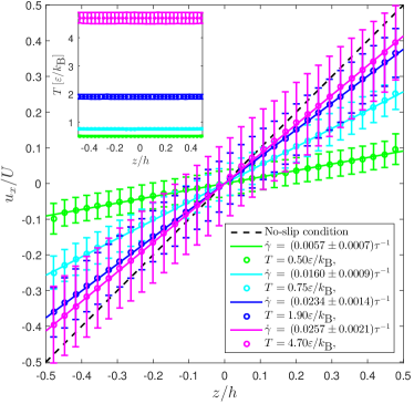
Figure 1: (Color online) Examples of simulation data sets for a steady-state Couette-flow velocity profile, considering $\varepsilon_{fs}=0.2\varepsilon$ and different values of $T$. Linear-regression curves are also shown, as indicated by their respective shear-rate values. The dashed line corresponds to the theoretical profile resulting from the no-slip condition, which is displayed here as a reference. The figure inset shows the corresponding temperature profiles, confirming that the average temperature is uniform across the fluid and equal to the thermostat parameter $T_{b}$.

The shear rate $\dot{\gamma}$ is readily obtained by calculating the slope of a Couette-flow velocity profile. Therefore, the values indicated in the legend of figure 1 were computed by performing linear regressions on the simulation results. Data points corresponding to atomic-scale interfacial nonlinearities were excluded from this fitting procedure, as only the fluid’s bulk region must be considered in the shear-rate assessment. Errors associated with $\dot{\gamma}$ were evaluated by propagating the standard deviations of the velocity profile, in accordance with the usual formulas from basic error analysis.[72, 73]

As evidenced by figure 1, in the case of $\varepsilon_{fs}=0.2\varepsilon$, the shear rate increases with the fluid temperature. Also, note that the velocity profile approaches the situation predicted by the no-slip condition for higher values of $T$. This behavior is opposite to that observed by Wang and Hadjiconstantinou,[60] as only cases corresponding to $T_{c}>0$ in equation (5), implying a monotonically decreasing shear rate, were reported in their work. In our investigation, we also contemplate the possibility of the parameter $T_{c}$ becoming negative, which gives rise to an exponential increase of the slip length as the interface temperature is reduced. Notice that this situation is particularly interesting, as $\lambda$ can reach arbitrarily large values at low temperatures, resulting in the complete deviation from the no-slip condition, possibly even at macroscopic scales. In practice, however, the slip-length value does have an effective upper bound for negative $T_{c}$, which is attained at the threshold of solidification, as the concept of slip length loses its meaning below the fluid’s freezing temperature $T_{F}$.

Figure 2 presents the relationship between the slip length and the fluid temperature for different values of the parameter $\varepsilon_{fs}$, considering only cases in which $T_{c}<0$. This regime, characterized by an upper-unbounded and monotonically-decreasing curve $\lambda(T)$, is designated as the slippery thermal behavior. Each displayed value of $\lambda$ resulted from a single Couette-flow simulation and its error bar was obtained by propagating the associated error found for $\dot{\gamma}$.

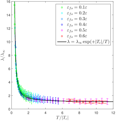
Figure 2: (Color online) Slip length as a function of the fluid temperature for several values of $\varepsilon_{fs}$ resulting in a slippery behavior ($T_{c}<0$).

Note that, in figure 2, $\lambda$ and $T$ are normalized by their corresponding values of $\lambda_{\infty}$ and $|T_{c}|$. In this way, all data sets can be compared to a single reference curve, indicating a universal behavior shared by different interfaces. The parameters $\lambda_{\infty}$ and $T_{c}$ were determined by performing linear regressions with the logarithm of expression (5) as trial function, resulting in the values presented by table 1.

Table 1: Regression results for model function (5).

$\varepsilon_{fs}\;[\varepsilon]$	$\lambda_{\infty}\;[\sigma]$	$T_{c}\;[\varepsilon/k_{B}]$	$R^{2}$
$0.1$	$1.9\pm 0.2$	$-1.98\pm 0.09$	$0.97$
$0.2$	$2.2\pm 0.2$	$-1.51\pm 0.07$	$0.96$
$0.3$	$2.7\pm 0.3$	$-1.03\pm 0.07$	$0.97$
$0.4$	$3.0\pm 0.3$	$-0.63\pm 0.07$	$0.98$
$0.5$	$3.2\pm 0.4$	$-0.31\pm 0.08$	$0.96$
$0.6$	$3.3\pm 0.4$	$-0.07\pm 0.08$	$0.28$
$0.7$	$3.4\pm 0.5$	$+0.24\pm 0.12$	$0.97$
$0.8$	$3.6\pm 0.6$	$+0.53\pm 0.18$	$0.98$
$0.9$	$3.5\pm 0.7$	$+0.76\pm 0.26$	$0.98$
$1.0$	$3.5\pm 0.7$	$+0.94\pm 0.26$	$0.97$
$1.1$	$3.7\pm 1.1$	$+1.33\pm 0.44$	$0.98$
$1.2$	$3.7\pm 1.4$	$+1.48\pm 0.72$	$0.98$

The coefficient of determination $R^{2}$, also shown in table 1, confirms that equation (5) provides a suitable description for the functional relationship between slip length and temperature in the case of slippery interfaces. Observe that the values of $R^{2}$ are close to unity, evidencing the good agreement of the analytical model with the simulation data, except for $\varepsilon_{fs}=0.6$. However, as can be visually verified in figure 2, function (5) does correctly predict the interface’s temperature dependence for all values of the parameter $\varepsilon_{fs}$.

In the critical situation of $\varepsilon_{fs}=0.6$, according to the simulation results, the slip length is practically invariant with respect to temperature. This fact is reflected in the almost null value of the parameter $T_{c}$, which in turn implies that expression (5) is approximately constant. By definition, the coefficient $R^{2}$ provides a quantification of fit quality by comparing the proposed model function to the average value of the dependent variable. Therefore, in the case where the trial curve corresponds to a constant, no conclusions can be drawn from $R^{2}$, thus explaining the coefficient’s small value for $\varepsilon_{fs}=0.6$.

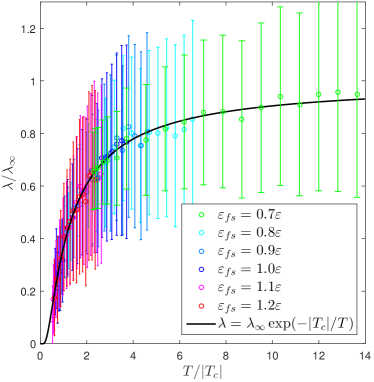
Figure 3: (Color online) Slip-length values as a function of the fluid temperature for several values of $\varepsilon_{fs}$ resulting in a sticky behavior ($T_{c}>0$).

Simulation data portraying the slip length as a function of the fluid temperature is again shown in figure 3, now considering values of the parameter $\varepsilon_{fs}$ corresponding to $T_{c}>0$. Similarly to the preceding case, the variables $\lambda$ and $T$ were normalized by their respective values of $\lambda_{\infty}$ and $|T_{c}|$, allowing comparison with a single reference curve. Obtained values of $\lambda_{\infty}$, $T_{c}$, and $R^{2}$, resulting from linear regressions using the logarithm of function (5), are also found in table 1.

As can be visually inferred from figure 3 and confirmed by the close-to-unity values of $R^{2}$, expression (5) appropriately describes the temperature dependence of interfacial slip also for positive $T_{c}$. In this situation, the model function $\lambda(T)$ is monotonically increasing and bounded between zero and $\lambda_{\infty}$. As a consequence, if two distinct hypothetical interfaces are considered, with identical values of $\lambda_{\infty}$ and $|T_{c}|$, but opposite signs of the characteristic temperature, the slip length of the interface with positive $T_{c}$ will be strictly lower for any finite fluid temperature. The difference between the two cases is even more evident for low temperatures ($T\ll|T_{c}|$), as $\lambda$ approaches zero for $T_{c}>0$, while it goes to infinity for $T_{c}<0$. For these reasons, the regime of positive $T_{c}$ is designated as the sticky thermal behavior.

According to table 1, in both slippery and sticky cases, the value of $\lambda_{\infty}$ slowly increases as the parameter $\varepsilon_{fs}$ is raised. The increase rate is different for each of the thermal behaviors, being clearly faster in the slippery regime. Therefore, albeit counterintuitive, simulation data does indicate that stronger interface interactions result in larger slip lengths at high fluid temperatures ($T\gg|T_{c}|$).

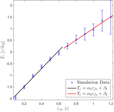
Figure 4: (Color online) Dependence of $T_{c}$ on the fluid-solid interaction parameter $\varepsilon_{fs}$.

As expected from equation (6), the parameter $T_{c}$ linearly increases with the interaction strength $\varepsilon_{fs}$. However, as shown in figure 4, different values of the adjustable coefficients $\alpha$ and $\beta$ are found for each thermal behavior, once again indicating profound changes in the interfacial properties as the slippery-sticky transition takes place. For $T_{c}<0$, a linear-regression analysis provides $\alpha_{1}=(3.9\pm 0.2)k_{B}^{-1}$ and $\beta_{1}=(-2.26\pm 0.07)\varepsilon/k_{B}$ with coefficient of determination $R^{2}=0.984$. Similarly, for $T_{c}>0$, the values $\alpha_{2}=(2.5\pm 0.7)k_{B}^{-1}$ and $\beta_{2}=(-1.50\pm 0.55)\varepsilon/k_{B}$ are obtained, with $R^{2}=0.991$. Notice that, in both cases, high agreement between the model function and the numerical simulations is evinced by the coefficient $R^{2}$.

By employing the fitted curves of figure 4, the value of the parameter $\varepsilon_{fs}$ at which the slippery-stick transition occurs can be readily determined. This critical fluid-solid interaction strength, denoted by $\tilde{\varepsilon}_{fs}$, directly follows from equation (6) by setting $T_{c}=0$, that is, $\tilde{\varepsilon}_{fs}=-\beta/\alpha$. This relation yields $\tilde{\varepsilon}_{fs,1}=(0.59\pm 0.03)\varepsilon$, for negative $T_{c}$, and $\tilde{\varepsilon}_{fs,2}=(0.60\pm 0.27)\varepsilon$, for positive $T_{c}$. Note that the values of $\tilde{\varepsilon}_{fs,1}$ and $\tilde{\varepsilon}_{fs,2}$ agree within errors, as required for consistency and continuity, since both curves for $T_{c}(\varepsilon_{fs})$ are expected to meet at the critical parameter. In addition, the two estimates for $\tilde{\varepsilon}_{fs}$ suggest that its true value is close to $0.6\varepsilon$, as could be inferred from figure 2, due to the approximately constant behavior of $\lambda(T)$ at this interaction strength.

IV Discussion

As shown in the previous section, both slippery and sticky thermal behaviors were adequately described by a previously-proposed model function,[60] which was linearly fitted to our simulation data, thus determining the adjustable parameters $\lambda_{\infty}$ and $T_{c}$. It is particularly interesting to note that this analytical model also correctly portrays the slippery regime, although its original authors seem to have devised it with only the sticky case in mind. As mentioned earlier, in the derivation outlined by Wang and Hadjiconstantinou, the fluid-slip phenomenon is understood as a thermally-activated hopping process, where the thermal energy enables fluid particles to overcome potential barriers. Therefore, in this context, the existence of interfaces for which slip length decreases with temperature appears to be counterintuitive.

Within the slippery regime, the characteristic temperature $T_{c}$ is negative, meaning that the model’s total energy barrier $V_{fs}+V_{ff}=k_{B}T_{c}$ is actually a potential well, promoting the movement of fluid particles along the solid surface. This slip-facilitating mechanism is gradually suppressed by increasing the thermal fluctuations, as they may cause the entrapment of fluid particles in the potential wells.

In general, interfacial fluid particles are subjected to a competition between cohesive and adhesive forces. Seeking to maintain cohesion, forces originating from the fluid are responsible for the term $V_{ff}=k_{B}\beta$, which is always negative, as follows from the values of $\beta_{1}$ and $\beta_{2}$ presented in section III. On the other hand, the adhesive forces from the solid surface result in the term $V_{fs}=k_{B}\alpha\varepsilon_{fs}$, which is strictly positive, as evinced by the obtained values of $\alpha_{1}$ and $\alpha_{2}$. Therefore, the slippery behavior occurs when the fluid cohesion at the interface is stronger than the adhesion to the solid surface ($|V_{ff}|>|V_{fs}|$). In the opposite situation, the sticky behavior arises.

The slippery-sticky transition takes place at the critical interaction-strength value $\tilde{\varepsilon}_{fs}$, for which the characteristic temperature vanishes or, equivalently, the energy contributions $V_{fs}$ and $V_{ff}$ cancel each other out. In this particular situation, fluid particles experience a smooth average energy landscape at the interface, so that thermal mechanisms of hopping and entrapment are absent, resulting in the slip length’s temperature invariance. Consequently, at the transition, the slip-length value is solely determined by other physical properties, such as viscosity and surface density.

In section III, by examining the dependence of $T_{c}$ on the fluid-solid interaction strength, the value of $\tilde{\varepsilon}_{fs}$ was determined to be approximately $0.6\varepsilon$. Interestingly, in addition to its sign change, the curve $T_{c}(\varepsilon_{fs})$ also exhibits a slope discontinuity at the transition. Therefore, the characteristic temperature signals the slippery-sticky transition in two different ways, establishing itself as a reliable identifier parameter for the slip length’s thermal behavior.

Finally, we would like to point out the relevance of $|T_{c}|$ to the interfacial thermal behavior, particularly when compared to the fluid’s freezing temperature $T_{F}$, since the latter represents the lower bound of the temperature range in which the present analysis is valid. As previously discussed, for small absolute values of the characteristic temperature ($|T_{c}|\ll T_{F}$), the slip length is almost independent of $T$. In general, for $|T_{c}|$ below the fluid’s freezing temperature $T_{F}$, $\lambda(T)$ is a slowly varying function within the accessible temperature range. On the other hand, for $|T_{c}|>T_{F}$, $\lambda(T)$ can present actual exponential behavior for sufficiently low temperatures ($T\ll|T_{c}|$), quickly bringing the slip-length value to zero or taking it to infinite, depending on the sign of $T_{c}$, as can be observed in figures 2 and 3. Therefore, if a technological application demands an exceptionally slippery or sticky interface, the interacting materials should be chosen in such a way as to provide the highest possible value of $|T_{c}|$, so that the system’s working temperature is comparatively low and, consequently, an appropriate slip length is attainable.

V Conclusion

By performing molecular-dynamics simulations of a Couette flow, composed of a Lennard-Jones fluid at constant density and simple-cubic rigid walls, the temperature effects on fluid slip were thoroughly examined. As shown in section III, the slip length can present two completely different thermal behaviors depending on the interaction strength between the fluid and the solid surfaces. In the slippery case, corresponding to weak interface interactions ($\varepsilon_{fs}<\tilde{\varepsilon}_{fs}$), the slip-length value is upper-unbounded and decreases with temperature. On the other hand, for strong fluid-solid interactions ($\varepsilon_{fs}>\tilde{\varepsilon}_{fs}$), the interface displays the sticky behavior, characterized by slip-length values increasing with temperature, but in a restricted interval.

From a technological point of view, interfaces capable of operating in the slippery regime are very promising. Assuming that the slippery thermal behavior is not hindered by other effects, the arbitrarily large slip lengths obtainable at low temperatures ($T\ll|T_{c}|$) could be readily exploited in applications requiring low frictional stress. From a design perspective, the determination of characteristic temperatures, either empirically or numerically, provides a searching path for the development or selection of materials for such friction-reduction purposes. As previously discussed, large-magnitude negative values of $T_{c}$ will make the slippery behavior more appreciable at higher temperatures, ideally far above the fluid’s solidification temperature $T_{F}$.

The present work’s findings, in conjunction with the analytical model proposed in reference [60], can assist in devising methods for the efficient simulation of continuum fluidic systems in which interfacial boundary conditions are required to be sensitive to nonuniform temperature distributions. By performing a small set of molecular-dynamics simulations, the parameters $\lambda_{\infty}$ and $T_{c}$ can be promptly determined for a fluid-solid interface of interest. Upon substituting these values into the slip-length model function (5) and then inserting the resulting expression into equation (1), the velocity-field boundary conditions at interfaces displaying spatial or temporal temperature variations can be readily specified, giving rise to a hierarchical multiscale approach to fluid dynamics.[15]

Clearly, the physical interpretation of our results, as laid out in section III, strongly relies on the model proposed in reference [60]. Despite this, the present work should not be viewed as an attempt to access the microscopic validity of Wang and Hadjiconstantinou’s model, that is, whether the thermal hopping and entrapment mechanisms, besides providing a useful conceptualization of the slip phenomenon, actually take place in reality. Rather, our core result is the observation that, concerning the slip phenomenon in a simple interface system, two distinct thermal behaviors can occur depending on the fluid-solid interaction parameter, an observation purely based on numerical simulations. The reported data, nonetheless, provide new evidence in favor of the model, namely, the particularly compelling fact that it is capable of correctly describing both observed behaviors while also endowing the results with an insightful explanation that fits well within the reaction-rate picture, as discussed in section IV. The investigation of the analytical model’s microscopic realism is a very interesting topic, which we will hopefully address in future work.

Finally, note that the results of section III are reasonably general. That is, by adopting a system of units based on the fluid’s fundamental properties and defining the fluid-solid interaction parameters relative to it, a representative discussion is provided for any interface whose intermolecular forces can be effectively described by Lennard-Jones potentials. However, for more complex interparticle interactions, other effects beyond those considered in the present study could influence the slip length’s temperature dependence, so that it would be erroneous to conclude that the slippery and sticky behaviors, as described by function (5) and portrayed by figures 2 and 3, will be observed in more sophisticated interface models. Nevertheless, even in more complicated scenarios, the mechanisms investigated in this work still participate in the system dynamics, and they will have a role in determining the interfacial fluid slip. This is because the repulsive and van der Waals interactions following from the Lennard-Jones potential are essential ingredients of more elaborated force fields, which will typically also include long-range Coulomb forces as well as other terms that account for the internal degrees of freedom of each molecule. Whether the Lennard-Jones contribution has a generally dominant or negligible role in determining the slip length’s thermal behavior in such complex systems remains an open question that we intend to tackle in future studies.

Data Availability

The data that support the findings of this study are available from the corresponding author upon reasonable request.

Appendix A Simulation Details

This appendix presents further details on the adopted methodology and employed algorithms. In particular, the parameter values which remain fixed across all numerical simulations in section III are provided here.

Firstly, we point out that an in-house code was used for performing the molecular-dynamics simulations. A representative subset of the obtained data was also compared to its equivalent counterpart generated with the aid of the LAMMPS package,[75] yielding similar results within error bars.

As mentioned in subsection II.2, the fluid particles interact with one another through the truncated and smoothed Lennard-Jones potential, with its parameters $\sigma$ and $\varepsilon$ serving as a reference for the system of units. In addition, the cutoff radius of fluid-fluid interactions receives the customary value $r_{c}^{ff}=2.5\sigma$. In all considered simulations, the fluid is composed of $12000$ particles, which occupy a channel of width $h=32.18\sigma$, specifically chosen to avoid the occurrence of confinement effects, as determined by early investigations. The $x$ and $y$ directions of the simulation box, in which periodic boundary conditions are assumed, have the same length $L=21.45\sigma$. Considering the channel’s available volume $\mathcal{V}_{f}=hL^{2}$, notice that the fluid has average density $\rho_{f}=0.81\sigma^{-3}$. Additionally, in order to properly control the fluid temperature, equation (3) is employed with damping coefficient $\Gamma=1.0\tau^{-1}$.

The planar Couette flow is generated by two flat plates moving in parallel with relative speed $U=1.0\sigma/\tau$. These rigid walls have simple-cubic crystal structure, with their $(001)$ planes facing the fluid and their atoms aligned parallel to the specified Cartesian directions. Each solid surface is composed of $6936$ particles, arranged in a layer of thickness $h_{s}=3.78\sigma$ and average density $\rho_{s}=4.0\sigma^{-3}$. The atomic structure, density, and velocity of the plates were chosen in order to accentuate the fluid-slip phenomenon, in agreement with preliminary simulations. These earlier investigations have shown that increasing the shear rate, by raising the plate velocities, implies larger slip-length values, as intuitively expected and demonstrated by other authors.[23, 24] Interfacial slip was also found to occur more intensely for solids with higher particle densities, in accordance with the idea that a more compact crystal structure displays a smoother surface thus impairing tangential momentum transfer. Additionally, the simple-cubic structure was found to yield the largest slip lengths among the cubic lattices.

The solid-surface particles are restricted to uniform linear motion, with velocity $+U\hat{x}/2$ in the upper plate and $-U\hat{x}/2$ in the lower one. Accordingly, these particles are not subject to forces from the fluid or the solid surface itself. Although there is no reaction, wall atoms act on the fluid through the truncated and smoothed Lennard-Jones potential with fixed parameters $\sigma_{fs}=0.75\sigma$ and $r_{c}^{fs}=2.5\sigma_{fs}$. Note that the range of the fluid-solid interaction is appropriately smaller than the plate thickness $h_{s}$, so that the fluid particles are unable to ‘perceive’ the solid surfaces as finite objects.

The numerical integration of the dynamical system, composed of coupled Langevin equations, is performed by a leapfrog integrator, considering fixed time steps of length $\Delta t=5\times 10^{-3}\tau$. The Couette-flow simulation is divided into two stages. In a first phase, lasting $\mathcal{T}=5\times 10^{5}\Delta t=2.5\times 10^{3}\tau$, the fluid, initially at rest, is sheared by the solid surfaces until the steady state is reached. As initial atomic positions, fluid particles are positioned in a regular lattice with random-direction velocities, whose magnitudes are chosen so that each atom’s kinetic energy conforms to the target temperature $T_{b}$. In a second phase, also of duration $\mathcal{T}$, the values of all pertinent physical quantities are collected at each time step.

During the data-gathering stage, the simulation box is divided along the $z$ direction into $40$ slabs of identical thickness. In this way, instantaneous values of the fluid’s density, velocity, and temperature profiles are evaluated, considering respectively the number, the mean velocity, and the mean thermal-kinetic energy of the particles in each partition. Time averages and their respective standard deviations are then calculated by taking into account all time steps in the period $\mathcal{T}$. Note that, according to this procedure, the standard deviations are proportional to the fluctuation amplitudes of the physical quantities during their time series.

In order to properly investigate the slip length’s temperature dependence, molecular-dynamics simulations were performed with temperature values between $0.1\varepsilon/k_{B}$ and $3.5\varepsilon/k_{B}$ for each choice of the parameter $\varepsilon_{fs}$. Since part of this range lies below the Lennard-Jones equilibrium freezing temperature, approximately $0.69\varepsilon/k_{B}$, some of the low-temperature runs naturally resulted in systems displaying no fluidic behavior and, consequently, were discarded from the fluid-slip analysis. In other words, only those simulations presenting a steady-state characterized by a linear and symmetrical bulk velocity profile, as well as uniform bulk temperature and density profiles, after the period $\mathcal{T}$ of system preparation, were effectively considered in the slip-length evaluation.

Linear regressions, employed in the determination of shear-rate values and the adjustable parameters in expressions (5) and (6), were performed with the method of least squares, considering the inverse squared errors of the dependent variables as summation weights.[73]

References

- Lyklema [1995] J. Lyklema, Fundamentals of interface and colloid science. Volume 2: Solid-liquid interfaces (Academic Press, 1995).
- Wandelt and Thurgate [2002] K. Wandelt and S. Thurgate, Solid-Liquid Interfaces: Macroscopic Phenomena-Microscopic Understanding, Vol. 85 (Springer Science & Business Media, 2002).
- Wang [2008] X. S. Wang, Fundamentals of fluid-solid interactions: analytical and computational approaches (Elsevier, 2008).
- Xing [2019] J. T. Xing, Fluid-Solid Interaction Dynamics: Theory, Variational Principles, Numerical Methods, and Applications (Academic Press, 2019).
- Navier [1823] C. L. M. H. Navier, Mémoires de l’Académie Royale des Sciences de l’Institut de France 6, 389 (1823).
- Day [1990] M. A. Day, Erkenntnis 33, 285 (1990).
- Lauga et al. [2007] E. Lauga, M. Brenner, and H. Stone, in Springer Handbook of Experimental Fluid Mechanics (Springer, 2007) pp. 1219–1240.
- Landau and Lifshitz [1987] L. D. Landau and E. M. Lifshitz, Fluid Mechanics (Pergamon Press, 1987).
- Batchelor [2000] G. K. Batchelor, An Introduction to Fluid Dynamics (Cambridge university press, 2000).
- Sokhan et al. [2002] V. P. Sokhan, D. Nicholson, and N. Quirke, The Journal of Chemical Physics 117, 8531 (2002).
- Thomas and McGaughey [2008] J. A. Thomas and A. J. H. McGaughey, Nano Letters 8, 2788 (2008).
- Liu and Li [2011] C. Liu and Z. Li, AIP Advances 1, 032108 (2011).
- Allen and Tildesley [1987] M. P. Allen and D. J. Tildesley, Computer Simulation of Liquids (Oxford university press, 1987).
- Rapaport [2004] D. C. Rapaport, The Art of Molecular Dynamics Simulation (Cambridge University Press, 2004).
- Viscondi et al. [2019] T. F. Viscondi, A. Grigolo, J. A. P. Aranha, J. R. C. Piqueira, I. L. Caldas, and J. R. Meneghini, Polytechnica 2, 77 (2019).
- Lichter et al. [2004] S. Lichter, A. Roxin, and S. Mandre, Physical Review Letters 93, 086001 (2004).
- Lichter et al. [2007] S. Lichter, A. Martini, R. Q. Snurr, and Q. Wang, Physical Review Letters 98, 226001 (2007).
- Martini et al. [2008a] A. Martini, A. Roxin, R. Q. Snurr, Q. Wang, and S. Lichter, Journal of Fluid Mechanics 600, 257 (2008a).
- Yong and Zhang [2010] X. Yong and L. T. Zhang, Physical Review E 82, 056313 (2010).
- Sochi [2011] T. Sochi, Polymer Reviews 51, 309 (2011).
- Wang and Zhao [2011] F.-C. Wang and Y.-P. Zhao, Soft Matter 7, 8628 (2011).
- Yong and Zhang [2013] X. Yong and L. T. Zhang, Microfluidics and Nanofluidics 14, 299 (2013).
- Thompson and Troian [1997] P. A. Thompson and S. M. Troian, Nature 389, 360 (1997).
- Priezjev [2007a] N. V. Priezjev, Physical Review E 75, 051605 (2007a).
- Xu and Li [2007] J. Xu and Y. Li, International Journal of Heat and Mass Transfer 50, 2571 (2007).
- Ramos-Alvarado et al. [2016a] B. Ramos-Alvarado, S. Kumar, and G. P. Peterson, Physical Review E 93, 023101 (2016a).
- Koplik et al. [1989] J. Koplik, J. R. Banavar, and J. F. Willemsen, Physics of Fluids A: Fluid Dynamics 1, 781 (1989).
- Cieplak et al. [2001] M. Cieplak, J. Koplik, and J. R. Banavar, Physical Review Letters 86, 803 (2001).
- Martini et al. [2008b] A. Martini, H.-Y. Hsu, N. A. Patankar, and S. Lichter, Physical Review Letters 100, 206001 (2008b).
- Asproulis and Drikakis [2010] N. Asproulis and D. Drikakis, Physical Review E 81, 061503 (2010).
- Asproulis and Drikakis [2011] N. Asproulis and D. Drikakis, Physical Review E 84, 031504 (2011).
- Pahlavan and Freund [2011] A. A. Pahlavan and J. B. Freund, Physical Review E 83, 021602 (2011).
- Guo et al. [2005] Z. Guo, T. S. Zhao, and Y. Shi, Physical Review E 72, 036301 (2005).
- Servantie and Müller [2008] J. Servantie and M. Müller, Physical Review Letters 101, 026101 (2008).
- Bao et al. [2017] L. Bao, N. V. Priezjev, H. Hu, and K. Luo, Physical Review E 96, 033110 (2017).
- Barrat and Bocquet [1999a] J.-L. Barrat and L. Bocquet, Physical Review Letters 82, 4671 (1999a).
- Barrat and Bocquet [1999b] J.-L. Barrat and L. Bocquet, Faraday Discussions 112, 119 (1999b).
- Nagayama and Cheng [2004] G. Nagayama and P. Cheng, International Journal of Heat and Mass Transfer 47, 501 (2004).
- Voronov et al. [2006] R. S. Voronov, D. V. Papavassiliou, and L. L. Lee, The Journal of Chemical Physics 124, 204701 (2006).
- Voronov et al. [2007] R. S. Voronov, D. V. Papavassiliou, and L. L. Lee, Chemical Physics Letters 441, 273 (2007).
- Voronov et al. [2008] R. S. Voronov, D. V. Papavassiliou, and L. L. Lee, Industrial & Engineering Chemistry Research 47, 2455 (2008).
- Huang et al. [2008] D. M. Huang, C. Sendner, D. Horinek, R. R. Netz, and L. Bocquet, Physical Review Letters 101, 226101 (2008).
- Sendner et al. [2009] C. Sendner, D. Horinek, L. Bocquet, and R. R. Netz, Langmuir 25, 10768 (2009).
- Ho et al. [2011] T. A. Ho, D. V. Papavassiliou, L. L. Lee, and A. Striolo, Proceedings of the National Academy of Sciences (2011).
- Huang and Szlufarska [2012] K. Huang and I. Szlufarska, Langmuir 28, 17302 (2012).
- Ramos-Alvarado et al. [2016b] B. Ramos-Alvarado, S. Kumar, and G. P. Peterson, Applied Physics Letters 108, 074105 (2016b).
- Yen and Soong [2016] T.-H. Yen and C.-Y. Soong, Molecular Physics 114, 797 (2016).
- Liu and Li [2009] C. Liu and Z. Li, Physical Review E 80, 036302 (2009).
- Liu and Li [2010] C. Liu and Z. Li, The Journal of Chemical Physics 132, 024507 (2010).
- Semiromi and Azimian [2010] D. T. Semiromi and A. R. Azimian, Heat and Mass Transfer 46, 791 (2010).
- Sofos et al. [2013] F. Sofos, T. E. Karakasidis, and A. Liakopoulos, Journal of Computational and Theoretical Nanoscience 10, 648 (2013).
- Jabbarzadeh et al. [2000] A. Jabbarzadeh, J. D. Atkinson, and R. I. Tanner, Physical Review E 61, 690 (2000).
- Cottin-Bizonne et al. [2003] C. Cottin-Bizonne, J.-L. Barrat, L. Bocquet, and E. Charlaix, Nature Materials 2, 237 (2003).
- Cottin-Bizonne et al. [2004] C. Cottin-Bizonne, C. Barentin, É. Charlaix, L. Bocquet, and J.-L. Barrat, The European Physical Journal E 15, 427 (2004).
- Galea and Attard [2004] T.-M. Galea and P. Attard, Langmuir 20, 3477 (2004).
- Priezjev et al. [2005] N. V. Priezjev, A. A. Darhuber, and S. M. Troian, Physical Review E 71, 041608 (2005).
- Priezjev and Troian [2006] N. V. Priezjev and S. M. Troian, Journal of Fluid Mechanics 554, 25 (2006).
- Priezjev [2007b] N. V. Priezjev, The Journal of Chemical Physics 127, 144708 (2007b).
- Niavarani and Priezjev [2010] A. Niavarani and N. V. Priezjev, Physical Review E 81, 011606 (2010).
- Wang and Hadjiconstantinou [2019] G. J. Wang and N. G. Hadjiconstantinou, Physical Review Fluids 4, 064201 (2019).
- Note [1] The layering effect is the well-known phenomenon of induced structuring of fluid molecules at the vicinity of a solid wall, causing oscillations of a characteristic wavelength in the fluid’s density profile along the surface’s normal direction. In our interface model, which is based on short-range Lennard-Jones interactions, these oscillations are observed only within a few molecular diameters away from the solid plates, so that the density is always uniform in the bulk region, where all measurements are made. Still, since different numbers of particles accumulate in the structured layers for different values of , and since the total number of fluid particles is the same for all simulations, the bulk density varies slightly across runs. As mentioned in the text, this variation in bulk density is negligible for our purposes.
- Hansen and Verlet [1969] J.-P. Hansen and L. Verlet, Physical Review 184, 151 (1969).
- Khrapak et al. [2010] S. A. Khrapak, M. Chaudhuri, and G. E. Morfill, Physical Review B 82, 052101 (2010).
- Schultz and Kofke [2018] A. J. Schultz and D. A. Kofke, The Journal of Chemical Physics 149, 204508 (2018).
- Stephan et al. [2019] S. Stephan, M. Thol, J. Vrabec, and H. Hasse, Journal of Chemical Information and Modeling 59, 4248 (2019).
- Eyring [1936] H. Eyring, The Journal of Chemical Physics 4, 283 (1936).
- Hirschfelder et al. [1964] J. O. Hirschfelder, C. F. Curtiss, R. B. Bird, and M. G. Mayer, Molecular theory of gases and liquids, Vol. 165 (Wiley New York, 1964).
- Hänggi et al. [1990] P. Hänggi, P. Talkner, and M. Borkovec, Reviews of Modern Physics 62, 251 (1990).
- Blake and Haynes [1969] T. D. Blake and J. M. Haynes, Journal of Colloid and Interface Science 30, 421 (1969).
- Brochard-Wyart and Gennes [1992] F. Brochard-Wyart and P. G. D. Gennes, Simple Views On Condensed Matter 4, 349 (1992).
- Wang and Hadjiconstantinou [2017] G. J. Wang and N. G. Hadjiconstantinou, Physical Review Fluids 2, 094201 (2017).
- Taylor [1997] J. R. Taylor, An Introduction to Error Analysis (University Science Books, 1997).
- Bevington and Robinson [2003] P. R. Bevington and D. K. Robinson, Data Reduction and Error Analysis (McGraw Hill, 2003).
- Note [2] Other potentially relevant interface properties, such as the fluid-solid radial distribution function and fluid’s density profile close to the solid surface, were also examined as functions of temperature for several values of the fluid-solid interaction strength. No remarkably discriminating behavior was observed in these quantities when comparing slippery and sticky interfaces. In general, these observables change continuously with , showing no evident sign of the transition at . For this reason, we chose not to show these negative results here.
- Plimpton [1995] S. Plimpton, Journal of computational physics 117, 1 (1995).