Removing Diffraction Image Artifacts in Under-Display Camera via
Dynamic Skip Connection Network

Abstract

Recent development of Under-Display Camera (UDC) systems provides a true bezel-less and notch-free viewing experience on smartphones (and TV, laptops, tablets), while allowing images to be captured from the selfie camera embedded underneath. In a typical UDC system, the microstructure of the semi-transparent organic light-emitting diode (OLED) pixel array attenuates and diffracts the incident light on the camera, resulting in significant image quality degradation. Oftentimes, noise, flare, haze, and blur can be observed in UDC images. In this work, we aim to analyze and tackle the aforementioned degradation problems. We define a physics-based image formation model to better understand the degradation. In addition, we utilize one of the world’s first commodity UDC smartphone prototypes to measure the real-world Point Spread Function (PSF) of the UDC system, and provide a model-based data synthesis pipeline to generate realistically degraded images. We specially design a new domain knowledge-enabled Dynamic Skip Connection Network (DISCNet) to restore the UDC images. We demonstrate the effectiveness of our method through extensive experiments on both synthetic and real UDC data. Our physics-based image formation model and proposed DISCNet can provide foundations for further exploration in UDC image restoration, and even for general diffraction artifact removal in a broader sense.

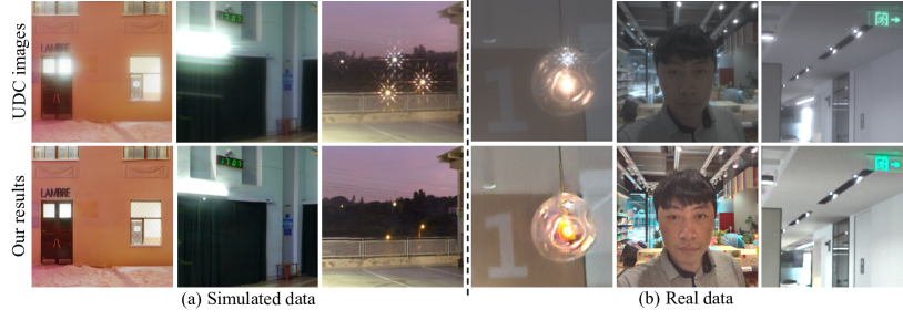
Figure 1: Removing Diffraction Artifacts from Under-Display Camera (UDC) images. The major degradations caused by light diffraction, e.g., flare, blur, and haze, could significantly affect the visual quality of UDC images. Our method effectively restores fine details and suppresses the diffraction effects of UDC images.

1 Introduction

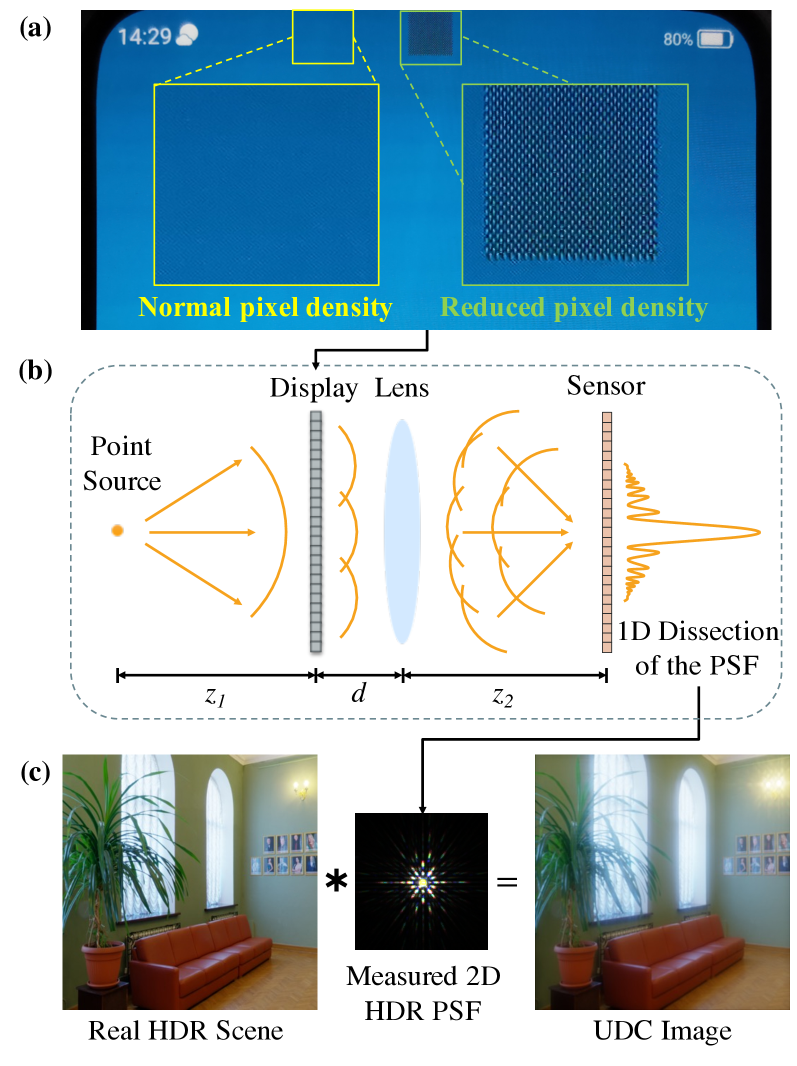
Figure 2: (a) A close-up shot of the UDC OLED on the ZTE Axon 20 phone. The UDC OLED panel has reduced pixel density in the area above the camera, allowing for more transparency. (b) The schematic of the UDC system. The light emitted from a point light source is modulated by the OLED and camera lens, before being captured by the sensor. (c) A simulated example of our image formation model with a real-captured PSF. The 2D PSF is brightened in the figure to visualize the structured sidelobe patterns.

The consumer demand for smartphones with bezel-free, notch-less display has sparked a surge of interest from the phone manufacturers in a newly-defined imaging system, Under-Display Camera (UDC). Besides smartphones, UDC also demonstrates its practical applicability in other scenarios, i.e., for videoconferencing with UDC TV, laptops, or tablets, enabling more natural gaze focus as they place cameras at the center of the displays [16]. As Figure 2 shows, a typical UDC system has the camera module placed underneath and closely attached to the semi-transparent Organic Light-Emitting Diode (OLED) display. Although the display looks partially transparent, the regions where the light can pass through, i.e.the gaps between the display pixels, are usually in the micrometer scale, which substantially diffracts the incoming light [23], affecting the light propagation from the scene to the sensor. The UDC systems introduce a new class of complex image degradation problems, combining strong flare, haze, blur, and noise (see top row in Figure Removing Diffraction Image Artifacts in Under-Display Camera via Dynamic Skip Connection Network). In the first attempt [47] to address the UDC image restoration problem, the authors proposed a Monitor-Camera Imaging System (MCIS) to capture paired data and used the image formation to synthesize the Point Spread Function (PSF) of two types of OLED display. However, there are several drawbacks of this pioneer work, including 1) inaccurate PSF due to a mismatch between the actual and the synthetic PSF, 2) lacking proper high dynamic range (HDR) in the MCIS-captured data, missing realistic UDC degradation, 3) prototype UDC differs significantly from actual production UDC, 4) missing real-world evaluation on non-MCIS data, and 5) proposed network does not fully utilize domain knowledge. We examine the drawbacks in further details in Section 2.

In this work, we aim to address the aforementioned issues. We first present a realistic image formation model and measurement protocol considering proper dynamic range for the scenes and camera sensor, and restore the real-world degradation in the actual UDC images. To this end, we experiment with one of the world’s first production UDC device, ZTE Axon 20, which incorporates a UDC system into its selfie camera. Note that we aim to analyze and investigate the artifacts caused by diffraction effects, rather than propose a product-ready solution for ZTE phone camera. Our method is versatile and applicable to other UDC device, or more generally, other diffraction-limited imaging systems, e.g., microscopy imaging, pinhole camera. We devise an imaging system to directly measure the PSF of the UDC device (see Section 3.2) with a point source. As shown in Figure 2, due to the diffraction of the display, the resulting PSF has some special characteristics: it has large spatial support, strong response at the center, and long-tail low-energy sidelobes. With the measured PSF, we reformulate the image formation model to account for realistic flare, haze, and blur, which were missing [46, 47] due to the limited dynamic range of scenes. Then, we develop a data simulation pipeline based on the image formation model by using HDR images to approximate real scenes. Additionally, we capture real images using the UDC phone’s selfie camera to validate our simulated data and evaluate the performance of our restoration network. As shown in Figure Removing Diffraction Image Artifacts in Under-Display Camera via Dynamic Skip Connection Network, our simulated and real data reveal similar degradation, especially in those high-intensity regions. Specifically, flare can be observed nearby strong light sources, where highlights are spread into neighboring low-intensity areas in structured diffraction patterns.

To restore the UDC images, we propose a DynamIc Skip Connection Network (DISCNet) that incorporates the domain knowledge of the image formation model into the network designs. In particular, sensor saturation breaks the shift-invariance of the single-PSF-based convolution, leading to spatially-variant degradation. This motivates us to design a dynamic filter network to dynamically predict filters for each pixel. In addition, due to large support of PSF, we propose a multi-scale architecture and perform dynamic convolution in the feature domain to obtain a larger receptive field. Also, a condition encoder is introduced to utilize the information of PSF.

In summary, our contributions are as follows:

• We reformulate the image formation model for UDC systems by considering dynamic range and saturation, which takes into account the diffraction flare commonly seen in UDC images.

• We utilize the first UDC smartphone prototypes to measure the real-world PSF. The PSF is used as part of a model-based data synthesis pipeline to generate realistic degraded images.

• We devise a DynamIc Skip Connection Network (DISCNet) that incorporates the domain knowledge of the UDC image formation model. Experimental results show that it is effective for removing diffraction image artifacts in UDC systems.

2 Related Work

UDC Imaging. Several previous work [24, 32] characterized and analyzed the diffraction effects of UDC systems. Kwon et al.[13] modeled the edge spread function of transparent OLED. Qin et al.[23] discussed pixel structure design that can potentially reduce the diffraction. While all these works provide good insights into UDC imaging systems, none of them tackles the image restoration problem. Additionally, several works [8, 30, 29] proposed camera-behind-display design for enhanced 3D interaction with flat panel display. Though low-resolution images are the by-products of those prototype interaction systems, given the extremely poor image quality, they are unsuitable for daily photography, which is the focus of this work.

UDC Restoration. To our best knowledge, [47] and the subsequent ECCV challenge [46] are the only works that directly address the problem of UDC image restoration. In [47], the authors devised an MCIS to capture paired images, and solve the UDC image restoration problem as a blind deconvolution problem using a variant of UNet [26]. While the work pioneers the UDC image restoration problem, it suffers from several drawbacks.

First, while MCISs are commonly used in the computational imaging community [22, 1] to capture the system PSF or acquire paired image data, most commodity monitor lacks the high dynamic range which is a must to model realistic diffraction artifacts in UDC systems. As a result, the PSFs they used have incomplete side lobes, and the images have less severe artifacts, e.g., blur, haze, and flare. In our work, we consider HDR in data generation and PSF measurement to allow us to tackle real-world scenes properly. Secondly, the authors use regular OLED manually covering a camera in their setup, instead of an actual rigid UDC assembly, and perform experiments and evaluations on quasi-realistic data. As a result, any slight movements, rotation, or tilt of the display with respect to the sensor plane will cause variational PSFs, preventing their network from being applied to handle variational degradations without the knowledge of the PSF kernel. To minimize the domain gap, we use one of the world’s first production UDC device for data collection, experiments, and evaluations. Lastly, though the authors captured and used the PSF in data synthesis, they formulated the UDC image restoration as a blind deconvolution problem through a simple UNet, without explicitly utilizing the PSFs as useful domain knowledge. In contrast, we leverage the PSF as important supporting information in our proposed DISCNet.

Non-blind Image Restoration. In the context of non-blind image restoration, a large body of works has exerted great effort to tackle this ill-posed problem. Prior to the deep-learning era, early deconvolution approaches [25, 20, 14, 4, 36] imposed prior knowledge to constrain the solution space since the noise model is unknown. Then, several works [27, 37, 41] focused on establishing the connection between optimization-based deconvolution and a neural network for non-blind image restoration. Also, Shocher et al.[28] employed a small image-specific network to deal with various degradations of a single image. Zhang et al.[42] proposed SRMD to handle multiple degradations with one network. Gu et al.[5] proposed SFTMD and Iterative Kernel Correction (IKC) to iteratively correct the kernel code of degradations. Additionally, [3, 40, 44] used Generative Adversarial Networks (GANs) to tackle different degradations. Similar to SRMD [42], we take the PSF kernel as an additional condition but use it in a different way, i.e., feed it into a condition encoder to facilitate dynamic filter generation.

Dynamic Filter Network. Recent years have witnessed great success in dynamic filter networks employed in a wide range of vision applications to handle spatially-variant issues. Jia et al.[9] firstly exploited dynamic network to generate an individual kernel for each pixel conditioned on the input image. Since then, this module has proven to provide significant benefits for applications, such as video interpolation [18, 19], denoising [2, 17, 38], super-resolution [10, 39, 34], and video deblurring [45]. In addition, Wang et al.[33] proposed a kernel prediction module serving as a universal upsampling operator. Most previous approaches, however, can not be directly applied to UDC image restoration, because they either apply predicted filters in the image domain or mainly focus on a special operation. In this work, we construct multi-scale filter generators and adopt the dynamic convolution in the feature domain to handle degradation with large-support and long-tail PSF.

3 Image Formation Model and Dataset

3.1 Image Formation Model

We consider a real-world image formation model for UDC that suffers from several types of degradation, including diffraction effects, saturation, and camera noise. This degradation model is given by

$$\hat{y}=\phi[C(x*k+n)],$$ (1)

where $x$ represents the real scene irradiance that has a high dynamic range (HDR). $k$ is the known convolution kernel, commonly referred to as the Point Spread Function (PSF), $*$ denotes the 2D convolution operator, and $n$ models the camera noise. To model saturation derived from the limited dynamic range of digital sensor, we apply a clipping operation $C(\cdot)$, formulated by $C(x)=\text{min}(x,x_{max})$, where $x_{max}$ is a range threshold. A non-linear tone mapping function $\phi(\cdot)$ is used to match the human perception of the scene.

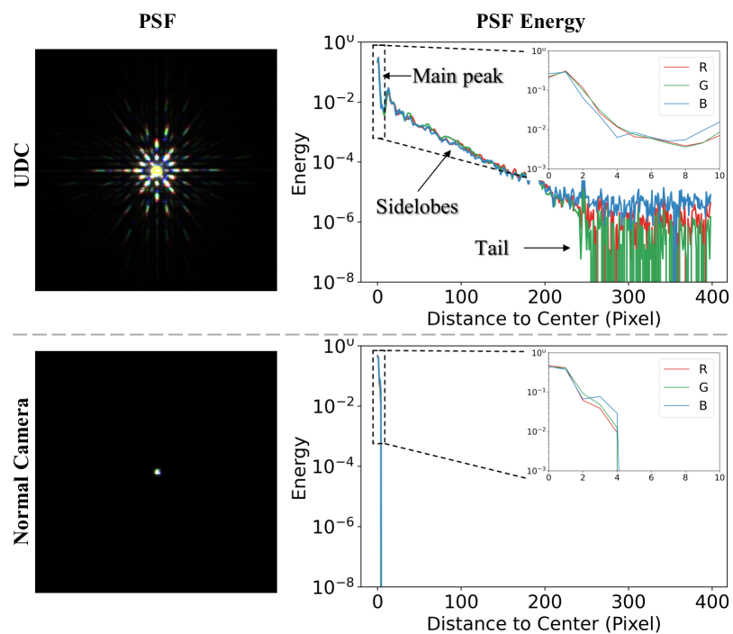
Figure 3: Comparison of PSF energy for UDC and normal camera. The PSF is brightened to visualize the structured sidelobe patterns. Due to the finite aperture size and manufacturing imperfections, the PSF of a real normal camera (Bottom left) will be a blur kernel of some size, rather than a perfect point.

3.2 PSF Measurement

In Figure 2, the optical field $U_{S}(p,q)$ captured by the sensor given a unit amplitude point source input can be expressed as

$$U_{S}(p,q)= \left\{\left[\exp\left({\frac{i\pi r^{2}}{\lambda z_{1}}}\right)\cdot t(p,q)\right]*\exp\left({\frac{i\pi r^{2}}{\lambda d}}\right)\right.$$ (2)

$$\left.\cdot\exp\left({\frac{-i\pi r^{2}}{\lambda f}}\right)\right\}*\exp\left({\frac{i\pi r^{2}}{\lambda z_{2}}}\right).$$

Here, $(p,q)$ is the 2D spatial coordinates, $r^{2}=p^{2}+q^{2}$, $\lambda$ is the wavelength, $f$ is the focal length of the lens, $t(p,q)$ is the transmission function of the display. $z_{1}$, $d$ and $z_{2}$ denote the distance between the light source and the display, the distance between the display and the lens, and the distance between the lens and the sensor, respectively. $*$ denotes the convolution, and $\cdot$ denotes multiplication. Finally, the PSF of the imaging system is given by $k=|U_{S}|^{2}$.

With the exact pixel layout of a certain display, we can theoretically simulate the PSF of an optical system modulated by the display. However, we found that although the simulated and real-measured PSF share a similar shape, they slightly differ in color and contrast due to model approximations and manufacturing imperfections (see Supplement for light propagation model and simulated PSF). Besides, we have no access to the transmission function $t(p,q)$ for the OLED display we used in this work, whose pixel structure is unknown due to proprietary reasons.

Therefore, we follow [31] and devise an imaging system to directly measure the PSF by placing a white point light source $1$-meter away from the OLED display. At this distance, the size of the point light source is equivalent to one pixel of the sensor. Hence, this illuminant can be considered as an impulse input. To capture the entire PSF, including the strong main peak and the weak sidelobes, we take three images successively at different exposures: [$1$, $1/32$, $1/768$], which are then normalized to the same brightness level. Subsequently we pick out all unsaturated pixel values to fuse into one HDR image. The captured PSF of the UDC system (Figure 3 top) shows structured patterns: 1) the response at the center, denoted as main peak, is very strong and has greater energy with an order of magnitude. 2) Compared to the PSF of a normal camera, it has larger spatial support (over $800\times 800$) and spike-shaped long-tail sidelobes whose energy decreases exponentially. 3) In the tail regions of the sidelobe, we can an observe obvious color shift. To summarize, the PSF of UDC has several special characteristics compared to regular blur kernel, which motivates a simulation based on HDR images.

Compared with the UDC image formation model described in [47], our model is closer to the real situation in the following two aspects. First, the objects $x$ that we considered are real scenes with high dynamic range. Since the PSF of UDC has a strong response at the center but vastly lower energy at long-tail sidelobes, only when convolved with sufficiently high-intensity scenes, these spike-shaped sidelobes can be amplified to be visible (flares) in the degraded image. Hence, images captured by UDC systems in real scenes will exhibit structured flares near strong light sources. The imaging system in [47], however, cannot model this degradation, because it captures images displayed on an LCD monitor, which commonly has limited dynamic range. We demonstrate in Supplement that if we clip the same scene from high dynamic range to low dynamic range, these flares caused by diffraction become invisible. Second, due to the high dynamic range of the input scene, the digital sensor (usually 10-bit) will inevitably get saturated in real applications, resulting in an information loss. This factor should be considered in the image formation model as well.

3.3 Data Collection and Simulation

Simulated Data. To generate the synthetic data, we gathered $132$ HDR images with large dynamic ranges from HDRI Haven dataset. Each HDR panorama image is a 360-degree panorama of resolution $8192\times 4096$. We first re-projected these panorama images back to perspective view and then cropped them into $800\times 800$ patches. In this way, we got a total of $2016$ subimages for training and $360$ for testing. For each of the crops, we simulated the corresponding degraded image using Eqn. 1, where the PSF calibrated in Section 3.2 is used as the kernel $k$. Refer to the Supplemental Material for more details.

Real Data. For each real scene, we captured three images of different exposures: [$1$, $1/4$, $1/16$] using ZTE Axon 20 phone, and then combine them into one HDR image. To ensure the linearity of the data, we directly used the raw data after HDR fusion, without any non-linear processing.

4 Dynamic Skip Connection Network

4.1 Motivation

We treat UDC image restoration as a non-blind image restoration problem, where a degraded image $\{\hat{y}_{i}\}$ and the ground-truth degradation (PSF) $\{k_{i}\}$ are given to restore the clear image $\{x_{i}\}$. In general, with the known convolution kernel, non-blind restoration establishes the upper bound for blind restoration, where the kernel needs to be estimated. Despite claiming our method as non-blind, we note that it can be used towards blind UDC image restoration by incorporating any PSF estimation algorithm.

Traditionally, non-blind image restoration is solved by classical deconvolution, e.g., Wiener filter [20], which have a rigorous assumption on the linearity of the system. UDC artifacts occur in HDR scenes, where the sensor is over-saturated in high-intensity area, breaking the linearity of the system and losing the information within. Additionally, traditional deconvolution do not consider extremely large kernels ($800\times 800$), thus causing serious ringing and halo artifacts (Figure 5 and Figure 6). Moreover, deep learning-based methods could leverage more data to learn restoration and require only one forward pass during inference. In this regard, we use a network to reconstruct $\hat{x}_{i}=\phi(x_{i})$, which suggests a recovery from $\hat{y}$ to $\hat{x}$ in the non-linear tone-mapped domain, yielding triplet set $\{\hat{y}_{i},k_{i},\hat{x}_{i}\}$. Such optimization in the tone-mapped domain gives more emphasis to darker pixels and encourages the balance of restoration in different regions.

Moreover, the image formation model in Eqn. 1 assumes a shift-invariant 2-D convolution. Now in the tone-mapped domain with non-linear sensor saturation, such assumption no longer holds, since the PSF’s shape and intensity can be variant based on the input pixel and its neighborhood at the corresponding location. For example, the OLED diffracting saturated highlights into neighboring unsaturated areas motivates an adaptive recovery of clipped information from the nearby areas. Inspired by recent success of Kernel Prediction Network (KPN) [9, 17, 18, 45], we propose DynamIc Skip Connection Network (DISCNet), which dynamically generates filter kernel at each pixel and applies them to different feature spaces at different network layers with skip connections. This network is conditioned on two inputs: 1) the PSF that provides domain knowledge about the image formation model, and 2) the degraded image that provides light intensity and neighborhood context information to facilitate a spatially-variant recovery. We demonstrate the effectiveness of the coupled conditions in Section 5.2.

For dynamic convolution, directly applying the predicted filters in the image domain like most existing KPN-based approaches is not best suited for UDC image restoration, because the PSF in UDC has large support and long-tail side lobes (see Figure 3). As discussed in [37], such an inverse convolution process with a large PSF can only be well approximated in image domain with sufficiently large kernels (larger than $100$), while the size of dynamic filters is typically far smaller (e.g.$5$ or $7$). Therefore, we propose to apply dynamic convolution in the feature domain. On top of that, we construct a multi-scale architecture, where the filter generator at each scale predicts dynamic filters separately, to further enlarge the spatial support of the learned filters.

4.2 Network Architecture

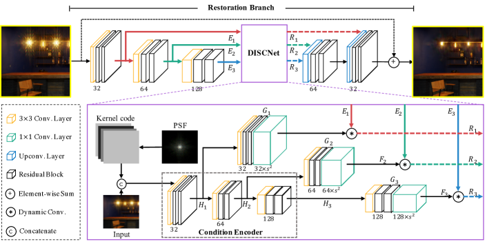
Figure 4: Illustration of the proposed DISCNet. The main restoration branch consists of an encoder and a decoder, with feature maps propagated and transformed by DISCNet through skip connections. DISCNet applies multi-scale dynamic convolutions using generated filters conditioned on PSF kernel code and spatial information from input images.

As shown in Figure 4, our network comprises a restoration branch and a DynamIc Skip Connection Network (DISCNet). The restoration branch learns to extract features and restore the final clean image. DISCNet is employed to tackle various degradations and transform and refine the features extracted from the restoration branch.

Training with Various Degradations. Suppose the degraded image $\hat{y}_{i}$ is of shape $H\times W\times C$, where $H$, $W$, $C$ denote the height, width, and the number of channels of images. Following [5], we project the PSF onto a $b$-dimensional vector, referred to as kernel code, by Principal Component Analysis (PCA) to reduce computational complexities. The kernel code is then stretched into degradation maps of size $H\times W\times b$ and concatenated with the degraded image to get the condition maps of size $H\times W\times(b+C)$ , which are then fed into the DISCNet. In this paper, we empirically set $b=5$.

Restoration Branch. This branch builds upon an encoder-decoder architecture with skip connections to restore the degraded images. Specifically, the encoder contains three convolutional blocks, each of which has a $3\times 3$ convolution layer with stride $2$, a LeakyReLU [6] layer, and two residual blocks [7], extracting features $E_{1}$, $E_{2}$, $E_{3}$ at three different scales. The extracted features are fed into DISCNet and transformed into $R_{1}$, $R_{2}$, $R_{3}$, respectively. Similarly, the decoder consists of two convolutional blocks, including an up-convolution layer and two residual blocks. Each convolutional block takes the transformed feature at its corresponding scale as input and reconstructs the final tone-mapped sharp images.

DynamIc Skip Connection Network. The proposed DISCNet mainly consists of three designs: condition encoder, multi-scale filter generator, dynamic convolution.

Given the condition maps as input, the condition encoder extracts scale-specific feature maps $H_{1}$, $H_{2}$, $H_{3}$ using $3$ blocks similar to the encoder of the restoration branch. Although the kernel code maps are globally uniform, the condition encoder could still capture rich information from the degraded image with spatial variability and manage to recover saturated information from nearby low-light regions.

Then, the extracted features at different scales are fed into their corresponding filter generators, where each comprises a $3\times 3$ convolution layer, two residual blocks, and a $1\times 1$ convolution layer to expand feature dimension. Particularly, given the size of dynamic filters $s$, a filter generator $G_{n}$ takes in the extracted feature maps at a specific scale $H_{n}\in\mathbb{R}^{h\times w\times c}$ and outputs predicted filters $F_{n}=G_{n}(H_{n})$, where the generated filters $F_{n}$ is of size $h\times w\times cs^{2}$. The filters are then used by a dynamic convolution to refine features $E_{n}$. For each pixel $(i,j,c_{m})$ of features $E_{n}\in h\times w\times c$, the output feature $R_{n}$ is given by

$$R_{n}(i,j,c_{m})=\langle K_{n}(i,j,c_{m}),\varphi(E_{n}(i,j,c_{m}))\rangle,$$ (3)

where $K_{n}(i,j,c_{m})$ is a $s\times s$ filter reshaped from $F_{n}(i,j,c_{m})\in\mathbb{R}^{1\times 1\times s^{2}}$. $\varphi(\cdot)$ denotes a $s\times s$ patch centered at position $(i,j,c_{m})$, and $\langle\cdot\rangle$ represents inner product. The refined feature $R_{n}$ is then cast to the restoration branch.

5 Experiments

Table 1: Ablation results on the simulated dataset. Starting from the baseline model, we gradually add each component in our network to validate their effectiveness. “*” indicates results evaluated on the simulation over single PSF. The best results are highlight.

Method	PSF	Filter Generators	Conditions	PSNR*	$\text{PSNR}_{avg}$	SSIM*	$\text{SSIM}_{avg}$
(a) Baseline on $1$ kernel	Single	-	-	$41.47$	$38.55$	$0.9850$	$0.9742$
(b) Baseline on various kernels	Variational	-	-	$40.67$	$40.87$	$0.9823$	$0.9833$
(c) w/ image conditions	Variational	Single-scale	Image	$41.33$	$41.59$	$0.9842$	$0.9851$
(d) w/ PSF conditions	Variational	Single-scale	PSF	$41.95$	$42.14$	$0.9848$	$0.9857$
(e) w/ image & PSF conditions	Variational	Single-scale	Image + PSF	$42.60$	$42.77$	$0.9861$	$0.9870$
(f) DISCNet (Ours)	Variational	Multi-scale	Image + PSF	$\mathbf{43.06}$	$\mathbf{43.27}$	$\mathbf{0.9870}$	$\mathbf{0.9877}$

5.1 Implementation Details

Datasets. We train the proposed model with the synthetic triplet data. To evaluate the effectiveness of DISCNet for non-blind degradations, we consider rotating PSF, which is analogous to rotating the display around the optical axis in imaging systems. To account for variations in the rotation angle, we build a kernel set in which the angles vary within $(-12,12)$ where $0$ radian refers to the original PSF. Under this setting, each degraded image $\hat{y}_{i}$ is simulated using Eqn. 1, with the convolution kernel $k_{i}$ is uniformly sampled from the kernel set. During training, the subimages are randomly cropped into $256\times 256$ patches. More details about simulation settings can be found in Supplement Material.

Training Setups. We initialize all networks with Kaiming Normal [6] and train them using Adam optimizer [12] with $\beta_{1}=0.9$, $\beta_{2}=0.999$ and $\theta=10^{-8}$ to minimize a weighted combination of $\mathcal{L}_{1}$ loss and VGG loss [11]. The mini-batch size for all the experiments is set to 16. The learning rate is decayed with a cosine annealing schedule, where $\eta_{min}=1\times 10^{-7}$, $\eta_{max}=2\times 10^{-4}$, and is restarted every $2\times 10^{5}$ iterations. For all experiments, we implement our models with the PyTorch [21] framework and train them using 2 NVIDIA V100 GPUs.

5.2 Ablation Study

In this subsection, we analyze the effectiveness of each component in DISCNet. The baseline methods (Table 1(a) and (b)) strip DISCNet in Figure 4. In this case, the restoration branch reduces to a variant of UNet architecture [26], and $E_{1}$, $E_{2}$, $E_{3}$ are equivalent to $R_{1}$, $R_{2}$, $R_{3}$, respectively. Then we gradually apply different filter generators and condition maps for ablation studies. We report PSNR, SSIM, and LPIPS [43] as the evaluation metrics. The FLOPs is calculated by input size of $800\times 800\times 3$.

Learning Variational Degradations. Comparing Table 1(a) and Table 1(b), we found that our baseline trained on a dataset with only $1$ kernel can easily overfit to single degraded dataset but fails to generalize to other degradation types. In particular, the performance deteriorates seriously across other datasets, due to the discrepancy between the assumed PSF and real ones.

Type of Conditions. On top of the baseline network, we first investigate a single-scale variant of our network, i.e., removing filter generators $G_{1}$ and $G_{2}$ from Figure 4. As a result, feature $E_{1}$ and $E_{2}$ remain unchanged and are cast back to restoration branch via skip connections. By applying different types of conditions, we observe a significant improvement on average PSNR over the baselines. For example, model with image condition (Table 1(c)) and the one with the PSF condition (Table 1(d)) improve $0.72$ dB and $1.27$ dB, respectively. Besides, combining both PSF and image conditions (Table 1(e)) brings additional improvements ($1.18$/$0.63$ dB increase on PSF/image conditions). This indicates even the simplest single-scale dynamic convolution design could benefit the feature refinement.

Single-scale vs.Multi-scale. By applying multi-scale dynamic filter generators to transform skip connections at all scale, our proposed DISCNet (Table 1(f)) increase $0.5$ dB over its single-scale counterpart (Table 1(e)). This demonstrates the effectiveness of multi-scale strategy.

Size of Dynamic Filters. To further investigate the best trade-offs between performance and model size, we vary the size of dynamic filters. As shown in Table 2, larger size of filters can bring better performance. However, the performance become even worse by increasing size after $s=5$, while the amount of parameters significantly increases. Hence, we empirically choose $s=5$ by default.

Table 2: Results over different sizes of dynamic filters.

Filter Size	$s=3$	$s=5$	$s=7$	$s=9$
PSNR	$42.16$	$42.77$	$42.62$	$42.47$
SSIM	$0.9862$	$0.9870$	$0.9869$	$0.9868$
LPIPS [43]	$0.0126$	$0.0119$	$0.0119$	$0.0119$
Params (M)	$3.18$	$3.44$	$3.84$	$4.37$
FLOPs (G)	$262.10$	$272.59$	$288.32$	$309.29$

5.3 Evaluation on Simulated Dataset

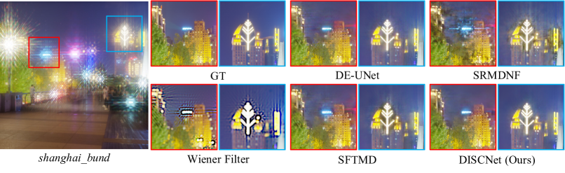
Figure 5: Visual comparison on a synthetic input image. Our method restores fine details and suppresses flare effects in both highlight and dark regions and renders visually pleasing results. Refer to Supplement for more visual results. Zoom in for better view.

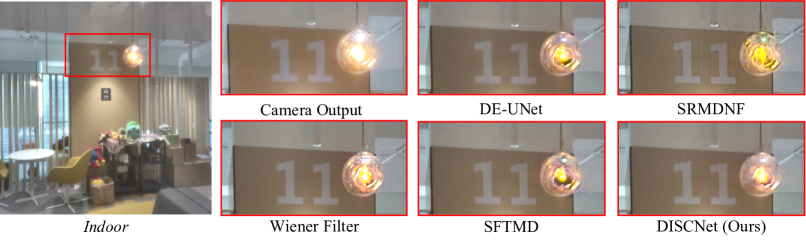
Figure 6: Visual comparison on a real input image. Our method achieves the best perceptual quality while other approaches leave noticeable artifacts and suffer from strong noise. Refer to Supplement for more visual results. Zoom in for better view.

To demonstrate the efficiency of DISCNet, we conduct experiments to evaluate the performance on simulated dataset. Since UDC image restoration is a newly-defined problem, we carefully select and modify four representative and state-of-the-art non-blind image restoration algorithms as baselines: Wiener Filter [20] is a classical deconvolution algorithm for linear convolution formation. Hence, we apply Wiener deconvolution to the degraded images with measured PSF $k$ for each channel independently in the linear domain. Note that the restored images are still evaluated and displayed in tone-mapped domain. SRMDNF [42] is a noise-free version of SRMD, which integrates non-blind degradation information to handle multiple degradations in a super-resolution network. The network contains $12$ convolution layers, each of which produces $128$ feature maps. By conventions of network designed for low-level tasks [35, 15], we remove BN layers to stabilize the training. SFTMD [5]. Iterative Kernel Correction (IKC) is originally devised for image super-resolution on blind setting. In our experiments, we employ SFTMD network which also leverages the kernel information to solve the non-blind problem. We remove the pixel shuffle upsampling layer as the input and output share the same shape in UDC restoration task. DE-UNet [47]. Zhou et al.presents a Double-Encoder UNet, referred to as DE-UNet in our experiments, to recover UDC degraded images. We modify the first layers of two encoders to take $3$-channel RGB images as inputs.

Table 3: Quantitative comparison on the simulated dataset. “*” indicates blind models that do not explicitly use the information of kernel. The best two results are highlighted in red and blue.

Method	Params (M)	FLOPs (G)	PSNR	SSIM	LPIPS
WF [20]	-	-	$27.41$	$0.8392$	$0.3365$
SRMDNF [42]	$1.49$	$951$	$34.80$	$0.9659$	$0.0360$
DE-UNet* [47]	$9.02$	$169$	$39.81$	$0.9795$	$0.0206$
SFTMD [5]	$3.85$	$2460$	$42.35$	$0.9863$	$0.0123$
DISCNet	$3.80$	$364$	$43.27$	$0.9877$	$0.0108$

Quantitative Comparisons. For all deep learning-based methods, we train them using the same training settings and data. Table 3 shows quantitative results on simulated dataset. The proposed algorithm performs favorably against other baseline methods. We observe that the proposed DISCNet consistently outperforms all other approaches on the simulated dataset. Even with the exact PSF kernel, Wiener Filter [20] only achieves low image quality far below that of deep learning-based methods. SRMDNF [42] builds upon a plain network and uses a simple strategy to utilize the kernel information. Therefore, it cannot adapt to degraded regions caused by highlight sources and produces inferior results. Compared to SFTMD [5], our network could achieve better performance with only $15\%$ computational cost (decline from $2459.57$ to $364.34$ GFLOPs). This suggests DISCNet is efficient and particularly fit for this task, while any other boiler-plate network (e.g., plain net, UNet) produces unsatisfactory results.

Visual Comparisons. Figure 5 compares the proposed model with existing methods on simulated dataset. As one can see, Wiener filter produces unpleasing results and suffers from serious ringing and halo artifacts. In comparison, our DISCNet generates the most perceptually pleasant results and removes diffraction artifacts derived from highlights in the unsaturated regions. The presented visual results in Figure Removing Diffraction Image Artifacts in Under-Display Camera via Dynamic Skip Connection Network and Figure 5 and additional results in the Supplemental Material validate the performance of the proposed DISCNet for various scene types, e.g., night-time urban scenes and indoor settings with strong light sources.

5.4 Evaluation on Real Dataset

Apart from the evaluation on synthetic dataset, this section explores reconstruction performance on real dataset. Since the ground-truth images are inaccessible, we provide the qualitative comparisons as shown in Figure 6. We also include the camera output of ZTE phone for comparisons. As the real data is captured without ISP, we adopt simple post-processing to all outputs except camera output for better visualization. Our network achieves the best perceptual quality while other approaches leave noticeable artifacts and suffer from strong noise or flare. Post-processing and more visual results can be found in Supplement.

6 Discussion

Limitations. Our work is only the first step towards removing diffraction image artifacts in UDC systems. Other complexities, e.g., spatially-varying PSF, noise in low light, and defocus, require more study. The proposed DISCNet sometimes will fail due to the domain gap between simulated and real data, e.g., camera noise, motion blur, variations in scenes. Our method currently is also too heavy-weight. See Supplement for further discussion and failure cases.

Conclusion. In this paper, we define a physics-based image formation model and measure the real-world PSF of the UDC system, and provide a model-based data synthesis pipeline to generate realistically degraded images. Then, we propose a new domain knowledge-enabled Dynamic Skip Connection Network (DISCNet) to restore the UDC images. We offer a foundation for further exploration in UDC image restoration. Our perspective on UDC has potential to inspire more diffraction-limited image restoration work.

Acknowledgements. Thanks Joshua Rego and Guiqi Xiao for assistance on data collection. This research was conducted in collaboration with SenseTime. This work is supported by A*STAR through the Industry Alignment Fund - Industry Collaboration Projects Grant.

References

- [1] M Salman Asif, Ali Ayremlou, Aswin Sankaranarayanan, Ashok Veeraraghavan, and Richard G Baraniuk. Flatcam: Thin, lensless cameras using coded aperture and computation. IEEE Transactions on Computational Imaging, 3(3):384–397, 2016.
- [2] Steve Bako, Thijs Vogels, Brian McWilliams, Mark Meyer, Jan Novák, Alex Harvill, Pradeep Sen, Tony Derose, and Fabrice Rousselle. Kernel-predicting convolutional networks for denoising monte carlo renderings. ACM Trans. Graph., 36(4):97–1, 2017.
- [3] Sefi Bell-Kligler, Assaf Shocher, and Michal Irani. Blind super-resolution kernel estimation using an internal-gan. In Advances in Neural Information Processing Systems, pages 284–293, 2019.
- [4] Sunghyun Cho, Jue Wang, and Seungyong Lee. Handling outliers in non-blind image deconvolution. In 2011 International Conference on Computer Vision, pages 495–502. IEEE, 2011.
- [5] Jinjin Gu, Hannan Lu, Wangmeng Zuo, and Chao Dong. Blind super-resolution with iterative kernel correction. In Proceedings of the IEEE Conference on Computer Vision and Pattern Recognition, pages 1604–1613, 2019.
- [6] Kaiming He, Xiangyu Zhang, Shaoqing Ren, and Jian Sun. Delving deep into rectifiers: Surpassing human-level performance on imagenet classification. In Proceedings of the IEEE international conference on computer vision, pages 1026–1034, 2015.
- [7] Kaiming He, Xiangyu Zhang, Shaoqing Ren, and Jian Sun. Deep residual learning for image recognition. In Proceedings of the IEEE conference on computer vision and pattern recognition, pages 770–778, 2016.
- [8] Matthew Hirsch, Douglas Lanman, Henry Holtzman, and Ramesh Raskar. Bidi screen: a thin, depth-sensing lcd for 3d interaction using light fields. ACM Transactions on Graphics (ToG), 28(5):1–9, 2009.
- [9] Xu Jia, Bert De Brabandere, Tinne Tuytelaars, and Luc V Gool. Dynamic filter networks. In Advances in neural information processing systems, pages 667–675, 2016.
- [10] Younghyun Jo, Seoung Wug Oh, Jaeyeon Kang, and Seon Joo Kim. Deep video super-resolution network using dynamic upsampling filters without explicit motion compensation. In Proceedings of the IEEE conference on computer vision and pattern recognition, pages 3224–3232, 2018.
- [11] Justin Johnson, Alexandre Alahi, and Li Fei-Fei. Perceptual losses for real-time style transfer and super-resolution. In European conference on computer vision, pages 694–711. Springer, 2016.
- [12] Diederik P. Kingma and Jimmy Ba. Adam: A method for stochastic optimization. CoRR, abs/1412.6980, 2015.
- [13] Hyeok-Jun Kwon, Chang-Mo Yang, Min-Cheol Kim, Choon-Woo Kim, Ji-Young Ahn, and Pu-Reum Kim. Modeling of luminance transition curve of transparent plastics on transparent oled displays. Electronic Imaging, 2016(20):1–4, 2016.
- [14] Anat Levin, Yair Weiss, Fredo Durand, and William T Freeman. Understanding and evaluating blind deconvolution algorithms. In 2009 IEEE Conference on Computer Vision and Pattern Recognition, pages 1964–1971. IEEE, 2009.
- [15] Bee Lim, Sanghyun Son, Heewon Kim, Seungjun Nah, and Kyoung Mu Lee. Enhanced deep residual networks for single image super-resolution. In Proceedings of the IEEE conference on computer vision and pattern recognition workshops, pages 136–144, 2017.
- [16] Sehoon Lim, Yuqian Zhou, Neil Emerton, Lincoln Ghioni, Tim Large, and Steven Bathiche. Camera in display, 2020 (accessed Nov. 9, 2020). https://www.microsoft.com/applied-sciences/projects/camera-in-display.
- [17] Ben Mildenhall, Jonathan T Barron, Jiawen Chen, Dillon Sharlet, Ren Ng, and Robert Carroll. Burst denoising with kernel prediction networks. In Proceedings of the IEEE Conference on Computer Vision and Pattern Recognition, pages 2502–2510, 2018.
- [18] Simon Niklaus, Long Mai, and Feng Liu. Video frame interpolation via adaptive convolution. In Proceedings of the IEEE Conference on Computer Vision and Pattern Recognition, pages 670–679, 2017.
- [19] Simon Niklaus, Long Mai, and Feng Liu. Video frame interpolation via adaptive separable convolution. In Proceedings of the IEEE International Conference on Computer Vision, pages 261–270, 2017.
- [20] François Orieux, Jean-François Giovannelli, and Thomas Rodet. Bayesian estimation of regularization and point spread function parameters for wiener–hunt deconvolution. JOSA A, 27(7):1593–1607, 2010.
- [21] Adam Paszke, Sam Gross, Soumith Chintala, Gregory Chanan, Edward Yang, Zachary DeVito, Zeming Lin, Alban Desmaison, Luca Antiga, and Adam Lerer. Automatic differentiation in pytorch. 2017.
- [22] Yifan Peng, Qilin Sun, Xiong Dun, Gordon Wetzstein, Wolfgang Heidrich, and Felix Heide. Learned large field-of-view imaging with thin-plate optics. ACM Trans. Graph., 38(6):219–1, 2019.
- [23] Zong Qin, Yu-Hsiang Tsai, Yen-Wei Yeh, Yi-Pai Huang, and Han-Ping David Shieh. See-through image blurring of transparent organic light-emitting diodes display: calculation method based on diffraction and analysis of pixel structures. Journal of Display Technology, 12(11):1242–1249, 2016.
- [24] Zong Qin, Jing Xie, Fang-Cheng Lin, Yi-Pai Huang, and Han-Ping D Shieh. Evaluation of a transparent display’s pixel structure regarding subjective quality of diffracted see-through images. IEEE Photonics Journal, 9(4):1–14, 2017.
- [25] William Hadley Richardson. Bayesian-based iterative method of image restoration. JoSA, 62(1):55–59, 1972.
- [26] Olaf Ronneberger, Philipp Fischer, and Thomas Brox. U-net: Convolutional networks for biomedical image segmentation. In International Conference on Medical image computing and computer-assisted intervention, pages 234–241. Springer, 2015.
- [27] Christian J Schuler, Harold Christopher Burger, Stefan Harmeling, and Bernhard Scholkopf. A machine learning approach for non-blind image deconvolution. In Proceedings of the IEEE Conference on Computer Vision and Pattern Recognition, pages 1067–1074, 2013.
- [28] Assaf Shocher, Nadav Cohen, and Michal Irani. “zero-shot” super-resolution using deep internal learning. In Proceedings of the IEEE Conference on Computer Vision and Pattern Recognition, pages 3118–3126, 2018.
- [29] Sungjoo Suh, Changkyu Choi, Dusik Park, and Changyeong Kim. 50.2: Adding depth-sensing capability to an oled display system based on coded aperture imaging. In SID Symposium Digest of Technical Papers, volume 44, pages 697–700. Wiley Online Library, 2013.
- [30] Sungjoo Suh, Changkyu Choi, Kwonju Yi, Dusik Park, and Changyeong Kim. P-135: An lcd display system with depth-sensing capability based on coded aperture imaging. In SID Symposium Digest of Technical Papers, volume 43, pages 1574–1577. Wiley Online Library, 2012.
- [31] Qilin Sun, Ethan Tseng, Qiang Fu, Wolfgang Heidrich, and Felix Heide. Learning rank-1 diffractive optics for single-shot high dynamic range imaging. In The IEEE Conference on Computer Vision and Pattern Recognition (CVPR), June 2020.
- [32] Quan Tang, He Jiang, Xindong Mei, Shaojun Hou, Guanghui Liu, and Zhifu Li. 28-2: Study of the image blur through ffs lcd panel caused by diffraction for camera under panel. In SID Symposium Digest of Technical Papers, volume 51, pages 406–409. Wiley Online Library, 2020.
- [33] Jiaqi Wang, Kai Chen, Rui Xu, Ziwei Liu, Chen Change Loy, and Dahua Lin. Carafe: Content-aware reassembly of features. In Proceedings of the IEEE International Conference on Computer Vision, pages 3007–3016, 2019.
- [34] Xintao Wang, Ke Yu, Chao Dong, and Chen Change Loy. Recovering realistic texture in image super-resolution by deep spatial feature transform. In Proceedings of the IEEE Conference on Computer Vision and Pattern Recognition, pages 606–615, 2018.
- [35] Xintao Wang, Ke Yu, Shixiang Wu, Jinjin Gu, Yihao Liu, Chao Dong, Yu Qiao, and Chen Change Loy. Esrgan: Enhanced super-resolution generative adversarial networks. In Proceedings of the European Conference on Computer Vision (ECCV), pages 0–0, 2018.
- [36] Oliver Whyte, Josef Sivic, and Andrew Zisserman. Deblurring shaken and partially saturated images. International journal of computer vision, 110(2):185–201, 2014.
- [37] Li Xu, Jimmy SJ Ren, Ce Liu, and Jiaya Jia. Deep convolutional neural network for image deconvolution. In Advances in neural information processing systems, pages 1790–1798, 2014.
- [38] Xiangyu Xu, Muchen Li, and Wenxiu Sun. Learning deformable kernels for image and video denoising. arXiv preprint arXiv:1904.06903, 2019.
- [39] Yu-Syuan Xu, Shou-Yao Roy Tseng, Yu Tseng, Hsien-Kai Kuo, and Yi-Min Tsai. Unified dynamic convolutional network for super-resolution with variational degradations. In Proceedings of the IEEE/CVF Conference on Computer Vision and Pattern Recognition, pages 12496–12505, 2020.
- [40] Yuan Yuan, Siyuan Liu, Jiawei Zhang, Yongbing Zhang, Chao Dong, and Liang Lin. Unsupervised image super-resolution using cycle-in-cycle generative adversarial networks. In Proceedings of the IEEE Conference on Computer Vision and Pattern Recognition Workshops, pages 701–710, 2018.
- [41] Jiawei Zhang, Jinshan Pan, Wei-Sheng Lai, Rynson WH Lau, and Ming-Hsuan Yang. Learning fully convolutional networks for iterative non-blind deconvolution. In Proceedings of the IEEE Conference on Computer Vision and Pattern Recognition, pages 3817–3825, 2017.
- [42] Kai Zhang, Wangmeng Zuo, and Lei Zhang. Learning a single convolutional super-resolution network for multiple degradations. In IEEE Conference on Computer Vision and Pattern Recognition, volume 6, 2018.
- [43] Richard Zhang, Phillip Isola, Alexei A Efros, Eli Shechtman, and Oliver Wang. The unreasonable effectiveness of deep features as a perceptual metric. In Proceedings of the IEEE conference on computer vision and pattern recognition, pages 586–595, 2018.
- [44] Ruofan Zhou and Sabine Susstrunk. Kernel modeling super-resolution on real low-resolution images. In Proceedings of the IEEE International Conference on Computer Vision, pages 2433–2443, 2019.
- [45] Shangchen Zhou, Jiawei Zhang, Jinshan Pan, Haozhe Xie, Wangmeng Zuo, and Jimmy Ren. Spatio-temporal filter adaptive network for video deblurring. In Proceedings of the IEEE International Conference on Computer Vision, pages 2482–2491, 2019.
- [46] Yuqian Zhou, Michael Kwan, Kyle Tolentino, Neil Emerton, Sehoon Lim, Tim Large, Lijiang Fu, Zhihong Pan, Baopu Li, Qirui Yang, et al. Udc 2020 challenge on image restoration of under-display camera: Methods and results. In European Conference on Computer Vision, pages 337–351. Springer, 2020.
- [47] Yuqian Zhou, David Ren, Neil Emerton, Sehoon Lim, and Timothy Large. Image restoration for under-display camera. arXiv preprint arXiv:2003.04857, 2020.