A dynamical measurement of the disk mass in Elias 2-27

Abstract

Recent multi-wavelength ALMA observations of the protoplanetary disk orbiting around Elias 2-27 revealed a two armed spiral structure. The observed morphology together with the young age of the star and the disk-to-star mass ratio estimated from dust continuum emission make this system a perfect laboratory to investigate the role of self-gravity in the early phases of star formation. This is particularly interesting if we consider that gravitational instabilities could be a fundamental first step for the formation of planetesimals and planets. In this Letter, we model the rotation curve obtained by CO data of Elias 2-27 with a theoretical rotation curve including both the disk self-gravity and the star contribution to the gravitational potential. We compare this model with a purely Keplerian one and with a simple power-law function. We find that (especially for the ¹³CO isotopologue) the rotation curve is better described by considering not only the star, but also the disk self-gravity. We are thus able to obtain for the first time a dynamical estimate of the disk mass of $0.08\pm 0.04\,M_{\odot}$ and the star mass of $0.46\pm 0.03\,M_{\odot}$ (in the more general case), the latter being comparable with previous estimates. From these values, we derive that the disk is 17$\%$ of the star mass, meaning that it could be prone to gravitational instabilities. This result would strongly support the hypothesis that the two spiral arms are generated by gravitational instabilities.

1 Introduction

Protoplanetary disks form in the chaotic environment of molecular cloud cores and in their early stages they are massive enough to have a non negligible effect on the evolution of the overall system. The disk self-gravity may influence the disk dynamics through the propagation of density waves that lead to the formation of prominent structures in the form of one or more spiral arms. These morphologies have been detected by ALMA and VLT-SPHERE in both Class 0/I and Class II systems, and they are usually assumed to be originated by embedded companions (e.g. HD135344B, Veronesi et al. 2019, MWC 758, Calcino et al. 2020) or by self-gravity (e.g. Elias 2-27, Pérez et al. 2016; Huang et al. 2018a). In the second case, density waves are thought to provide a non negligible contribution to the angular momentum transport and may have a crucial role in the formation of planetesimals through dust trapping at the location of the spirals and the following direct fragmentation of spiral overdensities into bound objects (Rice et al., 2004, 2006; Kratter & Lodato, 2016). Being able to give an estimate of the disk mass is the first step in order to put other pieces in the puzzle of planet formation and to understand the origin of the observed spirals (van der Marel et al., 2020; Veronesi et al., 2019; Bergin & Williams, 2018). But how can we determine the mass of these systems?

First, dust masses are typically inferred using the optically thin approximation at millimeter wavelengths. It is worth noting that, although it may be trivial, this estimate still carries a high level of uncertainty, due to the assumed optical depth of the dust at (sub-)mm wavelengths (e.g. the dust opacity and the level of dust growth, Bergin & Williams 2018). Once the dust mass is known, one needs to convert this into a total disk mass by assuming some gas/dust ratio, which is generally assumed to be equal to 100 (Draine, 2003), although this number is highly uncertain (see e.g. Macias et al. 2021). On the other hand, it is more difficult to quantify the disk mass from direct gas tracers. A common procedure is to use CO observations in its various isotopologues (such as ¹³CO and C¹⁸O) as a proxy for the gas mass. But since the conversion of the observed CO mass into total gas mass is not well understood (Williams & Best, 2014; Bergin & Williams, 2018), this is not straightforward. Another issue adding complexity to the problem is that the properties of different molecules also vary spatially and temporally, depending on the models (Ilee et al., 2017; Quénard et al., 2018). Indeed, estimates derived from CO observations result in very low disk masses compared to dust estimates (Pascucci et al., 2016; Ansdell et al., 2016; Miotello et al., 2017; Long et al., 2017). Miotello et al. (2016) associated this trend with multiple possible processes: carbon depletion in the disk (Favre et al., 2013; Bosman et al., 2018; Cleeves et al., 2018), photodissociation in the upper layers, freeze-out at the disk midplane or in general other isotope-selective processes. Another aspect that should be considered comes from far-IR HD lines (Bergin et al., 2013; Trapman et al., 2017) observations, suggesting that the gas-to-dust ratio measurement is affected by the fact that the emitting regions of various gas tracers differ from each other and in turn differ from the regions where the dust is observed.

We can also estimate the total disk mass in a dynamical way, by using the disk rotation curve, and detecting deviations from the expected Keplerian curve. This method has been widely used with galaxies (Barbieri et al., 2005) and sometimes it has been used to estimate also the mass of AGN disks (Lodato & Bertin, 2003). Usually protoplanetary disks are assumed to be Keplerian, since typically the stellar mass dominates over the disk mass, and their rotation curve can be sufficiently well described by the stellar contribution alone. Instead, when the disk contribution is significant, we could be able to fit the observed rotation curve and to give an independent disk mass estimate (Bertin & Lodato, 1999). For relatively massive disks, this dynamical estimate is now possible since we have access to a large amount of gas kinematic data with high (angular and velocity) resolution and high sensitivity. From these data, we can infer the geometry of the disk and recover the height and the velocity of the emitting gas layer (Pinte et al., 2018).

One of the most interesting observed spiral structures is the one hosted by the protoplanetary disk orbiting around Elias 2-27. Elias 2-27 is a young 0.8 Myr M0 star (Andrews et al., 2009) located at a distance of $\sim$115 pc (Gaia Collaboration et al., 2018) in the Ophiucus star-forming region (Luhman & Rieke, 1999). The surrounding disk is unusually large and massive, with a disk-to-star mass ratio of $\sim$ 0.3 (Andrews et al., 2009; Pérez et al., 2016), as estimated by converting dust mass into total disk mass with the usual gas/dust ratio of 100. ALMA observations of this system detected two large-scale spiral arms (Pérez et al., 2016), which have been confirmed in the DSHARP survey at higher resolution (Andrews et al., 2018). Together with these spiral arms, a 14 au wide, inner gap, located at 69 au from the star (Huang et al., 2018b, a) has been observed. Recent studies have confirmed that a possible origin for the spiral arms is the development of gravitational instabilities (Paneque-Carreno et al., 2021; Hall et al., 2020, 2018; Forgan et al., 2018; Meru et al., 2017; Bae & Zhu, 2018). However, this physical mechanism does not explain the origin of the dust gap, which could have been carved by a companion of $\sim$0.1 $M_{\rm Jup}$ as constrained from hydrodynamical simulations by Zhang et al. (2018). Moreover, localized deviations from Keplerian motions at the location of this dust gap have been found recently, reinforcing the hypothesis of a planetary-mass companion (Pinte et al., 2020). Yet, it has been shown that a low-mass inner companion would be able to explain the gap but not the origin of the observed spiral arms (Meru et al., 2017). With this background in mind, we decided to take a closer look at the rotation curve of this system in order to provide a dynamical mass estimate of the disk independent of dust-CO measurements and to test the viability of gravitational instabilities as the origin of the observed grand-design spiral structure.

In this paper we study the rotation curve of the protoplanetary disk orbiting around Elias 2-27 by comparing two competing models: a Keplerian disk model and a self-gravitating disk model (Bertin & Lodato, 1999; Lodato & Bertin, 2003). The gravitational field has been computed by solving the Poisson equation including the central point-like object and the disk contribution (Bertin & Lodato, 1999). We fit the two models to the rotation curve obtained in Paneque-Carreno et al. (2021) (following the method proposed by Pinte et al. 2018 to derive the height of the CO emitting layer) from the gas CO observations.

2 The rotation curve of a protoplanetary disk

For a cool, slowly accreting disk, the centrifugal balance requires:

$$\Omega^{2}=\frac{1}{R}\frac{\mathrm{d}\Phi_{\sigma}}{\mathrm{d}R}(R,z)+\frac{\mathcal{G}M_{\star}}{(R^{2}+z(R)^{2})^{3/2}}+\frac{1}{R}\frac{1}{\rho}\frac{{\rm d}P}{{\rm d}R}$$ (1)

where $M_{\star}$ is the mass of the central object, $\Phi_{\sigma}$ is the disk contribution to the gravitational potential and where we also consider the pressure gradient (under the assumption of a barotropic disk). However, we expect the contribution of the pressure gradient to the rotation curve to be negligible when compared to the disk self-gravity contribution. Indeed, for a marginally stable self-gravitating disk the disk contribution is of the order of $H/R$, while the pressure term is $O(H^{2}/R^{2})$, where $H$ is the pressure scale height (Kratter & Lodato, 2016). To compute the pressure gradient we consider a disk temperature profile $T(R)\propto R^{-q}$, with $q=0.5$ (with $T=25$ K at $R=60$ au, corresponding to a disk aspect ratio at this location of $H/R=0.11$, Pérez et al. 2016). We consider two models for the rotation curve of the disk orbiting around Elias 2-27: a Keplerian disk model and a self-gravitating disk model. Usually the Keplerian model is considered when $M_{\rm disk}\ll M_{\star}$, since in this case the contribution of the disk to the gravitational field is negligible (Pringle, 1981). The Keplerian model has also been used by Paneque-Carreno et al. (2021) to estimate the stellar mass.

In polar cylindrical coordinates, the radial gravitational field generated by the disk can be written as:

$$\frac{\partial\Phi_{\sigma}}{\partial R}(R,z)=\frac{\mathcal{G}}{R}\int_{0}^{\infty}\Bigg{[}K(k)-\frac{1}{4}\left(\frac{k^{2}}{1-k^{2}}\right)\times\left(\frac{R^{\prime}}{R}-\frac{R}{R^{\prime}}+\frac{z^{2}}{RR^{\prime}}\right)E(k)\Bigg{]}\sqrt{\frac{R^{\prime}}{R}}k\sigma\left(R^{\prime}\right)dR^{\prime}$$ (2)

where $E(k)$ and $K(k)$ are complete elliptic integrals of the first kind, and $k^{2}=4RR^{\prime}/[(R+R^{\prime})^{2}+z^{2}]$ (see Gradshteyn & Ryzhik 1980). Bertin & Lodato (1999) computed the field ${\rm d}\Phi_{\sigma}/{\rm d}R$ in the equatorial plane by taking the limit $z\rightarrow 0$. Instead, we are interested in computing the rotation curve for the gas at a given height. The vertical position $z(R)$ has been determined by Paneque-Carreno et al. (2021), tracing the emitting layers of the CO-isotopologues channel maps with the method outlined in Pinte et al. (2018), and has been parameterized as:

$$z(R)=z_{0}\left(\frac{R}{R_{0}}\right)^{\psi}+z_{1}\left(\frac{R}{R_{0}}\right)^{\varphi}\,,$$ (3)

where $z_{0},z_{1},\phi,\psi$ are fitting parameters reported in Table 2 of Paneque-Carreno et al. (2021) and $R_{0}$ is equal to 115.88 au. Note that a major finding of Paneque-Carreno et al. (2021) is that the West and East side of the disk show an asymmetry in the height of the gas layer, so the fitting parameters differ for the two sides of the disk. Furthermore, the two isotopologues considered (¹³CO and C¹⁸O) trace different vertical layers of the disk, and thus, will have distinct fitting parameters. We also take into account the vertical position of the gas $z(R)$ when computing the Keplerian gravitational field in Eq. 1, as

$$\Omega_{\rm Kep}^{2}=\frac{\mathcal{G}M_{\star}}{(R^{2}+z(R)^{2})^{3/2}}\,,$$ (4)

where $z(R)$ is defined in Eq. 3. The total disk surface density profile has been chosen after Pérez et al. (2016) and Andrews et al. (2009) as,

$$\Sigma(R)=\Sigma_{c}\left(\frac{R}{R_{c}}\right)^{-p}\exp\left[-\left(\frac{R}{R_{c}}\right)^{2-p}\right]\,,$$ (5)

where $\Sigma_{c}$ is a normalisation constant assumed to be a free parameter of the model, while $R_{c}=200$ au is the truncation radius and the power-law index is fixed at $p=1$. We choose these values for the parameters to match the ones that were parametrized by Pérez et al. (2016); Paneque-Carreno et al. (2021).

3 Results

Rather than performing a complete analysis of the channel maps, as done in Paneque-Carreno et al. (2021), we here take their constraints for the rotation curve and directly fit such rotation curve with two analytical competing models, the self-gravitating (see Eqs. 1 and 2) and the Keplerian one (see Eq. 4), using an MCMC algorithm as implemented in emcee (Foreman-Mackey et al., 2013). We choose 300 walkers and 3500 steps (where the convergence has already been reached at $\sim$2500 steps). We also compare the data with a simple power-law fit, given by

$$f(R)=p_{1}\cdot R^{-p_{2}}\,$$ (6)

where $p_{1}$ is a normalisation constant and $p2$ the power-law slope. An exponent $p_{2}=0.5$ would point to a Keplerian disk, while $p_{2}<0.5$ to the presence of a self-gravitating disk. Instead, an exponent $p_{2}>0.5$ could be suggesting a warp or the presence of chaotic accretion from the cloud (at large scale). In the analysis presented below, we do not fit the data points in the inner 60 au, since this region is strongly affected by the observed dust gap (Huang et al., 2018b; Paneque-Carreno et al., 2021), and shows noisier data. However, we have also performed the fit also including this region, obtaining results similar to those showed in the following Sections.

A detailed description of the velocity data used here can be found in Paneque-Carreno et al. (2021), along with the procedure used to obtain the height of the CO emitting layer, and we refer the reader to that paper for details. Here we just point out that, due to their higher signal-to-noise, the error bars are much lower for the ¹³CO data than for the C¹⁸O data. Also note that we do not radially bin the data points obtained by Paneque-Carreno et al. (2021) and that different velocity points related to the same radius arise from different azimuthal angles, highlighting the intrinsic non-axisymmetry of the disk. Still, our fitting model is by construction axisymmetric, since we are interested in the overall gravitational field of the disk, and we thus expect some non-negligible residuals to our fitting procedure due to this.

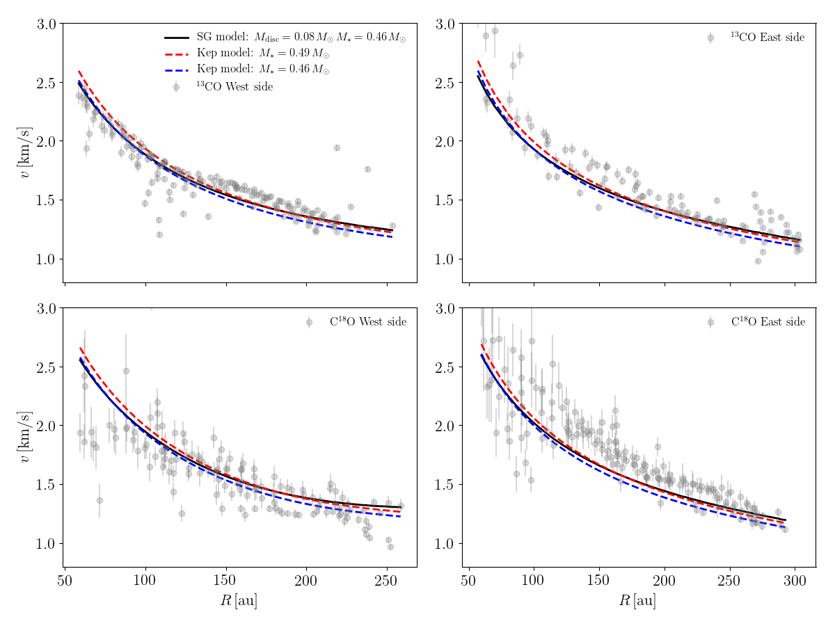
Figure 1: Rotation curve for the ¹³CO and C¹⁸O isotopologues for different models. The fitting procedure has been done simultaneously for the East (right column) and West (left column) side velocity data (plotted as grey markers), and for the two CO-isotopologues (top: ¹³CO; bottom: C¹⁸O). The black solid line corresponds to the self-gravitating fit, the red dashed line to the Keplerian fit and the blue dashed one to the Keplerian curve obtained with the star mass from the SG fit.

3.1 Combined fit

In Fig. 1 we show the results obtained with the Keplerian (see Eq. 4, red and blue dashed lines) and self-gravitating (see Eqs. 1 and 2, black solid lines) models, when simultaneously fitting all the data points (but considering the height profiles separately) for both CO isotopologues and for both sides of the disk, shown in separate panels for clarity, with the East and West side of the disk on the right and left columns, respectively, and the two CO-isotopologues (top: ¹³CO; bottom: C¹⁸O). The red line corresponds to the Keplerian best fit model, the blue line shows the rotation curve for a Keplerian disk where the star mass has been fixed to the one found with the self-gravitating best fit. The values obtained for the fit parameters are reported in the third column of Table 1. The East data points, especially for the C¹⁸O, tend to lie above the best fit curves, since in this combined fit the model naturally tends to reproduce the lower uncertainty ¹³CO data. If we first look at the power-law model, once we leave the freedom of a general power-law index, the best-fit value of the exponent $p_{2}$ is smaller than $0.5$ ($p_{2}=0.43\pm 0.03$), by more than $2\sigma$. This already suggests that the data are better reproduced by a self-gravitating model. In such a model, the disk mass obtained from the combined fit is $M_{\rm disk}=0.08\pm 0.04\,M_{\odot}$ with a star mass $M_{\star}=0.46\pm 0.03\,M_{\odot}$. Note that we obtain a non-zero measurement of the disk mass too within $\sim 2\sigma$ uncertainties. Instead, in the Keplerian case, the star mass is $M_{\star}=0.49\pm 0.01\,M_{\odot}$. For both models, the stellar mass is in agreement with previous estimates (Paneque-Carreno et al., 2021).

Table 1: Parameter obtained with a Keplerian, self-gravitating and power-law model for each CO-isotopologues (first two columns) and for a combined fit (both sides and both CO-isotopologues, third column). We also show the reduced $\chi^{2}$ difference between the Keplerian and self-gravitating fit, as $\lambda=\Delta(\chi^{2}_{\rm red})$.

	${}^{13}\mathrm{CO}$	$\mathrm{C}^{18}\mathrm{O}$	Combined fit
Keplerian fit
$M_{\star}\,[M_{\odot}]$	0.50${}^{+0.01}_{-0.01}$	0.46${}^{+0.03}_{-0.03}$	0.49${}^{+0.01}_{-0.01}$
Self-gravitating fit
$M_{\star}\,[M_{\odot}]$	$0.45^{+0.03}_{-0.03}$	$0.43^{+0.05}_{-0.07}$	$0.46^{+0.03}_{-0.03}$
$M_{\rm disk}\,[M_{\odot}]$	$0.1^{+0.05}_{-0.04}$	$0.08^{+0.08}_{-0.05}$	$0.08^{+0.04}_{-0.04}$
$\lambda=\Delta$($\chi^{2}_{\rm red}$)	2.16	-0.19	1.38
Power-law fit
$p_{1}$	$13.46^{+2.39}_{-2.07}$	$25.31^{+14.67}_{-9.39}$	$13.95^{+2.39}_{-2.06}$
$p_{2}$	$0.43^{+0.03}_{-0.03}$	$0.54^{+0.09}_{-0.1}$	$0.43^{+0.03}_{-0.03}$

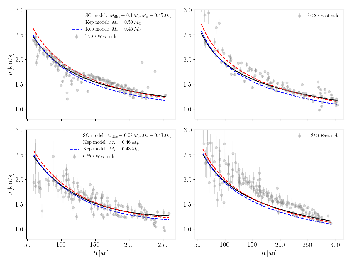
Figure 2: Rotation curve for the ¹³CO and C¹⁸O isotopologues for different models. The fitting procedure has been done simultaneously for the East (right column) and West (left column) side velocity data (plotted as grey markers). The black solid line corresponds to the self-gravitating fit, the red dashed line to the Keplerian fit and the blue dashed one to the Keplerian curve obtained with the star mass from the SG fit.

3.2 Individual isotopologues fit

We also performed a fit separately for the two CO isotopologues. The result is shown in Fig. 2, where the upper and lower panels correspond to the West (left panel) and East (right panel) side of the ¹³CO and C¹⁸O isotopologue, respectively. The parameters obtained from the best-fit models are shown in the first two columns of Table 1. Also in this case, we start by looking at the power-law model. For the ¹³CO data, the best-fit value of the exponent $p_{2}$ is again smaller than $0.5$ ($p_{2}=0.43\pm 0.03$), meaning that the self-gravitating model should be preferred to reproduce the data. In contrast, for the C¹⁸O the best-fit power-law index is $p_{2}=0.54^{+0.09}_{-0.1}$, where the value of 0.5 is inside the uncertainties, meaning that a purely Keplerian model is consistent with the ¹⁸CO data, given the larger uncertainty in the velocity points in this case. We also note that the obtained value $>0.5$ could suggest the presence of a warp or chaotic accretion from the cloud. By considering the results for the ¹³CO, best fitted by a self-gravitating model, the disk mass is $M_{\rm disk}=0.1^{+0.05}_{-0.04}\,M_{\odot}$, with a stellar mass of $M_{\star}=0.45\pm 0.03\,M_{\odot}$.

4 Discussion

Having performed fits for the self-gravitating and the Keplerian model, we now compare which one is a better fit to the data. To do so, we compute the reduced $\chi$-square ($\chi^{2}_{\rm red}$) for each model and each CO-isotopologue. We then compute the likelihood ratio $\lambda$, defined as the difference between the Keplerian and self-gravitating minimum reduced $\chi$-square:

$$\lambda=(\chi^{2}_{\rm red})_{\rm min,Kep}-(\chi^{2}_{\rm red})_{\rm min,SG}\,.$$ (7)

For Gaussian, independent measurements, this function is distributed like a $\chi^{2}$ with $n$ degrees of freedom, where $n$ is the number of new parameters in the more general case ($n=1$), with the hypothesis that the less general model is correct (i.e. the Keplerian model). The computed values are presented in Table 1. We obtain $\lambda\simeq 2.16$ for the ¹³CO fit, and $1.38$ for the combined fit, which means that the Keplerian model is rejected with respect to the self-gravitating one. If we consider only the $\mathrm{C}^{18}\mathrm{O}$ data, instead, the likelihood ratio tends to slightly prefer a simple Keplerian model (see Table 1). This means that in this case the two models are indistinguishable, possibly because the errors are larger with respect to the ${}^{13}\mathrm{CO}$ case.

In summary, the best fitting model for the combined set of data, including both available CO isotopologues is a non-Keplerian one, with a disk mass $M_{\rm disk}=0.08\pm 0.04\,M_{\odot}$, and a star mass $M_{\star}=0.46\pm 0.03\,M_{\odot}$. Considering only the ¹³CO data (that are of better quality with respect to the C¹⁸O ones), we obtain a disk mass of $M_{\rm disk}=0.1^{+0.05}_{-0.04}\,M_{\odot}$ and a star mass $M_{\star}=0.45\pm 0.03\,M_{\odot}$. In both cases, we obtain a non-zero disk mass within $2\sigma$. Instead, the C¹⁸O alone might be compatible with a purely Keplerian rotation curve, even though the self-gravitating fit returns a non-zero disk mass to within 1$\sigma$ uncertainty, $M_{\rm disk}=0.08^{+0.08}_{-0.05}\,M_{\odot}$ and a star mass of $0.43^{+0.05}_{-0.07}\,M_{\odot}$.

Thus, assuming a total disk mass equal to $0.08-0.1$ $M_{\odot}$ (and a star mass of $0.46-0.45$ $M_{\odot}$) as obtained from the fits above, we get a disk-to-star mass ratio of $\sim 0.17-0.22$. Gravitational instabilities arise when the disk-to-star mass ratio becomes of the order of the disk aspect ratio $H/R$, which is typically of the order of $\approx 0.1$ for protostellar disks. The disk mass we derive from the rotation curve is thus in the correct range to produce gravitational instabilities and thus the spiral structure observed. In particular, the observed two-armed grand-design structure is strongly suggestive of an internal origin due to gravitational instabilities. We note that from the relation between the disk-to-star mass ratio and the number of spiral arms $M_{\rm disk}/M_{\star}\propto 1/m$ (Lodato & Rice, 2004; Cossins et al., 2009; Dong et al., 2015) the obtained disk mass would point to high $m$ modes, while just two spiral arms are observed through ALMA. However, Dipierro et al. (2014) have demonstrated that, even if the density structure has an intrinsic $m>2$ spiral, smaller-scale arms can be washed out by the limited resolution of the instrument, leaving only the lowest $m$ modes in ALMA dust continuum observations. The disk mass obtained in this work is consistent with those used in the hydrodynamical simulations that reproduce the observed spirals, as performed by Paneque-Carreno et al. (2021), where they employ a disk-to-star mass ratio in the range of q = 0.1-0.3, and in the simulations of Cadman et al. (2020), with a slightly larger q = 0.27 value.

Having obtained a dynamical estimate of the total disk mass, and assuming a dust disk mass of $10^{-3}\,M_{\odot}$ (Paneque-Carreno et al., 2021; Pérez et al., 2016), we can put interesting constraints on the gas-to-dust, that turns out to be of the order of $\approx 80-100$ (for the combined fit and the ¹³CO isotopologue), which in the first case corresponds to a factor $\sim 1.2$ smaller than the usually assumed value of 100. Note that the so obtained gas-to-dust ratio estimate extremely depends on the dust mass derivation and thus it should be considered with care. For this derivation we assumed a dust mass of $10^{-3}\,M_{\odot}$, but Paneque-Carreno et al. (2021) showed that the disk being optically thick with a low spectral index, scattering could be important leading to a dust mass estimate up to 2 times larger than previously considered.

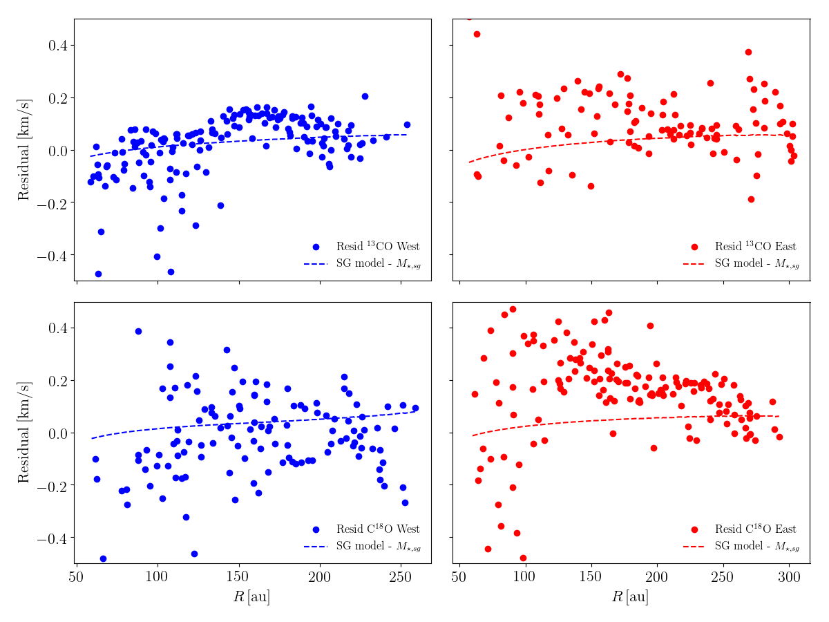
Figure 3: Residuals obtained for the combined fit. The top panels show residual for the ¹³CO (blue points and dashed line), while the bottom ones for the C¹⁸O (red points and dashed line). The left panels correspond to the West side, while the right one to the East side. Points represent the difference between the velocity data and a Keplerian model where the star mass $M_{\star,{\rm sg}}$ has been obtained through the self-gravitating model. The dashed line is the difference between the self-gravitating model and the above mentioned stellar contribution, $M_{\star,{\rm sg}}$.

As a further analysis of the results obtained in the combined fit, we show in Fig. 3 the residuals for both disk sides (left: West; right: East) and the CO-isotopologues (blue: ¹³CO; red: C¹⁸O). In particular, the points are the difference between the velocity data and a Keplerian model where the star mass $M_{\star,{\rm sg}}$ has been obtained through the self-gravitating model. The dashed line is the difference between the self-gravitating model and the Keplerian velocity with the stellar mass $M_{\star,{\rm sg}}$. From these results it appears that especially the residuals for the West side in the ¹³CO do require a significant disk contribution to the gravitational potential. Indeed, the data residuals present an increasing trend, following the disk contribution model, in particular for the West side. Instead, for the C¹⁸O there is still some large scatter in both directions. This aspect is particularly interesting, indeed, Paneque-Carreno et al. (2021) find that there is an important asymmetry between the East and West side data (see their Discussion section). The main characteristic of this asymmetry is that the West side is more compact and brighter than the East side, which is more extended and cloud-contaminated. The rotation curve on the East side then should be considered with care, since the disk can be contaminated by chaotic accretion from the cloud. This infall of material could in principle change the centrifugal balance, increasing the complexity of the system. For this reason, we decided to repeat the fit procedure for the West side only. The obtained results are described in Appendix C. We obtain an even stronger indication in favor of a self-gravitating fit, with the Keplerian fit rejected with 80% confidence for the combined fit and with 97% confidence considering the ¹³CO data only. The resulting disk mass in this case is $M_{\rm disk}=0.16\pm 0.06\,M_{\odot}$ with a stellar mass $M_{\star}=0.41\pm 0.04\,M_{\odot}$, and thus in a disk-to-star mass ratio of $\sim 0.40$.

Finally, it has to be noted that small scale gas turbulence could contribute to deviations from keplerian motion, but this generally amounts to no more than $\ 0.1c_{\rm s}\sim 20$ m/s (Flaherty et al., 2020), being thus smaller than the observed deviation (the disk contribution is $\sim 50-100$ m/s, see Fig. 3).

5 Conclusions

In this paper we have looked for deviations from Keplerian rotation in the disk orbiting around the Elias 2-27 system, providing for the first time a dynamical measurement of the total mass of a planet forming disk, by fitting its rotation curve as derived from CO emission with a model including both the stellar and the disk contribution to the gravitational field. We performed three different fit procedures, that is, a combined fit considering both disk sides and both CO-isotopologues, an individual fit to the data points for the separate isotopologues, and a third fit considering only the less cloud-contaminated West side of the disk; the last case is described in Appendix C. The outcome of these analysis is that the ¹³CO isotopologues data, and in particular the West side of the disk, are better reproduced by a self-gravitating disk model rather than a pure Keplerian one. The same is true also considering both isotopologues, although with smaller confidence, with a resulting disk mass of $M_{\rm disk}=0.08\pm 0.04\,M_{\odot}$ and a stellar mass $M_{\star}=0.46\pm 0.03\,M_{\odot}$ (where the stellar mass is compatible with previous estimates). We point out that we obtain a non-zero measure of the disk mass within 2$\sigma$ uncertainty, both in the combined fit and in the fit for the ¹³CO isotopologue alone. Assuming these values for the disk and star mass, and assuming a dust disk mass of $10^{-3}\,M_{\odot}$ (Paneque-Carreno et al., 2021; Pérez et al., 2016), we obtain a disk-to-star mass ratio of $\simeq$ 0.17 and a gas-to-dust ratio of $\simeq 80$. These results highlight the fact that Elias 2-27 should be considered as a self-gravitating disk, reinforcing the internal gravitational instability interpretation for the observed spiral structures. This result is more evident when fitting for the ¹³CO data on the West side of the disk, that are less contaminated by the cloud contamination and possible infall (Paneque-Carreno et al., 2021) for which we obtain a disk-to-star mass ratio of $\sim 0.40$, with a disk mass of $0.16\,M_{\odot}$ and a star mass of $0.41\,M_{\odot}$. We point out that the lower confidence level obtained in the combined isotopologues fit is due to the relatively lower quality of the C¹⁸O data, which can be improved in future observations.

Finally, we remark that this method to estimate the disk mass can be applied to other protoplanetary disks (such as, for example, IM Lup and WaOph 6 from the DSHARP sample, Huang et al. 2018a, and RU Lup, Huang et al. 2020, that also show a prominent spiral structure), aiming to give better constraints (independent of CO or dust to H₂ conversion) on the disk mass. Such measurement can also be used to calibrate the conversion factors between dust and total mass, at least for these systems.

Appendix A Corner plot results for the combined fit

Fig. 4 collects the corner plots of the MCMC procedure for the Keplerian (left), self-gravitating (disk+star, centre) and power-law (right) fit of the CO isotopologues velocity data for the combined fit. The fit results correspond to those discussed in Sec. 3.1. The final masses and errors are computed from the median value, 16th and 84th percentile uncertainties derived from the posteriors.

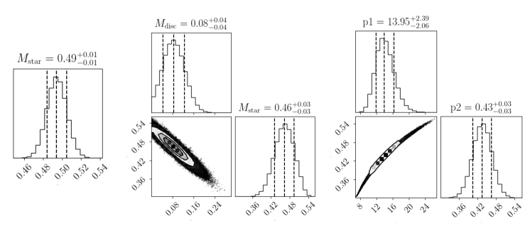
Figure 4: Probability distribution and corner plots obtained with the Keplerian (left), disk+star (centre) and power law (right) model for the total fit, where the East and West sides, and the ¹³CO and C¹⁸O data have been fitted simultaneously.

Appendix B Corner plot results for the individual isotopologues fit

Fig. 5 collects the corner plots of the MCMC procedure for the Keplerian (left panels), self-gravitating (disk+star, central panels) and power-law (right panels) fit of the CO isotopologues velocity data (upper panels: ¹³CO; lower panels: C¹⁸O), fitted separately. The fit results correspond to those discussed in Sec. 3.2. The final masses and errors are computed from the median value, 16th and 84th percentile uncertainties derived from the posteriors.

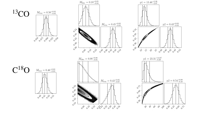
Figure 5: Probability distribution and corner plots for different models (from left to right: Keplerian, disk+star,power law model) for the ¹³CO (upper panels) and C¹⁸O (lower panels) isotopologues.

Appendix C West side fit

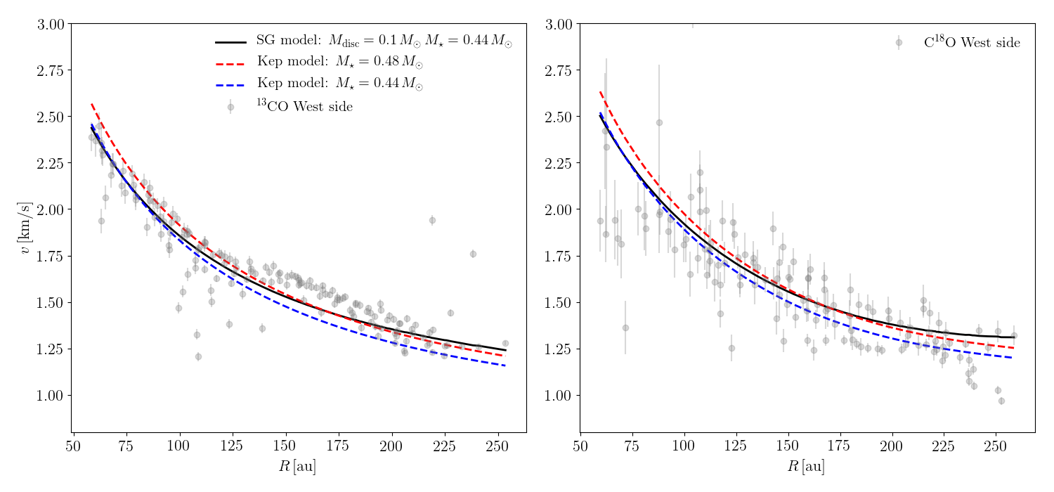
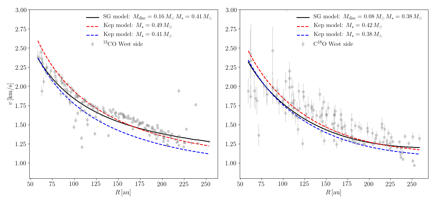
Figure 6: Top panels: rotation curve for the ¹³CO (left) and C¹⁸O (right) isotopologues for different models. In this case the fitting procedure has been performed considering only the West side of the disk. The black solid line corresponds to the self-gravitating fit and the red and blue dashed lines to the Keplerian fit and to the Keplerian curve obtained with the star mass from the SG fit, respectively. Grey markers represent the velocity data. Bottom panels: same as above, but with a fit performed separately for the two CO-isotopologues.

In Fig. 6 we show results where the fit has been done only for the West side, which is less contaminated by the infalling cloud. As in Sec. 3, the models we choose are a self-gravitating model (black solid lines), a Keplerian one (red dashed line), and a simple power-law model (see Eq. 6). As before, the blue dashed line represent the Keplerian rotation curve with the star mass fixed to the value obtained with the self-gravitating fit. The top panels collect results obtained for the combined fit, while the bottom panels show results when fitting separately the two CO-isotopologues. In Table 2 we report the obtained parameter values for each model, each CO-isotopologues (first two columns), and for the combined fit (fitting simultaneously the CO-isotopologues data, third column).

Table 2: System parameters obtained with a Keplerian, self-gravitating and power-law models for the West side disk fit. The first two columns collect results for a fit when considering separately the two CO-isotopologues, the third one when considering them simultaneously. We also show the reduced $\chi^{2}$ difference between the Keplerian and self-gravitating fit, as $\lambda=\Delta$($\chi^{2}_{\rm red}$).

	${}^{13}\mathrm{CO}$	$\mathrm{C}^{18}\mathrm{O}$	Combined fit
Keplerian fit
$M_{\star}\,[M_{\odot}]$	0.49${}^{0.01}_{-0.01}$	0.42${}^{0.03}_{-0.03}$	0.48${}^{+0.01}_{-0.01}$
Self-gravitating fit
$M_{\star}\,[M_{\odot}]$	$0.41^{+0.04}_{-0.04}$	$0.38^{+0.06}_{-0.07}$	$0.44^{+0.04}_{-0.04}$
$M_{\rm disk}\,[M_{\odot}]$	$0.16^{+0.06}_{-0.06}$	$0.08^{+0.08}_{-0.06}$	$0.1^{+0.06}_{-0.05}$
$\lambda=\Delta$($\chi^{2}_{\rm red}$)	4.57	-0.51	1.58
Power-law fit
$p_{1}$	$12.66^{+3.47}_{-2.75}$	$27.49^{+23.67}_{-13.33}$	$14.07^{+3.53}_{-2.85}$
$p_{2}$	$0.42^{+0.05}_{-0.05}$	$0.58^{+0.12}_{-0.13}$	$0.44^{+0.04}_{-0.04}$

The resulting disk mass in the combined fit is $M_{\rm disk}=0.1^{+0.06}_{-0.05}\,M_{\odot}$, with a stellar mass of $M_{\star}=0.44\pm 0.04\,M_{\odot}$. The obtained likelihood ratio $\lambda=\Delta\chi^{2}_{\rm red}\sim 1.6$ implies a rejection of the Keplerian model.This values would provide a disk-to-star mass ratio of 0.22, meaning that the disk mass is in the right range to give rise to gravitational instabilities. Also when considering the CO-isotopologues separately, this behaviour is seen for the ¹³CO. In this case, the expected disk mass is $M_{\rm disk}=0.16\pm 0.06\,M_{\odot}$, the stellar mass $M_{\star}=0.41\pm 0.04\,M_{\odot}$ and $\lambda=\Delta\chi^{2}_{\rm red}\sim 4.6$, implying also in this case a rejection of the Keplerian model. These values correspond to a disk-to-star mass ratio of 0.39.

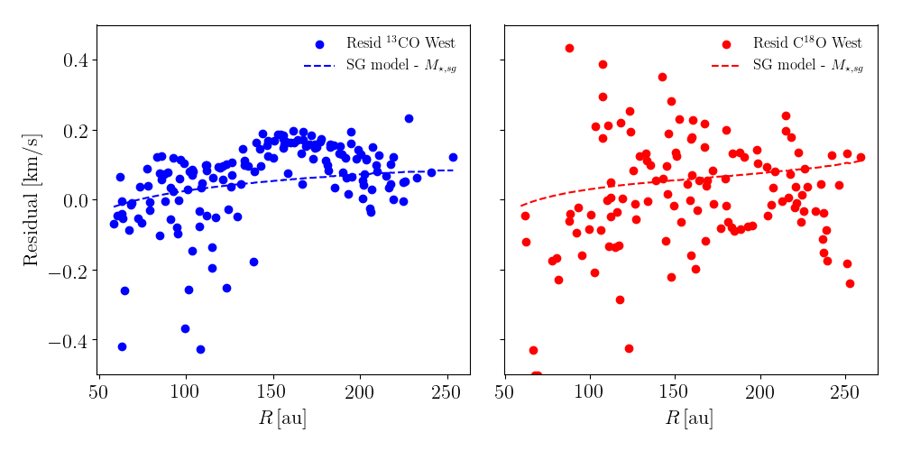
Figure 7: Residuals obtained for the West side fit, when considering simultaneously the two CO-isotopologues. The left panel shows residual for the ¹³CO (blue markers and dashed line), while the right one for the C¹⁸O (red markers and dashed line). Markers represent the difference between the velocity data and a Keplerian model where the star mass $M_{\star,{\rm sg}}$ has been obtained through the self-gravitating model. The dashed line is the difference between the self-gravitating model and the above mentioned star contribution, $M_{\star,{\rm sg}}$.

For the combined (both CO- isotopologues) West fit, we collect in Fig. 7 the residuals. The difference between the self-gravitating model and the star contribution to the gravitational potential (as obtained with the self-gravitating model) shows that the disk contribution fits well the data residual (data - Keplerian mass), especially for the ¹³CO isotopologue.

C.1 Corner plot results

Fig. 8 collects the probability distribution and corner plots obtained with the Keplerian (left), self-gravitating (disk+star, centre) and power-law (right) fit of the CO isotopologues velocity data, when fitting the West side, simultaneously for the ¹³CO and C¹⁸O isotopologues. Fig. 9 shows the same results but for a fit where the two CO-isotopologues (top: ¹³CO; bottom: C¹⁸O) have been fitted separately.

The fit results correspond to those discussed in Sec. C. The final masses and errors are computed from the median value, 16th and 84th percentile uncertainties derived from the posteriors.

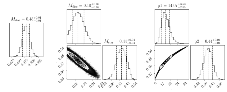
Figure 8: Probability distribution and corner plots obtained with the Keplerian (left), disk+star (centre) and power law (right) model for the West side, where the ¹³CO and C¹⁸O data have been fitted simultaneously.

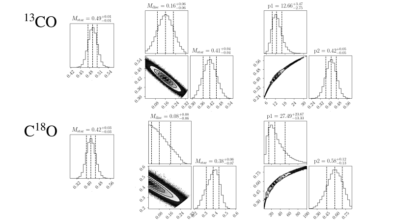
Figure 9: Probability distribution and corner plots obtained with the Keplerian (left), disk+star (centre) and power law (right) model for the West side, where the ¹³CO (upper panels) and C¹⁸O (lower panels) data have been fitted separately.

References

- Andrews et al. (2018) Andrews, S. M., Terrell, M., Tripathi, A., et al. 2018, ArXiv e-prints, arXiv:1808.10510
- Andrews et al. (2009) Andrews, S. M., Wilner, D. J., Hughes, A. M., Qi, C., & Dullemond, C. P. 2009, ApJ, 700, 1502
- Ansdell et al. (2016) Ansdell, M., Williams, J. P., van der Marel, N., et al. 2016, ApJ, 828, 46
- Bae & Zhu (2018) Bae, J., & Zhu, Z. 2018, ApJ, 859, 119
- Barbieri et al. (2005) Barbieri, C. V., Fraternali, F., Oosterloo, T., et al. 2005, A&A, 439, 947
- Bergin & Williams (2018) Bergin, E. A., & Williams, J. P. 2018, arXiv e-prints, arXiv:1807.09631
- Bergin et al. (2013) Bergin, E. A., Cleeves, L. I., Gorti, U., et al. 2013, Nature, 493, 644
- Bertin & Lodato (1999) Bertin, G., & Lodato, G. 1999, A&A, 350, 694
- Bosman et al. (2018) Bosman, A. D., Walsh, C., & van Dishoeck, E. F. 2018, A&A, 618, A182
- Cadman et al. (2020) Cadman, J., Hall, C., Rice, K., Harries, T. J., & Klaassen, P. D. 2020, MNRAS, 498, 4256
- Calcino et al. (2020) Calcino, J., Christiaens, V., Price, D. J., et al. 2020, MNRAS, 498, 639
- Cleeves et al. (2018) Cleeves, L. I., Öberg, K. I., Wilner, D. J., et al. 2018, ApJ, 865, 155
- Cossins et al. (2009) Cossins, P., Lodato, G., & Clarke, C. J. 2009, MNRAS, 393, 1157
- Dipierro et al. (2014) Dipierro, G., Lodato, G., Testi, L., & de Gregorio Monsalvo, I. 2014, MNRAS, 444, 1919
- Dong et al. (2015) Dong, R., Hall, C., Rice, K., & Chiang, E. 2015, ApJ, 812, L32
- Draine (2003) Draine, B. T. 2003, ARA&A, 41, 241
- Favre et al. (2013) Favre, C., Cleeves, L. I., Bergin, E. A., Qi, C., & Blake, G. A. 2013, ApJ, 776, L38
- Flaherty et al. (2020) Flaherty, K., Hughes, A. M., Simon, J. B., et al. 2020, ApJ, 895, 109
- Foreman-Mackey (2016) Foreman-Mackey, D. 2016, The Journal of Open Source Software, 1, 24. https://doi.org/10.21105/joss.00024
- Foreman-Mackey et al. (2013) Foreman-Mackey, D., Hogg, D. W., Lang, D., & Goodman, J. 2013, PASP, 125, 306
- Forgan et al. (2018) Forgan, D. H., Ilee, J. D., & Meru, F. 2018, ApJ, 860, L5
- Gaia Collaboration et al. (2018) Gaia Collaboration, Brown, A. G. A., Vallenari, A., et al. 2018, A&A, 616, A1
- Gradshteyn & Ryzhik (1980) Gradshteyn, I. S., & Ryzhik, I. M. 1980, Table of integrals, series and products
- Hall et al. (2018) Hall, C., Rice, K., Dipierro, G., et al. 2018, MNRAS, 477, 1004
- Hall et al. (2020) Hall, C., Dong, R., Teague, R., et al. 2020, ApJ, 904, 148
- Huang et al. (2018a) Huang, J., Andrews, S. M., Pérez, L. M., et al. 2018a, ApJ, 869, L43
- Huang et al. (2018b) Huang, J., Andrews, S. M., Dullemond, C. P., et al. 2018b, ApJ, 869, L42
- Huang et al. (2020) Huang, J., Andrews, S. M., Öberg, K. I., et al. 2020, ApJ, 898, 140
- Hunter (2007) Hunter, J. D. 2007, Computing in Science and Engineering, 9, 90
- Ilee et al. (2017) Ilee, J. D., Forgan, D. H., Evans, M. G., et al. 2017, MNRAS, 472, 189
- Kratter & Lodato (2016) Kratter, K., & Lodato, G. 2016, ARA&A, 54, 271
- Lodato & Bertin (2003) Lodato, G., & Bertin, G. 2003, A&A, 398, 517
- Lodato & Rice (2004) Lodato, G., & Rice, W. K. M. 2004, MNRAS, 351, 630
- Long et al. (2017) Long, F., Herczeg, G. J., Pascucci, I., et al. 2017, ApJ, 844, 99
- Luhman & Rieke (1999) Luhman, K. L., & Rieke, G. H. 1999, ApJ, 525, 440
- Macias et al. (2021) Macias, E., Guerra-Alvarado, O., Carrasco-Gonzalez, C., et al. 2021, arXiv e-prints, arXiv:2102.04648
- Meru et al. (2017) Meru, F., Juhász, A., Ilee, J. D., et al. 2017, ApJ, 839, L24
- Miotello et al. (2016) Miotello, A., van Dishoeck, E. F., Kama, M., & Bruderer, S. 2016, A&A, 594, A85
- Miotello et al. (2017) Miotello, A., van Dishoeck, E. F., Williams, J. P., et al. 2017, A&A, 599, A113
- Paneque-Carreno et al. (2021) Paneque-Carreno, T., Perez, L. M., Benisty, M., et al. 2021, arXiv e-prints, arXiv:2103.14048
- Pascucci et al. (2016) Pascucci, I., Testi, L., Herczeg, G. J., et al. 2016, ApJ, 831, 125
- Pérez et al. (2016) Pérez, L. M., Carpenter, J. M., Andrews, S. M., et al. 2016, Science, 353, 1519
- Pinte et al. (2018) Pinte, C., Ménard, F., Duchêne, G., et al. 2018, A&A, 609, A47
- Pinte et al. (2020) Pinte, C., Price, D. J., Ménard, F., et al. 2020, ApJ, 890, L9
- Pringle (1981) Pringle, J. E. 1981, ARA&A, 19, 137
- Quénard et al. (2018) Quénard, D., Jiménez-Serra, I., Viti, S., Holdship, J., & Coutens, A. 2018, MNRAS, 474, 2796
- Rice et al. (2004) Rice, W. K. M., Lodato, G., Pringle, J. E., Armitage, P. J., & Bonnell, I. A. 2004, MNRAS, 355, 543
- Rice et al. (2006) —. 2006, MNRAS, 372, L9
- Trapman et al. (2017) Trapman, L., Miotello, A., Kama, M., van Dishoeck, E. F., & Bruderer, S. 2017, A&A, 605, A69
- van der Marel et al. (2020) van der Marel, N., Birnstiel, T., Garufi, A., et al. 2020, arXiv e-prints, arXiv:2010.10568
- Veronesi et al. (2019) Veronesi, B., Lodato, G., Dipierro, G., et al. 2019, MNRAS, 489, 3758
- Williams & Best (2014) Williams, J. P., & Best, W. M. J. 2014, ApJ, 788, 59
- Zhang et al. (2018) Zhang, S., Zhu, Z., Huang, J., et al. 2018, ApJ, 869, L47