Kinematics of MgII Absorbers from the Redshift-space Distortion Around Massive Quiescent Galaxies

Abstract

The kinematics of MgII absorbers is the key to understanding the origin of cool, metal-enriched gas clouds in the circumgalactic medium of massive quiescent galaxies. Exploiting the fact that the cloud line-of-sight velocity distribution is the only unknown for predicting the redshift–space distortion (RSD) of MgII absorbers from their 3D real–space distribution around galaxies, we develop a novel method to infer the cool cloud kinematics from the redshift–space galaxy–cloud cross–correlation $\xi^{s}$. We measure $\xi^{s}$ for ${\sim}10^{4}$ MgII absorbers around ${\sim}8{\times}10^{5}$ CMASS galaxies at $0.4{<}z{<}0.8$. We discover that $\xi^{s}$ does not exhibit a strong Fingers-of-God effect, but is heavily truncated at velocity ${\sim}300\,\mathrm{km}\,s^{-1}$. We reconstruct both the redshift and real–space cloud number density distributions inside haloes, $\xi^{s}_{1h}$ and $\xi_{1h}$, respectively. Thus, for any model of cloud kinematics, we can predict $\xi^{s}_{1h}$ from the reconstructed $\xi_{1h}$, and self–consistently compare to the observed $\xi^{s}_{1h}$. We consider four types of cloud kinematics, including an isothermal model with a single velocity dispersion, a satellite infall model in which cool clouds reside in the subhaloes, a cloud accretion model in which clouds follow the cosmic gas accretion, and a tired wind model in which clouds originate from the galactic wind–driven bubbles. All the four models provide statistically good fits to the RSD data, but only the tired wind model can reproduce the observed truncation by propagating ancient wind bubbles at ${\sim}250\,\mathrm{km}\,s^{-1}$ on scales ${\sim}400\,h^{-1}\mathrm{kpc}$. Our method provides an exciting path to decoding the dynamical origin of metal absorbers from the RSD measurements with upcoming spectroscopic surveys.

1 Introduction

The circumgalactic space in dark matter haloes is permeated by multi-phase gas with temperatures ranging from $10^{2}$ to $10^{8}$ K and densities between $10^{-6}$ to $1$ cm^-3  (Tumlinson et al., 2017). One of the most intriguing puzzles of the circumgalactic medium (CGM) is the apparent abundance of cool (${\sim}10^{4}$ K), metal-enriched gas clouds (e.g., detected via the MgII absorption doublets in rest-frame UV along quasar sightlines; Bergeron & Boissé, 1991; Steidel & Sargent, 1992; Steidel et al., 1994; Churchill et al., 1999), embedded in the hot ($T{>}10^{6}\,$K) gaseous corona (Spitzer, 1956; Anderson et al., 2013) surrounding massive quiescent galaxies (Thom et al., 2012; Prochaska et al., 2013; Werk et al., 2014; Keeney et al., 2017). Particularly, it is unclear whether the cool clouds are governed by random, inflowing, or outflowing motion (Lan & Mo, 2019). In this paper, we explore the kinematics of MgII absorbers around a large sample of luminous red galaxies (LRGs) observed by the Baryon Oscillation Spectroscopic Survey (BOSS; Dawson et al., 2013) at $z{\sim}0.55$, in hopes of paving the path for a self–consistent redshift–space distortion (RSD) modelling of metal absorbers with upcoming spectroscopic surveys like the DESI (Levi et al., 2019) and PFS (Takada et al., 2014).

While the hot corona can be naturally explained by the shock-heating of inflowing gas to the virial temperature of massive dark matter haloes (Birnboim & Dekel, 2003; Kereš et al., 2005; Dekel et al., 2009), the physical origin of the cool, metal-enriched CGM gas surrounding massive quiescent galaxies remains largely elusive  (Chen, 2017, and references therein). This is mainly due to the lack of galactic winds driven by recent star formation in those systems, and winds are the dominant means of transporting enriched material into the CGM (Oppenheimer & Davé, 2006; Peeples & Shankar, 2011; Davé et al., 2011; Hummels et al., 2013; Ford et al., 2014; Ma et al., 2016; Fielding et al., 2017; Muratov et al., 2017; Fielding et al., 2020). Around star-forming galaxies, cool gas clouds are commonly seen as blue-shifted absorption and emission in galactic winds (see Heckman & Thompson, 2017; Veilleux et al., 2020, and references therein). They could be dragged into the CGM via entrainment in a fast-moving hot wind (but see Zhang et al., 2017), accelerated by radiation or cosmic ray pressure (Murray et al., 2005; Kim & Ostriker, 2018), or formed out of radiative cooling of the hot wind material (Wang, 1995; Thompson et al., 2016). Without ongoing star-forming or quasar (Cai et al., 2019) activities, it is unclear whether galactic winds remain a viable channel for producing cool CGM gas in massive quiescent galaxies.

One possibility is that the galactic winds launched during the star formation episodes prior to quenching may survive more than a few Gyrs. Recently, Lochhaas et al. (2018) developed an 1D semi-analytic model of CGM as long-lived bubbles blown by galactic winds, which then shock and sweep up ambient halo gas as they propagate outward from the host galaxy (also see Samui et al., 2008; Sarkar et al., 2015). They showed that the shocked wind can radiatively cool to $10^{4}$ K and the cooled massive shells can travel to several hundred $\mathrm{kpc}$s with $v{\sim}100{-}300\mathrm{km}\,s^{-1}$ within a span of $1{-}10$ Gyrs. Therefore, the bubble effectively “hangs” at a large distance from the galaxy for a long time, explaining the presence of wind material in the CGM surrounding quiescent galaxies. Since Lochhaas et al. (2018) mainly focused on the Milky Way-sized haloes with $M_{h}{\simeq}10^{12}M_{\odot}$ probed by COS-HALO (Tumlinson et al., 2013), it is unclear if the results also applies to the LRG-size haloes with $M_{h}{\gtrsim}10^{13}M_{\odot}$.

Apart from galactic winds, cool clouds could also appear in the CGM of massive quiescent galaxies via cosmological gas accretion (Kereš et al., 2009; Fumagalli et al., 2011; van de Voort et al., 2012), gas stripping from satellite infall (Gauthier et al., 2010; Gauthier, 2013; Lee et al., 2021), and condensation due to thermal instability in the hot medium (Mo & Miralda-Escude, 1996; Maller & Bullock, 2004; Sharma et al., 2012; McCourt et al., 2012; Voit & Donahue, 2015; Voit, 2018; Nelson et al., 2020). All three scenarios above involve the infall of cool clouds through the hot halo gas while experiencing effects of hydrodynamic drag and cloud evaporation (Armillotta et al., 2017), modulo differences in the initial cloud conditions. For example, Afruni et al. (2019) developed a semi-analytic model for cloud accretion from the intergalactic medium, finding that the accretion of clouds with cloud mass $M_{\mathrm{cl}}{\sim}10^{5}M_{\odot}$ could reproduce the velocity distribution and column densities of the cool clouds observed by COS-LRG (Chen et al., 2018; Zahedy et al., 2019). Meanwhile, those clouds will evaporate before reaching the host galaxy, therefore unlikely rejuvenating any star formation. However, there is no appreciable difference between the observed metallicity distributions of the star–forming and quiescent galaxies (Lehner et al., 2013; Berg et al., 2019). Therefore, without the enrichment from stellar outflows, it is unclear how the newly accreted cool gas becomes significantly metal-enriched while in pressure equilibrium with the hot gas.

The key to distinguishing between the wind vs. no–wind origins lies in the kinematics of the cool clouds. The most common probe of the cloud kinematics is the distribution of redshifts of MgII absorbers relative to their host galaxies $\Delta z$. In particular, $\Delta z$ is usually interpreted in the literature as the relative line-of-sight (LOS) velocity of MgII absorbers (normalized by the speed of light $c$), so that $c\Delta z\simeq{v}_{\mathrm{los}}(1+z)$. This approximation, however, ignores the fact that $\Delta z$ also depends on the comoving distance between the two systems along the LOS, $y$ , so that $c\Delta z={v}_{\mathrm{los}}(1+z)+H_{z}y$, where $H_{z}$ is the Hubble parameter at $z$. The approximation is more than adequate for comparing the LOS velocity dispersion of the MgII absorbers to that of the dark matter (see e.g., Huang et al., 2016), but for a more stringent test of cloud kinematic models we need to explicitly model the redshift-space galaxy-absorber cross–correlation functions (Lanzetta et al., 1998; Chen et al., 2005; Ryan-Weber, 2006; Wilman et al., 2007; Chen & Mulchaey, 2009; Tejos et al., 2012; Borthakur et al., 2016). In this paper, we will first reconstruct the 3D spatial distribution of cool clouds from the observed projected LRG-MgII cross-correlation function, and then infer the velocity distribution from the observed RSD of MgII absorbers around LRGs. A similar method was first developed by  Zu & Weinberg (2013) for inferring the galaxy infall kinematics around massive galaxy clusters.

This paper is organized as follows. We describe the BOSS LRG and the MgII absorber catalogues in §2. The RSD measurements are presented in §3. We present our reconstruction of the 3D distribution of MgII absorbers within the LRG haloes and extract the small-scale RSD signal of MgII absorbers in §4. We compare the theoretical predictions of RSD from different kinematic models in §5 before we summarise our results and look to the future in §6. Throughout this paper, we assume the Planck cosmology (Planck Collaboration et al., 2020). All the length and mass units in this paper are scaled as if the Hubble constant is $100\,\mathrm{km}\,s^{-1}\mathrm{Mpc}^{-1}$. In particular, all the separations are co-moving distances in units of $h^{-1}\mathrm{Mpc}$, and the halo mass is in the unit of $h^{-1}M_{\odot}$. We use $\lg x{=}\log_{10}x$ for the base-$10$ logarithm.

2 Data

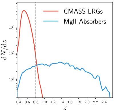
Figure 1: The redshift distributions of CMASS LRGs (red) and MgII absorbers (blue) between $z{=}0.4$ and $2.5$. The gray dashed vertical line indicates the maximum redshift ($z{=}0.8$) of our cross-correlation analysis.

2.1 Luminous Red Galaxies from BOSS CMASS

We employ the BOSS CMASS galaxy sample derived from the Data Release 12 (DR12; Alam et al., 2015) of Sloan Digital Sky Survey (SDSS; York et al., 2000). As part of the SDSS-III (Eisenstein et al., 2011), BOSS (Dawson et al., 2013) measured the spectra of 1.5 million galaxies over a sky area of ${\sim}$10,000 deg² using the BOSS spectrographs (Smee et al., 2013; Bolton et al., 2012) onboard the 2.5-m Sloan Foundation Telescope at the Apache Point Observatory (Gunn et al., 1998, 2006). The BOSS LRGs were selected from the Data Release 8 (DR8; Aihara et al., 2011) of SDSS five-band imaging (Fukugita et al., 1996) using two separate sets of colour and magnitude cuts for the LOWZ ($z{<}0.4$) and CMASS ($z{>}0.4$) samples, respectively (Reid et al., 2016). For maximal redshift overlap with the MgII absorbers, we select $823193$ CMASS galaxies with $z\in[0.4,0.8]$ as our LRG sample for cross-correlating with the MgII absorbers. We generate a random galaxy sample based on the standard CMASS random galaxy catalogue provided in the public SDSS DR12 directory, by applying the redshift distribution of the observed galaxy sample to the random catalogue (red curve in Figure 1). To minimize the shot noise from the random, we use 50 times more galaxies in the random than in the observed data set.

2.2 MgII Absorbers

We select a sample of $9088$ MgII absorbers within the CMASS footprint with $z\in[0.4,0.8]$ from the JHU-SDSS MgII absorber catalogue derived by Zhu & Ménard (2013), who applied an automatic absorption-line detection algorithm to ${\sim}140000$ quasar spectra from the SDSS DR5 (Schneider et al., 2010) and DR12 (Pâris et al., 2017). Using a novel nonnegative matrix factorization technique to estimate the quasar continua, Zhu & Ménard (2013) detected $61974$ unique MgII absorbers between $0.4<z<5.5$. The completeness and purity of the absorber catalogue are further validated with the visually inspected Pittsburgh MgII catalogue (Quider et al., 2011) derived from SDSS DR4. For cross-correlating with the CMASS galaxies, we limit our sample to absorbers within the CMASS footprint and with $z\in[0.4,0.8]$, yielding $9088$ MgII absorbers in the final sample. We do not select absorbers by their equivalent width (EW), but will apply the values of equivalent width as individual weights when computing the correlation functions.

The MgII absorbers were detected along the sightlines of SDSS quasars, which generally were given a higher target priority by the SDSS tiling algorithm (Blanton et al., 2003) than galaxies. Therefore, in order to build a truly random catalogue of MgII absorbers, we need to mimic the spectroscopic survey strategy of SDSS, so that the conditional fibre assignment probability of quasars at any angular separation away from a foreground galaxy is exactly preserved in the random absorber catalogue. Since this conditional probability is analytically intractable, we make use of the parent quasar catalogue that Zhu & Ménard (2013) searched for MgII absorbers, and randomly assign redshifts of the detected MgII absorbers to the angular coordinates of the observed quasars. To remove any potential systematics associated with the difference between DR7 and DR12 quasars, we assign the redshifts of DR7 absorbers to the coordinates of DR7 quasars, and vice versa for DR12. This random generation scheme also eliminates any systematic bias due to the intrinsic clustering of quasar sightlines (Gauthier et al., 2010). Finally, we shuffle the redshifts of the detected MgII absorbers ten times to build a random absorber catalogue ten times the size of the data catalogue.

Figure 1 shows the redshift distributions of CMASS LRGs (red) and MgII absorbers (blue) between $z{=}0.4$ and $2.5$. The dashed vertical line indicates the maximum redshift ($z{=}0.8$) of our analysis, beyond which the number density of CMASS LRGs declines rapidly. We note that the number density of MgII absorbers stays relative flat within the vast redshift range between $z{=}0.8$ and $1.8$, leaving huge statistical potential to future surveys that will target a high number density of LRGs and emission lines galaxies within the same redshift range.

3 Galaxy-cloud Cross-correlation Function in Redshift-space $\mathbf{\xi_{\mathrm{\tt{LRG-MgII}}}^{s}}$

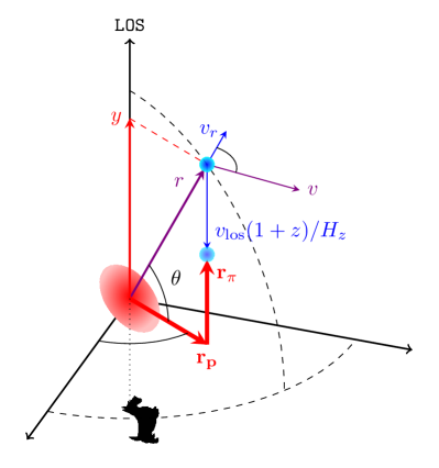
Figure 2: Schematic diagram of the redshift-space distortion of a MgII absorber (dark-shaded blue circle) in the halo of an LRG (red ellipse) at redshift $z$. The observer is at the bottom of the diagram, making the line-of-sight direction vertically upward. The LOS velocity ${v}_{\mathrm{los}}$ shifts the cloud from its real-space LOS distance $y$ by ${v}_{\mathrm{los}}(1+z)/H_{z}$ to $r_{\pi}$ (light-shaded blue circle), where $H_{z}$ is the Hubble parameter at $z$.

Before presenting the redshift-space cross-correlation function between CMASS LRGs and MgII absorbers $\xi_{\mathrm{\tt{LRG-MgII}}}^{s}$, we introduce the notations relevant to describing cloud kinematics in the galacto-centric coordinates in Figure 2. The red ellipse indicates the position of the LRG at redshift $z$, with the LOS direction pointing vertically upward. The dark-shaded blue circle indicates the real-space position of a cool cloud, with 3D distance $r$ away from the LRG, which can be further decomposed into a projected separation $r_{p}$ and an LOS distance $y$. However, unlike $r_{p}$, $y$ is not directly accessible through observations, because the relative velocity of the cloud $v$ has an LOS component ${v}_{\mathrm{los}}$ that displaces the observed position of the cloud (light-shaded blue circle) to $r_{\pi}$ along the LOS by ${v}_{\mathrm{los}}(1+z)/H_{z}$. Obviously, to recover the kinematics of the cool clouds (${v}_{\mathrm{los}}$), we need to infer both the real and redshift–space distributions of the cool clouds ($y$ and $r_{\pi}$).

3.1 Correlation Function Measurements

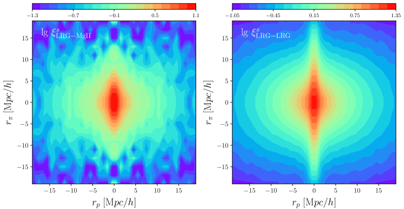
Figure 3: Left: Redshift-space cross-correlation function between LRGs and MgII absorbers; Right: Redshift-space auto-correlation function of LRGs. The logarithmic values of the correlation functions are indicated by the colour bars on top. The $0.25$ dex shift between the two colour bars accounts for the difference in the large-scale bias between MgII absorbers and LRGs. The small-scale Fingers-of-God effect is pronounced in the right panel, but weak in the left panel.

We measure $\xi_{\mathrm{\tt{LRG-MgII}}}^{s}$ using the Landy & Szalay (1993) estimator,

$$\xi_{\mathrm{\tt{LRG-MgII}}}^{s}(r_{p},r_{\pi})=\frac{D_{g}D_{c}-D_{g}R_{c}-R_{g}D_{c}+R_{g}R_{c}}{R_{g}R_{c}},$$ (1)

where $D_{g}D_{c}$ and $R_{g}R_{c}$ are the number counts of data galaxy–data cloud pairs and random galaxy–random cloud pairs at 2D separation $(r_{p},r_{\pi})$, respectively. By the same token, $D_{g}R_{c}$ and $R_{g}D_{c}$ indicate the corresponding number counts of data galaxy-random cloud pairs and random galaxy-data cloud pairs. For computing pair counts associated with the data clouds, we weigh each pair by the EW of the MgII absorber (the sum of the doublet EWs). We also repeat our analysis in this paper using measurements without the EW weights, and discover that the impact of weights on our conclusions is negligible.

To compare the RSD of MgII absorbers with that of galaxies, we also measure the redshift–space galaxy auto–correlation functions via

$$\xi_{\mathrm{\tt{LRG-LRG}}}^{s}(r_{p},r_{\pi})=\frac{D_{g}D_{g}-2D_{g}R_{g}+R_{g}R_{g}}{R_{g}R_{g}}.$$ (2)

The difference between $\xi_{\mathrm{\tt{LRG-MgII}}}^{s}$ and $\xi_{\mathrm{\tt{LRG-LRG}}}^{s}$ on large scales should be a constant shift in amplitude by a factor of $b_{g}/b_{c}$, where $b_{g}$ and $b_{c}$ are the large-scale clustering biases of the LRGs and MgII absorbers, respectively. On small scales, however, any difference between the two would be primarily induced by the deviation of cloud kinematics from that of the luminous red satellites within the haloes.

For reconstructing the 3D number density profile of the clouds, we measure the projected galaxy–cloud cross–correlations $w_{p}$ from the same data and random galaxy samples using an integration length of $r_{\pi}^{\mathrm{max}}=40\,h^{-1}\mathrm{Mpc}$, so that

$$w_{p}(r_{p})=\int_{-r_{\pi}^{\mathrm{max}}}^{+r_{\pi}^{\mathrm{max}}}\!\xi_{\mathrm{\tt{LRG-MgII}}}^{s}(r_{p},r_{\pi})\,\mathrm{d}r_{\pi}.$$ (3)

Finally, we estimate the measurement uncertainties on $\xi_{\mathrm{\tt{LRG-MgII}}}^{s}$ and $w_{p}$ using the standard Jackknife re–sampling method by dividing the CMASS sky coverage into $200$ approximately equal-area regions (Norberg et al., 2009).

3.2 Comparison between $\mathbf{\xi_{\mathrm{\tt{LRG-MgII}}}^{s}}$ and $\mathbf{\xi_{\mathrm{\tt{LRG-LRG}}}^{s}}$

Figure 3 compares the RSD signature of the MgII absorbers (left) to that of the galaxies (right) around LRGs, with the logarithmic values of the correlation functions indicated by the respective color bars on top. We shift the two color bars by $0.25$ index to account for the bias difference between the two tracers, so that the Kaiser effect (Kaiser, 1987) on scales beyond $r_{p}{\sim}5\,h^{-1}\mathrm{Mpc}$ looks similar between the two panels, despite the much larger uncertainties in the measurement of $\xi_{\mathrm{\tt{LRG-MgII}}}^{s}$.

The most striking difference between the two 2D correlation functions is the absence (presence) of a strong Fingers-of-God (FOG; Jackson, 1972) effect in the RSD of MgII absorbers (galaxies) around LRGs. This is probably not surprising, given that we know the velocity dispersion of MgII absorbers is smaller than that of dark matter within the LRG haloes (Zhu et al., 2014; Huang et al., 2016; Anand, Nelson, & Kauffmann, 2021; Huang et al., 2021). However, it is unclear whether the lack of FOG is caused simply by a reduced velocity dispersion, or some other kinematic features that may allow us to distinguish between wind vs. no–wind origins of the cool clouds.

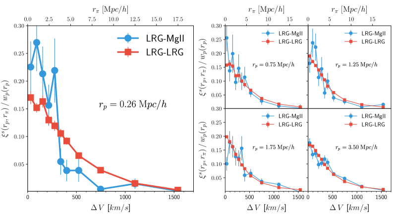
Figure 4: Comparison between the $\xi(r_{p},r_{\pi})/w_{p}(r_{p})$ profiles of LRG–MgII cross–correlation (blue circles) and LRG auto–correlation (red squares), within the LRG haloes (left main panel; $r_{p}{=}0.26\,h^{-1}\mathrm{Mpc}$) and on large scales beyond the 1–halo regime (right panels; $r_{p}{=}[0.75,1.25,1.75,3.50]\,h^{-1}\mathrm{Mpc}$), respectively. For each panel, the bottom and upper x–axes indicate the LOS separation using the relative velocity $\Delta V$ and the LOS distance $r_{\pi}$, respectively. The two sets of profiles closely track each other at large $r_{p}$ (right panels), but differ significantly at $r_{p}{=}0.26$ (left panel), where a sharp truncation occurs at $\Delta V{\sim}300\,\mathrm{km}\,s^{-1}$ (i.e., $r_{\pi}{\sim}0.34\,h^{-1}\mathrm{Mpc}$) in the LRG–MgII cross–correlation but not in the LRG auto–correlation.

To look more closely into the small–scale differences in RSD, we calculate the ratio between $\xi^{s}(r_{p},r_{\pi})$ and $w_{p}(r_{p})$ at fixed $r_{p}$, and compare the two sets of ratios as functions of $r_{\pi}$ in Figure 4. In essence, the $\xi^{s}(r_{p},r_{\pi})/w_{p}(r_{p})$ ratio profiles measure the redshift–space LOS probability distribution function of clouds or galaxies around LRGs at any $r_{p}$. In the left panel of Figure 4, we compare the ratio profiles of the LRG–MgII cross–correlation (blue circles) and LRG auto–correlation (red squares) at $r_{p}{\simeq}0.26\,h^{-1}\mathrm{Mpc}$ (i.e., $0.01\,h^{-1}\mathrm{Mpc}<r_{p}<0.5\,h^{-1}\mathrm{Mpc}$). We limit our lowest $r_{p}$ bin below $r_{p}{=}0.5\,h^{-1}\mathrm{Mpc}$ because we want to focus exclusively on the so–called “1-halo” term of the correlation signals — the typical halo radius of the LRG host haloes is estimated to be ${\sim}0.5{-}0.6\,h^{-1}\mathrm{Mpc}$ from either fitting to the stacked MgII absorption profiles (Zhu et al., 2014) or the weak lensing of massive quiescent galaxies (Mandelbaum et al., 2016; Zu & Mandelbaum, 2016). We also compare the two sets of ratio profiles computed at larger projected distances, $r_{p}{=}[0.75,1.25,1.75,3.50]\,h^{-1}\mathrm{Mpc}$, in the four right panels. In each panel, we label the bottom x–axis using the widely–used relative velocity $\Delta V$, while showing the redshift–space LOS distance $r_{\pi}$ in the upper x–axis.

The four right panels of Figure 4 indicate that the LOS distribution of MgII absorbers is in good agreement with that of galaxies at $r_{p}{>}0.6\,h^{-1}\mathrm{Mpc}$, i.e., in the “2–halo” regime. This is unsurprising, because the cool clouds should follow the distribution of galaxies on large scales regardless of wind or no–wind origins. Within the LRG haloes (left panel of Figure 4), however, the LOS distribution of MgII absorbers is drastically different from that of galaxies, exhibiting a sharp truncation at $\Delta V{\sim}300\,\mathrm{km}\,s^{-1}$ (i.e., $r_{\pi}{\sim}3.4\,h^{-1}\mathrm{Mpc}$). This sharp truncation explains the missing of FOG effect in the RSD of MgII absorbers, and can not be reproduced simply by reducing the velocity dispersion of the cool clouds (as will be demonstrated later in § 5). We note that the luminous red satellites do not exhibit the typical satellite kinematics within the LRG haloes — they are subject to stronger dynamic friction and likely had an earlier infall, therefore travelling more slowly than the avearge satellites. We thus expect the cross–correlation between the LRGs and typical galaxies would produce an even stronger FOG effect than the LRG auto–correlation. We also note that Kauffmann et al. (2017) also measured the redshift–space cross–correlation function between the CMASS LRGs and MgII absorbers. However, they used a different method of generating random catalogues, a different estimator than Equation 1, and a different binning, so it is difficult to make direct comparison between Figure 4 and their results. To extract the kinematic information encoded in the $\xi_{\mathrm{\tt{LRG-MgII}}}^{s}$ profile at $r_{p}{=}0.26\,h^{-1}\mathrm{Mpc}$, in the next step we will reconstruct the real–space LOS distribution of MgII absorbers around the LRGs from the measurements of $w_{p}(r_{p})$.

4 Spatial Distribution of Cool Clouds Around LRGs

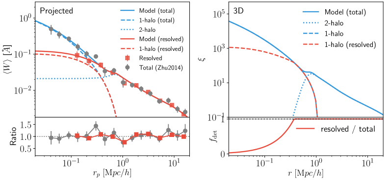
Figure 5: Left panel: Projected EW profiles of MgII absorbers around LRGs. Gray circles with errorbars are the measurements of the total absorption from stacked quasar spectra by Zhu et al. (2014), while red squares with errorbars indicate our measurements from the projected cross–correlation function between LRGs and the resolved MgII absorbers. Solid curves are the best–fitting predictions for the total (blue) and resolved (red) absorption signals, with dashed and dotted curves indicating the 1–halo and 2–halo components, respectively. The ratio profiles between the data measurements and best-fitting predictions are shown in the bottom panel for the total (gray circles) and resolved (red squares) absorption signals, respectively. Right panel: Similar to the left panel, but for the 3D isotropic cross–correlation functions between LRGs and MgII absorbers. The bottom panel shows the predicted radius dependence of absorber detection fraction in the Zhu & Ménard (2013) catalogue.

4.1 Predict Projected EW Profile $\mathbf{\left\langle W\right\rangle(r_{p})}$

Zhu et al. (2014) measured the projected MgII EW profile around the same sample of LRG galaxies, from the flux decrements induced in the stacked quasar spectra by MgII absorbers at the redshifts of the foreground LRGs. The (Zhu et al., 2014) profile is subsequently confirmed by other stacked MgII absorption measurements (also see Pérez-Ràfols et al., 2015; Lan & Mo, 2018), and is roughly consistent with the stacked H$\alpha$ emission measurements, suggesting the metal absorption and H$\alpha$ emission likely originate from the same CGM gas (Zhang et al., 2016; Zhang, Zaritsky, & Behroozi, 2018). The stacked signal of Zhu et al. (2014) is analogous to our measurement of the projected cross–correlation between LRGs and MgII absorbers $w_{p}(r_{p})$, but with one key difference. That is, by stacking the quasar spectra, Zhu et al. (2014) included the contribution from all the MgII absorbers, while our $w_{p}$ measurement only includes the spectrally resolved absorbers. Comparing to our method, the stacking technique is more useful for characterizing the total gas mass density profile, but at the expense of the individual redshifts of gas clouds, therefore less useful for inferring cloud kinematics. To reconstruct the spatial distribution of the resolved MgII absorbers, we will utilize the stacked absorption signal to infer the total gas density profile, which can be separated into contributions from the non-resolved vs. resolved MgII absorbers by fitting to the $w_{p}$ measurement assuming a radius–dependent detection fraction of the resolved absorbers.

To facilitate our joint analysis with the stacked MgII EW profile measured by Zhu et al. (2014), we convert our $w_{p}(r_{p})$ measurement into a projected MgII EW profile $\left\langle W\right\rangle$,

$$\left\langle W\right\rangle(r_{p})=w_{p}(r_{p})\frac{\mathrm{d}W}{\mathrm{d}r_{\pi}},$$ (4)

where $\mathrm{d}W/\mathrm{d}r_{\pi}$ is the average EW of MgII absorption per $h^{-1}\mathrm{Mpc}$ along the LOS. Ideally, this quantity should be computed by summing the EWs of all the MgII absorbers within the redshift range probed. However, the Zhu & Ménard (2013) MgII absorber catalogue suffers severe incompleteness at the low EW end, and an extra redshift–dependent incompleteness due to strong sky lines and sensitivity variation of the SDSS spectrographs. Therefore, we empirically infer the value of $\mathrm{d}W/\mathrm{d}r_{\pi}{=}2.6\times 10^{-4}\,h\mbox{\AA}/\mathrm{Mpc}$, from the ratio between the stacked MgII EW profile measured by Zhu et al. (2014) and our measurement of $w_{p}$ on scales beyond $3\,h^{-1}\mathrm{Mpc}$.

The left panel of Figure 5 compares the $\left\langle W\right\rangle$ profiles inferred from $w_{p}$ via Equation 4 (red squares) and from the stacking technique of Zhu et al. (2014) (gray circles). The two measurements are roughly consistent on scales above $0.5\,h^{-1}\mathrm{Mpc}$ — this is by design because we have adjusted the value of $\mathrm{d}W/\mathrm{d}r_{\pi}$ to match the two. However, the two profiles start to diverge below $0.5\,h^{-1}\mathrm{Mpc}$. In particular, the $w_{p}$–inferred $\left\langle W\right\rangle$ of resolved absorbers exhibits a flat trend with decreasing $r_{p}$, while the stacked $\left\langle W\right\rangle$ of total absorption is consistent with a projected NFW (Navarro-Frenk-White; Navarro et al., 1997) profile (Zhu et al., 2014). The discrepancy between the two $\left\langle W\right\rangle$ profiles on small scales implies that there is a radius-dependent detection inefficiency of the Zhu & Menard catalogue, so that MgII absorbers that are closer to the LRGs are less likely to be detected. At fixed EW, the close proximity of quasar sightlines to LRGs shoud not affect the detection probability of MgII absorbers, because the scattered light from the LRGs into the quasar fibres is minimal. We speculate that the radius-dependent inefficiency is induced by the fact that the average EW of the MgII absorbers decreases from the outer CGM to the center of the LRGs. Since the detection probability decreases rapidly at $\mathrm{EW}<2\mbox{\AA}$ (see figure 7 of Zhu & Ménard (2013)), the stacked MgII absorption profile is much steeper than the number density profile of the resolved MgII absorbers. The overall shape of our $w_{p}$–inferred $\left\langle W\right\rangle$ profile is consistent with the excess absorber number density profile measured by Anand, Nelson, & Kauffmann (2021), who utilized a larger MgII absorber catalogue derived from the SDSS DR16.

For the purpose of our analysis, it is more convenient to work with correlation functions than density profiles. Therefore, instead of reconstructing the radial number density profile of MgII absorbers $n(r)$, we focus on the “1–halo” component of the 3D isotropic cross–correlation function between the LRGs and absorbers $\xi_{1h}(r)$. The two are related via

$$\xi_{1h}(r)=\frac{n(r)-\overline{n}}{\overline{n}},$$ (5)

where $\overline{n}$ is the mean number density of cool clouds.

Following Zhu et al. (2014), we assume that the total cool gas distribution follows the dark matter distribution within haloes, which we model as

$$\xi_{1h}^{\mathrm{gas}}(r)\equiv\xi_{1h}^{\mathrm{dm}}(r)=\frac{\rho_{\mathrm{NFW}}(r\mid M_{h},c)}{\rho_{m}}f_{\mathrm{trans}}(r)-1,$$ (6)

where $\rho_{\mathrm{NFW}}(r\mid M_{h},c)$ is the NFW density profile of a dark matter halo with halo mass $M_{h}$ and concentration $c$, $\rho_{m}$ is the mean density of the Universe, and $f_{\mathrm{trans}}$ describes the so–called “spashback” transition near the halo boundary (Diemer & Kravtsov, 2014),

$$f_{\mathrm{trans}}(r)=\left[1+\left(\frac{r}{1.495\,r_{200m}}\right)^{4}\right]^{-2}.$$ (7)

We emphasize that although the result from Zhu et al. (2014) shows that an NFW profile provides an adequate description of the average cool gas density profile, the spatial distribution of the cool gas clouds in individual haloes could deviate significantly from the dark matter, depending on the dynamical state of the cool gas. For example, Wild et al. (2008) discovered that quasars could destroy MgII absorbers up to comoving distances of ${~{}}800$ $kpc$ along their lines of sight, so that the spatial distribution of cool clouds could depend strongly on the duty cycle of the supermassive blackholes in the galactic centre. However, it is plausible that the gas density profiles averaged over many haloes of various dynamical states may converge to an NFW–like profile. This possibility can be tested in the future against the increasingly fine-grained hydrodynamic simulations of the CGM (Peeples et al., 2019; Hafen et al., 2019; Suresh et al., 2019; Hummels et al., 2019; Fielding et al., 2020).

For describing the resolved MgII absorbers in our sample, we further include a radius–dependent inefficiency

$$\xi_{1h}(r)=\frac{\rho_{\mathrm{NFW}}(r\mid M_{h},c)}{\rho_{m}}f_{\mathrm{trans}}(r)f_{\mathrm{det}}(r)-1,$$ (8)

where $f_{\mathrm{det}}$ is the detection fraction

$$f_{\mathrm{det}}(r)=\left(\frac{r}{\kappa\,r_{200m}}\right)^{\alpha},$$ (9)

and we set $f_{\mathrm{det}}$ to be unity when $r{>}\kappa\,r_{200m}$.

We model the “2–halo” component of the 3D isotropic LRG–MgII cross–correlation as

$$\xi_{2h}(r)=b_{g}b_{c}\xi_{mm}(r)f_{\mathrm{ex}}(r),$$ (10)

where $\xi_{mm}$ is the dark matter auto–correlation function. Since we do not need to distinguish between $b_{g}$ and $b_{c}$, we merge them to form a single parameter $b{\equiv}b_{g}b_{c}$. The last term on the right-hand side, $f_{\mathrm{ex}}(r)$, describes the so–called “halo exclusion” effect, which arises from the fact that the centre of one halo cannot sit within the virial radius of another. In particular, $f_{\mathrm{ex}}(r)$ is unity at $r{>}r^{\mathrm{max}}_{200m}$, as there is no halo exclusion when the distance is larger than twice the radius of the largest haloes $r^{\mathrm{max}}_{200m}$. By the same token, $f_{\mathrm{ex}}(r)$ declines to zero at some characteristic distance that corresponds to twice the radius of the smallest haloes.

For analytically solving for $f_{\mathrm{ex}}$ at any given distance, we need to explicitly integrate over all pairs of haloes that are too small to run into each other when separated by that distance(e.g., see equation B10 of Tinker et al., 2005). However, such analytic calculation can only be performed if the halo occupation distributions (HODs) of both the LRGs and MgII absorbers are assumed a priori. Since a comprehensive HOD modelling of the MgII absorbers is beyond the scope of this paper, for our first–cut analysis we choose to use a simple error function to mimic the behavior of halo exclusion

$$f_{\mathrm{ex}}(r)=\frac{1}{2}\left[1+\mathrm{erf}\left(\frac{r-\beta\,r_{200m}}{\sigma_{\mathrm{ex}}}\right)\right],$$ (11)

where $\beta\,r_{200m}$ is the characteristic scale above which $f_{\mathrm{ex}}$ asymptotes to unity, and $\sigma_{\mathrm{ex}}$ describes the width of the transition of $f_{\mathrm{ex}}$ from unity to zero, which depends on the widths of the halo mass distributions of the LRGs and MgII absorbers. We have verified that for the HOD of a typical stellar–mass thresholded sample in (Zu & Mandelbaum, 2015), the analytic halo exclusion profile can be reasonably well described by Equation 11.

We derive the overall $\xi(r)$ signals by directly summing the two components, so that

$$\xi^{\mathrm{gas}}(r)=\xi_{1h}^{\mathrm{gas}}(r)+\xi_{2h}(r),$$ (12)

for the LRG–gas cross–correlation, and

$$\xi(r)=\xi_{1h}(r)+\xi_{2h}(r),$$ (13)

for the LRG–MgII absorbers cross–correlation, respectively. Note that we adopt the same “2–halo” component for the total and resolved absorption, assuming that the EW–dependence of cloud bias $b_{c}$ is weak (Tinker & Chen, 2008; Gauthier et al., 2009). Finally, we integrate the $\xi$ profiles along the LOS to obtain $w_{p}(r_{p})$ via Equation 3, and then multiply by $\mathrm{d}W/\mathrm{d}r_{\pi}$ to predict the $\left\langle W\right\rangle(r_{p})$ profiles.

4.2 Reconstruct 3D Galaxy–cloud Cross–correlation

In total, we have seven free parameters, including $\{M_{h},c,b,\kappa,\alpha,\beta,\sigma_{\mathrm{ex}}\}$. We perform simple $\chi^{2}$–minimization fitting to the observed total and resolved $\left\langle W\right\rangle$ profiles, using the diagonal errors provided by Zhu et al. (2014) for the stacked signal and the full covariance matrix measured from Jackknife re-sampling for the resolved profile, respectively. We enforce the 2–halo term to be zero at $r{<}0.2h^{-1}\mathrm{Mpc}$ during the fit, in order to eliminate the false solution that artificially boosts the 2–halo term on very small scales to fit the data. We find the best–fitting values to be $\{\lg\,M_{h}{=}13.19,c{=}5.1,b{=}1.15,\kappa{=}0.63,\alpha{=}1.2,\beta{=}1.15,\sigma_{\mathrm{ex}}{=}0.14\}$, and the best–fitting predictions of the total (blue solid) and resolved (red solid) signals are shown in the left main panel of Figure 5. The bias value is slightly higher than predicted for haloes with $\lg\,M_{h}{=}13.19$, probably because a good fraction of the LRGs are satellite galaxies inside massive haloes (Zu, 2020). Both predictions are in excellent agreement with the measurements, as demonstrated by the ratios between data and predictions in the left bottom panel of Figure 5.

In many observations, MgII absorbers detected at small impact parameters ($r_{p}{<}0.2\,h^{-1}\mathrm{Mpc}$) to a foreground galaxy are usually considered part of the CGM of that galaxy, but some of them should be interlopers from other galaxies, i.e., part of the “2–halo” component. To obtain an estimate of the interloper fraction, we show the best-fitting 1–halo components of the total (blue dashed) and resolved (red dashed) absorption in the left panel of Figure 5. For the stacked measurement, the strong absorption signal at $r_{p}{<}0.2\,h^{-1}\mathrm{Mpc}$ is almost entirely contributed by the gas clouds within the LRG haloes (i.e., the blue dashed curve is much higher than the blue dotted curve). For the resolved absorbers, however, ${\sim}1/3{-}1/5$ of the strong MgII absorbers with impact parameters (${<}0.2\,h^{-1}\mathrm{Mpc}$) are interlopers from the CGM of other galaxies (compare the red dashed curve with the blue dotted curve). This is roughly consistent with the expectation from hydrodynamic simulations, where Ho et al. (2020) found that a ${\pm}500\,\mathrm{km}\,s^{-1}$ cut by ${v}_{\mathrm{los}}$ could include many gas clouds physically outside of the virial radius. Fortunately, our cross–correlation method is able to statistically remove the impact of those interloper on our analysis.

In the right panel of Figure 5, we show the best–fitting 3D isotropic cross–correlation functions for the total signal (blue solid), which is further decomposed into 1–halo (blue dashed; Equation 6) and 2–halo (blue dotted; Equation 10) components; The 1–halo component of the best–fitting $\xi$ profile of the resolved clouds is indicated by the red dashed curve (Equation 8). In the bottom sub-panel, we show the best–fitting profile of $f_{\mathrm{det}}$, indicating that the relatively flat trend of $\left\langle W\right\rangle(r_{p})$ below $r_{p}{\sim}0.3\,h^{-1}\mathrm{Mpc}$ is due to the cancellation of the steep increase in total gas density by the rapid decline of detection sensitivity toward small radii.

4.3 Subtract Two–halo Term from $\mathbf{\xi_{\mathrm{\tt{LRG-MgII}}}^{s}}$

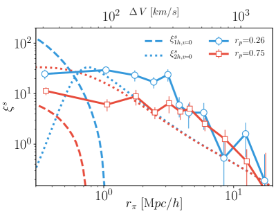
Figure 6: Comparison between the redshift–space LRG–MgII cross–correlation functions at $r_{p}{=}0.26\,h^{-1}\mathrm{Mpc}$ (blue) vs. $r_{p}{=}0.75\,h^{-1}\mathrm{Mpc}$ (red). Circles (squares) with errorbars are the observed $\xi^{s}$ at $r_{p}{=}0.26$ ($r_{p}{=}0.75$). Dashed and dotted curves indicate the 1–halo and 2–halo components of $\xi^{s}(r_{\pi}|r_{p})$, respectively, predicted from $\xi(r{=}\sqrt{r_{p}^{2}{+}r_{\pi}^{2}})$, i.e., assuming zero peculiar velocities. We expect the 2–halo component of the observed $\xi^{s}$ signal at $r_{p}{=}0.26$ can be well approximated by the $\xi^{s}$ signal observed at $r_{p}{=}0.75$.

The kinematics of cool clouds within the LRG haloes is encoded in the redshift–space cross–correlation function between the LRGs and MgII absorbers $\xi_{\mathrm{\tt{LRG-MgII}}}^{s}$ at small $r_{p}$. From the modelling of $w_{p}$ we infer that the typical radius of the LRG haloes is ${\sim}0.6\,h^{-1}\mathrm{Mpc}$ (for haloes with $\lg\,M_{h}{=}13.19$). Therefore, we will focus on the average RSD signal measured between $r_{p}{=}0.01\,h^{-1}\mathrm{Mpc}$ and $0.5\,h^{-1}\mathrm{Mpc}$, i.e., $\xi^{s}(r_{\pi}|r_{p}{=}0.26\,h^{-1}\mathrm{Mpc})$.

Ideally, one would model the full RSD signal on both small and large $r_{\pi}$, i.e., including both the 1–halo and 2–halo components of $\xi_{\mathrm{\tt{LRG-MgII}}}^{s}$ at $r_{p}{=}0.26\,h^{-1}\mathrm{Mpc}$, as was previously done in, e.g., Zu & Weinberg (2013). However, since we are only concerned with the CGM kinematics inside the haloes, we will isolate the 1–halo term of the $\xi_{\mathrm{\tt{LRG-MgII}}}^{s}$ signal by subtracting the 2–halo term from the full RSD signal observed at $r_{p}{=}0.26\,h^{-1}\mathrm{Mpc}$. The isolated 1–halo RSD can then be modelled as the convolution between $\xi_{1h}$, the quantity we have reconstructed in  § 4.2, and the LOS velocity distribution of the cool clouds, the quantity we want to infer in this paper.

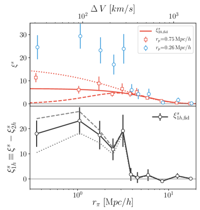
Figure 7: Top panel: Blue circles and red squares are the redshift–space LRG–MgII cross–correlation functions measured at $r_{p}{=}0.26\,h^{-1}\mathrm{Mpc}$ and $0.75\,h^{-1}\mathrm{Mpc}$, respectively. Red solid curve is our fiducial prediction of $\xi^{s}_{2h}$ from the best–fitting powered exponential function (Equation 14). Red dotted and dashed curves are the upper and lower bounds of $\xi^{s}_{2h}$, respectively, inferred from adjusting the small–scale slope parameter of Equation 15. Bottom panel: The 1–halo components of $\xi^{s}(r_{\pi}|r_{p}{=}0.26\,h^{-1}\mathrm{Mpc})$, obtained by subtracting the predicted $\xi^{s}_{2h}$ curves shown in the top panel from the observed signal at $r_{p}{=}0.26\,h^{-1}\mathrm{Mpc}$. Black circles with errorbars indicate our fiducial estimate of the $\xi^{s}_{1h}(r_{\pi}|r_{p}{=}0.26\,h^{-1}\mathrm{Mpc})$ profile.

Accurate subtraction of the 2–halo term requires theoretically modelling the large-scale infall of cool clouds outside the halo radius, which is highly challenging and therefore beyond the scope of this paper. For a first–cut analysis, we derived the 2–halo term $\xi^{s}_{2h}(r_{\pi}|r_{p}{=}0.26\,h^{-1}\mathrm{Mpc})$ empirically, by making use of the RSD signal observed at $r_{p}{=}0.75\,h^{-1}\mathrm{Mpc}$. The rationale is as follows. Firstly, without the peculiar velocities, the cross–correlation function along the LOS is simply $\xi^{s}_{v{=}0}(y|r_{p})=\xi(\sqrt{y^{2}{+}r_{p}^{2}})$. Since $\xi(r)$ is a slow–varying function of $r$ on large scales, the underlying cloud distribution along the LOS should be similar between $r_{p}{=}0.26$ and $0.75$ for $y{\gtrsim}2\,h^{-1}\mathrm{Mpc}$. Secondly, the LOS velocity distribution is the projection of the isotropic 2D velocity distribution along the LOS. The two average “sightlines” at $r_{p}{=}0.26\,h^{-1}\mathrm{Mpc}$ and $0.75\,h^{-1}\mathrm{Mpc}$ are almost parallel at the mean redshift of the LRG sample ($z{\sim}0.55$), differing only by 1 arc min. Therefore, the LOS velocity distributions of clouds beyond the halo radius should be almost the same between the two $r_{p}$ bins. Combining the two factors together, we expect that the 2–halo components of the redshift–space cross–correlation signals are similar between the two adjacent $r_{p}$ bins at $0.26\,h^{-1}\mathrm{Mpc}$ and $0.75\,h^{-1}\mathrm{Mpc}$.

Figure 6 illustrates the rationale behind our expectation that the two adjacent $r_{p}$ bins should share similar 2–halo terms of the RSD signal around LRGs. The dashed and dotted curves indicate the 1–halo and 2–halo contributions to $\xi^{s}_{v{=}0}(r_{\pi}|r_{p})$, predicted by the best–fitting $\xi(r)$ in the absence of peculiar velocities, at $r_{p}{=}0.26\,h^{-1}\mathrm{Mpc}$ (blue) and $0.75\,h^{-1}\mathrm{Mpc}$ (red), respectively. Circles with errorbars are the measured redshift–space correlation functions $\xi_{\mathrm{\tt{LRG-MgII}}}^{s}$ for the two $r_{p}$ bins (also shown in Figure 4). Unsurprisingly, the 1–halo term (dashed blue curve) at $r_{p}{=}0.26\,h^{-1}\mathrm{Mpc}$ is ${\sim}20$ times higher than that at $r_{p}{=}0.75\,h^{-1}\mathrm{Mpc}$ (dashed red curve), driving the strong tophat–like enhancement of the observed redshift–space correlation on scales below $r_{\pi}{\simeq}4\,h^{-1}\mathrm{Mpc}$ (i.e., $\Delta V{\simeq}300\,\mathrm{km}\,s^{-1}$) for the $r_{p}{=}0.26\,h^{-1}\mathrm{Mpc}$ bin. Furthermore, the 2–halo terms of the two $r_{p}$ bins are indeed comparable when peculiar velocities are turned off (dotted curves). More important, the observed redshift–space correlations of the two $r_{p}$ bins are highly consistent with each other at $r_{\pi}{>}4\,h^{-1}\mathrm{Mpc}$. This consistency is very encouraging — the underlying 2–halo component of the observed $\xi_{\mathrm{\tt{LRG-MgII}}}^{s}$ signal at $r_{p}{=}0.26$ (blue circles) should be well approximated by the total observed $\xi_{\mathrm{\tt{LRG-MgII}}}^{s}$ signal at $r_{p}{=}0.75$ (red squares).

Therefore, in order to estimate the underlying 1–halo term at $r_{p}{=}0.26\,h^{-1}\mathrm{Mpc}$, we fit an analytic curve to the total observed $\xi_{\mathrm{\tt{LRG-MgII}}}^{s}$ signal at $r_{p}{=}0.75\,h^{-1}\mathrm{Mpc}$ and subtract it from the total observed signal at $r_{p}{=}0.26\,h^{-1}\mathrm{Mpc}$. Zu & Weinberg (2013) discovered that the $\xi^{s}(r_{\pi}|r_{p})$ profiles can be well described by a powered exponential function

$$\xi^{s}(r_{\pi}|r_{p})=\xi^{s}_{0}\exp\left\{-\left|\frac{r_{\pi}}{r_{\pi,c}}\right|^{\beta}\right\},$$ (14)

where $r_{\pi,c}$ is the characteristic $r_{\pi}$ at which $\xi^{s}$ declines to $1/e$ of its maximum value $\xi^{s}_{0}$ at $r_{\pi}{=}0$, and $\beta$ is the shape parameter that controls the rate of the decline. We apply Equation 14 to the RSD signal at $r_{p}{=}0.75\,h^{-1}\mathrm{Mpc}$, and the results are shown in Figure 7.

In the top panel of Figure 7, blue circles (red squares) with errorbars are the observed total $\xi_{\mathrm{\tt{LRG-MgII}}}^{s}$ signals at $r_{p}{=}0.26\,(0.75)\,h^{-1}\mathrm{Mpc}$. Red solid curve is the prediction from Equation 14 using the best–fitting parameters of $r_{\pi,c}{=}6.71$, $\beta{=}1.36$, and $\xi^{s}_{0}{=}41.67$. We omit the data point from the lowest $r_{\pi}$ bin during the fit, where we expect a relatively larger discrepancy between the 2–halo term at $r_{p}{=}0.26\,h^{-1}\mathrm{Mpc}$ and the observed signal at $r_{p}{=}0.75\,h^{-1}\mathrm{Mpc}$ than other $r_{\pi}$ bins (see Figure 6). We also show two other model curves (dotted and dashed) in which we use a different function form

$$\xi^{s}(r_{\pi}|r_{p})=\xi^{s}_{0}\left|\frac{r_{\pi}}{r_{\pi,c}}\right|^{\alpha}\exp\left\{-\left|\frac{r_{\pi}}{r_{\pi,c}}\right|^{\beta}\right\},$$ (15)

where the extra parameter $\alpha$ modifies the slope at small $r_{\pi}$. We adjust the two model fits so that the dashed and dotted curves roughly delineate the lower and upper bounds of the observed data points at $r_{\pi}{<}5\,h^{-1}\mathrm{Mpc}$, respectively.

We show the derived 1–halo components of the $\xi_{\mathrm{\tt{LRG-MgII}}}^{s}$ at $r_{p}{=}0.26\,h^{-1}\mathrm{Mpc}$ in the bottom panel of Figure 7, by subtracting each of the three model curves of $\xi_{2h}^{s}$ shown in the top panel from the observed $\xi_{\mathrm{\tt{LRG-MgII}}}^{s}$ data points. Circles with errorbars represent our fiducial estimates for $\xi^{s}_{1h}(r_{\pi}|r_{p}{=}0.26)$, obtained from the subtraction of the best fit using Equation 14, while the dashed and dotted curves from the subtraction of the respective curves predicted by Equation 15. We emphasize that, despite the large discrepancies in $\alpha$, all three estimates of $\xi^{s}_{1h}$ exhibit a sharp truncation at $r_{\pi}{\sim}3{-}4\,h^{-1}\mathrm{Mpc}$, echoing the missing–FOG effect seen in Figure 3. This also suggests that the sharp truncation is physical, and most likely driven by some kinematic feature in the velocity distribution of cool clouds. In the next section, we will describe the fiducial measurements of $\xi^{s}_{1h}(r_{\pi}|r_{p}{=}0.26)$ (black open circles with errorbars in the bottom panel of Figure 7) using four different cloud kinematic models. For our first–cut analysis, we directly apply the Jackknife uncertainties of $\xi^{s}(r_{\pi}|r_{p}{=}0.26\,h^{-1}\mathrm{Mpc})$ for the error matrix of the fiducial measurements, i.e., assuming zero uncertainty from the subtraction of the 2–halo term. Despite that the errorbars are underestimated, they are roughly consistent with the allowed range sandwiched between the lower and upper bounds, indicated by the gray dotted and dashed curves, respectively.

5 Comparison of Cloud Kinematic Models

Armed with the 1–halo components of the 3D real–space ($\xi_{1h}(r)$) and redshift–space ($\xi^{s}_{1h}(r_{\pi}|r_{p}{=}0.26\,h^{-1}\mathrm{Mpc})$; hereafter shortened as $\xi^{s}_{1h}(r_{\pi})$) cross–correlation functions between the LRGs and MgII absorbers, we now investigate different cloud kinematic models by examining their predicted RSD signals and comparing to the observations. In particular, we compute $\xi^{s}_{1h}$ by convolving $\xi_{1h}(r)$ with the LOS velocity distribution predicted by each kinematic model

$$\xi^{s}_{1h}(r_{\pi}\mid r_{p}) = \frac{H_{z}}{1+z}\int_{-\infty}^{+\infty}\left[\xi_{1h}\big{(}\sqrt{r_{p}^{2}+y^{2}}\big{)}\right]\times\;\;\;\;\;\;\;\;\;\;\;\;\;\;$$ (16)

$$p\big{(}{v}_{\mathrm{los}}{=}\frac{H_{z}}{1+z}\left(r_{\pi}-y\right)\mid r_{p},y,\bm{\theta}\big{)}\,\mathrm{d}y,$$

where $r_{p}{=}0.26\,h^{-1}\mathrm{Mpc}$, $p({v}_{\mathrm{los}}|r_{p},y,\bm{\theta})$ is the LOS velocity distribution of cool clouds at fixed $y$, and $\bm{\theta}$ is the parameter set of each kinematic model.

Following the discussion in § 1, we consider four different kinematic models:

• Isothermal model described by a single LOS velocity dispersion ${\sigma}_{\mathrm{los}}$.

• Satellite infall model in which the MgII absorbers reside in the CGM of satellite galaxies and follow the motion of satellite infall.

• Cloud accretion model in which clouds follow the cosmological gas accretion as prescribed by Afruni et al. (2019).

• Tired wind model in which ancient wind bubble “hangs” in the outer halo, inspired by the semi–analytic model of Lochhaas et al. (2018).

Among the four models, the first three are no–wind models that assume random or inflowing motion of the clouds, while the last one assumes outflowing clouds. Although our ultimate goal is to distinguish the four kinematic models, the current measurement uncertainties of $\xi^{s}_{1h}$ are quite large (${\sim}30{-}40\%$ on scales below $3\,h^{-1}\mathrm{Mpc}$), rendering any $\chi^{2}$–based model comparison highly inconclusive. Nonetheless, we will compute the Akaike Information Criterion (AIC) value for each best–fitting model as AIC$=2k{+}\chi^{2}$, where $k$ is the number of model parameters, and compare the AIC of the four models.

More important, we will assess the capability of each model to reproduce the sharp truncation of the observed $\xi^{s}_{1h}$ profile at $r_{\pi}{\sim}3.4\,h^{-1}\mathrm{Mpc}$, i.e., the missing–FOG effect in the RSD of MgII absorbers around LRGs. Despite the large statistical uncertainties in individual $r_{\pi}$ bins, the truncation feature itself is robust — the observed $\xi^{s}_{1h}$ profile stays roughly constant below $r_{\pi}{\sim}3\,h^{-1}\mathrm{Mpc}$, but drops rapidly from $16.9{\pm}5.8$ at $r_{\pi}{=}3.15\,h^{-1}\mathrm{Mpc}$ to $1.2{\pm}2.6$ at $r_{\pi}{=}3.85\,h^{-1}\mathrm{Mpc}$. We will describe each model in turn below.

5.1 Isothermal

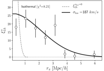
Figure 8: Comparison of the observed 1–halo components of the LRG–MgII absorber redshift–space cross–correlation function $\xi_{1h}^{s}$ (circles with errorbars) with the best–fitting prediction by the isothermal model (solid curve). The $\chi^{2}$ value is indicated in the top left corner. Dashed line shows the predicted signal when peculiar velocity is off.

The isothermal model was implicitly assumed in many CGM studies, where a velocity dispersion was usually computed from the $\Delta V$ distribution and compared to the virial or escape velocity of the haloes. Similarly, we model $p({v}_{\mathrm{los}})$ as a Gaussian distribution with zero mean and dispersion ${\sigma}_{\mathrm{los}}$, and predict the $\xi^{s}_{1h}$ profile by convolving $p({v}_{\mathrm{los}})$ with our reconstructed $\xi_{1h}(r)$ profile via Equation 16. We derive the best–fitting value of ${\sigma}_{\mathrm{los}}$ via $\chi^{2}$ minimization. Figure 8 compares the best–fitting prediction from the isothermal model (solid black curve) to the observed $\xi^{s}_{1h}$ profile (circles with errorbars). The best–fitting value of ${\sigma}_{\mathrm{los}}$ is $187\,\mathrm{km}\,s^{-1}$, lower than the virial LOS dispersion (${\simeq}247\,\mathrm{km}\,s^{-1}$ for $\lg\,M_{h}{=}13.19$) and consistent with the results from previous studies (e.g., Zhu et al., 2014; Huang et al., 2016; Anand, Nelson, & Kauffmann, 2021; Huang et al., 2021). The solid curve has a $\chi^{2}$ value of $8.21$, hence a statistically good fit to the eight data points. However, the model predicts a gradual decline of the $\xi_{1h}^{s}$ profile, without the sharp truncation seen in the data profile. This is unsurprising — the isothermal model can only stretch the relative redshift distribution of MgII absorbers around LRGs, but cannot produce a sharp feature in the distribution.

5.2 Satellite Infall

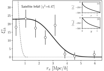
Figure 9: Similar to Figure 8, but for the satellite infall model. Inset panels (a) and (b) indicate the average radial and LOS velocity profiles predicted by the best–fitting model, respectively.

Many of the LRGs are the central galaxies of group–size haloes with halo mass above $10^{13}\,h^{-1}M_{\odot}$, which frequently accrete lower–mass systems that likely host star-forming galaxies that could drive cool clouds into the CGM via strong outflows. In this scenario, the observed MgII absorbers around LRGs are actually associated with the CGM of infalling satellite galaxies. Hydrodynamic simulations predict that it usually takes a couple Gyrs before the satellite galaxies become quenched after being accreted onto the larger halo (Simha et al., 2009; Wetzel et al., 2013). Therefore, we could model the cloud kinematics based on the velocity distribution of recently accreted satellites inside haloes.

After examining the galaxy infall kinematics in the Millennium simulation, Zu & Weinberg (2013) found that the average radial velocity of the infalling galaxies reaches maximum at some characteristic radius (${\sim}1\,h^{-1}\mathrm{Mpc}$) and then declines rapidly towards zero at the halo center. Therefore, we describe the radial velocity profile of cool clouds as

$$\left\langle v_{r}(r)\right\rangle=\left(\frac{r}{1.2}\right)^{\beta}v_{\mathrm{max}},$$ (17)

where $v_{\mathrm{max}}$ is the maximum radial velocity at $1.2\,h^{-1}\mathrm{Mpc}$, about twice the $r_{200m}$ of LRG haloes. We do not assume any rotational component in the cloud kinematics, which is more important for disky galaxies (Zabl et al., 2019; DeFelippis et al., 2021). Adopting an average projected distance of $r_{p}{=}0.26\,h^{-1}\mathrm{Mpc}$, we then convert the radial velocity profile $\left\langle v_{r}(r)\right\rangle$ to an average LOS velocity profile $\left\langle{v}_{\mathrm{los}}(y)\right\rangle$ and assume a constant LOS velocity dispersion ${\sigma}_{\mathrm{los}}$, yielding a simple satellite infall model with three parameters $\{v_{\mathrm{max}},\,\beta,\,{\sigma}_{\mathrm{los}}\}$. By minimizing the $\chi^{2}$, we obtain the best–fitting parameters as $v_{\mathrm{max}}{=}{-}479.0\,\mathrm{km}\,s^{-1}$, $\beta{=}0.42$, and ${\sigma}_{\mathrm{los}}{=}71.1\,\mathrm{km}\,s^{-1}$, respectively.

Figure 9 shows the best–fitting prediction from our satellite infall model (solid black curve), with the two inset panels indicating the best–fitting average radial (top) and LOS (bottom) velocity profiles, respectively. Compared to the isothermal model ($k{=}1$), the minimum $\chi^{2}$ decreases from $8.21$ to $6.47$ with two more parameters ($k{=}3$). On the one hand, based on the classical Akaike information criterion (AIC$=2k+\chi^{2}$), the satellite infall model has a slightly higher AIC value ($12.47$) than the isothermal model ($10.21$), hence a slightly less preferred model; But on the other hand, the satellite infall model produces a more flattened profile on small scales and a steeper decline, hence a better match to the shape of the $\xi^{s}_{1h}$ profile than the isothermal model. However, our satellite infall model still cannot reproduce the observed sharp truncation at $r_{\pi}{\sim}3.4\,h^{-1}\mathrm{Mpc}$.

5.3 Cloud Accretion

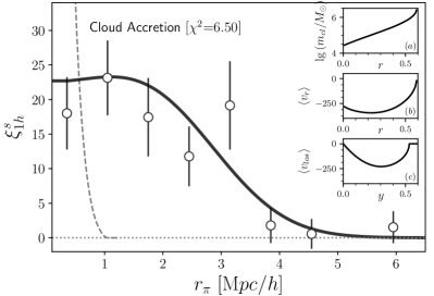
Figure 10: Similar to Figure 8, but for the cloud accretion model. Inset panels (a), (b), and (c) show the cloud mass evaporation, average radial velocity profile, and average LOS velocity profile, respectively.

Apart from infalling with the satellite galaxies, the observed cool clouds could also be part of the cosmological inflow that sustains the growth of LRG haloes. We adopt the same semi–analytic model of cloud accretion developed Afruni et al. (2019) to predict the radial and LOS velocity profiles of gas clouds; But instead of assuming a theoretical cool gas accretion rate as in Afruni et al. (2019), we convolve the LOS velocity distribution with our reconstructed $\xi_{1h}(r)$ profile to predict the $\xi^{s}_{1h}$ profile via Equation 16. In this way, our comparison with the observation is self–consistent, because both $\xi_{1h}(r)$ and $\xi^{s}_{1h}$ are derived from observations and the cloud kinematics is the only unknown in the problem. We will briefly describe the relevant components of the Afruni et al. (2019) model below and refer the reader to Afruni et al. (2019) for more technical details.

The Afruni et al. (2019) model describes the radial equation of motion of the cool clouds as

$$\frac{\mathrm{d}v_{r}}{\mathrm{d}r}=\frac{1}{v_{r}(r)}\frac{GM(<r)}{r^{2}}-\frac{\pi\,r^{2}_{cl}\,\rho_{\mathrm{cor}}(r)\,v_{r}(r)}{m_{cl}(r)},$$ (18)

where $M(<r)$ is the halo mass enclose within $r$, $\rho_{\mathrm{cor}}$ is the density of the hot corona gas, and $r_{cl}$ ($m_{cl}$) is the radius (mass) of a typical gas cloud. The second term on the r.h.s. of Equation 18 describes the deceleration of the cool clouds due to ram pressure drag, and $\rho_{\mathrm{cor}}$ is derived from the NFW potential by assuming hydrostatic equilibrium of the hot gas with the dark matter halo. The mass and radius of the gas cloud are related via

$$r_{cl}=\left(\frac{3m_{cl}}{4\pi\rho_{cl}}\right)^{1/3},$$ (19)

where $\rho_{cl}$ is the density of the cool clouds, calculated from assuming pressure equilibrium between the cool and hot phases of the CGM. Additionally, the mass loss due to hydrostatic instabilities (Armillotta et al., 2017) is modelled as

$$\frac{\mathrm{d}\,m_{cl}}{\mathrm{d}\,r}=-\alpha\frac{m_{cl}(r)}{v_{r}(r)},$$ (20)

where $\alpha$ is the cloud evaporation rate. Following Afruni et al. (2019), we assume all the clouds start with zero velocity at $r_{200m}{=}0.6\,h^{-1}\mathrm{Mpc}$ and initial cloud mass $m_{0,cl}$, and then glide through an LRG halo with $\lg\,M_{h}{=}13.19$. By combining Equations 18, 19, and 20 together, we can solve for the radial velocity profile $\left\langle v_{r}(r)\right\rangle$ of cool clouds for any given values of $\alpha$ and $m_{0,cl}$, hence the LOS velocity profile $\left\langle{v}_{\mathrm{los}}(y)\right\rangle$ at $r_{p}{=}0.26\,h^{-1}\mathrm{Mpc}$. Finally, assuming a constant LOS velocity dispersion ${\sigma}_{\mathrm{los}}$, we can predict the $\xi^{s}_{1h}$ profile from $\xi_{1h}(r)$ using Equation 16. By minimizing the $\chi^{2}$, we find the best–fitting parameters of the cloud accretion model to be $\alpha{=}2.10\,\mathrm{G}yr^{-1}$, $\lg\,m_{0,cl}{=}6.47$, and ${\sigma}_{\mathrm{los}}{=}98.5\,\mathrm{km}\,s^{-1}$, respectively. Compared to the constraints from Afruni et al. (2019), our mass loss rate is similar to theirs ($\alpha{=}1.8\,\mathrm{G}yr^{-1}$), but our cloud mass is larger by a factor of 30 ($\lg\,m_{0,cl}{=}4.85$). The cloud mass discrepancy is unsurprising because we rely only on the kinematics to infer $m_{cl}$ while Afruni et al. (2019) used both the velocity distribution and the hydrogen column densities.

Figure 10 shows the best–fitting prediction from the cloud accretion model (solid black curve), with the three inset panels indicating the best–fitting average mass evaporation (top), radial velocity (middle), LOS velocity (bottom) profiles, respectively. Despite significant differences in the predicted radial velocity profiles, the cloud accretion model is almost indistinguishable from the satellite infall model, with nearly the same values of minimum $\chi^{2}$ ($6.47$ vs. $6.50$) and the same number of parameters (hence similar AIC values $12.47$ vs. $12.50$). Meanwhile, similar to the satellite infall model, the cloud accretion model produces a flattened small–scale profile followed by a decline that is less sharp than seen in the data profile.

5.4 Tired Wind

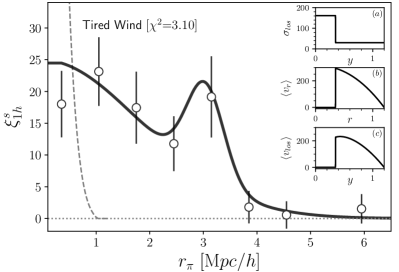
Figure 11: Similar to Figure 8, but for the tired wind model. Inset panels (a), (b), and (c) indicate the LOS velocity dispersion, average radial velocity, and average LOS velocity profiles, respectively.

The three no–wind models we have explored so far could all provide statistically good fits to the RSD data, but are unable to reproduce the sharp truncation in the observed $\xi^{s}_{1h}$ profile. In particular, the two inflow–based models could produce a similarly flattened profile on small scales, but the decline at $r_{\pi}{\sim}3{-}4\,h^{-1}\mathrm{Mpc}$ is not as steep as in the data profile. An outflow–based model may be able to obtain a better match by propagating a wind bubble to the outer CGM, as predicted by the model of  Lochhaas et al. (2018).

To mimic the kinematic features of ancient wind bubbles driven by the early star formation of LRGs, we adopt a simple “tired wind” prescription consisting of a dispersion–dominated component at small radii and a radially outflowing component at large radii. In particular, the radial velocity profile is

$$\left\langle v_{r}(r)\right\rangle = \left\{\begin{array}[]{ll}0&\quad\mbox{if $r<r_{\mathrm{min}}$ },\\ \left(1-\left(r/1.2\right)^{\gamma}\right)v_{0}&\quad\mbox{if $r\geqslant r_{\mathrm{min}}$ },\end{array}\right.$$

where $v_{0}$ is the launch velocity of the wind bubbles from the halo center and $r_{\mathrm{min}}$ is the minimum radius of the radiatively cooled wind bubble, driven by the last star formation episode of the LRGs before quenching. On scales below $r_{\mathrm{min}}$, we assume random motion with LOS velocity dispersion ${\sigma}_{\mathrm{los}}$ for the cool clouds, which could be formed via shell fragmentation due to various instabilities; On scales above $r_{\mathrm{min}}$, we assume a constant LOS velocity dispersion of $30\,\mathrm{km}\,s^{-1}$ for the outflow component. This choice of dispersion is small enough so that each wind bubble remains a coherent thin–shell without fragmentation, and large enough to avoid overfitting the data. Therefore, we have in total four parameters: $r_{\mathrm{min}}$, ${\sigma}_{\mathrm{los}}$, $v_{0}$, and $\gamma$, and their best–fitting values from $\chi^{2}$ minimization are $0.35\,h^{-1}\mathrm{Mpc}$, $161.0\,\mathrm{km}\,s^{-1}$, $317.0\,\mathrm{km}\,s^{-1}$, and $2.18$, respectively.

Figure 11 shows the best–fitting prediction from the tired wind model (solid black curve), with the three inset panels indicating the best–fitting LOS velocity dispersion (top), radial velocity (middle), and LOS velocity (bottom) profiles, respectively. The tired wind model provides an excellent description to the data with $\chi^{2}{=}3.1$ and a reasonable AIC value of $11.10$. Clearly, the significant improvement in $\chi^{2}$ from the other three models is mainly driven by the better match to the observed truncation of $\xi^{s}_{1h}$, thanks to the survived wind bubble moving at $250\,\mathrm{km}\,s^{-1}$ at $r{\sim}400\,h^{-1}\mathrm{kpc}$. This tired wind scenario is also roughly consistent with the theoretical expectation from the Lochhaas et al. (2018) model. While the Lochhaas et al. (2018) model tracks the radial motion of a single wind–bubble as a function of time for an individual galaxy, our radial velocity profile effectively describes the synthetic snapshot of a continuous series of wind–bubbles launched at different epochs by different galaxies.

Thus far, all the four best–fitting models we explored provide statistically good fits to the RSD of MgII absorbers around LRGs, yielding similar AIC values that render no particular model more preferable than the other three. However, if we focus on reproducing the truncation feature in the observed $\xi^{s}_{1h}$, the tired wind model clearly stands out, by interpreting the truncation as the kinematic signature of ancient wind bubbles.

6 Summary and Look to the Future

In this paper, we have measured the LRG–MgII absorber cross–correlation function in the redshift space and projected along the LOS, $\xi_{\mathrm{\tt{LRG-MgII}}}^{s}(r_{p},r_{\pi})$ and $w_{p}(r_{p})$, respectively. Compared to the LRG auto–correlation, $\xi_{\mathrm{\tt{LRG-MgII}}}^{s}(r_{p},r_{\pi})$ exhibits a similar Kaiser effect on large scales, but a much weaker FOG effect on small scales. In particular, the $\xi^{s}(r_{\pi})$ profile measured at $r_{p}{=}0.26\,h^{-1}\mathrm{Mpc}$ is heavily truncated at $r_{\pi}{\sim}3.4\,h^{-1}\mathrm{Mpc}$, likely due to a nontrivial feature in the motion of cool clouds around the LRGs.

Combining $w_{p}(r_{p})$ and the stacked MgII absorption profile measured by Zhu et al. (2014), we successfully reconstructed the 3D isotropic cross–correlation function $\xi(r)$ between the MgII absorbers and LRGs. We found that the detection completeness of the resolved MgII absorbers can be described by a simple power–law function of distance away from the LRGs (${\sim}r^{1.2}$), yielding a flat covering fraction profile despite the stacked MgII absorption follows a projected NFW profile. Furthermore, we extracted the 1–halo component of the 3D correlation function $\xi_{1h}(r)$, which provides us the real–space LOS distribution of cool clouds within the LRG haloes, i.e., $\xi_{1h}(y{=}(r^{2}-r_{p}^{2})^{1/2})$ at $r_{p}{=}0.26\,h^{-1}\mathrm{Mpc}$.

To obtain the redshift–space LOS distribution of cool clouds within the LRG haloes, we have estimated the 1–halo component of the $\xi^{s}(r_{\pi})$ profile of MgII absorbers at $r_{p}{=}0.26\,h^{-1}\mathrm{Mpc}$. In particular, we subtracted the 2–halo component empirically derived from the $\xi^{s}(r_{\pi})$ profile at $r_{p}{=}0.75\,h^{-1}\mathrm{Mpc}$, i.e., externally tangent to the LRG haloes. The sharp truncation feature seen in $\xi_{\mathrm{\tt{LRG-MgII}}}^{s}$ persists in the estimated 1–halo term $\xi^{s}_{1h}(r_{\pi})$ at $r_{p}{=}0.26\,h^{-1}\mathrm{Mpc}$, which can be compared with predictions from convolving different kinematic models of the cool clouds with $\xi_{1h}(y)$.

We consider four kinematic models (three without wind and one with wind) of the MgII absorbers, including an isothermal model in which cool clouds move randomly with a single LOS velocity dispersion, a satellite infall model in which cool clouds are associated with the infalling satellites, a cloud accretion model in which cool clouds join the cosmological inflow of dark matter (Afruni et al., 2019), and a tired wind model in which cool clouds originate from the fragmentation and propagation of ancient wind bubbles (Lochhaas et al., 2018). For each model, we derived the best–fitting parameters by minimizing the $\chi^{2}$ between the observed and predicted $\xi^{s}_{1h}(r_{\pi})$ at $r_{p}{=}0.26\,h^{-1}\mathrm{Mpc}$. Based on the $\chi^{2}$ values, all the four models provide statistically good fits to the data. They also yield similar values of AIC, suggesting that the current measurement uncertainties are too large to statistically distinguish between the no–wind vs. wind models.

Interestingly, we found that only the tired wind model is capable of reproducing the observed sharp truncation in the redshift–space LOS distribution of MgII absorbers within the LRG haloes, while the other three fail to do so. The tired wind model explains the truncation with an ancient wind bubble expanding at ${\sim}250\,\mathrm{km}\,s^{-1}$ on scales around $400\,h^{-1}\mathrm{kpc}$. This physical picture is roughly consistent with the theoretical expectation from the Lochhaas et al. (2018) model, in which they discovered that galactic wind–driven bubble could cool radiatively and then “hang” in the outer halo for several Gyrs.

Although our finding supports the tired wind scenario, it is far from being conclusive. Due to the large uncertainties in the measurement of $\xi_{\mathrm{\tt{LRG-MgII}}}^{s}$, our results are also consistent with both the dispersion and inflow–dominated cloud kinematics. However, we have convincingly demonstrated the efficacy of our method for inferring cool cloud kinematics from the RSD of MgII absorbers. In particular, the cloud kinematics is the missing link between the projected and redshift–space cross–correlation functions between the MgII absorbers and galaxies, and our method is able to exploit the spherical symmetry in cross–correlation analysis to infer such missing link in a self–consistent manner. With ongoing and future spectroscopic surveys like the DESI and PFS, we will obtain a greater number of quasar sightlines, hence greater number of MgII absorbers (Zhao et al., 2019; Anand, Nelson, & Kauffmann, 2021), and apply the method to massive quiescent galaxies as well as a large number of emission line galaxies.

Data availability

The data underlying this article will be shared on reasonable request to the corresponding author.

References

- Afruni et al. (2019) Afruni A., Fraternali F., Pezzulli G., 2019, A&A, 625, A11
- Aihara et al. (2011) Aihara H., et al., 2011, ApJS, 193, 29
- Alam et al. (2015) Alam S., et al., 2015, ApJS, 219, 12
- Anand, Nelson, & Kauffmann (2021) Anand A., Nelson D., Kauffmann G., 2021, MNRAS, 504, 65. doi:10.1093/mnras/stab871
- Anderson et al. (2013) Anderson M. E., Bregman J. N., Dai X., 2013, ApJ, 762, 106
- Armillotta et al. (2017) Armillotta L., Fraternali F., Werk J. K., Prochaska J. X., Marinacci F., 2017, MNRAS, 470, 114
- Berg et al. (2019) Berg M. A., et al., 2019, ApJ, 883, 5
- Bergeron & Boissé (1991) Bergeron J., Boissé P., 1991, A&A, 243, 344
- Birnboim & Dekel (2003) Birnboim Y., Dekel A., 2003, MNRAS, 345, 349
- Blanton et al. (2003) Blanton M. R., Lin H., Lupton R. H., Maley F. M., Young N., Zehavi I., Loveday J., 2003, AJ, 125, 2276
- Bolton et al. (2012) Bolton A. S., et al., 2012, AJ, 144, 144
- Borthakur et al. (2016) Borthakur S., et al., 2016, ApJ, 833, 259
- Cai et al. (2019) Cai Z., Cantalupo S., Prochaska J. X., Arrigoni Battaia F., Burchett J., Li Q., Chisholm J., et al., 2019, ApJS, 245, 23. doi:10.3847/1538-4365/ab4796
- Chen (2017) Chen H.-W., 2017, The Circumgalactic Medium in Massive Halos. p. 167, doi:10.1007/978-3-319-52512-9_8
- Chen & Mulchaey (2009) Chen H.-W., Mulchaey J. S., 2009, ApJ, 701, 1219
- Chen et al. (2005) Chen H.-W., Prochaska J. X., Weiner B. J., Mulchaey J. S., Williger G. M., 2005, ApJ, 629, L25
- Chen et al. (2018) Chen H.-W., Zahedy F. S., Johnson S. D., Pierce R. M., Huang Y.-H., Weiner B. J., Gauthier J.-R., 2018, MNRAS, 479, 2547
- Churchill et al. (1999) Churchill C. W., Rigby J. R., Charlton J. C., Vogt S. S., 1999, ApJS, 120, 51
- Davé et al. (2011) Davé R., Finlator K., Oppenheimer B. D., 2011, MNRAS, 416, 1354
- Dawson et al. (2013) Dawson K. S., et al., 2013, AJ, 145, 10
- DeFelippis et al. (2021) DeFelippis D., Bouché N. F., Genel S., Bryan G. L., Nelson D., Marinacci F., Hernquist L., 2021, arXiv e-prints, p. arXiv:2102.08383
- Dekel et al. (2009) Dekel A., et al., 2009, Nature, 457, 451
- Diemer & Kravtsov (2014) Diemer B., Kravtsov A. V., 2014, ApJ, 789, 1
- Eisenstein et al. (2011) Eisenstein D. J., et al., 2011, AJ, 142, 72
- Fielding et al. (2017) Fielding D., Quataert E., McCourt M., Thompson T. A., 2017, MNRAS, 466, 3810
- Fielding et al. (2020) Fielding D. B., et al., 2020, ApJ, 903, 32
- Ford et al. (2014) Ford A. B., Davé R., Oppenheimer B. D., Katz N., Kollmeier J. A., Thompson R., Weinberg D. H., 2014, MNRAS, 444, 1260
- Fukugita et al. (1996) Fukugita M., Ichikawa T., Gunn J. E., Doi M., Shimasaku K., Schneider D. P., 1996, AJ, 111, 1748
- Fumagalli et al. (2011) Fumagalli M., Prochaska J. X., Kasen D., Dekel A., Ceverino D., Primack J. R., 2011, MNRAS, 418, 1796
- Gauthier (2013) Gauthier J.-R., 2013, MNRAS, 432, 1444
- Gauthier et al. (2009) Gauthier J.-R., Chen H.-W., Tinker J. L., 2009, ApJ, 702, 50
- Gauthier et al. (2010) Gauthier J.-R., Chen H.-W., Tinker J. L., 2010, ApJ, 716, 1263
- Gunn et al. (1998) Gunn J. E., et al., 1998, AJ, 116, 3040
- Gunn et al. (2006) Gunn J. E., et al., 2006, AJ, 131, 2332
- Heckman & Thompson (2017) Heckman T. M., Thompson T. A., 2017, arXiv e-prints, p. arXiv:1701.09062
- Ho et al. (2020) Ho S. H., Martin C. L., Schaye J., 2020, ApJ, 904, 76
- Huang et al. (2016) Huang Y.-H., Chen H.-W., Johnson S. D., Weiner B. J., 2016, MNRAS, 455, 1713
- Huang et al. (2021) Huang Y.-H., Chen H.-W., Shectman S. A., Johnson S. D., Zahedy F. S., Helsby J. E., Gauthier J.-R., Thompson I. B., 2021, MNRAS, 502, 4743
- Hummels et al. (2013) Hummels C. B., Bryan G. L., Smith B. D., Turk M. J., 2013, MNRAS, 430, 1548
- Jackson (1972) Jackson J. C., 1972, MNRAS, 156, 1P
- Kaiser (1987) Kaiser N., 1987, MNRAS, 227, 1
- Kauffmann et al. (2017) Kauffmann G., Nelson D., Ménard B., Zhu G., 2017, MNRAS, 468, 3737
- Keeney et al. (2017) Keeney B. A., et al., 2017, ApJS, 230, 6
- Kereš et al. (2005) Kereš D., Katz N., Weinberg D. H., Davé R., 2005, MNRAS, 363, 2
- Kereš et al. (2009) Kereš D., Katz N., Fardal M., Davé R., Weinberg D. H., 2009, MNRAS, 395, 160
- Kim & Ostriker (2018) Kim C.-G., Ostriker E. C., 2018, ApJ, 853, 173
- Lan & Mo (2018) Lan T.-W., Mo H., 2018, ApJ, 866, 36
- Lan & Mo (2019) Lan T.-W., Mo H., 2019, MNRAS, 486, 608
- Landy & Szalay (1993) Landy S. D., Szalay A. S., 1993, ApJ, 412, 64
- Lanzetta et al. (1998) Lanzetta K. M., Webb J. K., Barcons X., 1998, in D’Odorico S., Fontana A., Giallongo E., eds, Astronomical Society of the Pacific Conference Series Vol. 146, The Young Universe: Galaxy Formation and Evolution at Intermediate and High Redshift. p. 175
- Lee et al. (2021) Lee J. C., Hwang H. S., Song H., 2021, MNRAS, 503, 4309
- Lehner et al. (2013) Lehner N., et al., 2013, ApJ, 770, 138
- Levi et al. (2019) Levi M., et al., 2019, in Bulletin of the American Astronomical Society. p. 57 (arXiv:1907.10688)
- Lochhaas et al. (2018) Lochhaas C., Thompson T. A., Quataert E., Weinberg D. H., 2018, MNRAS, 481, 1873
- Ma et al. (2016) Ma X., Hopkins P. F., Faucher-Giguère C.-A., Zolman N., Muratov A. L., Kereš D., Quataert E., 2016, MNRAS, 456, 2140
- Maller & Bullock (2004) Maller A. H., Bullock J. S., 2004, MNRAS, 355, 694
- Mandelbaum et al. (2016) Mandelbaum R., Wang W., Zu Y., White S., Henriques B., More S., 2016, MNRAS, 457, 3200
- McCourt et al. (2012) McCourt M., Sharma P., Quataert E., Parrish I. J., 2012, MNRAS, 419, 3319
- Mo & Miralda-Escude (1996) Mo H. J., Miralda-Escude J., 1996, ApJ, 469, 589
- Muratov et al. (2017) Muratov A. L., et al., 2017, MNRAS, 468, 4170
- Murray et al. (2005) Murray N., Quataert E., Thompson T. A., 2005, ApJ, 618, 569
- Navarro et al. (1997) Navarro J. F., Frenk C. S., White S. D. M., 1997, ApJ, 490, 493
- Nelson et al. (2020) Nelson D., et al., 2020, MNRAS, 498, 2391
- Norberg et al. (2009) Norberg P., Baugh C. M., Gaztañaga E., Croton D. J., 2009, MNRAS, 396, 19
- Oppenheimer & Davé (2006) Oppenheimer B. D., Davé R., 2006, MNRAS, 373, 1265
- Pâris et al. (2017) Pâris I., et al., 2017, A&A, 597, A79
- Peeples & Shankar (2011) Peeples M. S., Shankar F., 2011, MNRAS, 417, 2962
- Peeples et al. (2019) Peeples M. S., Corlies L., Tumlinson J., O’Shea B. W., Lehner N., O’Meara J. M., Howk J. C., et al., 2019, ApJ, 873, 129. doi:10.3847/1538-4357/ab0654
- Hafen et al. (2019) Hafen Z., Faucher-Giguère C.-A., Anglés-Alcázar D., Stern J., Kereš D., Hummels C., Esmerian C., et al., 2019, MNRAS, 488, 1248. doi:10.1093/mnras/stz1773
- Hummels et al. (2019) Hummels C. B., Smith B. D., Hopkins P. F., O’Shea B. W., Silvia D. W., Werk J. K., Lehner N., et al., 2019, ApJ, 882, 156. doi:10.3847/1538-4357/ab378f
- Suresh et al. (2019) Suresh J., Nelson D., Genel S., Rubin K. H. R., Hernquist L., 2019, MNRAS, 483, 4040. doi:10.1093/mnras/sty3402
- Fielding et al. (2020) Fielding D. B., Tonnesen S., DeFelippis D., Li M., Su K.-Y., Bryan G. L., Kim C.-G., et al., 2020, ApJ, 903, 32. doi:10.3847/1538-4357/abbc6d
- Pérez-Ràfols et al. (2015) Pérez-Ràfols I., Miralda-Escudé J., Lundgren B., Ge J., Petitjean P., Schneider D. P., York D. G., Weaver B. A., 2015, MNRAS, 447, 2784
- Planck Collaboration et al. (2020) Planck Collaboration et al., 2020, A&A, 641, A6
- Prochaska et al. (2013) Prochaska J. X., Hennawi J. F., Simcoe R. A., 2013, ApJ, 762, L19
- Quider et al. (2011) Quider A. M., Nestor D. B., Turnshek D. A., Rao S. M., Monier E. M., Weyant A. N., Busche J. R., 2011, AJ, 141, 137
- Reid et al. (2016) Reid B., et al., 2016, MNRAS, 455, 1553
- Ryan-Weber (2006) Ryan-Weber E. V., 2006, MNRAS, 367, 1251
- Samui et al. (2008) Samui S., Subramanian K., Srianand R., 2008, MNRAS, 385, 783
- Sarkar et al. (2015) Sarkar K. C., Nath B. B., Sharma P., Shchekinov Y., 2015, MNRAS, 448, 328
- Schneider et al. (2010) Schneider D. P., et al., 2010, AJ, 139, 2360
- Sharma et al. (2012) Sharma P., McCourt M., Quataert E., Parrish I. J., 2012, MNRAS, 420, 3174
- Simha et al. (2009) Simha V., Weinberg D. H., Davé R., Gnedin O. Y., Katz N., Kereš D., 2009, MNRAS, 399, 650
- Smee et al. (2013) Smee S. A., et al., 2013, AJ, 146, 32
- Spitzer (1956) Spitzer Lyman J., 1956, ApJ, 124, 20
- Steidel & Sargent (1992) Steidel C. C., Sargent W. L. W., 1992, ApJS, 80, 1
- Steidel et al. (1994) Steidel C. C., Dickinson M., Persson S. E., 1994, ApJ, 437, L75
- Takada et al. (2014) Takada M., et al., 2014, PASJ, 66, R1
- Tejos et al. (2012) Tejos N., Morris S. L., Crighton N. H. M., Theuns T., Altay G., Finn C. W., 2012, MNRAS, 425, 245
- Thom et al. (2012) Thom C., et al., 2012, ApJ, 758, L41
- Thompson et al. (2016) Thompson T. A., Quataert E., Zhang D., Weinberg D. H., 2016, MNRAS, 455, 1830
- Tinker & Chen (2008) Tinker J. L., Chen H.-W., 2008, ApJ, 679, 1218. doi:10.1086/587432
- Tinker et al. (2005) Tinker J. L., Weinberg D. H., Zheng Z., Zehavi I., 2005, ApJ, 631, 41. doi:10.1086/432084
- Tumlinson et al. (2013) Tumlinson J., et al., 2013, ApJ, 777, 59
- Tumlinson et al. (2017) Tumlinson J., Peeples M. S., Werk J. K., 2017, ARA&A, 55, 389
- Veilleux et al. (2020) Veilleux S., Maiolino R., Bolatto A. D., Aalto S., 2020, A&ARv, 28, 2
- Voit (2018) Voit G. M., 2018, ApJ, 868, 102
- Voit & Donahue (2015) Voit G. M., Donahue M., 2015, ApJ, 799, L1
- Wang (1995) Wang B., 1995, ApJ, 444, 590
- Werk et al. (2014) Werk J. K., et al., 2014, ApJ, 792, 8
- Wetzel et al. (2013) Wetzel A. R., Tinker J. L., Conroy C., van den Bosch F. C., 2013, MNRAS, 432, 336
- Wilman et al. (2007) Wilman R. J., Morris S. L., Jannuzi B. T., Davé R., Shone A. M., 2007, MNRAS, 375, 735
- Wild et al. (2008) Wild V., Kauffmann G., White S., York D., Lehnert M., Heckman T., Hall P. B., et al., 2008, MNRAS, 388, 227. doi:10.1111/j.1365-2966.2008.13375.x
- York et al. (2000) York D. G., et al., 2000, AJ, 120, 1579
- Zabl et al. (2019) Zabl J., et al., 2019, MNRAS, 485, 1961
- Zahedy et al. (2019) Zahedy F. S., Chen H.-W., Johnson S. D., Pierce R. M., Rauch M., Huang Y.-H., Weiner B. J., Gauthier J.-R., 2019, MNRAS, 484, 2257
- Zhang et al. (2017) Zhang D., Thompson T. A., Quataert E., Murray N., 2017, MNRAS, 468, 4801
- Zhang et al. (2016) Zhang H., Zaritsky D., Zhu G., Ménard B., Hogg D. W., 2016, ApJ, 833, 276. doi:10.3847/1538-4357/833/2/276
- Zhang, Zaritsky, & Behroozi (2018) Zhang H., Zaritsky D., Behroozi P., 2018, ApJ, 861, 34. doi:10.3847/1538-4357/aac6b7
- Zhao et al. (2019) Zhao Y., Ge J., Yuan X., Zhao T., Wang C., Li X., 2019, MNRAS, 487, 801
- Zhu & Ménard (2013) Zhu G., Ménard B., 2013, ApJ, 770, 130
- Zhu et al. (2014) Zhu G., et al., 2014, MNRAS, 439, 3139
- Zu (2020) Zu Y., 2020, arXiv e-prints, p. arXiv:2010.01143
- Zu & Mandelbaum (2015) Zu Y., Mandelbaum R., 2015, MNRAS, 454, 1161. doi:10.1093/mnras/stv2062
- Zu & Mandelbaum (2016) Zu Y., Mandelbaum R., 2016, MNRAS, 457, 4360
- Zu & Weinberg (2013) Zu Y., Weinberg D. H., 2013, MNRAS, 431, 3319
- van de Voort et al. (2012) van de Voort F., Schaye J., Altay G., Theuns T., 2012, MNRAS, 421, 2809