Krylov complexity in conformal field theory

Abstract

Krylov complexity, or K-complexity for short, has recently emerged as a new probe of chaos in quantum systems. It is a measure of operator growth in Krylov space, which conjecturally bounds the operator growth measured by the out of time ordered correlator (OTOC). We study Krylov complexity in conformal field theories by considering arbitrary 2d CFTs, free field, and holographic models. We find that the bound on OTOC provided by Krylov complexity reduces to bound on chaos of Maldacena, Shenker, and Stanford. In all considered examples including free and rational CFTs Krylov complexity grows exponentially, in stark violation of the expectation that exponential growth signifies chaos.

Quantum chaos and complexity play increasingly important role in understanding dynamical aspects of quantum field theory and quantum gravity. The notion of quantum chaos is difficult to define and there are different complementary approaches. The conventional approach in the context of quantum many-body systems is rooted in spectral statistics, Eigenstate Thermalization Hypothesis (ETH), and absence of integrability D'Alessio et al. (2016). In the context of field theory and large N models another well-studied signature of chaos is the behavior of the out of time ordered correlator (OTOC) Maldacena et al. (2016). These approaches focus on different aspects of quantum dynamics and usually apply to different systems. It is an outstanding problem to develop a uniform approach to chaos which would connect and unite them. Dynamics of quantum operators in Krylov space has been recently proposed as a potential bridge connecting dynamics of OTOC with the conventional signatures of many-body chaos Parker et al. (2019).

Krylov space is defined as the linear span of nested commutators $[H\dots,[H,{\cal O}]]$, where $H$ is the system's Hamiltonian and $\cal O$ is an operator in question. Accordingly, time evolution ${\mathcal{O}}(t)$ can be described as dynamics in Krylov space. Krylov complexity $K_{\mathcal{O}}(t)$ defined below in (7) is a measure of operator size growth in Krylov space. For the chaotic systems it is expected to grow exponentially Parker et al. (2019), $K_{\mathcal{O}}(t)\propto e^{\lambda_{K}t}$, the point we further elucidate below. For systems with finite-dimensional local Hilbert space, e.g. SYK model Maldacena and Stanford (2016); Rosenhaus (2019); Trunin (2020), it has been shown that at infinite temperature $\lambda_{K}$ bounds Lypanunov exponent governing exponential growth of OTOC

$$\lambda\leq\lambda_{K}.$$ (1)

This inequality conjecturally applies at finite temperature $\beta>0$. From one side connection of Krylov complexity to OTOC is not that surprising given that the latter measures spatial operator growth Roberts et al. (2015). From another side, dynamics in Krylov space is fully determined in terms of thermal 2pt function, as discussed below. Hence, the bound on OTOC in terms of $K_{\mathcal{O}}(t)$ is the bound on thermal 4pt function in terms of thermal 2pt function. In this sense it is similar to the proposals of Hartman et al. (2017) and also Murthy and Srednicki (2019), which derives the Maldacena-Shenker-Stanford (MSS) bound on chaos Maldacena et al. (2016)

$$\lambda\leq 2\pi/\beta$$ (2)

from the ETH. From the effective field theory point of view the 4pt function is independent from the 2pt one, hence such a bound could only be very general and apply universally. One may not expect that a general theory would saturate the bound, casting doubt on the proposal that the exponent $\lambda_{K}$ that controls the growth of Krylov complexity is indicative of the Lyapunov exponent $\lambda$. Indeed, we will see that in case of CFT models the conjectural bound (1) holds but reduces to MSS bound (2) such that $\lambda_{K}$ would remain finite even when $\lambda$ would approach zero or may not be well defined.

There is another aspect of Krylov complexity which makes it an important topic of study in the context of quantum field theory and holographic correspondence. Krylov complexity is one of the family of q-complexities introduced in Parker et al. (2019). At the level of definition it is not related to circuit complexity, but a number of recent works Barbón et al. (2019); Jian et al. (2020); Rabinovici et al. (2020) found qualitative agreement between the behavior of $K_{\mathcal{O}}(t)$ with the behavior of circuit and holographic complexities Brown et al. (2016). We further comment on possible similarity in the case of CFTs in the conclusions.

To conclude the introductory part, we remark that Krylov complexity, and dynamics in Krylov space in general, is fully specified by the properties of thermal 2pt function. Our results therefore should be seen in a broader context of studying thermal 2pt function in holographic settings with the goal of elucidating quantum gravity in the bulk Nunez and Starinets (2003); Fidkowski et al. (2004); Festuccia and Liu (2006, 2009); Iliesiu et al. (2018); Alday et al. (2020); Karlsson et al. (2021); Rodriguez-Gomez and Russo (2021).

To remind the reader, we briefly introduce main notions of Krylov space. More details can be found in Parker et al. (2019); Dymarsky and Gorsky (2020). Starting from an operator ${\mathcal{O}}$ one introduces iterative relation

$${\cal O}_{n+1}=[H,{\cal O}_{n}]-b_{n-1}^{2}{\cal O}_{n-1},$$ (3)

where positive real Lanczos coefficients $b_{n}$ are uniquely fixed by the requirement that ${\cal O}_{n}$ are mutually orthogonal with respect to scalar product

$$\operatorname{Tr}(e^{-\beta H/2}{\cal O}_{n}e^{-\beta H/2}{\cal O}_{m})\propto\delta_{nm}.$$ (4)

Lanczos coefficients depend on the choice of the system Hamiltonian $H$, the operator ${\cal O}_{0}={\cal O}$, and inverse temperature $\beta$. Time evolution of the operator can be represented in terms of Krylov space,

$${\mathcal{O}}(t)\equiv e^{iHt}{\mathcal{O}}e^{-iHt}=\sum_{n=0}^{\infty}\varphi(t)_{n}{\mathcal{O}}_{n},$$ (5)

where normalized ``wave-function'' $\varphi_{n}(t)$ satisfies discretized ``Schr$\ddot{\rm o}$dinger'' equation

$$-i{d\varphi_{n}\over dt}=b_{n}\varphi_{n+1}+b_{n-1}\varphi_{n-1},$$ (6)

with the initial condition $\varphi_{n}(0)=\delta_{n,0}$. It describes hopping of a quantum-mechanical ``particle'' on a one-dimensional chain. Krylov complexity is defined as the averaged value of an ``operator'' $\hat{n}$ measured in the ``state'' $\varphi$, where for convenience index $n$ is shifted by $1$,

$$K_{\mathcal{O}}(t)\equiv({\mathcal{O}}|\hat{n}|{\mathcal{O}})=1+\sum_{n=0}^{\infty}n|\varphi_{n}(t)|^{2}.$$ (7)

One can similarly define K-entropy Barbón et al. (2019)

$$S_{\mathcal{O}}(t)\equiv-\sum_{n=0}^{\infty}|\varphi_{n}|^{2}\ln|\varphi_{n}|^{2}.$$ (8)

Lanczos coefficients, and hence $K_{\mathcal{O}}(t)$, are encoded in thermal Wightman 2pt function

$$C_{0}(\tau) = \langle{\mathcal{O}}(-i(\tau+\beta/2)){\mathcal{O}}(0)\rangle_{\beta}$$ (9)

$$\propto \operatorname{Tr}(e^{-({\beta\over 2}-\tau)H}{\mathcal{O}}e^{-({\beta\over 2}+\tau)H}{\mathcal{O}}).$$

Precise relation evaluating $b_{n}^{2}$ in terms of $C_{0}$ and its derivatives is discussed in Supplemental Material. We only note here that $b_{n}^{2}$ do not change under multiplication of $C_{0}$ by an overall constant.

In full generality for a physical system with local interactions $C_{0}(\tau)$ is analytic in the vicinity of $\tau=0$. This implies that power spectrum

$$f^{2}(\omega)=\int\,dt\,e^{i\omega t}C_{0}(it)$$ (10)

decays at large $\omega$ at least exponentially,

$$f^{2}(\omega)\sim e^{-\tau^{*}\omega},\quad\omega\rightarrow\infty,$$ (11)

where $\tau^{*}>0$ is the location of first singularity of $C_{0}(\tau)$ along the imaginary axis, if any. It was anticipated long ago that the high frequency behavior of $f^{2}(\omega)$ for a local operator in many-body system can be used as a signature of chaos. In particular exponential behavior (11) was proposed as a signature of chaos in classical systems in Elsayed et al. (2014). An equivalent formulation in terms of the singularity of $C_{0}(\tau)$ was proposed as a signature of chaos for quantum many-body systems in Avdoshkin and Dymarsky (2020) based on the rigorous bounds constraining the magnitude of $C_{0}(\tau)$ in the complex plane. A further step had been taken in Parker et al. (2019) who proposed the universal operator growth hypothesis: in generic, i.e. chaotic quantum many-body systems Lanczos coefficients $b_{n}^{2}$ associated with a local ${\mathcal{O}}$ exhibit maximal growth rate compatible with locality,

$$b_{n}\approx\left({\pi\over 2\tau^{*}}\right)n+o(n),\qquad n\gg 1.$$ (12)

This is stronger than the exponential behavior (11), i.e. it implies the latter, and reduces to it upon an additional assumption that the behavior of $b_{n}^{2}$ as a function of $n$ is sufficiently smooth for $n\rightarrow\infty$. Modulo similar assumption of smoothness of $b_{n}^{2}$ ref. Parker et al. (2019) proved that in this case Krylov complexity grows exponentially as

$$K_{\mathcal{O}}(t)\propto e^{\lambda_{K}t},$$ (13)

where $\lambda_{K}=\pi/\tau^{*}$.

In field theory $C_{0}(\tau)$ necessarily has singularity at $\tau=\beta/2$, implying exponential decay of the power spectrum (11) with $\tau^{*}=\beta/2$. Assuming sufficient smoothness of $b_{n}^{2}$, one immediately arrives at (12) Lubinsky (1993); Basor et al. (2001) (also see Parker et al. (2019); Avdoshkin and Dymarsky (2020)), and exponential growth of Krylov complexity with $\lambda_{K}=2\pi/\beta$. Hence the conjectural bound on OTOC (1) reduces to the MSS bound (2). This logic applies to any quantum field theory, including free, integrable or rational CFT models. Similarly, one can conclude that for field theories universal operator growth hypothesis (12) trivially holds, but the exponential behavior of Krylov complexity can not be regarded as an indication of chaos. We stress, these conclusions are premature as one needs to justify the smoothness assumption by e.g. evaluating $b_{n}^{2}$ explicitly. Without this assumption asymptotic behavior of $b_{n}^{2}$ is not determined by the high frequency tail of $f^{2}(\omega)$, or the singularity of $C_{0}(\tau)$, as is shown explicitly by a counterexample in Avdoshkin and Dymarsky (2020). We justify the smoothness assumption by considering several different CFT models and evaluating Lanczos coefficients.

i) In case of 2d CFTs thermal 2pt function of primary operators ${\mathcal{O}}$ is fixed by conformal invariance

$$C_{0}={1\over\cos(\pi\tau/\beta)^{2\Delta}},$$ (14)

where $\Delta$ is the dimension of ${\mathcal{O}}$. This $C_{0}$ has been thoroughly analyzed in Parker et al. (2019) in the context of SYK model. In particular they found $b_{n}^{2}=(n+1)(n+2\Delta)(\pi/\beta)^{2}$ and $K_{\mathcal{O}}(t)=1+2\Delta\sinh^{2}(\pi t/\beta)$. In other words $b_{n}^{2}$ dependence on $n$ is smooth and Krylov complexity grows exponentially with $\lambda_{K}=2\pi/\beta$.

ii) In case of free massless scalar in $d$ dimensions, as well as Generalized Free Field of conformal dimension $\Delta$ Alday et al. (2020), thermal 2pt function is given by,

$$C_{0}=c_{d}\left(\zeta(2\Delta,1/2+\tau/\beta)+\zeta(2\Delta,1/2-\tau/\beta)\right).\ \$$ (15)

Coefficient $c_{d}$ ensures canonical normalization in case of free massless scalar and is not important in what follows. In the latter case $\Delta=d/2-1$.

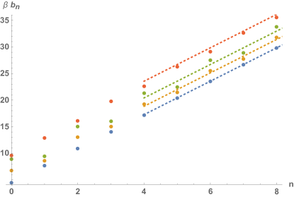
Figure 1: Lanczos coefficients $b_{n}$ for free massless scalar $\phi$ in $d=4$ ($\Delta=1$, blue), $d=5$ ($\Delta=3/2$, orange), $d=6$ ($\Delta=2$, green) dimensions, and for the composite operator $\phi^{2}$ in $d=5$ dimensions ($\Delta=3$, red); dashed lines of the appropriate color show asymptotic behavior of $b_{n}$ as given by (23).

For (15) with general $\Delta$ explicit expression for Lanczos coefficients is not known. In the special case of $d=4$, $C_{0}$ reduces to (14) with $\Delta=1$, and the rest applies. For $d=6$, $\Delta=2$, and Lanczos coefficients can be evaluated using connection to integrable Toda hierarchy Dymarsky and Gorsky (2020), yielding (see Supplemental Material)

$$b_{n}^{2} = \left({\pi/\beta}\right)^{2}(n+2)(n+3){g_{n-1}g_{n+1}\over g_{n}^{2}},$$ (16)

$$g_{n} = H_{n+2}+(-1)^{n+1}\Phi(-1,1,3+n)+\ln(2).$$

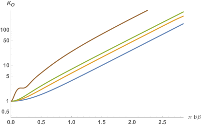
Figure 2: Krylov complexity $K_{\mathcal{O}}$ shown in logarithmic scale for free scalar in $d=4$ (blue), $d=5$ (orange), $d=6$ (green) dimensions and for Generalized Free Field with $\Delta=10$ (brown). Blue curve is known analytically, $\ln(1+2\sinh^{2}(\pi t/\beta))$. All four curves exhibit an apparent linear growth of $\ln K_{\mathcal{O}}\propto 2\pi t/\beta$ at late times.

Here $H_{n}$ is the harmonic number and $\Phi$ is Lerch transcendent. In this case $b_{n}^{2}$ demonstrate ``staggering'' or ``dimerization'' – the sequences of $b_{n}^{2}$ for even and odd $n$ can be combined into two families, each approximately described by smooth functions $b_{n}=h_{n}+(-1)^{n}\tilde{h}_{n}$, where $h_{n}\approx(\pi/2\tau^{*})n+o(n)$ for $n\gg 1$. This is shown in Fig. 1. Such a behavior was analyzed in Yates et al. (2020a, b), where it was shown that for smooth functions $h_{n},\tilde{h}_{n}$ in the large $n$ region ``Schr$\ddot{\rm{o}}$dinger equation'' (6) reduces to continuous Dirac equation with the space-dependent mass. In the case when asymptotically $\tilde{h}_{n}\rightarrow 0$, mass eventually approaches zero for large $x$, describing propagation of a quantum ``particle'' with the speed of light $x(t)\sim t$ with respect to an auxiliary spatial continuous coordinate $x$ which is related to $n$ via Yates et al. (2020b)

$$n\propto(e^{(2\pi/\beta)x}-1).$$ (17)

From this follows that for late times Krylov complexity will grow exponentially

$$K_{\mathcal{O}}(t)\approx e^{2\pi/\beta(t-t_{0})}$$ (18)

where $t_{0}$ is the characteristic time ``quantum particle'' described by $\varphi_{n}(t)$ will spend near the edge of the Krylov space $n\sim O(1)$. From the analytic expression for $K_{\mathcal{O}}$ in case of 2d CFTs we conclude that $t_{0}$ is growing negative for large $\Delta$, $t_{0}\sim-\ln\Delta$. The only scenario to avoid exponential growth of $K_{\mathcal{O}}$ with $t$ is for $\varphi_{n}(t)$ to be localized near the edge $n\sim O(1)$, which would presumably require erratic behavior of $b_{n}$ for small $n$.

Numerical simulation of $K_{\mathcal{O}}$ for massless scalar in $d=6$ shown in Fig. 2 confirms exponential behavior (18) with $t_{0}$ of order one. Thus, despite ``staggering'' Krylov complexity for free massless scalar in $d=6$ behaves qualitatively similar to $d=4$ case.

Next we numerically plot Lanczos coefficients for free scalar in $d=5$ with $\Delta=3/2$, see Fig. 1. Similarly to $d=6$, $b_{n}$'s exhibit staggering, which does not affect asymptotic exponential behavior of $K_{\mathcal{O}}$, see Fig. 2.

To analyze general case (15) with $\Delta\gg 1$ we can approximate $C_{0}$ with an exponential precision by

$$C_{0}\propto{1\over(\beta+2\tau)^{2\Delta}}+{1\over(\beta-2\tau)^{2\Delta}}.$$ (19)

By employing $1/\Delta$ expansion we find for small $n$

$$\beta^{2}b_{n}^{2}=\left\{\begin{array}[]{lc}16\Delta^{2}+8(1+3n)\Delta+{19n^{2}}/{2}+7n+O(n^{3})/\Delta+\dots&{\rm for}\ n\ {\rm even},\\ 16(1+n)\Delta+2(n+1)(5n+1)+O(n^{3})/\Delta+\dots&{\rm for}\ n\ {\rm odd}.\end{array}\right.$$ (22)

Thus, staggering grows with $\Delta$, but $n$ dependence of $b_{n}$ for odd and even $n$ remain smooth.

For large $n$ pole structure of $C_{0}$ suggests, see Supplemental Material,

$$\beta\,b_{n}\approx\pi(n+\Delta+1/2).$$ (23)

These approximations accurately describe $b_{n}$ for small and large $n$ correspondingly, as is shown in the left panel of Fig. 3. Numerical simulation of $K_{\mathcal{O}}(t)$ for $\Delta=10$ shown in Fig. 2 confirms exponential behavior with $\lambda_{K}=2\pi/\beta$ and $t_{0}$ of order $-\ln\Delta$. In other words staggering, exhibited by $b_{n}$ in case o free scalar field, which grows with $\Delta$, is not affecting dynamics at late times – $K_{\mathcal{O}}$ grows exponentially with the exponent $\lambda_{K}=2\pi/\beta$, although dynamics at early times becomes more complicated.

Finally, we discuss composite operators ${\mathcal{O}}^{m}$ for some integer $m$. By Wick theorem Wightman function simply becomes $C_{0}\rightarrow C_{0}^{m}$ with an unimportant overall coefficient. In the case of 2d CFT or free massless scalar in $d=4$ we again obtain $C_{0}$ of the form (14). In other cases Lanczos coefficients should be calculated numerically. We plot $b_{n}$ for ${\mathcal{O}}=\phi^{2}$ in free massless scalar theory in $d=5$ in Fig. 1.

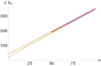
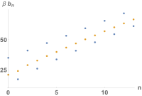
Figure 3: Left panel. Lanczos coefficients $b_{n}$ for Generalized Free Field (15) with $\Delta=10$ (blue) vs approximation for small $n$ (22) (orange) and asymptotic behavior for large $n$ (23) (red line). Right panel. Lanczos coefficients $b_{n}$ for Generalized Free Field (15) of dimension $\Delta=8.5$ (blue) and for holographic operator $O=\int d^{3}x\,{\mathcal{O}}$ of effective dimension $\Delta=8.5$, while ${\mathcal{O}}$ has dimension $\Delta=10$ (orange). The same effective dimension means both sequences have the same asymptotic behavior $b_{n}\approx\pi(n+9)$.

iii) In case of free fermions in $d$ dimensions,

$$C_{\psi}(\tau) = r_{d}\left(\zeta\big{(}2\Delta,{1\over 4}-{\tau\over 2\beta}\big{)}+\zeta\big{(}2\Delta,{1\over 4}+{\tau\over 2\beta}\big{)}\right.$$ (24)

$$- \left.\zeta\big{(}2\Delta,{3\over 4}-{\tau\over 2\beta}\big{)}-\zeta\big{(}2\Delta,{3\over 4}+{\tau\over 2\beta}\big{)}\right),$$

where dimension of free fermion is $\Delta=(d-1)/2$. We notice that Lanczos coefficients for free fermion in dimension $d$ are very close to those for the free boson of the same conformal dimension $\Delta$, i.e. in dimension $d+1$. The same applies for $b_{n}$ for the composite operators $\bar{\psi}\psi$ and $\phi^{2}$. Corresponding comparison is delegated to Supplemental Material.

iv) In case of holographic CFT thermal two-point function can be calculated by solving wave equation in the bulk Festuccia and Liu (2006, 2009). We perform this numerically in Supplemental Material to find that $b_{n}$ smoothly depend on $n$. This is shown in the right panel of Fig. 3 where we superimposed $b_{n}$ for the holographic model with Lanczos coefficients for the Generalized Free Field of the same effective dimension, determined by the singularity of $C_{0}$ near $\tau\rightarrow\beta/2$. Smooth behavior perfectly matches the expectation that for holographic theories exhibiting maximal chaos, $\lambda=2\pi/\beta$, growth of Krylov complexity also must be governed by the same exponent.

Besides Krylov complexity we numerically plot growth of Krylov entropy (8) for several different models, shown in Fig. 4. In all cases it exhibits linear behavior for late $t$, confirming scrambling of ${\mathcal{O}}$ in Krylov space. We conclude that only early time dynamics is sensitive to pecularities of the model, while at late times dynamics in Krylov space exhibits remarkable universality.

Conclusions. In this paper we studied Lanczos coefficients and operator growth in Krylov space for local operators in various CFT models. For some models $b_{n}$ were calculated analytically, while for others we had to resort to numerical analysis. We also found asymptotic behavior of $b_{n}$ for large $n$ (23). One of the main goals was to study if Krylov complexity is sensitive to the underlying chaos. A general argument presented in the introduction dictates that so far asymptotic behavior of $b_{n}$ as a function of $n$ is sufficiently smooth, Lanczos coefficients exhibit universal operator growth hypothesis (12) and Krylov complexity grows exponentially (18). The only possible caveat is the possibility that for large $n$ different subsequences of $b_{n}$ would have different asymptotic, for example $b_{n}$ for even and odd $n$ would grow as $n^{a}$ with different $a_{\rm even}\neq a_{odd}$. Another hypothetical possibility, which will not affect (12) but may affect (18), is that erratic behavior of $b_{n}$ for small $n$ will cause approximate or complete localization of the operator ``wave-function'' $\varphi_{n}$, leading to large or infinite $t_{0}$. We did not see any behavior of this sort in any model we considered, including arbitrary 2d CFTs, free bosons and fermions, composite operators, generalized free field of arbitrary dimension, and a holographic model in $d=4$. On the contrary we observed linear growth of $b_{n}$ at large $n$ in full agreement with (23) and exponential growth of Krylov complexity with $\lambda_{K}=2\pi/\beta$. In other words for considered models universal operator growth hypothesis of Parker et al. (2019) trivially holds, and the conjectural bound (1) on of OTOC at finite temperature in terms of growth of Krylov complexity reduces to MSS bound Maldacena et al. (2016). At the same time exponential growth of $K_{\mathcal{O}}$ is not a signature of chaos as it grows with the same exponent $\lambda_{K}=2\pi/\beta$ for maximally chaotic holographic CFTs as well as for rational 2d CFTs and free field theories, for which Lypanunov exponent may not be even properly defined Caputa et al. (2016); Fan (2018); Kudler-Flam et al. (2020). It would be interesting to extend our analysis for massive an interacting models, especially those exhibiting non-maximal chaos Stanford (2016); Murugan et al. (2017); Steinberg and Swingle (2019); Mezei and Sárosi (2020). Nevertheless since a continuous deformation can not change asymptotic behavior of $b_{n}$ we provisionally conclude our results will remain valid in the case of general interacting quantum field theory.

It is also instructive to compare behavior of Krylov complexity with various notions of circuit and holographic complexities. While the latter are defined for states and the former is a measure of operator growth, an analysis of Barbón et al. (2019); Jian et al. (2020); Rabinovici et al. (2020) in the context of SYK-type models revealed some qualitative similarities. In this spirit we notice that $K_{\mathcal{O}}$ exhibits essentially the same behavior for both free and holographic theories, similarly to complexity action proposal, as discussed in Jefferson and Myers (2017); Chapman et al. (2018). There are also bulk complexity proposals specific for conformal theories Caputa et al. (2017); Caputa and Magan (2019), which exhibit robust universality due to extended symmetry. To complete the comparison, it would be important to go beyond thermodynamic limit by placing CFT on a compact background, e.g. ${\mathbb{S}}^{d-1}\times\mathbb{R}$. In this case one may hope to study qualitative behavior of $K_{\mathcal{O}}$ beyond scrambling time $t\sim\ln S$, when the exponential complexity growth should become linear.

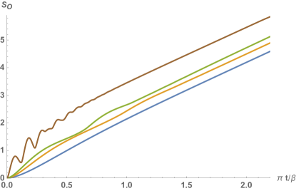
Figure 4: K-entropy $S_{\mathcal{O}}$ shown in logarithmic scale for free scalar in $d=4$ (blue), $d=5$ (orange), $d=6$ (green) dimensions and for Generalized Free Field with $\Delta=10$ (brown). All four curves exhibit an apparent linear growth at late times.

I Supplemental Material

I.1 Lanczos coefficients from the thermal 2pt function

Recursion method is closely related to integrable Toda chain Dymarsky and Gorsky (2020). In particular thermal 2pt function $C_{0}(\tau)$ should be understood as the tau-function of Toda hierarchy, $\tau_{0}\equiv C_{0}$. Other tau-functions $\tau_{n}$ are related to $C_{0}$ as follows. One introduces $(n+1)\times(n+1)$, $n\geq 0$, Hankel matrix of derivatives

$${\mathcal{M}}^{(n)}_{ij}=C_{0}^{(i+j)}(\tau),$$ (25)

where $C_{0}^{(k)}(\tau)$ stands for $k$-th derivative of $C_{0}$. Then

$$\tau_{n}(\tau)={\rm det}\,{\mathcal{M}}^{(n)}.$$ (26)

Tau functions automatically satisfy Hirota bilinear relation

$$\tau_{n}\ddot{\tau}_{n}-\dot{\tau_{n}}^{2}=\tau_{n+1}\tau_{n-1},\quad\tau_{-1}\equiv 1.$$ (27)

At this point we can introduce $q_{n}$ via $\tau_{n}={\rm exp}(\sum_{0\leq k\leq n}q_{n})$, such that $C_{0}(\tau)=e^{q_{0}(\tau)}$. Functions $q_{n}$ satisfy Toda chain equations of motion. Lanczos coefficients are

$$b_{n}^{2}=e^{q_{n+1}-q_{n}}={\tau_{n+1}\tau_{n-1}\over\tau_{n}^{2}}.$$ (28)

Defined this way $b_{n}^{2}$ are functions of $\tau$. To evaluate Lanczos coefficients from (3) we need to take $\tau=0$ in (28). This prescription is equivalent to evaluation of $b_{n}^{2}$ from the moments of $f^{2}(\omega)$ (10) described in Parker et al. (2019).

There is an explicit family of solutions with the asymptotic behavior $b_{n}^{2}\propto n^{2}$ Dymarsky and Gorsky (2020)

$$\tau_{n}(\tau) = {G(n+2)G(n+1+2\Delta)\over G(2\Delta)\Gamma(2\Delta)^{n+1}}{(\pi/\beta)^{n(n+1)}\over\cos(\pi\tau/\beta)^{(n+2\Delta)(n+1)}},$$

$$q_{n}(\tau) = 2n\ln(\pi/\beta)-(2n+2\Delta)\ln(\beta\cos(\pi\tau/\beta))+$$

$$\ln(n!\Gamma(n+2\Delta)),$$ (29)

$$a_{n}(\tau) = (2n+2\Delta)(\pi/\beta)\tan(\pi\tau/\beta),$$

$$b^{2}_{n}(\tau) = {(n+2\Delta)(n+1)(\pi/\beta)^{2}\over\cos^{2}(\pi\tau/\beta)},$$

where $G(x)$ is the Barnes gamma function. This is the solution which appears in the context of $C_{0}$ for the 2d CFTs (14).

I.2 Free massless scalar in $d$ dimensions

For convenience we introduce $\tilde{\tau}=\tau/\beta$. Thermal 2pt function in coordinate space is given by an integral of Matsubara propagator,

$$C_{\phi}(\tilde{\tau},d)={\beta^{2-d}\over(4\pi)^{d-1\over 2}\Gamma\big{(}{d-1\over 2}\big{)}}\int_{0}^{\infty}dy\,y^{d-3}{\cosh(y\tilde{\tau})\over\sinh\big{(}{y\over 2}\big{)}}.$$

The integral over $y$ can be evaluated yielding (15) with $2\Delta=d-2$ and

$$c_{d}=\beta^{2-d}{\Gamma\big{(}{d-2\over 2}\big{)}\over 4\pi^{d\over 2}}.$$ (30)

Numerically Lanczos coefficients for (15) can be evaluated from (26,28) using

$$C_{\phi}^{(2n)}(0)=c_{d}{2(2^{2\Delta+2n}-1)\beta^{-2n}\over\Gamma\big{(}2\Delta\big{)}}\Gamma(2\Delta+2n)\zeta(2\Delta+2n).$$

Up to an overall coefficient for $d=4$ (15) reduces to (14) with $\Delta=1$. It follows from the integral representation above that for integer $d$

$$C_{\phi}(\tilde{\tau},d)\propto{d^{2}\over d\tilde{\tau}^{2}}C_{\phi}(\tilde{\tau},d-2),$$ (32)

and therefore for $d=6$

$$C_{0}(\tau)\propto{d^{2}\over d\tau^{2}}{1\over\cos^{2}(\pi\tau/\beta)}.$$ (33)

To find $b_{n}^{2}$ we look for the tau-functions of the form

$$\tau_{n} = {(\pi/\beta)^{\alpha_{n}}p_{n}(\cos^{2}(\pi\tau/\beta))\over\cos(\pi\tau/\beta)^{a_{n}}},\quad n\geq 1,$$ (34)

$$a_{n} = (n+a)(n+1),\qquad\alpha_{n}=(n+\alpha)(n+1),$$

where $p_{n}(y)$ is a polynomial of degree $n+1$ and $p_{-1}=1$ such that $\tau_{-1}=1$. Then Hirota equations (27) become iterative equations for the polynomials

$$p_{n+1}={a_{n}p_{n}^{2}-4(1-y)y^{2}(p_{n}^{\prime})^{2}+2yp_{n}((1-2y)p_{n}^{\prime}+2(1-y)yp_{n}^{\prime\prime})\over p_{n-1}}.$$ (35)

To match with (33) we take $a=4$, $\alpha=2$ (this value is in fact arbitrary) and $p_{0}=1-2y/3$. Then

$$p_{n}(y)=\prod_{k=0}^{n-1}a_{k}^{n-k}\sum_{k=0}^{n+1}{(-4)^{k}\over(1+k)^{2}}{\Gamma(2+n)\Gamma(4+n+k)y^{k}\over\Gamma(4+n)\Gamma(2+2k)\Gamma(2+n-k)}.$$

This can be evaluated for $y=1$ which corresponds to $\tau=0$,

$$p_{n}(1)={H_{n+2}+\ln(2)+(-1)^{n+1}\Phi(-1,1,n+3)\over(n+2)(n+3)},$$

where $H_{n}=\sum_{k=1}^{n}k^{-1}$ is the harmonic number and $\Phi(z,s,\alpha)=\sum_{k=0}^{\infty}z^{k}/(k+\alpha)^{s}$ is the Lerch transcendent. From here we obtain (16).

The same logic can be applied to $d=8$, in which case $a=6$, and $p_{0}=1-y+2y^{2}/15$. Iterative relation (35) gives

$$p_{n}(y)=\prod_{k=0}^{n-1}a_{k}^{n-k}\left(1-{(n+1)(n+6)\over 6}y+O(y^{2})\right),$$

but we were not able to find closed form analytic expression.

I.3 Pole structure of $C_{0}$ controls asymptote of $b_{n}$

Under the assumption that the $n$-dependence of $b_{n}$ is smooth, at least for large $n\gg 1$, the asymptote of $b_{n}$ is controlled by the poles of $C_{0}$, or equivalently high frequency behavior of $f^{2}(\omega)$. For an operator of dimension $\Delta$ CFT correlator $C_{0}(\tau)$ would have a pole singularity $\propto(\tau-\tau^{*})^{-2\Delta}$ where $\tau^{*}=\beta/2$, implying asymptotic behavior

$$f^{2}(\omega)\propto e^{-\omega\tau^{*}}\omega^{2\Delta-1}$$ (36)

for large $\omega$. Using saddle point approximation we can estimate the moments

$$M_{2k}\equiv{\int_{\-\infty}^{\infty}d\omega f^{2}(\omega)\omega^{2k}\over\int_{\-\infty}^{\infty}d\omega f^{2}(\omega)}\approx{\left({2\tilde{k}\over e\tau^{*}}\right)^{2\tilde{k}}\over\left({2\Delta-1\over e\tau^{*}}\right)^{2\Delta-1}},$$ (37)

where $\tilde{k}=k+\Delta-1/2$. Strictly speaking for validity we need to require $\Delta\rightarrow\infty$. In the case when $\Delta$ is of order one the expression above is valid only in the sense of $k$-dependence in the limit of large $k$. Assuming smooth $k$-dependence of $b_{k}$ we will approximate it by

$$\beta\,b_{k}\approx{\mathfrak{a}}\,k+{\mathfrak{b}},\quad k\gg 1.$$ (38)

It is tempting to rewrite it as $\beta\,b_{k}={\mathfrak{a}}\,\tilde{k}$, and identify ${\mathfrak{b}/\mathfrak{a}}$ with $\Delta-1/2$. To justify that we will use the formalism of integral over Dyck paths which evaluates $M_{2k}$ in terms of $b_{n}$'s developed in Avdoshkin and Dymarsky (2020). At the level of quasiclassical approximation, which gives leading contribution in the limit of large $k$, the moments are given by

$$M_{2k}\approx e^{S},$$ (39)

where $S$ is the on-shell value of action

$$S[f(t)]=2k\int_{0}^{1}dt\left(-p\ln p-(1-p)\ln(1-p)+b(2k{\mathfrak{f}})\right),$$

(40)

where $p\equiv(1+{\mathfrak{f}}^{\prime})/2$, Lanczos coefficients $b_{n}$ are described by the smooth function $b(n)$ and ${\mathfrak{f}}(t)$ satisfies boundary conditions $f(0)=f(1)=0$. For $b(2k{\mathfrak{f}})=2k{\mathfrak{f}}{\mathfrak{a}}+{\mathfrak{b}}$ equation of motion reads

$${{\mathfrak{f}}^{\prime\prime}\over({\mathfrak{f}}^{\prime})^{2}-1}={2k\mathfrak{a}\over 2k\mathfrak{a}{\mathfrak{f}}+\mathfrak{b}}$$ (41)

with the solution

$${\mathfrak{f}}(t)={\sin((\pi-2r)t+r)\over(\pi-2r)}-{\mathfrak{b}\over 2k\mathfrak{a}},$$ (42)

where $r$ is defined from the equation

$${\mathfrak{b}\over 2k\mathfrak{a}}={\sin(r)\over\pi-2r}.$$ (43)

When $k$ goes to infinity this gives the asymptote $r\approx{\mathfrak{b}\pi/2k\mathfrak{a}}$. Plugging the solution (42) back into action (40) yields

$$S=2k\ln\left({4k\mathfrak{a}\over e(\pi-2r)}\right)+2{\mathfrak{b}\over\mathfrak{a}}\ln\cot(r/2).$$ (44)

Taking large $k$ limit we finally arrive at

$$M_{2k}\approx\left({4k\mathfrak{a}\over e\pi}\right)^{2k}e^{2\mathfrak{b}\over\mathfrak{a}}\left({4k\mathfrak{a}\over e\mathfrak{b}}\right)^{2\mathfrak{b}\over\mathfrak{a}}.$$ (45)

Comparing with (37) $k$-dependence we first obtain the result well-appreciated in the literature,

$$\mathfrak{a}={\pi\over 2\tau^{*}},$$ (46)

and then also

$${\mathfrak{b}\over\mathfrak{a}}=\Delta-1/2.$$ (47)

In this subsection we used the formalism of Avdoshkin and Dymarsky (2020) which numerates $b_{n}$ starting from $n=1$. In the main text index $n$ starts from zero, yielding a shift by one in (23).

I.4 Free massless fermion in $d$ dimensions

Integration over the Matsubara propagator yields (24) with

$$r_{d}=\beta^{1-d}{\Gamma\big{(}{d\over 2}\big{)}\over(4\pi)^{d\over 2}}.$$ (48)

It is valid only for $-1/2<\tau/\beta<1/2$ and should be extended by antiperiodicity

$$C_{\psi}(\tau+\beta)=-C_{\psi}(\tau)$$ (49)

beyond that. To evaluate $b_{n}^{2}$ numerically it is helpful to know closed-form expression for the $2n$-th derivative

$$C_{\psi}^{(2n)} = r_{d}{\Gamma(2\Delta+2n)\over 2^{2n-1}\Gamma(2\Delta)}\big{(}\zeta\big{(}2\Delta+2n,{1\over 4}\big{)}-\zeta\big{(}2\Delta+2n,{3\over 4}\big{)}\big{)}.$$

As is pointed out in the main text resulting Lanczos coefficients are numerically very close to those for free scalar of the same conformal dimension $\Delta$. The same applies for composite operators $\bar{\psi}\psi$ and $\phi^{2}$. We illustrate that by the plot in Fig. 5.

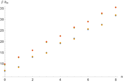
Figure 5: Lanczos coefficients for free scalar (15) in $d=5$ dimensions (blue) and free fermion (24) in $d=4$ dimensions (orange) – in both cases $\Delta=3/2$ and $b_{n}$ are very close to each other and overlap in the plot. Also, Lanczos coefficients for composite operator $\phi^{2}$ in $d=5$ dimensions (green) and composite operator $\bar{\psi}\psi$ in $d=4$ (red) – in both cases $\Delta=3$ and $b_{n}$ are again very close to each other and overlap.

I.5 Holographic thermal 2pt function

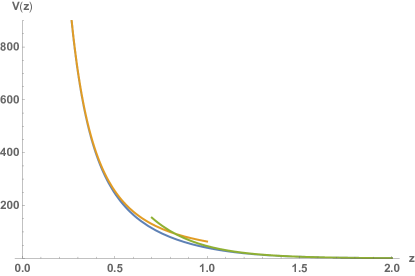
Figure 6: Effective potential $V(z)$ (54) for $d=4,\nu=8$ (blue) vs asymptotic expressions (56) (orange) and (57) (green).

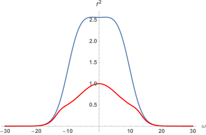
Figure 7: Power spectrum $f^{2}$ given by (60) for $d=4,\nu=8$ calculated using numerical integration from $z_{1}$ to $z_{2}$ (blue) and crude approximation by gluing $\psi_{1}$ and $\psi_{2}$ at $z=z^{*}$ (red). Both expression are multiplied by the same overall coefficient such that in the crude approximation case $f^{2}(0)=1$.

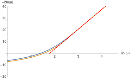
Figure 8: Plot of $-2\ln|a|$ vs $\ln\omega$ calculated using numerical integration from $z_{1}$ to $z_{2}$ (blue) and crude approximation by gluing $\psi_{1}$ and $\psi_{2}$ at $z=z^{*}$ (orange) vs linear fit describing large $\omega$ behavior (red dashed line).

CFT on $\mathbb{R}^{1,d}$ at finite temperature $\beta$ is holographically described by a black brane background. To evaluate Wightman 2pt function $C_{0}(\tau)$ one needs to solve the wave-equation for a scalar field in the bulk dual to an operator ${\mathcal{O}}$ of dimension $\Delta$. For simplicity we will consider ${\mathcal{O}}$ at zero spatial momentum, i.e. our operator in question is

$$O(t)={1\over\sqrt{\rm Volume}}\int d^{d-1}x\,{\mathcal{O}}(t,x),$$ (51)

where overall normalization is chosen such that two-point function of $O$ is finite. Then the power spectrum $f^{2}(\omega)$ associated with

$$C_{0}(\tau) = \operatorname{Tr}(e^{-(\beta-\tau)H/2}Oe^{-(\beta+\tau)}O)=$$ (52)

$$\int d^{d-1}x\,\langle{\mathcal{O}}(i(\tau+\beta/2,\vec{x}){\mathcal{O}}(0,\vec{0})\rangle_{\beta},$$

is given by the following procedure Festuccia and Liu (2006, 2009). One introduces tortoise coordinate in the bulk

$$z=\int_{r}^{\infty}{dr\over{\mathfrak{f}}},\qquad{\mathfrak{f}}=r^{2}-{1\over r^{d-2}},$$ (53)

and an effective potential

$$V(z)={\mathfrak{f}}(r)\left(\nu^{2}-1/4+{(d-1)^{2}\over 4r^{d}}\right),$$ (54)

$$\Delta=d/2+\nu.$$

The scalar in the bulk dual to ${\mathcal{O}}$ satisfies ``Schrodinger'' equation

$$-{d^{2}\psi\over dz^{2}}+V\psi=\omega^{2}\psi,\quad 0\leq z<\infty.$$ (55)

Near $z\rightarrow 0$ the potential behaves as

$$V(z)\approx{\nu^{2}-1/4\over z^{2}},$$ (56)

and at large $z$

$$V(z)\approx 8\left(\nu^{2}+2\right)e^{\frac{\pi}{2}-4z},$$ (57)

where we restricted to $d=4$. The boundary behavior of $\psi$ is therefore

$$\psi(z) \approx z^{\nu+1/2},\quad z\rightarrow 0,$$ (58)

$$\psi(z) \approx a\,e^{-i\omega z}+\bar{a}\,e^{i\omega z},\quad z\rightarrow\infty,$$ (59)

where $a$ is a complex $\omega$-dependent constant. The power spectrum of $C_{0}$ is then given by

$$f^{2}(\omega)\propto{|a|^{-2}\over\omega\sinh(\beta\omega/2)},$$ (60)

where temperature is fixed to be $\beta=4\pi/d$.

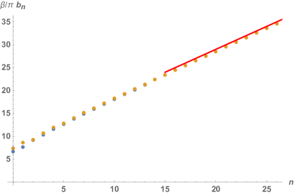
Figure 9: ``Holographic'' Lanczos coefficients $b_{n}$ for $0\leq n\leq 13$ evaluated using numerical integration from $z_{1}$ to $z_{2}$ (blue), $b_{n}$ evaluated using gluing $\psi_{1}$ and $\psi_{2}$ at $z=z^{*}$ (orange) and asymptotic behavior given by (23), $(\beta/\pi)b_{n}\approx n+\Delta-1$ (red line).

To obtain $f^{2}(\omega)$ numerically one needs to solve (55) with the boundary conditions (58,59). In practice the asymptotic approximations (56,57) accurately describe $V(z)$ everywhere outside of a small region of $z\sim 1$, as is shown in Fig. 6 for $d=4$ and $\nu=8$ which corresponds to $\Delta=10$. ``Schrodinger'' equation (55) with the approximate potential (56) or (57) can be solved analytically

$$\psi_{1}=\sqrt{z}\left(\frac{2}{\omega}\right)^{\nu}\Gamma(\nu+1)J_{\nu}(z\omega),$$ (61)

for small $z$ and

$$\psi_{2}=a\,\Gamma\left(\frac{i\omega}{2}+1\right)I_{i\frac{\omega}{2}}\left(e^{\pi/4}\sqrt{2(\nu^{2}+2)}\,e^{-2z}\right)+{\rm c.c.}$$

for large $z$. A crude approximation would be to neglect the region around $z\sim 1$ where asymptotic expressions (56) and (57) are less accurate and simply glue $\psi_{1}$ and $\psi_{2}$ at some intermediate point $z=z^{*}$ by continuity (and continuity of $\psi^{\prime}$). We choose $z^{*}\approx 0.8251$ such that $V_{1}(z^{*})=V_{2}(z^{*})$. A more accurate approach would be to use $\psi_{1}$ for $z\leq z_{1}$ and $\psi_{2}$ for $z\geq z_{2}$, while integrating (55) numerically from $z_{1}$ to $z_{2}$. We choose $z_{1}=0.2$ and $z_{2}=3$. Resulting profiles of $f^{2}(\omega)$ differ, as shown in Fig. 7, but asymptotic behavior at large $\omega$ is the same. We confirm that by plotting $|a|^{-2}$ in logarithmic scale superimposed with a linear fit in Fig. 8. The slope of the linear fit is $16.99$ which perfectly matches the expected asymptotic behavior of $f^{2}$ (36) after we take into account that (52) in the limit $\tau\rightarrow\beta/2$ has a singularity $C_{0}\propto(\tau-\beta/2)^{2\Delta-3}$.

With this we proceed to evaluate the moments (37) and Lanczos coefficients. The latter are shown in Fig. 9 for both approximations superimposed with the asymptotic fit (23).

References

- D'Alessio et al. (2016) Luca D'Alessio, Yariv Kafri, Anatoli Polkovnikov, and Marcos Rigol, ``From quantum chaos and eigenstate thermalization to statistical mechanics and thermodynamics,'' Advances in Physics 65, 239–362 (2016).
- Maldacena et al. (2016) Juan Maldacena, Stephen H Shenker, and Douglas Stanford, ``A bound on chaos,'' Journal of High Energy Physics 2016, 1–17 (2016).
- Parker et al. (2019) Daniel E Parker, Xiangyu Cao, Alexander Avdoshkin, Thomas Scaffidi, and Ehud Altman, ``A universal operator growth hypothesis,'' Physical Review X 9, 041017 (2019).
- Maldacena and Stanford (2016) Juan Maldacena and Douglas Stanford, ``Remarks on the sachdev-ye-kitaev model,'' Phys. Rev. D 94, 106002 (2016).
- Rosenhaus (2019) Vladimir Rosenhaus, ``An introduction to the syk model,'' Journal of Physics A: Mathematical and Theoretical 52, 323001 (2019).
- Trunin (2020) Dmitrii A Trunin, ``Pedagogical introduction to syk model and 2d dilaton gravity,'' arXiv preprint arXiv:2002.12187 (2020).
- Roberts et al. (2015) Daniel A Roberts, Douglas Stanford, and Leonard Susskind, ``Localized shocks,'' Journal of High Energy Physics 2015, 51 (2015).
- Hartman et al. (2017) Thomas Hartman, Sean A Hartnoll, and Raghu Mahajan, ``Upper bound on diffusivity,'' Physical review letters 119, 141601 (2017).
- Murthy and Srednicki (2019) Chaitanya Murthy and Mark Srednicki, ``Bounds on chaos from the eigenstate thermalization hypothesis,'' Physical review letters 123, 230606 (2019).
- Barbón et al. (2019) JLF Barbón, E Rabinovici, R Shir, and R Sinha, ``On the evolution of operator complexity beyond scrambling,'' Journal of High Energy Physics 2019, 1–25 (2019).
- Jian et al. (2020) Shao-Kai Jian, Brian Swingle, and Zhuo-Yu Xian, ``Complexity growth of operators in the syk model and in jt gravity,'' arXiv preprint arXiv:2008.12274 (2020).
- Rabinovici et al. (2020) E Rabinovici, A Sánchez-Garrido, R Shir, and J Sonner, ``Operator complexity: a journey to the edge of krylov space,'' arXiv preprint arXiv:2009.01862 (2020).
- Brown et al. (2016) Adam R Brown, Daniel A Roberts, Leonard Susskind, Brian Swingle, and Ying Zhao, ``Holographic complexity equals bulk action?'' Physical review letters 116, 191301 (2016).
- Nunez and Starinets (2003) Alvaro Nunez and Andrei O Starinets, ``Ads/cft correspondence, quasinormal modes, and thermal correlators in n= 4 supersymmetric yang-mills theory,'' Physical Review D 67, 124013 (2003).
- Fidkowski et al. (2004) Lukasz Fidkowski, Veronika Hubeny, Matthew Kleban, and Stephen Shenker, ``The black hole singularity in ads/cft,'' Journal of High Energy Physics 2004, 014 (2004).
- Festuccia and Liu (2006) Guido Festuccia and Hong Liu, ``Excursions beyond the horizon: Black hole singularities in yang-mills theories (i),'' Journal of High Energy Physics 2006, 044 (2006).
- Festuccia and Liu (2009) Guido Festuccia and Hong Liu, ``A bohr-sommerfeld quantization formula for quasinormal frequencies of ads black holes,'' Advanced Science Letters 2, 221–235 (2009).
- Iliesiu et al. (2018) Luca Iliesiu, Murat Koloğlu, Raghu Mahajan, Eric Perlmutter, and David Simmons-Duffin, ``The conformal bootstrap at finite temperature,'' Journal of High Energy Physics 2018, 1–71 (2018).
- Alday et al. (2020) Luis F Alday, Murat Kologlu, and Alexander Zhiboedov, ``Holographic correlators at finite temperature,'' arXiv preprint arXiv:2009.10062 (2020).
- Karlsson et al. (2021) Robin Karlsson, Andrei Parnachev, and Petar Tadić, ``Thermalization in large-n cfts,'' arXiv preprint arXiv:2102.04953 (2021).
- Rodriguez-Gomez and Russo (2021) D Rodriguez-Gomez and JG Russo, ``Correlation functions in finite temperature cft and black hole singularities,'' arXiv preprint arXiv:2102.11891 (2021).
- Dymarsky and Gorsky (2020) Anatoly Dymarsky and Alexander Gorsky, ``Quantum chaos as delocalization in krylov space,'' Physical Review B 102, 085137 (2020).
- Elsayed et al. (2014) Tarek A Elsayed, Benjamin Hess, and Boris V Fine, ``Signatures of chaos in time series generated by many-spin systems at high temperatures,'' Physical Review E 90, 022910 (2014).
- Avdoshkin and Dymarsky (2020) Alexander Avdoshkin and Anatoly Dymarsky, ``Euclidean operator growth and quantum chaos,'' Physical Review Research 2, 043234 (2020).
- Lubinsky (1993) DS Lubinsky, ``An update on orthogonal polynomials and weighted approximation on the real line,'' Acta Applicandae Mathematica 33, 121–164 (1993).
- Basor et al. (2001) Estelle L Basor, Yang Chen, and Harold Widom, ``Determinants of hankel matrices,'' Journal of Functional Analysis 179, 214–234 (2001).
- Yates et al. (2020a) Daniel J Yates, Alexander G Abanov, and Aditi Mitra, ``Lifetime of almost strong edge-mode operators in one-dimensional, interacting, symmetry protected topological phases,'' Physical Review Letters 124, 206803 (2020a).
- Yates et al. (2020b) Daniel J Yates, Alexander G Abanov, and Aditi Mitra, ``Dynamics of almost strong edge modes in spin chains away from integrability,'' Physical Review B 102, 195419 (2020b).
- Caputa et al. (2016) Pawel Caputa, Tokiro Numasawa, and Alvaro Veliz-Osorio, ``Scrambling without chaos in rcft,'' arXiv preprint arXiv:1602.06542 (2016).
- Fan (2018) Ruihua Fan, ``Out-of-time-order correlation functions for unitary minimal models,'' arXiv preprint arXiv:1809.07228 (2018).
- Kudler-Flam et al. (2020) Jonah Kudler-Flam, Laimei Nie, and Shinsei Ryu, ``Conformal field theory and the web of quantum chaos diagnostics,'' Journal of High Energy Physics 2020, 1–33 (2020).
- Stanford (2016) Douglas Stanford, ``Many-body chaos at weak coupling,'' Journal of High Energy Physics 2016, 1–18 (2016).
- Murugan et al. (2017) Jeff Murugan, Douglas Stanford, and Edward Witten, ``More on supersymmetric and 2d analogs of the syk model,'' Journal of High Energy Physics 2017, 1–99 (2017).
- Steinberg and Swingle (2019) Julia Steinberg and Brian Swingle, ``Thermalization and chaos in qed 3,'' Physical Review D 99, 076007 (2019).
- Mezei and Sárosi (2020) Márk Mezei and Gábor Sárosi, ``Chaos in the butterfly cone,'' Journal of High Energy Physics 2020, 1–34 (2020).
- Jefferson and Myers (2017) Robert A Jefferson and Robert C Myers, ``Circuit complexity in quantum field theory,'' Journal of High Energy Physics 2017, 1–81 (2017).
- Chapman et al. (2018) Shira Chapman, Michal P. Heller, Hugo Marrochio, and Fernando Pastawski, ``Toward a definition of complexity for quantum field theory states,'' Phys. Rev. Lett. 120, 121602 (2018).
- Caputa et al. (2017) Pawel Caputa, Nilay Kundu, Masamichi Miyaji, Tadashi Takayanagi, and Kento Watanabe, ``Liouville action as path-integral complexity: from continuous tensor networks to ads/cft,'' Journal of High Energy Physics 2017, 97 (2017).
- Caputa and Magan (2019) Paweł Caputa and Javier M Magan, ``Quantum computation as gravity,'' Physical review letters 122, 231302 (2019).