A Thesaurus for Common Priors in Gravitational-Wave Astronomy

Abstract

In gravitational-wave data analysis, we regularly work with a host of non-trivial prior probabilities on compact binary masses, redshifts, and spins. We must regularly manipulate these priors, computing the implied priors on a transformed basis of parameters or reweighting posterior samples from one prior to another. Here, I detail some common manipulations, presenting a table of Jacobians with which to transform priors between mass parametrizations, describing the conversion between source- and detector-frame priors, and deriving analytic expressions for priors on the “effective spin” parameters regularly invoked in gravitational-wave astronomy.

I Introduction

Prior probability distributions play an important role in gravitational-wave astronomy. Non-trivial priors on compact binary masses, spins, and redshifts are introduced when measuring the properties of a given system via Bayesian parameter estimation [1, 2, 3, 4]. And farther downstream, hierarchical analysis of the compact binary population relies crucially on being able to write down and “undo” parameter estimation priors to make way for a new population-informed prior that we seek to infer from the data [5, 6, 7, 8, 9, 10, 11, 12].

We not infrequently need to manipulate these priors, determining the implicit prior on some derived quantity, or transforming from one set of priors to another that is more physically justified. Here, I list some formulas to aid in the usage and manipulation of gravitational-wave priors. Many of the expressions below are rather easily obtained but tiring to re-derive every time they’re needed. Others require considerable calculation and/or illuminate critical operations that are frequently mentioned in the literature but rarely presented explicitly.

The contents of this document are organized as follows:

• In Sect. II, I present a table of Jacobians needed to transform probability distributions between different pairs of mass parameters.

• In Sect. III, I illustrate how priors on detector-frame masses and Euclidean distance are converted to priors on redshift and source-frame masses.

• Finally, in Sect. IV, I give analytic expressions translating two common priors on compact binary spins (aligned and isotropic orientations) into their implied priors on the so-called “effective inspiral spin” and “effective precessing spin” parameters.

Although the results in Sect. IV are presented without proof for brevity, I have included the sometimes-lengthy derivations of these results as separate appendices. Also, I have provided a set of python functions that implement the main results of Sect. IV at: https://github.com/tcallister/effective-spin-priors [13].

II Translating Between Mass Parameters

We need only two parameters to uniquely specify the component masses of a compact binary. However, we regularly invoke at least six parameters: the actual component masses $m_{1}$ and $m_{2}$ (with $m_{2}\leq m_{1}$), the total mass $M=m_{1}+m_{2}$, the mass ratio $q=m_{2}/m_{1}$, the symmetric mass ratio $\eta=m_{1}m_{2}/(m_{1}+m_{2})^{2}=q/(1+q)^{2}$, and the chirp mass $\mathcal{M}_{c}=\eta^{3/5}M=m_{1}^{3/5}m_{2}^{3/5}M^{-1/5}$. We often need to transform prior densities defined on one pair of mass variables into the equivalent prior density defined on some other pair. We might, for example, be interested in the prior defined on the two component masses (say, in order to remove said prior during hierarchical modeling) but be given posterior samples whose prior was instead defined on chirp mass and mass ratio.

Table 1: Jacobians $J=\frac{\partial(A,B)}{\partial(C,D)}$ for transforming probability densities from the mass parameter pairs labeling columns to pairs labeling rows. Elements in the empty upper-right corner are found by inverting the inverse Jacobian from the lower-left corner.

		$\left(A,B\right)$
		$(\mathcal{M}_{c},M)$	$(\mathcal{M}_{c},m_{1})$	$(\mathcal{M}_{c},m_{2})$	$(\mathcal{M}_{c},q)$	$(M,m_{1})$	$(M,m_{2})$	$(M,q)$	$(m_{1},m_{2})$	$(m_{1},q)$	$(m_{2},q)$
$(C,D)$	$(\mathcal{M}_{c},M)$	$1$	–	–	–	–	–	–	–	–	–
	$(\mathcal{M}_{c},m_{1})$	$\dfrac{3m_{1}^{2}m_{2}^{2}(m_{1}-m_{2})}{3m_{1}^{3}m_{2}^{2}-\mathcal{M}_{c}^{5}}$	$1$	–	–	–	–	–	–	–	–
	$(\mathcal{M}_{c},m_{2})$	$\dfrac{3m_{1}^{2}m_{2}^{2}(m_{1}-m_{2})}{3m_{1}^{2}m_{2}^{3}-\mathcal{M}_{c}^{5}}$	$\dfrac{\mathcal{M}_{c}^{5}-3m_{1}^{3}m_{2}^{2}}{\mathcal{M}_{c}^{5}-3m_{1}^{2}m_{2}^{3}}$	$1$	–	–	–	–	–	–	–
	$(\mathcal{M}_{c},q)$	$\dfrac{3M(1-q)}{5q(1+q)}$	$\dfrac{\mathcal{M}_{c}(3+2q)}{5q^{8/5}(1+q)^{4/5}}$	$\dfrac{M(2+3q)}{5(1+q)^{2}}$	1	–	–	–	–	–	–
	$(M,m_{1})$	$\dfrac{3\mathcal{M}_{c}(1-q^{2})}{5Mq}$	$\dfrac{3+2q}{5q^{2/5}(1+q)^{6/5}}$	$\dfrac{\mathcal{M}_{c}(2+3q)}{5M}$	$\dfrac{\mathcal{M}_{c}}{m_{1}^{2}}$	$1$	–	–	–	–	–
	$(M,m_{2})$	$\dfrac{3\mathcal{M}_{c}(1-q^{2})}{5Mq}$	$\dfrac{3+2q}{5q^{2/5}(1+q)^{6/5}}$	$\dfrac{\mathcal{M}_{c}(2+3q)}{5M}$	$\dfrac{\mathcal{M}_{c}}{m_{1}^{2}}$	$1$	$1$	–	–	–	–
	$(M,q)$	$\dfrac{3\mathcal{M}_{c}(1-q)}{5q(1+q)}$	$\dfrac{\mathcal{M}_{c}(3+2q)}{5q(1+q)^{2}}$	$\dfrac{\mathcal{M}_{c}(2+3q)}{5(1+q)^{2}}$	$\eta^{3/5}$	$\dfrac{M}{(1+q)^{2}}$	$\dfrac{M}{(1+q)^{2}}$	$1$	–	–	–
	$(m_{1},m_{2})$	$\dfrac{3\mathcal{M}_{c}(1-q^{2})}{5Mq}$	$\dfrac{3+2q}{5q^{2/5}(1+q)^{6/5}}$	$\dfrac{\mathcal{M}_{c}(2+3q)}{5M}$	$\dfrac{\mathcal{M}_{c}}{m_{1}^{2}}$	$1$	$1$	$\dfrac{(1+q)^{2}}{M}$	$1$	–	–
	$(m_{1},q)$	$\dfrac{3\mathcal{M}_{c}(1-q)}{5q}$	$\dfrac{\mathcal{M}_{c}(3+2q)}{5q(1+q)}$	$\dfrac{\mathcal{M}_{c}(2+3q)}{5(1+q)}$	$\eta^{3/5}(1+q)$	$m_{1}$	$m_{1}$	$1+q$	$m_{1}$	$1$	–
	$(m_{2},q)$	$\dfrac{3\mathcal{M}_{c}(1-q)}{5q^{2}}$	$\dfrac{\mathcal{M}_{c}(3+2q)}{5q^{2}(1+q)}$	$\dfrac{\mathcal{M}_{c}(2+3q)}{5q(1+q)}$	$\eta^{3/5}\frac{1+q}{q}$	$\dfrac{m_{2}}{q^{2}}$	$\dfrac{m_{2}}{q^{2}}$	$\dfrac{1+q}{q}$	$\dfrac{m_{2}}{q^{2}}$	$\dfrac{1}{q}$	$1$

In Table 1, I list the Jacobian factors $J=\frac{\partial(A,B)}{\partial(C,D)}$ required to transform between probability densities defined on any combination of $\{\mathcal{M}_{c},M,m_{1},m_{2},q\}$, where column headings denote the pair $(A,B)$ and row headings the target pair $(C,D)$. Jacobians obey the convenient relation $\frac{\partial(A,B)}{\partial(C,D)}=\left(\frac{\partial(C,D)}{\partial(A,B)}\right)^{-1}$, and so any Jacobian in the blank upper-right portion of the table can be obtained by inverting the Jacobian for the inverse transformation in the lower-left portion.

III From the detector frame to the source frame

Another common operation is to translate priors defined on observed detector frame quantities into the implicit priors imposed on source frame parameters. In a Newtonian universe, the gravitational-wave signal received at Earth from a distant source would depend on the source’s distance $D$ and component masses $m_{i}$. Our universe is not Newtonian, but exhibits a non-trivial expansion history governed by general relativity. In this context, observed gravitational-wave signals depend not on source-frame component masses $m_{i}$, but on the detector-frame masses (or “redshifted masses”) $\tilde{m}_{i}=m_{i}(1+z)$, and similarly on the luminosity distance

$$D_{L}(z)=D_{C}(1+z)=(1+z)\int_{0}^{z^{\prime}}\frac{c\,dz^{\prime}}{H(z^{\prime})},$$ (1)

rather than the comoving distance $D_{C}$. In Eq. (1), $c$ is the speed of light and $H(z)$ the Hubble parameter. Note that we are presuming a flat Universe; in the case of non-vanishing curvature Eq. (1) would take a different form (see Eq. 16 of Ref. [14]), modifying the results below.

Parameter estimation codes like lalinference [2] are typically unaware of cosmology; the component masses measured are actually the detector-frame masses (denoted $\tilde{m}_{i}$), and the source distance actually a luminosity distance. Correspondingly, the mass priors are in fact priors $p(\tilde{m}_{i})$ on these detector-frame quantities, which imply some non-trivial joint prior on the source-frame masses and redshift of a particular source. Meanwhile, a seemingly innocuous prior $p(D)\propto D^{2}$ that is uniform in volume is in actuality uniform in “luminosity volume”: $p(D_{L})\propto D_{L}^{2}$.

In hierarchical inference of the source-frame masses and redshifts, a necessary step is the removal of this prior. This, in turn, requires knowing the prior $p(m_{1},m_{2},z)$ implicitly imposed by a detector-frame prior $p(\tilde{m}_{1},\tilde{m}_{2},D_{L})$. Given a prior probability defined on $\{\tilde{m}_{1},\tilde{m}_{2},D_{L}\}$, the corresponding density on $\{m_{1},m_{2},z\}$ is

$$p(m_{1},m_{2},z) =\frac{d^{3}P}{dm_{1}dm_{2}dz}$$ (2)

$$=\frac{d^{3}P}{d\tilde{m}_{1}d\tilde{m}_{2}dD_{L}}\left|\frac{\partial(\tilde{m}_{1},\tilde{m}_{2},D_{L})}{\partial(m_{1},m_{2},z)}\right|$$

$$\propto\Big{(}p(\tilde{m}_{1},\tilde{m}_{2})D_{L}^{2}\Big{)}\begin{vmatrix}1+z&0&m_{1}\\ 0&1+z&m_{2}\\ 0&0&\dfrac{dD_{L}}{dz}\end{vmatrix}$$

$$\propto p(\tilde{m}_{1},\tilde{m}_{2})\left(1+z\right)^{2}D_{L}^{2}(z)\frac{dD_{L}}{dz}.$$

Using the definitions of luminosity and comoving distances from above, we get

$$\boxed{p(m_{1},m_{2},z)\propto p(\tilde{m}_{1},\tilde{m}_{2})\left(1+z\right)^{2}D_{L}^{2}(z)\left[D_{C}(z)+\frac{c(1+z)}{H(z)}\right]}$$ (3)

IV Spin magnitudes, spin components, and effective spins

Priors on the spins of compact binaries are typically written down in terms of the dimensionless spin magnitude $a\in[0,1]$ and tilt angle $t$ relative to the orbital angular momentum. It sometimes important, though, to know the corresponding implicit prior on the actual spin components: the component $s_{z}=a\cos t$ parallel to the orbital angular momentum, and the component $s_{p}=a\sin t$ lying in the orbital plane. We also frequently work in terms of effective spin parameters, including the effective inspiral spin

$$\chi_{\rm eff}=\frac{a_{1}\cos t_{1}+q\,a_{2}\cos t_{2}}{1+q}$$ (4)

quantifying the mass-weighted average spin in the $z$-direction [15, 16], and the effective precessing spin

$$\chi_{p}=\max\Big{[}a_{1}\sin t_{1},\,\left(\frac{3+4q}{4+3q}\right)q\,a_{2}\sin t_{2}\Big{]}.$$ (5)

that roughly corresponds to the degree of in-plane spins [17].

In the following two subsections, I consider two common priors imposed on spin magnitudes and tilts and give the corresponding implicit priors on $s_{z}$, $s_{p}$, $\chi_{\rm eff}$, and $\chi_{p}$. The derivations of these results are at times rather involved, and so are shown separately in Appendices A and B.

IV.1 Uniform & aligned component spin priors

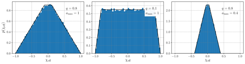
Figure 1: The $\chi_{\rm eff}$ prior distributions constructed via random draws from aligned spin priors under several different values of $q$ and $a_{\rm max}$, compared to the analytic expression in Eq. (7).

Consider a uniform distribution of component spin magnitudes, with directions assumed to be perfectly aligned with a binary’s orbital angular momentum, such that $s_{p}=0$ and

$$p(s_{1,z})=p(s_{2,z})=\frac{1}{2\,a_{\rm max}},$$ (6)

defined on the interval $s_{i,z}\in[-a_{\rm max},a_{\rm max}]$. Priors of this form might be used when performing parameter estimation with various families of “aligned-spin” waveforms, including IMRPhenomD [18, 19] and SEOBNRv4 [20]. Perhaps more importantly, aligned-spin population priors were also used in generating the injection sets [21] employed to measure the Advanced LIGO & Virgo selection function during the O3a observing run [12, 22].

Given a uniform aligned spin prior, the corresponding prior on the effective spin $\chi_{\rm eff}$ is

$$\boxed{p(\chi_{\rm eff}|q)=\begin{cases}0&\Big{(}\chi_{\rm eff}\leq-a_{\rm max}\,\,\mathrm{or}\,\,\chi_{\rm eff}\geq a_{\rm max}\Big{)}\\[10.0pt] \dfrac{(1+q)^{2}\left(a_{\rm max}-\chi_{\rm eff}\right)}{4\,q\,a_{\rm max}^{2}}&\left(\chi_{\rm eff}>\dfrac{1-q}{1+q}\,a_{\rm max},\,\,\chi_{\rm eff}<a_{\rm max}\right)\\[10.0pt] \dfrac{(1+q)^{2}\left(a_{\rm max}+\chi_{\rm eff}\right)}{4\,q\,a_{\rm max}^{2}}&\left(\chi_{\rm eff}<-\dfrac{1-q}{1+q}\,a_{\rm max},\,\,\chi_{\rm eff}>-a_{\rm max}\right)\\[10.0pt] \dfrac{1+q}{2\,a_{\rm max}}&\big{(}{\rm else}\big{)}.\end{cases}}$$ (7)

This expression is derived in Appendix A. Figure 1 compares Eq. (7) to $\chi_{\rm eff}$ prior distributions constructed numerically by randomly drawing pairs of aligned spin values, subject to several different values of $q$ and $a_{\rm max}$. Note that, given its dependence on the mass ratio, Eq. (7) is conditional on $q$. If the marginal mass ratio prior $p(q)$ is known, then the joint prior on $q$ and $\chi_{\rm eff}$ can be expressed via the product $p(\chi_{\rm eff},q)=p(\chi_{\rm eff}|q)\,p(q)$.

IV.2 Uniform & isotropic component spin priors

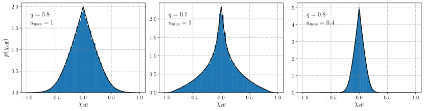
Figure 2: The $\chi_{\rm eff}$ distributions implied by random draws from isotropic spin priors with several different values of $q$ and $a_{\rm max}$, compared to the analytic expression in Eq. (10). Together, these three examples activate every piecewise case in Eq. (10).

Again consider a uniform uniform prior $p(a)=\frac{1}{a_{\rm max}}$ on component spin magnitudes on the interval $0\leq a\leq a_{\rm max}$, but now with an isotropic prior $p(\cos t)=\frac{1}{2}$ on their direction. The corresponding joint prior on the aligned spin component $s_{z}=a\cos t$ and in-plane spin $s_{p}=a\sin t$ is

$$\boxed{p(s_{z},s_{p})=\frac{1}{2a_{\rm max}}\frac{s_{p}}{s_{z}^{2}+s_{p}^{2}}.}$$ (8)

The marginal priors on $s_{z}$ and $s_{p}$ individually are

$$\boxed{\begin{aligned} p(s_{z})&=\frac{1}{2a_{\rm max}}\ln\left(\frac{a_{\rm max}}{|s_{z}|}\right)\\ p(s_{p})&=\frac{1}{a_{\rm max}}\cos^{-1}\left(\frac{s_{p}}{a_{\rm max}}\right).\end{aligned}}$$ (9)

The marginal prior on $\chi_{\rm eff}$ is quite non-trivial to write down, but is most concisely expressed in the form

$$\boxed{p(\chi_{\rm eff}|q)=\begin{cases}\mathrm{Eq.~{}\eqref{eq:p-xeff-0}}&\Big{(}\chi_{\rm eff}=0\Big{)}\\[13.0pt] \mathrm{Eq.~{}\eqref{eq:p-xeff-1}}&\left(\begin{aligned} |\chi_{\rm eff}|<a_{\rm max}\left(\dfrac{1-q}{1+q}\right),\,|\chi_{\rm eff}|<\dfrac{qa_{\rm max}}{1+q}\end{aligned}\right)\\[13.0pt] \mathrm{Eq.~{}\eqref{eq:p-xeff-2}}&\left(|\chi_{\rm eff}|<a_{\rm max}\left(\dfrac{1-q}{1+q}\right),\,|\chi_{\rm eff}|>\dfrac{qa_{\rm max}}{1+q}\right)\\[13.0pt] \mathrm{Eq.~{}\eqref{eq:p-xeff-3}}&\left(|\chi_{\rm eff}|>a_{\rm max}\left(\dfrac{1-q}{1+q}\right),\,|\chi_{\rm eff}|<\dfrac{qa_{\rm max}}{1+q}\right)\\[13.0pt] \mathrm{Eq.~{}\eqref{eq:p-xeff-4}}&\left(|\chi_{\rm eff}|>a_{\rm max}\left(\dfrac{1-q}{1+q}\right),\,|\chi_{\rm eff}|<\dfrac{a_{\rm max}}{1+q},\,|\chi_{\rm eff}|>\dfrac{qa_{\rm max}}{1+q}\right)\\[13.0pt] \mathrm{Eq.~{}\eqref{eq:p-xeff-5}}&\left(|\chi_{\rm eff}|>\dfrac{a_{\rm max}}{1+q},\,|\chi_{\rm eff}|<a_{\rm max}\right)\\[15.0pt] 0&\Big{(}|\chi_{\rm eff}|\geq a_{\rm max}\Big{)}\end{cases}}$$ (10)

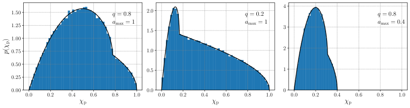
Figure 3: The $\chi_{p}$ distributions implied by random draws from isotropic spin priors with several different values of $q$ and $a_{\rm max}$, compared to the analytic expression in Eq. (11).

The marginal prior on $\chi_{p}$, meanwhile, is given by

$$\boxed{p(\chi_{p}|q)=\mathrm{Eq.~{}\eqref{eq:chip-1}}\,+\,\mathrm{Eq.~{}\eqref{eq:chip-2}}.}$$ (11)

The derivation of Eqs. (8)-(11) is given in Appendix B, which also contains the full expressions referenced here in Eq. (10) and Eq. (11)

Figures 2 and 3 compare these analytic (if daunting) expressions to the $\chi_{\rm eff}$ and $\chi_{p}$ distributions constructed numerically by drawing random spin magnitudes and tilts from a uniform and isotropic prior. The various combinations of $q$ and $a_{\rm max}$ are chosen such that, across the three examples in Fig. 2, we encounter each piecewise case in Eq. (10).

Code that implements Eqs. (10) and (11) is available at the github link in Ref. [13]. Two additional notes concerning the implementation of Eq. (10): First, as mentioned below in Appendix B, Eq. (10) depends on a special function called the “dilogarithm” or “Spence’s function” [23]. Mathematica [24] and scipy [25] adopt different conventions in their implementation of this function. In Appendix B, I follow Mathematica’s convention, such that the quantity I denote $\,{\rm Li}_{2}(z)$ is equivalent to Mathematica’s PolyLog[2,z]. When translated to python, the corresponding quantity is obtained by calling scipy.special.spence(1-z). Second, a very careful reader or user will notice that Eq. (10) is undefined on the boundaries between cases. Rather than consider every possible boundary (of which there are many) as a separate edge case, I instead deal with boundary cases simply by averaging the nearby values $p(\chi_{\rm eff}+\epsilon|q)$ and $p(\chi_{\rm eff}-\epsilon|q)$, for a small offset $\epsilon$. Since $p(\chi_{\rm eff}|q)$ is quite smooth everywhere except the origin, this gives an accurate estimate of the prior at any $\chi_{\rm eff}$ sitting on a boundary between two cases.

APPENDIX A DERIVING $p(\chi_{\rm eff}|q)$ FROM ALIGNED SPINS

To derive Eq. (7), first define a two-dimensional prior on $(s_{1,z},\chi_{\rm eff})$ and then integrate out dependence on $s_{1,z}$. The joint prior on $(s_{1,z},\chi_{\rm eff})$ is

$$p(s_{1,z},\chi_{\rm eff}|q) =p(s_{1,z},s_{2,z})\,\frac{\partial s_{2,z}}{\partial\chi_{\rm eff}}\big{|}_{s_{1,z}}$$ (12)

$$=\left(\frac{1}{4a_{\rm max}^{2}}\right)\left(\frac{1+q}{q}\right)$$

$$=\frac{1+q}{4qa_{\rm max}^{2}}$$

Now integrate over $s_{1,z}$ to obtain the marginal prior on $\chi_{\rm eff}$. To do so, though, we first need to determine the appropriate integration bounds. In terms of $\chi_{\rm eff}$ and $s_{2,z}$, the primary spin $s_{1,z}$ is given by

$$s_{1,z}=\chi_{\rm eff}(1+q)-qs_{2,z}.$$ (13)

The maximum value $s_{1,z}$ can possibly take corresponds to the case when $s_{2,z}=-a_{\rm max}$, giving $s_{1,z}=\chi_{\rm eff}(1+q)+q\,a_{\rm max}$. But we have also bounded $s_{1,z}$ itself to be less than $a_{\rm max}$. Hence

$${\rm max}(s_{1,z})={\rm min}\Big{\{}\chi_{\rm eff}(1+q)+q\,a_{\rm max},\,\,a_{\rm max}\Big{\}}$$ (14)

Similarly,

$${\rm min}(s_{1,z})={\rm max}\Big{\{}\chi_{\rm eff}(1+q)-q\,a_{\rm max},\,\,-a_{\rm max}\Big{\}}$$ (15)

Case 1: Consider a case in which $\chi_{\rm eff}(1+q)+q\,a_{\rm max}>a_{\rm max}$. Then ${\rm max}(s_{1,z})=a_{\rm max}$. Note also that

$$\chi_{\rm eff}(1+q)-q\,a_{\rm max} =\big{(}\chi_{\rm eff}(1+q)+q\,a_{\rm max}\big{)}-2q\,a_{\rm max}$$ (16)

$$>a_{\rm max}-2q\,a_{\rm max}$$

$$>(1-2q)a_{\rm max}$$

$$\geq-a_{\rm max},$$

where the last line follows from the fact that $q\leq 1$. Hence ${\rm min}(s_{1,z})=\chi_{\rm eff}(1+q)-q\,a_{\rm max}$, and our marginal prior on $\chi_{\rm eff}$ is

$$p(\chi_{\rm eff}|q) =\int_{\chi_{\rm eff}(1+q)-q\,a_{\rm max}}^{a_{\rm max}}\frac{1+q}{4qa_{\rm max}^{2}}ds_{1,z}$$ (17)

$$=\frac{1+q}{4qa_{\rm max}^{2}}\Big{(}a_{\rm max}-\chi_{\rm eff}(1+q)+q\,a_{\rm max}\Big{)}$$

$$=\frac{\left(1+q\right)^{2}\left(a_{\rm max}-\chi_{\rm eff}\right)}{4qa_{\rm max}^{2}}.$$

Case 2: Next, consider the case where $\chi_{\rm eff}(1+q)-q\,a_{\rm max}<-a_{\rm max}$, such that ${\rm min}(s_{1,z})=-a_{\rm max}$. This implies also that

$$\chi_{\rm eff}(1+q)+q\,a_{\rm max} =\big{(}\chi_{\rm eff}(1+q)-q\,a_{\rm max}\big{)}+2q\,a_{\rm max}$$ (18)

$$<-a_{\rm max}+2q\,a_{\rm max}$$

$$<(2q-1)a_{\rm max}$$

$$\leq a_{\rm max},$$

so ${\rm max}(s_{1,z})=\chi_{\rm eff}(1+q)+q\,a_{\rm max}$. Then the marginal prior on $\chi_{\rm eff}$ in this case is

$$p(\chi_{\rm eff}|q) =\int_{-a_{\rm max}}^{\chi_{\rm eff}(1+q)+q\,a_{\rm max}}\frac{1+q}{4qa_{\rm max}^{2}}ds_{1,z}$$ (19)

$$=\frac{1+q}{4qa_{\rm max}^{2}}\Big{(}\chi_{\rm eff}(1+q)+q\,a_{\rm max}+a_{\rm max}\Big{)}$$

$$=\frac{\left(1+q\right)^{2}\left(a_{\rm max}+\chi_{\rm eff}\right)}{4qa_{\rm max}^{2}}.$$

Case 3: Finally, assume that $\chi_{\rm eff}(1+q)+q\,a_{\rm max}\leq a_{\rm max}$, such that ${\rm max}(s_{1,z})=\chi_{\rm eff}(1+q)+q\,a_{\rm max}$. We already covered in Case 2 the situation in which we take this maximum bound together with the minimum bound ${\rm min}(s_{1,z})=-a_{\rm max}$, so the only unique case left to consider is one in which $\chi_{\rm eff}(1+q)-q\,a_{\rm max}\geq-a_{\rm max}$, such that ${\rm min}(s_{1,z})=\chi_{\rm eff}(1+q)-q\,a_{\rm max}$. Then

$$p(\chi_{\rm eff}|q) =\int_{\chi_{\rm eff}(1+q)-q\,a_{\rm max}}^{\chi_{\rm eff}(1+q)+q\,a_{\rm max}}\frac{1+q}{4qa_{\rm max}^{2}}ds_{1,z}$$ (20)

$$=\frac{1+q}{4qa_{\rm max}^{2}}\Big{(}2q\,a_{\rm max}\Big{)}$$

$$=\frac{1+q}{2a_{\rm max}}.$$

APPENDIX B DERIVING EFFECTIVE SPIN PRIORS FROM ISOTROPIC SPINS

B.1 COMPONENT SPIN PRIORS ${p(s_{z},s_{p})}$, ${p(s_{z})}$, AND ${p(s_{p})}$

In order to obtain $p(s_{z},s_{p})$ from $p(a,\cos\theta)=1/(2a_{\rm max})$, compute the Jacobian $J=\frac{\partial(a,\cos\theta)}{\partial(s_{z},s_{p})}$. Written in terms of $s_{z}$ and $s_{p}$,

$$a =\sqrt{s_{z}^{2}+s_{p}^{2}}$$ (21)

$$\cos\theta =\frac{s_{z}}{\sqrt{s_{z}^{2}+s_{p}^{2}}},$$

and so we have

$$J =\begin{vmatrix}\dfrac{\partial a}{\partial s_{z}}&\dfrac{\partial a}{\partial s_{p}}\\[10.0pt] \dfrac{\partial\cos\theta}{\partial s_{z}}&\dfrac{\partial\cos\theta}{\partial s_{p}}\end{vmatrix}$$ (22)

$$=\begin{vmatrix}\dfrac{s_{z}}{\sqrt{s_{z}^{2}+s_{p}^{2}}}&\dfrac{s_{p}}{\sqrt{s_{z}^{2}+s_{p}^{2}}}\\ \dfrac{s_{p}^{2}}{(s_{z}^{2}+s_{p}^{2})^{3/2}}&-\dfrac{s_{z}s_{p}}{(s_{z}^{2}+s_{p}^{2})^{3/2}}\end{vmatrix}$$

$$=\frac{s_{p}}{s_{z}^{2}+s_{p}^{2}}$$

Therefore, the joint prior on $(s_{z},s_{p})$ is

$$p(s_{z},s_{p}) =\frac{dP}{da\,d\cos\theta}\frac{\partial(a,\cos\theta)}{\partial(s_{z},s_{p})}$$ (23)

$$=\frac{1}{2a_{\rm max}}\frac{s_{p}}{s_{z}^{2}+s_{p}^{2}}$$

Next, obtain the marginal prior $p(s_{z})$ by integrating over $s_{p}$. Note that, since $s_{z}^{2}+s_{p}^{2}\leq a_{\rm max}^{2}$, our integration bounds will run from $s_{p}=0$ to $s_{p}=\sqrt{a_{\rm max}^{2}-s_{z}^{2}}$:

$$p(s_{z}) =\int_{0}^{\sqrt{a_{\rm max}^{2}-s_{z}^{2}}}ds_{p}\,\frac{1}{2a_{\rm max}}\frac{s_{p}}{s_{z}^{2}+s_{p}^{2}}$$ (24)

$$=\frac{1}{2a_{\rm max}}\ln\left(\frac{a_{\rm max}}{|s_{z}|}\right).$$

Similarly, we find $p(s_{p})$ by integrating $s_{z}$ between $\pm\sqrt{a_{\rm max}^{2}-s_{p}^{2}}$:

$$p(s_{p}) =\int_{-\sqrt{a_{\rm max}^{2}-s_{p}^{2}}}^{\sqrt{a_{\rm max}^{2}-s_{p}^{2}}}ds_{z}\,\frac{1}{2a_{\rm max}}\frac{s_{p}}{s_{z}^{2}+s_{p}^{2}}$$ (25)

$$=\frac{1}{a_{\rm max}}\cos^{-1}\left(\frac{s_{p}}{a_{\rm max}}\right).$$

B.2 EFFECTIVE ALIGNED SPIN PRIOR ${p(\chi_{\rm eff}|q)}$

We saw above that uniform and isotropic spin priors correspond to marginal priors

$$p(s_{z})=\frac{1}{2a_{\rm max}}\ln\left(\frac{a_{\rm max}}{|s_{z}|}\right)$$ (26)

on the $z$-component of each black hole’s spin. The joint prior on $s_{1,z}$ and $s_{2,z}$ is therefore

$$\frac{dP}{ds_{1,z}ds_{2,z}} =\frac{1}{4a_{\rm max}^{2}}\ln\left(\frac{a_{\rm max}}{|s_{1,z}|}\right)\ln\left(\frac{a_{\rm max}}{|s_{2,z}|}\right)$$ (27)

$$=\frac{1}{4a_{\rm max}^{2}}\ln\left(\frac{|s_{1,z}|}{a_{\rm max}}\right)\ln\left(\frac{|s_{2,z}|}{a_{\rm max}}\right)$$

Using the definition of $\chi_{\rm eff}$,

$$\chi_{\rm eff}=\frac{s_{1,z}+qs_{2,z}}{1+q},$$ (28)

we can convert to a joint prior on $\chi_{\rm eff}$ and $s_{2,z}$:

$$\frac{dP}{d\chi_{\rm eff}ds_{2,z}} =\frac{dP}{ds_{1,z}ds_{2,z}}\frac{\partial s_{1,z}}{\partial\chi_{\rm eff}}\Big{|}_{s_{2,z}}$$ (29)

$$=\frac{1+q}{4a_{\rm max}^{2}}\ln\left(\frac{|s_{1,z}|}{a_{\rm max}}\right)\ln\left(\frac{|s_{2,z}|}{a_{\rm max}}\right),$$

where we’ll now regard $s_{1,z}\equiv s_{1,z}(\chi_{\rm eff},s_{2,z})=(1+q)\chi_{\rm eff}-qs_{2,z}$ as a function of $\chi_{\rm eff}$ and $s_{2,z}$.

We now need to integrate over $s_{2,z}$ to obtain the marginal prior on $\chi_{\rm eff}$. The difficult part of this is choosing appropriate integration bounds. We have already constrained $s_{2,z}$ to run between $-a_{\rm max}\leq s_{2,z}\leq a_{\rm max}$. Given a particular $\chi_{\rm eff}$, though, we also need to limit $s_{2,z}$ to the range where the implied $s_{1,z}(\chi_{\rm eff},s_{2,z})$ is physical. In particular, it must be the case that

$$a_{\rm max} \geq s_{1,z}$$ (30)

$$\geq(1+q)\chi_{\rm eff}-qs_{2,z}$$

$$\implies s_{2,z} \geq\frac{1+q}{q}\chi_{\rm eff}-\frac{a_{\rm max}}{q}.$$

Similarly, we require

$$-a_{\rm max} \leq s_{1,z}$$ (31)

$$\leq(1+q)\chi_{\rm eff}-qs_{2,z}$$

$$\implies s_{2,z} \leq\frac{1+q}{q}\chi_{\rm eff}+\frac{a_{\rm max}}{q}.$$

So our lower and upper integration bounds are therefore

$$s_{2,z}^{\rm low} ={\rm max}\Big{\{}-a_{\rm max},\,\frac{1+q}{q}\chi_{\rm eff}-\frac{a_{\rm max}}{q}\Big{\}}$$ (32)

$$s_{2,z}^{\rm high} ={\rm min}\Big{\{}a_{\rm max},\,\frac{1+q}{q}\chi_{\rm eff}+\frac{a_{\rm max}}{q}\Big{\}}$$

Now look more closely at the two possibilities for $s_{2,z}^{\rm high}$. We will choose $s_{2,z}^{\rm high}=a_{\rm max}$ when

$$a_{\rm max} <\frac{1+q}{q}\chi_{\rm eff}+\frac{a_{\rm max}}{q}$$ (33)

$$\implies\chi_{\rm eff} >a_{\rm max}\left(\frac{q-1}{1+q}\right).$$

Before moving any further, note that our prior on $\chi_{\rm eff}$ must be symmetric about zero, given that our component spin priors are isotropic. We will make our lives much easier if we leverage this symmetry and assume, for the time being, that we are working in terms of a purely positive value of $\chi_{\rm eff}$; i.e. the absolute value of $\chi_{\rm eff}$. With this in mind, we see that Eq. (33) is always satisfied: since $q<1$, the right-hand side is always negative and so always less than our purely positive $|\chi_{\rm eff}|$. So our upper integration bound is always

$$s_{2,z}^{\rm high}=a_{\rm max}$$ (34)

Next let’s inspect the lower integration bound. We choose $s_{2,z}^{\rm low}=-a_{\rm max}$ when

$$-a_{\rm max} >\frac{1+q}{q}|\chi_{\rm eff}|-\frac{a_{\rm max}}{q}$$ (35)

$$\implies|\chi_{\rm eff}| <a_{\rm max}\left(\frac{1-q}{1+q}\right).$$

Unlike Eq. (33), this isn’t always satisfied by the positive $|\chi_{\rm eff}|$. So we have

$$s_{2,z}^{\rm low}=\begin{cases}-a_{\rm max}&|\chi_{\rm eff}|<a_{\rm max}\left(\dfrac{1-q}{1+q}\right)\\[10.0pt] \dfrac{1+q}{q}|\chi_{\rm eff}|-\dfrac{a_{\rm max}}{q}&|\chi_{\rm eff}|\geq a_{\rm max}\left(\dfrac{1-q}{1+q}\right)\end{cases}$$ (36)

Case 1: $|\chi_{\rm eff}|<a_{\rm max}\left(\dfrac{1-q}{1+q}\right)$

In this case, our marginal prior on $|\chi_{\rm eff}|$ is

$$p(\chi_{\rm eff}|q) =\int_{s_{2,z}^{\rm low}}^{s_{2,z}^{\rm high}}ds_{2,z}\frac{dP}{d\chi_{\rm eff}ds_{2,z}}$$ (37)

$$=\frac{1+q}{4a_{\rm max}^{2}}\int_{-a_{\rm max}}^{a_{\rm max}}ds_{2,z}\ln\left(\frac{|s_{1,z}|}{a_{\rm max}}\right)\ln\left(\frac{|s_{2,z}|}{a_{\rm max}}\right)$$

$$=\frac{1+q}{4a_{\rm max}^{2}}\int_{-a_{\rm max}}^{a_{\rm max}}ds_{2,z}\ln\left(\frac{\|(1+q)|\chi_{\rm eff}|-qs_{2,z}\|}{a_{\rm max}}\right)\ln\left(\frac{|s_{2,z}|}{a_{\rm max}}\right)$$

$$=\frac{1+q}{4a_{\rm max}^{2}}\Bigg{[}\int_{-a_{\rm max}}^{0}ds_{2,z}\ln\left(\frac{\|(1+q)|\chi_{\rm eff}|-qs_{2,z}\|}{a_{\rm max}}\right)\ln\left(\frac{-s_{2,z}}{a_{\rm max}}\right)$$

$$\hskip 42.67912pt+\int_{0}^{a_{\rm max}}ds_{2,z}\ln\left(\frac{\|(1+q)|\chi_{\rm eff}|-qs_{2,z}\|}{a_{\rm max}}\right)\ln\left(\frac{s_{2,z}}{a_{\rm max}}\right)\Bigg{]},$$

where in the final line we’ve split the integration across negative and positive $s_{2,z}$ in order to resolve the absolute value $|s_{2,z}|$ appearing in the second logarithm. In an attempt to minimize ambiguity, I use the notation $\|...|\chi_{\rm eff}|...\|$ in cases where $|\chi_{\rm eff}|$ is itself inside the argument of another absolute value.

In addition to $|s_{2,z}|$, we need to worry about possibly changing signs within $\|(1+q)|\chi_{\rm eff}|-qs_{2,z}\|$ as well. In particular, we need to know when its argument is negative and further break apart our integration bounds appropriately:

$$(1+q)|\chi_{\rm eff}|-qs_{2,z} <0$$ (38)

$$\implies s_{2,z}>\frac{1+q}{q}|\chi_{\rm eff}|.$$

Since we chose to work with the positive quantity $|\chi_{\rm eff}|$, we know that it is only possible for this condition to occur in the second integral of Eq. (37) where $s_{2,z}$ is positive. If $\frac{1+q}{q}|\chi_{\rm eff}|<a_{\rm max}\implies|\chi_{\rm eff}|<\frac{q}{1+q}a_{\rm max}$, then there are places in the integrand where Eq. (38) will be satisfied, and we will need to further break apart the integral to accommodate the absolute value. If $\frac{1+q}{q}|\chi_{\rm eff}|>a_{\rm max}\implies|\chi_{\rm eff}|>\frac{q}{1+q}a_{\rm max}$, though, then we’re home free.

Case 1.A: $|\chi_{\rm eff}|<a_{\rm max}\left(\dfrac{1-q}{1+q}\right)$ and $|\chi_{\rm eff}|<a_{\rm max}\left(\dfrac{q}{1+q}\right)$

In this case, we do encounter the condition in Eq. (38) and we further break apart the integral:

$$p(\chi_{\rm eff}|q) =\frac{1+q}{4a_{\rm max}^{2}}\Bigg{[}\int_{-a_{\rm max}}^{0}ds_{2,z}\ln\left(\frac{(1+q)|\chi_{\rm eff}|-qs_{2,z}}{a_{\rm max}}\right)\ln\left(\frac{-s_{2,z}}{a_{\rm max}}\right)$$ (39)

$$\hskip 42.67912pt+\int_{0}^{\frac{1+q}{q}|\chi_{\rm eff}|}ds_{2,z}\ln\left(\frac{(1+q)|\chi_{\rm eff}|-qs_{2,z}}{a_{\rm max}}\right)\ln\left(\frac{s_{2,z}}{a_{\rm max}}\right)$$

$$\hskip 42.67912pt+\int_{\frac{1+q}{q}|\chi_{\rm eff}|}^{a_{\rm max}}ds_{2,z}\ln\left(\frac{qs_{2,z}-(1+q)|\chi_{\rm eff}|}{a_{\rm max}}\right)\ln\left(\frac{s_{2,z}}{a_{\rm max}}\right)\Bigg{]}.$$

This is the point where we relinquish control and turn to Mathematica [24], which can eventually be coaxed into revealing

$$p(\chi_{\rm eff}|q) =\frac{1+q}{4qa_{\rm max}^{2}}\Bigg{[}qa_{\rm max}\Big{(}4+2\ln(a_{\rm max})-\ln(q^{2}a_{\rm max}^{2}-(1+q)^{2}|\chi_{\rm eff}|^{2})\Big{)}$$ (40)

$$\hskip 36.98866pt-2(1+q)|\chi_{\rm eff}|\tanh^{-1}\left(\frac{(1+q)|\chi_{\rm eff}|}{qa_{\rm max}}\right)$$

$$\hskip 36.98866pt+(1+q)|\chi_{\rm eff}|\bigg{(}\,{\rm Li}_{2}\left(\frac{-qa_{\rm max}}{(1+q)|\chi_{\rm eff}|}\right)-\mathrm{Re}\bigg{\{}\,{\rm Li}_{2}\left(\frac{qa_{\rm max}}{(1+q)|\chi_{\rm eff}|}\right)\bigg{\}}\bigg{)}\Bigg{]}.$$

Here, $\mathrm{Re}\{...\}$ denotes the real part, and $\,{\rm Li}_{2}$ is the dilogarithm, also known as Spence’s function. As discussed in Sect. IV.2 above, I follow Mathematica’s convention in defining Spence’s function, such that $\,{\rm Li}_{2}(z)=\mathrm{\texttt{PolyLog[2,z]}}$.

Note that Eq. (40) will give divide-by-zero errors in the case that $|\chi_{\rm eff}|=0$ exactly. In this special case, the contribution from the second integral in Eq. (39) vanishes, and we instead have

$$p(\chi_{\rm eff}=0)=\frac{1+q}{2a_{\rm max}}\left(2-\ln q\right)$$ (41)

Case 1.B: $|\chi_{\rm eff}|<a_{\rm max}\left(\dfrac{1-q}{1+q}\right)$ and $|\chi_{\rm eff}|>a_{\rm max}\left(\dfrac{q}{1+q}\right)$

In this case, we can happily integrate $s_{2,z}$ between $0$ and $a_{\rm max}$ without worrying about the changing sign of the first logarithm:

$$p(\chi_{\rm eff}|q) =\frac{1+q}{4a_{\rm max}^{2}}\Bigg{[}\int_{-a_{\rm max}}^{0}ds_{2,z}\ln\left(\frac{(1+q)|\chi_{\rm eff}|-qs_{2,z}}{a_{\rm max}}\right)\ln\left(\frac{-s_{2,z}}{a_{\rm max}}\right)$$ (42)

$$\hskip 42.67912pt+\int_{0}^{a_{\rm max}}ds_{2,z}\ln\left(\frac{(1+q)|\chi_{\rm eff}|-qs_{2,z}}{a_{\rm max}}\right)\ln\left(\frac{s_{2,z}}{a_{\rm max}}\right)\Bigg{]}$$

$$=\frac{1+q}{4qa_{\rm max}^{2}}\Bigg{[}4qa_{\rm max}+2qa_{\rm max}\ln(a_{\rm max})$$

$$\hskip 42.67912pt-2(1+q)|\chi_{\rm eff}|\tanh^{-1}\left(\frac{qa_{\rm max}}{(1+q)|\chi_{\rm eff}|}\right)$$

$$\hskip 42.67912pt-qa_{\rm max}\ln\left[(1+q)^{2}|\chi_{\rm eff}|^{2}-q^{2}a_{\rm max}^{2}\right]$$

$$\hskip 42.67912pt+(1+q)|\chi_{\rm eff}|\left(\,{\rm Li}_{2}\left(-\frac{qa_{\rm max}}{(1+q)|\chi_{\rm eff}|}\right)-\,{\rm Li}_{2}\left(\frac{qa_{\rm max}}{(1+q)|\chi_{\rm eff}|}\right)\right)\Bigg{]}.$$

Case 2: $|\chi_{\rm eff}|>a_{\rm max}\left(\dfrac{1-q}{1+q}\right)$

Halfway there. We’re left to consider the second case in Eq. (36), with $|\chi_{\rm eff}|>a_{\rm max}\left(\frac{1-q}{1+q}\right)$ and a lower integration bound $s_{2,z}^{\rm low}=\frac{1+q}{q}|\chi_{\rm eff}|-\frac{a_{\rm max}}{q}$:

$$p(\chi_{\rm eff}|q) =\frac{1+q}{4a_{\rm max}^{2}}\int_{\frac{1+q}{q}|\chi_{\rm eff}|-\frac{a_{\rm max}}{q}}^{a_{\rm max}}ds_{2,z}\ln\left(\frac{|s_{1,z}|}{a_{\rm max}}\right)\ln\left(\frac{|s_{2,z}|}{a_{\rm max}}\right)$$ (43)

$$=\frac{1+q}{4a_{\rm max}^{2}}\int_{\frac{1+q}{q}|\chi_{\rm eff}|-\frac{a_{\rm max}}{q}}^{a_{\rm max}}ds_{2,z}\ln\left(\frac{\|(1+q)|\chi_{\rm eff}|-qs_{2,z}\|}{a_{\rm max}}\right)\ln\left(\frac{|s_{2,z}|}{a_{\rm max}}\right).$$

As in Case 1, we can plan on splitting our integral into integration over negative and positive $s_{2,z}$, but this is only necessary when

$$0 >s_{2,z}^{\rm low}$$ (44)

$$>\frac{1+q}{q}|\chi_{\rm eff}|-\frac{a_{\rm max}}{q}$$

$$\implies|\chi_{\rm eff}| <\frac{a_{\rm max}}{1+q}$$

Case 2.A: $|\chi_{\rm eff}|>a_{\rm max}\left(\dfrac{1-q}{1+q}\right)$ and $|\chi_{\rm eff}|<\dfrac{a_{\rm max}}{1+q}$

Splitting our integration across negative and positive $s_{2,z}$,

$$p(\chi_{\rm eff}|q) =\frac{1+q}{4a_{\rm max}^{2}}\int_{\frac{1+q}{q}|\chi_{\rm eff}|-\frac{a_{\rm max}}{q}}^{a_{\rm max}}ds_{2,z}\ln\left(\frac{\|(1+q)|\chi_{\rm eff}|-qs_{2,z}\|}{a_{\rm max}}\right)\ln\left(\frac{|s_{2,z}|}{a_{\rm max}}\right)$$ (45)

$$=\frac{1+q}{4a_{\rm max}^{2}}\Bigg{[}\int_{\frac{1+q}{q}|\chi_{\rm eff}|-\frac{a_{\rm max}}{q}}^{0}ds_{2,z}\ln\left(\frac{\|(1+q)|\chi_{\rm eff}|-qs_{2,z}\|}{a_{\rm max}}\right)\ln\left(\frac{-s_{2,z}}{a_{\rm max}}\right)$$

$$\hskip 56.9055pt+\int_{0}^{a_{\rm max}}ds_{2,z}\ln\left(\frac{\|(1+q)|\chi_{\rm eff}|-qs_{2,z}\|}{a_{\rm max}}\right)\ln\left(\frac{s_{2,z}}{a_{\rm max}}\right)\Bigg{]}$$

We again need to worry about the absolute value in the first logarithm of our integrand, whose argument changes sign partway through integration over positive $s_{2,z}$ when $|\chi_{\rm eff}|<a_{\rm max}\left(\frac{q}{1+q}\right)$, cf. Eq. (38).

Case 2.A.i: $|\chi_{\rm eff}|>a_{\rm max}\left(\dfrac{1-q}{1+q}\right)$, $|\chi_{\rm eff}|<\dfrac{a_{\rm max}}{1+q}$, and $|\chi_{\rm eff}|<a_{\rm max}\dfrac{q}{1+q}$

Splitting the integral over positive negative $s_{2,z}$ as well as positive and negative $\|(1+q)|\chi_{\rm eff}|-qs_{2,z}\|$,

$$p(\chi_{\rm eff}|q) =\frac{1+q}{4a_{\rm max}^{2}}\Bigg{[}\int_{\frac{1+q}{q}|\chi_{\rm eff}|-\frac{a_{\rm max}}{q}}^{0}ds_{2,z}\ln\left(\frac{\|(1+q)|\chi_{\rm eff}|-qs_{2,z}\|}{a_{\rm max}}\right)\ln\left(\frac{-s_{2,z}}{a_{\rm max}}\right)$$ (46)

$$\hskip 42.67912pt+\int_{0}^{a_{\rm max}}ds_{2,z}\ln\left(\frac{\|(1+q)|\chi_{\rm eff}|-qs_{2,z}\|}{a_{\rm max}}\right)\ln\left(\frac{s_{2,z}}{a_{\rm max}}\right)\Bigg{]}$$

$$=\frac{1+q}{4a_{\rm max}^{2}}\Bigg{[}\int_{\frac{1+q}{q}|\chi_{\rm eff}|-\frac{a_{\rm max}}{q}}^{0}ds_{2,z}\ln\left(\frac{(1+q)|\chi_{\rm eff}|-qs_{2,z}}{a_{\rm max}}\right)\ln\left(\frac{-s_{2,z}}{a_{\rm max}}\right)$$

$$\hskip 42.67912pt+\int_{0}^{\frac{1+q}{q}|\chi_{\rm eff}|}ds_{2,z}\ln\left(\frac{(1+q)|\chi_{\rm eff}|-qs_{2,z}}{a_{\rm max}}\right)\ln\left(\frac{s_{2,z}}{a_{\rm max}}\right)$$

$$\hskip 42.67912pt+\int_{\frac{1+q}{q}|\chi_{\rm eff}|}^{a_{\rm max}}ds_{2,z}\ln\left(\frac{qs_{2,z}-(1+q)|\chi_{\rm eff}|}{a_{\rm max}}\right)\ln\left(\frac{s_{2,z}}{a_{\rm max}}\right)\Bigg{]}$$

$$=\frac{1+q}{4qa_{\rm max}^{2}}\Bigg{[}2(1+q)(a_{\rm max}-|\chi_{\rm eff}|)-(1+q)|\chi_{\rm eff}|(\ln a_{\rm max})^{2}$$

$$\hskip 42.67912pt+\Big{(}a_{\rm max}+(1+q)|\chi_{\rm eff}|\ln[(1+q)|\chi_{\rm eff}|]\Big{)}\ln\left(\frac{qa_{\rm max}}{a_{\rm max}-(1+q)|\chi_{\rm eff}|}\right)$$

$$\hskip 42.67912pt-(1+q)|\chi_{\rm eff}|\ln(a_{\rm max})\Big{(}2+\ln q-\ln[a_{\rm max}-(1+q)|\chi_{\rm eff}|]\Big{)}$$

$$\hskip 42.67912pt+qa_{\rm max}\ln\left(\frac{a_{\rm max}}{qa_{\rm max}-(1+q)|\chi_{\rm eff}|}\right)$$

$$\hskip 42.67912pt+(1+q)|\chi_{\rm eff}|\ln\left(\frac{(a_{\rm max}-(1+q)|\chi_{\rm eff}|)(qa_{\rm max}-(1+q)|\chi_{\rm eff}|)}{q}\right)$$

$$\hskip 42.67912pt+(1+q)|\chi_{\rm eff}|\left(\,{\rm Li}_{2}\left(1-\frac{a_{\rm max}}{(1+q)|\chi_{\rm eff}|}\right)-\mathrm{Re}\Bigg{\{}\,{\rm Li}_{2}\left(\frac{qa_{\rm max}}{(1+q)|\chi_{\rm eff}|}\right)\Bigg{\}}\right)\Bigg{]}$$

As a final remark on this case, the two conditions $|\chi_{\rm eff}|<\frac{a_{\rm max}}{1+q}$ and $|\chi_{\rm eff}|<a_{\rm max}\frac{q}{1+q}$ are redundant, since any $|\chi_{\rm eff}|$ obeying the second condition will automatically obey the first. So we can more succinctly write the conditions for this case as $|\chi_{\rm eff}|>a_{\rm max}\left(\frac{1-q}{1+q}\right)$ and $|\chi_{\rm eff}|<a_{\rm max}\frac{q}{1+q}$.

Case 2.A.ii: $|\chi_{\rm eff}|>a_{\rm max}\left(\dfrac{1-q}{1+q}\right)$, $|\chi_{\rm eff}|<\dfrac{a_{\rm max}}{1+q}$, and $|\chi_{\rm eff}|>a_{\rm max}\dfrac{q}{1+q}$

In this case, we don’t need to worry about the changing sign in the first logarithm, and we only need the two terms

$$p(\chi_{\rm eff}|q) =\frac{1+q}{4a_{\rm max}^{2}}\Bigg{[}\int_{\frac{1+q}{q}|\chi_{\rm eff}|-\frac{a_{\rm max}}{q}}^{0}ds_{2,z}\ln\left(\frac{(1+q)|\chi_{\rm eff}|-qs_{2,z}}{a_{\rm max}}\right)\ln\left(\frac{-s_{2,z}}{a_{\rm max}}\right)$$ (47)

$$\hskip 42.67912pt+\int_{0}^{a_{\rm max}}ds_{2,z}\ln\left(\frac{(1+q)|\chi_{\rm eff}|-qs_{2,z}}{a_{\rm max}}\right)\ln\left(\frac{s_{2,z}}{a_{\rm max}}\right)\Bigg{]}$$

$$=\frac{1+q}{4qa_{\rm max}^{2}}\Bigg{[}-|\chi_{\rm eff}|(\ln a_{\rm max})^{2}+2(1+q)\left(a_{\rm max}-|\chi_{\rm eff}|\right)$$

$$\hskip 42.67912pt+qa_{\rm max}\ln\left(\frac{a_{\rm max}}{(1+q)|\chi_{\rm eff}|-qa_{\rm max}}\right)+a_{\rm max}\ln\left(\frac{qa_{\rm max}}{a_{\rm max}-(1+q)|\chi_{\rm eff}|}\right)$$

$$\hskip 42.67912pt-|\chi_{\rm eff}|\ln(a_{\rm max})\left(2(1+q)-\ln((1+q)|\chi_{\rm eff}|)-q\ln\left(\frac{(1+q)|\chi_{\rm eff}|}{a_{\rm max}}\right)\right)$$

$$\hskip 42.67912pt+(1+q)|\chi_{\rm eff}|\ln\left(\frac{(-qa_{\rm max}+(1+q)|\chi_{\rm eff}|)(a_{\rm max}-(1+q)|\chi_{\rm eff}|)}{q}\right)$$

$$\hskip 42.67912pt+(1+q)|\chi_{\rm eff}|\ln\left(\frac{a_{\rm max}}{(1+q)|\chi_{\rm eff}|}\right)\ln\left(\frac{a_{\rm max}-(1+q)|\chi_{\rm eff}|}{q}\right)$$

$$\hskip 42.67912pt+(1+q)|\chi_{\rm eff}|\left(\,{\rm Li}_{2}\left(1-\frac{a_{\rm max}}{(1+q)|\chi_{\rm eff}|}\right)-\,{\rm Li}_{2}\left(\frac{qa_{\rm max}}{(1+q)|\chi_{\rm eff}|}\right)\right)\Bigg{]}$$

Case 2.B: $|\chi_{\rm eff}|>a_{\rm max}\left(\dfrac{1-q}{1+q}\right)$ and $|\chi_{\rm eff}|>\dfrac{a_{\rm max}}{1+q}$

From Eq. (44), we know that in this case our lower integration bound $s_{2,z}^{\rm low}=\frac{1+q}{q}|\chi_{\rm eff}|-\frac{a_{\rm max}}{q}$ is greater than zero, so

$$p(\chi_{\rm eff}|q) =\frac{1+q}{4a_{\rm max}^{2}}\int_{\frac{1+q}{q}|\chi_{\rm eff}|-\frac{a_{\rm max}}{q}}^{a_{\rm max}}ds_{2,z}\ln\left(\frac{\|(1+q)|\chi_{\rm eff}|-qs_{2,z}\|}{a_{\rm max}}\right)\ln\left(\frac{s_{2,z}}{a_{\rm max}}\right)$$ (48)

Also, as discussed for Case 2.A above, the argument of the absolute value switches sign when $|\chi_{\rm eff}|<\frac{qa_{\rm max}}{1+q}$. Fortunately for us, this condition is never met if $|\chi_{\rm eff}|>\frac{a_{\rm max}}{1+q}$. We therefore have the single integral

$$p(\chi_{\rm eff}|q) =\frac{1+q}{4a_{\rm max}^{2}}\int_{\frac{1+q}{q}|\chi_{\rm eff}|-\frac{a_{\rm max}}{q}}^{a_{\rm max}}ds_{2,z}\ln\left(\frac{(1+q)|\chi_{\rm eff}|-qs_{2,z}}{a_{\rm max}}\right)\ln\left(\frac{s_{2,z}}{a_{\rm max}}\right)$$ (49)

$$=\frac{1+q}{4qa_{\rm max}^{2}}\Bigg{[}2(1+q)(a_{\rm max}-|\chi_{\rm eff}|)-(1+q)|\chi_{\rm eff}|\left(\ln a_{\rm max}\right)^{2}$$

$$\hskip 42.67912pt+\ln(a_{\rm max})\left(a_{\rm max}-2(1+q)|\chi_{\rm eff}|-(1+q)|\chi_{\rm eff}|\ln\left(\frac{q}{(1+q)|\chi_{\rm eff}|-a_{\rm max}}\right)\right)$$

$$\hskip 42.67912pt-a_{\rm max}\ln\left(\frac{(1+q)|\chi_{\rm eff}|-a_{\rm max}}{q}\right)$$

$$\hskip 42.67912pt+(1+q)|\chi_{\rm eff}|\ln\left(\frac{((1+q)|\chi_{\rm eff}|-a_{\rm max})((1+q)|\chi_{\rm eff}|-qa_{\rm max})}{q}\right)$$

$$\hskip 42.67912pt+(1+q)|\chi_{\rm eff}|\ln((1+q)|\chi_{\rm eff}|)\ln\left(\frac{qa_{\rm max}}{(1+q)|\chi_{\rm eff}|-a_{\rm max}}\right)$$

$$\hskip 42.67912pt-qa_{\rm max}\ln\left(\frac{(1+q)|\chi_{\rm eff}|-qa_{\rm max}}{a_{\rm max}}\right)$$

$$\hskip 42.67912pt+(1+q)|\chi_{\rm eff}|\left(\,{\rm Li}_{2}\left(1-\frac{a_{\rm max}}{(1+q)|\chi_{\rm eff}|}\right)-\,{\rm Li}_{2}\left(\frac{qa_{\rm max}}{(1+q)|\chi_{\rm eff}|}\right)\right)\Bigg{]}$$

Finally, since $1-q$ is always less than or equal to one, the two conditions $|\chi_{\rm eff}|>a_{\rm max}\left(\frac{1-q}{1+q}\right)$ and $|\chi_{\rm eff}|>\frac{a_{\rm max}}{1+q}$ that define this case are redundant: we can replace them with the single condition $|\chi_{\rm eff}|>\frac{a_{\rm max}}{1+q}$.

B.3 EFFECTIVE PRECESSING SPIN PRIOR ${p(\chi_{p}|q)}$

We previously saw that, under uniform and isotropic priors on compact binary spins, the marginal prior on the in-plane spin component is

$$p(s_{p})=\frac{1}{a_{\rm max}}\cos^{-1}\left(\frac{s_{p}}{a_{\rm max}}\right).$$ (50)

Using the definition of the effective precessing spin $\chi_{p}$,

$$\chi_{p} =\max\Big{[}a_{1}\sin t_{1},\,\left(\frac{3+4q}{4+3q}\right)q\,a_{2}\sin t_{2}\Big{]}$$ (51)

$$=\max\Big{[}s_{1,p},\,\left(\frac{3+4q}{4+3q}\right)q\,s_{2,p}\Big{]},$$

we can convolve over $s_{1,p}$ and $s_{2,p}$ to get the marginal distribution on $\chi_{p}$:

$$p(\chi_{p}|q) =\int_{0}^{a_{\rm max}}ds_{2,p}\int_{0}^{a_{\rm max}}ds_{1,p}\,p(\chi_{p}|s_{1,p},s_{2,p})p(s_{1,p})p(s_{2,p})$$ (52)

$$=\int_{0}^{a_{\rm max}}ds_{2,p}\int_{0}^{a_{\rm max}}ds_{1,p}\,\delta\left(\chi_{p}-\max\Big{[}s_{1,p},\,\left(\frac{3+4q}{4+3q}\right)q\,s_{2,p}\Big{]}\right)p(s_{1,p})p(s_{2,p}).$$

To handle the $\mathrm{max}[...]$ inside the delta function, we can split the integration over $s_{1,p}$ into two terms, one in which $s_{1,p}<\left(\frac{3+4q}{4+3q}\right)q\,s_{2,p}$, and the other with $s_{1,p}>\left(\frac{3+4q}{4+3q}\right)q\,s_{2,p}$.

$$p(\chi_{p}|q)$$ (53)

$$=\int_{0}^{a_{\rm max}}ds_{2,p}\int_{0}^{\frac{3+4q}{4+3q}qs_{2,p}}ds_{1,p}\,\delta\left(\chi_{p}-\max\Big{[}s_{1,p},\,\left(\frac{3+4q}{4+3q}\right)q\,s_{2,p}\Big{]}\right)p(s_{1,p})p(s_{2,p})$$

$$\hskip 14.22636pt+\int_{0}^{a_{\rm max}}ds_{2,p}\int_{\frac{3+4q}{4+3q}qs_{2,p}}^{a_{\rm max}}ds_{1,p}\,\delta\left(\chi_{p}-\max\Big{[}s_{1,p},\,\left(\frac{3+4q}{4+3q}\right)q\,s_{2,p}\Big{]}\right)p(s_{1,p})p(s_{2,p})$$

$$=\int_{0}^{a_{\rm max}}ds_{2,p}\int_{0}^{\frac{3+4q}{4+3q}qs_{2,p}}ds_{1,p}\,\delta\left(\chi_{p}-\left(\frac{3+4q}{4+3q}\right)q\,s_{2,p}\right)p(s_{1,p})p(s_{2,p})$$

$$\hskip 28.45274pt+\int_{0}^{a_{\rm max}}ds_{2,p}\int_{\frac{3+4q}{4+3q}qs_{2,p}}^{a_{\rm max}}ds_{1,p}\,\delta\left(\chi_{p}-s_{1,p}\right)p(s_{1,p})p(s_{2,p})$$

$$\equiv(\mathrm{Term\,1})\,+\,(\mathrm{Term\,2}).$$

Note that, since $\left(\frac{3+4q}{4+3q}\right)q\leq 1$, it will always be the case that $\left(\frac{3+4q}{4+3q}\right)q\,s_{2,p}\leq a_{\rm max}$, and so we can always split the integral in this fashion.

Term 1:

Convert the delta function to a density on $s_{2,p}$. Since

$$\frac{dP}{d\chi_{p}} =\frac{dP}{ds_{2,p}}\left|\frac{ds_{2,p}}{d\chi_{p}}\right| =\frac{dP}{ds_{2,p}}\frac{1}{q}\frac{4+3q}{3+4q},$$ (54)

the delta function can be rewritten as

$$\delta\left(\chi_{p}-\left(\frac{3+4q}{4+3q}\right)qs_{2,p}\right)=\delta\left(s_{2,p}-\frac{4+3q}{3+4q}\frac{\chi_{p}}{q}\right)\frac{1}{q}\frac{4+3q}{3+4q},$$ (55)

giving

$$(\mathrm{Term\,1})=\frac{1}{q}\frac{4+3q}{3+4q}\int_{0}^{a_{\rm max}}ds_{2,p}\int_{0}^{\frac{3+4q}{4+3q}qs_{2,p}}ds_{1,p}\,\delta\left(s_{2,p}-\frac{4+3q}{3+4q}\frac{\chi_{p}}{q}\right)p(s_{1,p})p(s_{2,p}).$$ (56)

There are now two possibilities. If $\frac{4+3q}{3+4q}\frac{\chi_{p}}{q}\leq a_{\rm max}$, then there exists some $s_{2,p}$ that satisfies the delta function, and we have

$$(\mathrm{Term\,1}) =\frac{1}{q}\frac{4+3q}{3+4q}\int_{0}^{\chi_{p}}ds_{1,p}p(s_{1,p})\,p\left(s_{2,p}=\frac{4+3q}{3+4q}\frac{\chi_{p}}{q}\right)$$ (57)

$$=\frac{1}{a_{\rm max}^{2}q}\frac{4+3q}{3+4q}\left[a_{\rm max}-\sqrt{a_{\rm max}^{2}-\chi_{p}^{2}}+\chi_{p}\cos^{-1}\left(\frac{\chi_{p}}{a_{\rm max}}\right)\right]\cos^{-1}\left(\frac{4+3q}{3+4q}\frac{\chi_{p}}{qa_{\rm max}}\right).$$

If, on the other hand, $\frac{4+3q}{3+4q}\frac{\chi_{p}}{q}>a_{\rm max}$, then there is no $s_{2,p}$ satisfying the delta function, and our integral evaluates to zero. So

$$(\mathrm{Term\,1})=\begin{cases}\begin{aligned} &\frac{1}{a_{\rm max}^{2}q}\frac{4+3q}{3+4q}\cos^{-1}\left(\frac{4+3q}{3+4q}\frac{\chi_{p}}{qa_{\rm max}}\right)\\ &\hskip 14.22636pt\times\left[a_{\rm max}-\sqrt{a_{\rm max}^{2}-\chi_{p}^{2}}+\chi_{p}\cos^{-1}\left(\frac{\chi_{p}}{a_{\rm max}}\right)\right]\end{aligned}&\left(\chi_{p}\leq\frac{3+4q}{4+3q}qa_{\rm max}\right)\\[40.0pt] 0&\left(\chi_{p}>\frac{3+4q}{4+3q}qa_{\rm max}\right)\end{cases}$$ (58)

Term 2: In this case, trivially convert the delta function into a density on $s_{1,p}$:

$$(\mathrm{Term}\,2) =\int_{0}^{a_{\rm max}}ds_{2,p}\int_{\frac{3+4q}{4+3q}qs_{2,p}}^{a_{\rm max}}ds_{1,p}\,\delta\left(\chi_{p}-s_{1,p}\right)p(s_{1,p})p(s_{2,p})$$ (59)

$$=\int_{0}^{a_{\rm max}}ds_{2,p}\int_{\frac{3+4q}{4+3q}qs_{2,p}}^{a_{\rm max}}ds_{1,p}\,\delta\left(s_{1,p}-\chi_{p}\right)p(s_{1,p})p(s_{2,p}).$$

In order for the delta function to be non-zero, we need our lower integration bound on $s_{1,p}$ to satisfy $s_{1,p}^{\rm low}=\frac{3+4q}{4+3q}qs_{2,p}\leq\chi_{p}$. Rearranging, this means that we should impose the bound of $s_{2,p}\leq\frac{4+3q}{3+4q}\frac{\chi_{p}}{q}$. The upper integration bound on $s_{2,p}$ is therefore

$$s_{2,p}^{\rm high}={\rm min}\left[\frac{4+3q}{3+4q}\frac{\chi_{p}}{q},a_{\rm max}\right].$$ (60)

First consider the case that $\chi_{p}\leq\frac{3+4q}{4+3q}qa_{\rm max}$, such that $s_{2,p}^{\rm high}=\frac{4+3q}{3+4q}\frac{\chi_{p}}{q}$:

$$(\mathrm{Term}\,2) =\int_{0}^{\frac{4+3q}{3+4q}\frac{\chi_{p}}{q}}ds_{2,p}\int_{\frac{3+4q}{4+3q}qs_{2,p}}^{a_{\rm max}}ds_{1,p}\,\delta\left(s_{1,p}-\chi_{p}\right)p(s_{1,p})p(s_{2,p})$$ (61)

$$=\frac{1}{a_{\rm max}}\cos^{-1}\left(\frac{\chi_{p}}{a_{\rm max}}\right)\int_{0}^{\frac{4+3q}{3+4q}\frac{\chi_{p}}{q}}ds_{2,p}\,\frac{1}{a_{\rm max}}\cos^{-1}\left(\frac{s_{2,p}}{a_{\rm max}}\right)$$

$$=\frac{1}{a_{\rm max}^{2}q}\frac{4+3q}{3+4q}\cos^{-1}\left(\frac{\chi_{p}}{a_{\rm max}}\right)\bigg{[}a_{\rm max}q\frac{3+4q}{4+3q}$$

$$\hskip 56.9055pt-\sqrt{a_{\rm max}^{2}q^{2}\left(\frac{3+4q}{4+3q}\right)^{2}-\chi_{p}^{2}}+\chi_{p}\cos^{-1}\left(\frac{4+3q}{3+4q}\frac{\chi_{p}}{a_{\rm max}q}\right)\bigg{]}$$

Meanwhile, if $\chi_{p}>\frac{3+4q}{4+3q}qa_{\rm max}$, we integrate up to $s_{2,p}=a_{\rm max}$, giving

$$(\mathrm{Term}\,2) =\int_{0}^{a_{\rm max}}ds_{2,p}\int_{\frac{3+4q}{4+3q}qs_{2,p}}^{a_{\rm max}}ds_{1,p}\,\delta\left(s_{1,p}-\chi_{p}\right)p(s_{1,p})p(s_{2,p})$$ (62)

$$=\frac{1}{a_{\rm max}}\cos^{-1}\left(\frac{\chi_{p}}{a_{\rm max}}\right)\int_{0}^{a_{\rm max}}ds_{2,p}\,\frac{1}{a_{\rm max}}\cos^{-1}\left(\frac{s_{2,p}}{a_{\rm max}}\right)$$

$$=\frac{1}{a_{\rm max}}\cos^{-1}\left(\frac{\chi_{p}}{a_{\rm max}}\right).$$

Together,

$$(\mathrm{Term\,2})=\begin{cases}\begin{aligned} &\frac{1}{a_{\rm max}^{2}q}\frac{4+3q}{3+4q}\cos^{-1}\left(\frac{\chi_{p}}{a_{\rm max}}\right)\bigg{[}a_{\rm max}q\frac{3+4q}{4+3q}\\[5.0pt] &\hskip 56.9055pt-\sqrt{a_{\rm max}^{2}q^{2}\left(\frac{3+4q}{4+3q}\right)^{2}-\chi_{p}^{2}}\\[5.0pt] &\hskip 56.9055pt+\chi_{p}\cos^{-1}\left(\frac{4+3q}{3+4q}\frac{\chi_{p}}{a_{\rm max}q}\right)\bigg{]}\end{aligned}\qquad&\left(\chi_{p}\leq\frac{3+4q}{4+3q}qa_{\rm max}\right)\\[55.0pt] \dfrac{1}{a_{\rm max}}\cos^{-1}\left(\dfrac{\chi_{p}}{a_{\rm max}}\right)&\left(\chi_{p}>\frac{3+4q}{4+3q}qa_{\rm max},\,\,\chi_{p}<a_{\rm max}\right)\\[20.0pt] 0&\Big{(}\chi_{p}\geq a_{\rm max}\Big{)}\end{cases}$$ (63)

With both Term 1 and Term 2 in hand, the full marginal prior $p(\chi_{p}|q)$ is now just the sum of Eqs. (58) and (63)!

References

- Christensen and Meyer [1998] N. Christensen and R. Meyer, “Markov chain Monte Carlo methods for Bayesian gravitational radiation data analysis,” Phys. Rev. D 58, 082001 (1998).
- Veitch et al. [2015] J. Veitch, V. Raymond, B. Farr, W. Farr, P. Graff, et al., “Parameter estimation for compact binaries with ground-based gravitational-wave observations using the LALInference software library,” Phys. Rev. D 91, 042003 (2015), arXiv:1409.7215 .
- Ashton et al. [2019] G. Ashton, M. Hübner, P. D. Lasky, C. Talbot, K. Ackley, et al., “BILBY: A User-friendly Bayesian Inference Library for Gravitational-wave Astronomy,” Astrophys. J. Suppl. Ser. 241, 27 (2019), arXiv:1811.02042 .
- Romero-Shaw et al. [2020] I. M. Romero-Shaw, C. Talbot, S. Biscoveanu, V. D’Emilio, G. Ashton, et al., “Bayesian inference for compact binary coalescences with BILBY: validation and application to the first LIGO-Virgo gravitational-wave transient catalogue,” Mon. Not. R. Astron. Soc. 499, 3295–3319 (2020), arXiv:2006.00714 .
- The LIGO Scientific Collaboration and the Virgo Collaboration [2016] The LIGO Scientific Collaboration and the Virgo Collaboration, “Binary Black Hole Mergers in the First Advanced LIGO Observing Run,” Phys. Rev. X 6, 041015–041015 (2016), arXiv:1606.04856 .
- The LIGO Scientific Collaboration and the Virgo Collaboration [2019] The LIGO Scientific Collaboration and the Virgo Collaboration, “Binary Black Hole Population Properties Inferred from the First and Second Observing Runs of Advanced LIGO and Advanced Virgo,” Astrophys. J. 882, L24 (2019), arXiv:1811.12940 .
- Mandel, Farr, and Gair [2019] I. Mandel, W. M. Farr, and J. R. Gair, “Extracting distribution parameters from multiple uncertain observations with selection biases,” Mon. Not. R. Astron. Soc. 486, 1086–1093 (2019), arXiv:1809.02063 .
- Roulet and Zaldarriaga [2019] J. Roulet and M. Zaldarriaga, “Constraints on binary black hole populations from LIGO-Virgo detections,” Mon. Not. R. Astron. Soc. 484, 4216–4229 (2019), arXiv:1806.10610 .
- Wysocki, Lange, and O’Shaughnessy [2019] D. Wysocki, J. Lange, and R. O’Shaughnessy, “Reconstructing phenomenological distributions of compact binaries via gravitational wave observations,” Phys. Rev. D 100, 043012 (2019), arXiv:1805.06442 .
- Talbot et al. [2019] C. Talbot, R. Smith, E. Thrane, and G. B. Poole, “Parallelized inference for gravitational-wave astronomy,” Phys. Rev. D 100, 043030 (2019), arXiv:1904.02863 .
- Vitale et al. [2020] S. Vitale, D. Gerosa, W. M. Farr, and S. R. Taylor, “Inferring the properties of a population of compact binaries in presence of selection effects,” (2020), arXiv:2007.05579 .
- The LIGO Scientific Collaboration and the Virgo Collaboration [2020a] The LIGO Scientific Collaboration and the Virgo Collaboration, “Population Properties of Compact Objects from the Second LIGO-Virgo Gravitational-Wave Transient Catalog,” (2020a), arXiv:2010.14533.
- [13] T. Callister, “Effective spin priors,” https://github.com/tcallister/effective-spin-priors, accessed: 2021-03-25.
- Hogg [1999] D. W. Hogg, “Distance measures in cosmology,” (1999), arXiv:astro-ph/9905116 .
- Damour [2001] T. Damour, “Coalescence of two spinning black holes: An effective one-body approach,” Phys. Rev. D 64, 124013 (2001), arXiv:gr-qc/0103018 .
- Racine [2008] É. Racine, “Analysis of spin precession in binary black hole systems including quadrupole-monopole interaction,” Phys. Rev. D 78, 044021 (2008), arXiv:0803.1820 .
- Schmidt, Ohme, and Hannam [2015] P. Schmidt, F. Ohme, and M. Hannam, “Towards models of gravitational waveforms from generic binaries: Ii. modelling precession effects with a single effective precession parameter,” Phys. Rev. D 91, 024043 (2015), arXiv:1408.1810 .
- Husa et al. [2016] S. Husa, S. Khan, M. Hannam, M. Pürrer, F. Ohme, et al., “Frequency-domain gravitational waves from nonprecessing black-hole binaries. I. New numerical waveforms and anatomy of the signal,” Phys. Rev. D 93, 044006 (2016), arXiv:1508.07250 .
- Khan et al. [2016] S. Khan, S. Husa, M. Hannam, F. Ohme, M. Pürrer, et al., “Frequency-domain gravitational waves from nonprecessing black-hole binaries. II. A phenomenological model for the advanced detector era,” Phys. Rev. D 93, 044007 (2016), arXiv:1508.07253 .
- Bohé et al. [2017] A. Bohé, L. Shao, A. Taracchini, A. Buonanno, S. Babak, et al., “Improved effective-one-body model of spinning, nonprecessing binary black holes for the era of gravitational-wave astrophysics with advanced detectors,” Phys. Rev. D 95, 044028 (2017), arXiv:1611.03703 .
- [21] The LIGO Scientific Collaboration and the Virgo Collaboration, “GWTC-2 data release: Sensitivity of matched filter searches to binary black hole merger populations,” https://dcc.ligo.org/LIGO-P2000217/public, accessed: 2021-04-01.
- The LIGO Scientific Collaboration and the Virgo Collaboration [2020b] The LIGO Scientific Collaboration and the Virgo Collaboration, “GWTC-2: Compact Binary Coalescences Observed by LIGO and Virgo During the First Half of the Third Observing Run,” (2020b), arXiv: 2010.14527.
- [23] “Spence’s function,” https://en.wikipedia.org/wiki/Spence%27s_function, accessed: 2021-04-01.
- [24] Wolfram Research, Inc., “Mathematica, Version 12.2,” Champaign, IL, 2020.
- Virtanen et al. [2020] P. Virtanen, R. Gommers, T. E. Oliphant, M. Haberland, T. Reddy, et al., “SciPy 1.0: Fundamental Algorithms for Scientific Computing in Python,” Nature Methods 17, 261–272 (2020), arXiv:1907.10121 .