Attention in Attention Network for Image Super-Resolution

Abstract

Convolutional neural networks have allowed remarkable advances in single image super-resolution (SISR) over the last decade. Among recent advances in SISR, attention mechanisms are crucial for high performance SR models. However, attention mechanism remains unclear on why and how it works in SISR task. In this work, we attempt to quantify and visualize attention mechanisms in SISR and show that not all attention modules are equally beneficial. We then propose attention in attention network (A²N) for more efficient and accurate SISR. Specifically, A²N consists of a non-attention branch and a coupling attention branch. A dynamic attention module is proposed to generate weights for these two branches to suppress unwanted attention adjustments dynamically, where the weights could change adaptively according to the input features. This allows attention modules to specialize to beneficial examples without otherwise penalties and thus greatly improve the capacity of the attention network with few parameters overhead. Experimental results demonstrate that our final model — A²N could achieve superior trade-off performances comparing with state-of-the-art networks of similar sizes.

I Introduction

Image super-resolution (SR) is a low-level computer vision problem, which aims at recovering a high-resolution (HR) image from a low-resolution (LR) observation. In recent years, SR methods based on deep convolution neural networks (CNNs) have achieved significant success. Recently, advanced methods begin to aggregate attention mechanism into the SR model, e.g., channel attention and spatial attention [38, 12, 17, 32, 23]. The introduction of attention mechanisms greatly improves the performance of these networks and some works [38, 3] argue that this improvement is due to the re-calibration of the feature responses towards the most informative and important components of the inputs. We naturally raise two questions: 1) what kind of features would attention mechanisms response to? 2) is it always beneficial to enhance these features?

In this paper, we answer the first question by assessing the most valuable areas highlighted by attention. We observed that for an SR network, the attention modules in the early layers of the network tend to enhance the low-frequency bands of the features, the blocks in-between have mixed responses, and the end attention modules enhance the high-frequency components of the feature maps such as edges and textures. For the second question, the ablation experiments on the attention module reveal interesting conclusions. Only conducting attention operations at early layers brings very limited improvement, and ablating these modules that focus on low frequencies can even get better performance. This shows that not all attention modules have the same contribution, the use of some attention modules can even cause performance drops. Based on the above findings, we propose a novel low-consumption dynamic attention module called attention in attention (A²) structure, which is divided into attention branch and non-attention branch. The attention branch is used to enhance useful information, and the non-attention branch aims to learn beneficial information that is ignored by attention modules. We propose a dynamic attention module to dynamically allocate the weights of two branches, make full use of the information of the two branches, enhance the high contribution information and suppress the redundant information. This module works in both training and inference phases. Experiments have proved that the A² structure is better than the traditional attention structure.

Figure 1: Performance comparison between our A²N and other state-of-the-art lightweight networks (blue circle) on Urban100 with a scale factor of 2.

Overall, the contributions of this work are three-fold:

1. We quantify the effectiveness of attention layers across different stages in neural networks and propose a valid strategy for pruning attention layers.

2. We propose low-consumption attention in attention (A²) structure, which can produce sum-to-one attention weights for its internal branches. The weights are dynamically determined by the input features. A² structure greatly improves the capacity of the attention network with little parameters overhead. It can be easily applied to other methods at a very low cost, which has great potential value.

3. We propose an A² network (A²N) based on A² structure, which demonstrates superior performance compared to baseline networks. Indicated by local attribution map, an SR network interpretation method, A² network also utilizes a wider range of information for better SR results. [10].

II Related Work

II-A Deep CNN for SR

Recently, CNN-based methods for single image super-resolution (SISR) have achieved significant promotion. The network design is one of the most important parts in SR problem. Pioneer work of SRCNN [8] first introduced a shallow three-layer convolutional neural network for image SR, which shows superior performance of deep learning. After this work, the network architecture is constantly improving. By introducing residual learning to ease the training difficulty, Kim et al. proposed deeper models VDSR[15] and DRCN [16] with more than 16 layers. MADNet [18] proposes a dense lightweight for stronger multiscale feature expression. Lan et al. [19] uses novel local wider residual blocks to effectively extract the image features for SISR and proposes a cascading residual network. EDSR [20] achieves significant improvement by removing unnecessary modules (batch normalization) in residual networks. For the sake of fusing low-level and high-level features to provide richer information and details for reconstructing, RDN [40], CARN [2], MemNet [28] and ESRGAN [33] also adopted dense connections in layer-level and block-level. Liu et al. [22] propose a novel residual feature aggregation framework to fully utilize the hierarchical features on the residual branches.

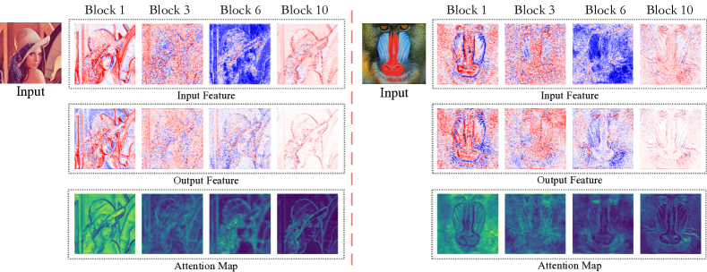
Figure 2: Attention block heatmaps. Due to the limited space, we chose several representative blocks, each columns indicates the first, third, sixth, tenth attention block, respectively. The three rows are averaged input feature map, averaged output feature map, and the averaged attention map for each attention layer, respectively. For the feature maps, the white area in the feature map indicates zero values, the red area indicates positive values, and the blue area indicates negative values. For the attention maps, brighter colors represent a higher attention coefficient.

II-B Attention Mechanism

Attention mechanism in deep learning is similar to the attention mechanism of human vision. It can be viewed as a means of biasing the allocation of available computational resources towards the most informative components of a signal [11]. Attention mechanism usually contains a gating function to generate a feature mask. It has been applied to many computer vision tasks, such as image captioning [35, 5] and image classification [11, 30]. Wang et al. [31] initially proposed non-local operation for capturing long-range dependencies, it computes the response at a position as a weighted sum of the features at all positions. Hu et al. [11] focus on the channel relationship and propose a novel architectural unit, Squeeze-and-Excitation (SE) block, that adaptively recalibrates channel-wise feature responses. Woo et al. [34] provided a study on the combination of channel and spatial attention.

In recent years, several works proposed to investigate the effect of attention mechanism on low-level vision tasks. [21] first attempt to incorporate non-local operations into a recurrent neural network for image restoration. RNAN [39] proposed residual local and non-local attention blocks in the mask branch in order to obtain non-local mixed attention. Channel attention is another popular way to embed attention mechanism. RCAN [38] exploits the interdependencies among feature channels by generating different attention for each channel-wise feature. Some works utilize both channel attention and non-local attention. SAN [7] performed region-level non-local operations for reducing computational burden, and proposed second-order channel attention by considering second-order statistics of features.

III Motivation

Given an intermediate feature map $\mathbf{F}\in\mathbb{R}^{C\times H\times W}$, where $C$, $H$, and $W$ are the number of channels, height, and width of the features, respectively. Attention mechanism infers an attention map function $\mathbf{M}_{\mathbf{A}}$, where $\mathbf{M}_{\mathbf{A}}(\mathbf{F})\in\mathbb{R}^{C^{\prime}\times H^{\prime}\times W^{\prime}}$, the size of $C^{\prime}$, $H^{\prime}$ and $W^{\prime}$ depend on the type of attention function. For example, channel attention generates a 1D ($\mathbb{R}^{C\times 1\times 1}$) channel-wise attention vector [11, 38, 34, 26, 12]. Spatial attention generates a 2D ($\mathbb{R}^{1\times H\times W}$) attention mask, [34, 26, 12]. Channel-spatial attention generates 3D ($\mathbb{R}^{C\times H\times W}$) attention map, [39, 41]. We naturally raise two questions: (1) Which part of an image tends to have a higher or lower attention coefficient? (2) Are attention mechanisms always beneficial to SR models?

III-A Attention Heatmap

TABLE I: The correlation coefficients between the attention map and the output feature of high-pass filters of the corresponding feature map for each attention block. Red/ Blue text: maximum and minimum value. The bottom two rows are the mean and standard deviation of each attention map.

Filter	Correlation Coefficients with the Input Feature
	Block 1	Block 2	Block 3	Block 4	Block 5	Block 6	Block 7	Block 8	Block 9	Block 10
Laplace Operator	-0.270	-0.082	0.323	0.281	0.296	0.158	-0.098	0.100	0.184	0.433
Scharr Operator	-0.395	-0.122	0.398	0.355	0.412	0.206	-0.079	0.073	0.255	0.435
Sobel Operator	-0.393	-0.153	0.371	0.334	0.379	0.175	-0.109	0.090	0.196	0.491
Mean of Attention Map	0.208	0.126	0.078	0.106	0.065	0.035	0.048	0.039	0.051	0.086
Std of Attention Map	0.125	0.070	0.042	0.081	0.055	0.039	0.060	0.039	0.027	0.075

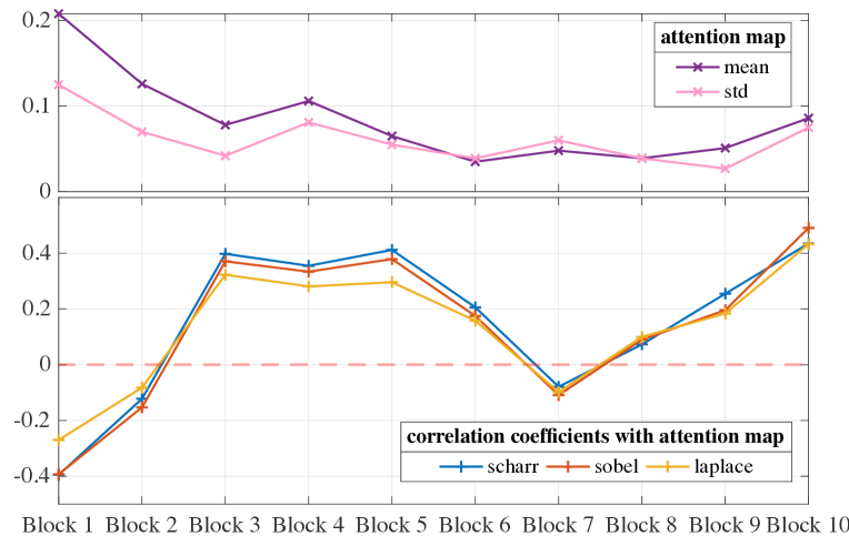
Figure 3: The correlation coefficients between the attention map and the output feature of high-pass filters of the corresponding feature map for each attention block.

TABLE II: Attention layer importance measurement. The first column indicates the insertion stage of the residual attention blocks.

Attention Block Index	# Parameter	PSNR
All	9.2 M	28.65
None	4.4 M	28.60
{1,2,3,4,5}	6.8 M	28.60
{6,7,8,9,10}	6.8 M	28.65
{2,4,6,8,10}	6.8 M	28.63

Previous work [38] suggests that information in the LR space has abundant low-frequency and valuable high-frequency components, all features are treated equally without using the attention mechanism in the networks, while attention can help the network pay more attention to the high-frequency features. The high-frequency components would usually be regions, being full of edges, texture, and other details [38]. However, to our best knowledge, few works truly prove the above assumptions. To answer the first question, we conduct experiments to understand the behavior of the attention mechanism in SR. We construct a simple attention-based model, which consists of ten attention blocks. Each attention block uses a channel- and spatial-wise attention layer so that every pixel has an individual attention coefficient. We use the sigmoid function as the gating function so that the attention coefficient can be scaled into $[0,1]$. We visualize some feature maps and attention maps in Figure 2. TABLE I lists correlation coefficients between the attention map and the high-pass filtering results to the corresponding feature map. Note that this is not a highly accurate method to measure the exact attention response, but our intention is to quantify the relative high-pass correlation across different layers. Based on the observations from the visualized attention maps in Figure 2 and TABLE I, we show that attentions learnt at different layers vary a lot with respect to their relative depth in the neural network. For example, the first and tenth attention blocks show opposite responses. The attention modules in the first two layers tend to enhance the low-frequency bands of the features, while the last two layers enhance the high-frequency features. The blocks in-between have mixed responses.

III-B Ablating Attention

Based on the above results, we may be able to maximize the use of attention while minimizing the number of additional parameters. An intuitive idea is to preserve attention layers only at performance-critical layers. However, the above qualitative analysis is not a valid method to quantify the realistic effect of attention layers. To quantitatively measure the effectiveness of attention layers, we propose a dynamic attention framework. An attention block, regardless of its type mentioned previously in Section II-B, can be downgraded to a non-attentional block by simply removing the attention generator operation.

We have conducted a series of experiments with certain attention layers turned off. The results are shown in TABLE II, where the first column indicates residual attention blocks that are enabled. For example, {1, 2, 3, 4, 5} means attention layers in the first five blocks are residual attention blocks while others are turned off and downgraded to basic residual blocks. The results lead to an interesting result: the relative block depth matters a lot in the decision of where to insert attention blocks. Enabling {6, 7, 8, 9, 10} blocks with attention is effectively achieving the same PSNR as tuning on every block but with much fewer parameters. This experiment further proves that spending budget on attention uniformly across the network is sub-optimal.

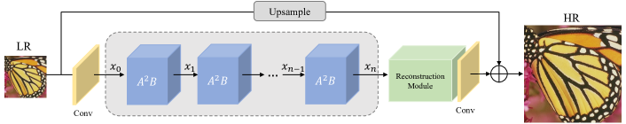
Figure 4: Overview of attention in attention network (A²N).

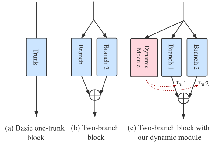
Figure 5: Dynamic Attention Module.

IV Method

Previous models [38, 41, 12] with fixed attention layers have attention maps activated all the time, regardless of image content. We have shown in Sec. III-B that the effectiveness of attention layers varies at different locations in the neural network. Our motivation here is to create non-attentional shortcut branches for counter-part attention branches with mixing weights generated dynamically through an additional evaluation module using the same input features as ordinary layers.

IV-A Network Architecture

As shown in Figure 4, the network architecture of our proposed method, consists of three parts: shallow feature extraction, attention in attention block deep feature extraction, and reconstruction module. The input and output image is denoted as $I_{LR}$ and $I_{SR}$. Follow [20], we use a single convolution layer in shallow feature extraction module. We can then formulate $x_{0}=f_{ext}(I_{LR})$ , where $f_{ext}(\cdot)$ is a convolution layer with 3$\times$3 kernel size to extract the shallow feature from the input LR image $I_{LR}$, $x_{0}$ is the extracted feature map.

We construct our deep feature extractor as a chained sub-network using A²B.

$$x_{n}=f_{A^{2}B}^{n}\left(f_{A^{2}B}^{n-1}\left(\ldots f_{A^{2}B}^{0}\left(x_{0}\right)\ldots\right)\right)$$ (1)

where $f_{A^{2}B}(\cdot)$ denotes the attention in attention block. A²B combines non-attention branch and attention branch with dynamic weights determined by the input feature.

After deep feature extraction, we upscale the deep feature $x_{n}$ via the reconstruction module. In the reconstruction module, we first use nearest-neighbor interpolation for upsampling, then we use a simplified channel-spatial attention layer between two convolution layers. This simplified attention layer only uses one 1 $\times$ 1 convolution and sigmoid function to generate the attention map. We also use global connection, in which a nearest-neighbor interpolation is performed on the input $I_{LR}$. The final model produces high resolution result by applying the reconstruction signal to upsampled output:

$$I_{SR}=f_{rec}(x_{n})+f_{up}(I_{LR})$$ (2)

$f_{rec}(\cdot)$ is the reconstruction module, $f_{up}(\cdot)$ is the bilinear interpolation. $I_{SR}$ is the final SR output.

Figure 6: Architecture of the attention in attention block (A²B).

IV-B Attention in Attention Block (A²B)

We have discussed and dynamic contribution from different attention layers in section III-B, nevertheless, it is infeasible to manually determine the topological structure of attention modules. Inspired by the dynamic kernel [6] which use dynamic convolution to aggregate multiple parallel convolution kernels dynamically based upon their attentions, here we propose a learnable dynamic attention module to automatically drop some unimportant attention features and balance the attention branch and non-attention branch. More specifically, each dynamic attention module controls the dynamic weighted contribution from the attention and the non-attention branch using weighted summation. As depicted in Figure 5. Dynamic attention module generates weights by using the same input feature of its block as two independent branches. Formally, we have:

$$x_{n+1}=f_{1\times 1}(\pi_{n}^{na}\times x_{n}^{na}+\pi_{n}^{attn}\times x_{n}^{attn})$$ (3)

where $x_{n}^{na}$ is the output of non-attention branch, and $x_{n}^{attn}$ is the output of the attention branch. $f_{1\times 1}(\cdot)$ donates 1 $\times$ 1 kernel convolution. $\pi_{na}$ and $\pi_{attn}$ are weights of non-attention branch and attention branch respectively, they are computed by the network according to the input feature, instead of two fixed values which are artificially set.

To compute the dynamic weights, we have:

$$\pi_{n}=f_{da}(x_{n})$$ (4)

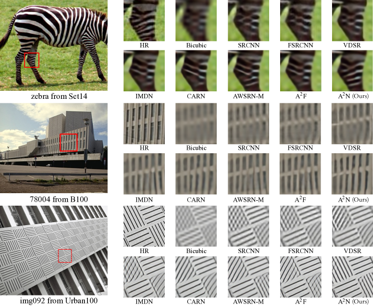
Figure 9: Visual comparison for upscaling factor $\times$4.

where $f_{da}(\cdot)$ is the dynamic attention module. The dynamic attention module can be viewed in detail in Figure 9. It firstly squeezes the input $x_{n-1}$ using global average pooling. The connecting layers consist of two fully connected layers with a ReLU activation. We use global pooling to increase receptive field, which allows dynamic attention module to capture features from the whole image, section 10 gives experiments to prove this. It is worth mentioning that the dynamic attention module is also used in the inference stage, once the input feature changes, the weights of the two branches also change.

As investigated in [6], constraining the dynamic weights can facilitate the learning of the dynamic attention modules. Specifically, we have the sum-to-one constraint $\pi_{n}^{na}+\pi_{n}^{attn}=1$. This sum-to-one constraint for the dynamic weights can compress the kernel space. It significantly simplifies the learning of $\pi$. Therefore, a softmax function is followed to generate normalized attention weights for the two branches.

The overall structure of our proposed attention in attention block in shown in Figure 9. $\bigotimes$ combines feature and attention map by element-wise multiplication, $\bigoplus$ computes weighted summation over two branches as Eq. 3.

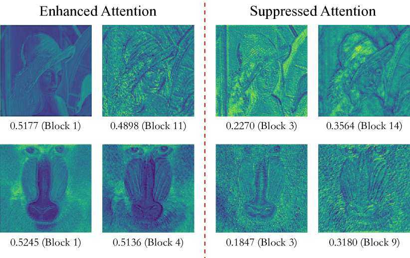
Figure 7: left The most enhanced attention maps. right The most suppressed attention maps. The weight value $\pi^{attn}$ and the block index are shown under the attention maps.

V Experiments

TABLE III: The effect of A² structure. Test on Set14 ($\times$ 4).

		Branch		Branch Fusion					Performance
		Non-attention	Attention	Addition	Concatenation	Adaptive-Weight	A2 (1$\times$1 conv)	A2 (3$\times$3 conv)	Parameter (K)	PSNR
	A2N-non-attn-only	$\bullet$							208	28.515
Single branch	A2N-attn-only (baseline)		$\bullet$						810	28.646
	A2N-Addition	$\bullet$	$\bullet$	$\bullet$					1,040	28.651
	A2N-Concatenation	$\bullet$	$\bullet$		$\bullet$				1,092	28.642
Two Branches, without A2	A2N-Adaptive-Weights	$\bullet$	$\bullet$			$\bullet$			1,040	28.648
	A2N-S (Fewer Channels )	$\bullet$	$\bullet$					$\bullet$	678	28.651
	A2N-M	$\bullet$	$\bullet$				$\bullet$		843	28.695
A2	A2N	$\bullet$	$\bullet$					$\bullet$	1,047	28.707

In this section, we compare our method with state-of-the-art SISR algorithms on five commonly used benchmark datasets. Besides, we conduct ablation study to validate and analyze the effectiveness of our proposed method.

V-A Datasets and Metrics

We use DIV2K dataset [1] as our training dataset, which contains 800 training images. The LR images are obtained by the bicubic downsampling of HR images. For testing stage, we use five standard benchmark datasets: Set5[4], Set14[36], B100[24], Urban100[13] and Manga109[25]. The SR results are evaluated by peak signal to noise ratio (PSNR) and the structural similarity index (SSIM) on the Y channel of YCbCr space.

V-B Implementation Details

Now we specify the implementation details of our proposed A²N. We design two variants of A²N, denoted as A²N and A²N-M. On the non-attention branch, we use 3$\times$3 convolution for A²N and 1$\times$1 convolution for A²N-M. For both variants, we set the number of A²B as 16. Features in A²B have 40 filters, except for that in the upsampling block, where C = 24. For the training process, data augmentation is performed on the 800 training images, which are randomly rotated by 90^∘, 180^∘, 270^∘, and flipped horizontally.

V-C Results

TABLE IV: Ablation study: effect of different components. Test on Set14 ($\times$ 4).

Case Index	1	2	3	4	5	6	7	8
non-attention	$\bullet$		$\bullet$	$\bullet$	$\bullet$		$\bullet$	$\bullet$
channel attention	$\bullet$	$\bullet$			$\bullet$	$\bullet$
spatial attention		$\bullet$		$\bullet$		$\bullet$		$\bullet$
channel-spatial attention			$\bullet$				$\bullet$
A2					$\bullet$	$\bullet$	$\bullet$	$\bullet$
Parameter (K)	787	1,035	1,040	791	794	1,042	1,047	798
PSNR	28.634	28.649	28.651	28.583	28.600	28.629	28,707	28.642
Gain from A2	-	-	-	-	-0.034	-0.020	+0.056	+0.059

To demonstrate the effect of our proposed A² structure, we compare our two-branch A² structure with a one-trunk structure. The results are shown in TABLE III. If we only keep the attention branch, similar to previous models, 28.646 dB is obtained with 810K parameters. Using our A² structure, the performance increased by 0.05 dB with only 200K extra parameters; If we reduce the number of channels of our method to 32, A² performs better with 132K fewer parameters. The results also prove once again that not all attention layers are making positive contributions.

We also show results in TABLE IV to evaluate the performance of A² structure on the multi-branch model. Cases 1-4 are two-branch models without A² structure, features from two branches are fused by an addition operation. Cases 5-8 modify cases 1-4 by applying A² structure. As we can see, for cases 1-4, the combination of non-attention and channel-spatial attention has the best performance. Therefore, we use channel-spatial attention in the attention branch. For cases 1-4, the non-attention branch combine with spatial attention or channel-spatial attention (cases 6 and 7) gains more than 0.05 dB by only about 7K parameters cost. Therefore, the dynamic attention module performs well when used in models without pooling or downsampling layers.

We compare our method with various SR methods of similar model sizes: SRCNN [8], FSRCNN [9], DRRN [27], VDSR [15], MemNet [28], IMDN [14], A²F-M [32], AWSRN-M [29], SRMDNF [37], CARN [2], MADNet[18] and DRCN [16]. We also selected 3 large networks for reference, ERN [19], RCAN [38], and EDSR [20]. TABLE VIII shows quantitative comparisons for $\times$2, $\times$3, and $\times$4 SR. Note that we only compare models which have a similar number of parameters to our models in this table. Our A²N can achieve comparable or better results than state-of-the-art methods for all scaling factors. In particular, A²N-M, which has about 200K fewer parameters than A²F-M and AWSRN-M, achieves better results than these models on most datasets. For Manga109 ($\times 3$), the PSNR of A²N-M is 0.15 dB higher than the PSNR of AWSRN-M. For more difficult scenarios, such as scales 3 and 4, the advantages of our method are more obvious. The performance on more challenging datasets such as Urban100 and Manga109 is more than 0.2 dB higher than that of IMDN.

It should be noted that our core contribution is to dynamically adjust attention to make it play a greater potential, not in terms of lightweight. Therefore, we have not made improvements in terms of lightweight. And in order to better prove the effectiveness of our Dynamic Attention Module, we also did not make a special design for the attention branch, but used the simplest channel-spatial attention. We prove the effectiveness of the Dynamic Attention Module in sections 1 and 2 below, and prove its effect on large models in section 3.

Figure 7 shows the visual comparison for upscaling factor $\times$4. We can see that our method achieves better performance than others, it can recover high frequency details more accurately. For image “zebra”, our method can restore zebra stripes accurately. For the details of the buildings, in image ”78004”, the windows are restored more clearly and accurately. For image ”img092”, only our method can restore the direction of the fringe correctly.

V-D Discussion

We use the weight prediction in the dynamic attention layer to sample the enhanced and suppressed attention signals. Figure 7 shows the two attention maps with the top two weights and the two attention maps with the smallest weights. For each row, the attention maps selected by the highest and second-highest weights are listed on the left, while the right depicts the two attention maps with the smallest weights. As we can see, for attention maps with high weights, the edge and texture components of the feature map can be accurately located, while the attention maps with lower weights can not found it accurately. These results demonstrate the effectiveness of the dynamic attention module, which can automatically determine the weights of the two branches based on the input features.

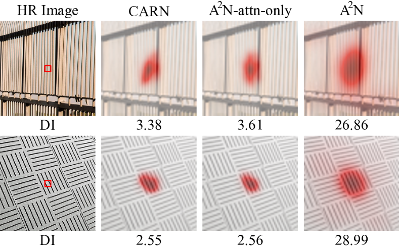
Figure 8: Results of the LAM for SR network interpretation. The LAM maps represent the importance of each pixel in the input LR image w.r.t. the SR of the patch marked with a red box. We illustrate the area of contribution in red color.

TABLE V: Results of different methods used in non-attention branch. A²N-attn-only: no non-attention branch. A²N-no-op: pass through in non-attention branch. Test on Set14 ($\times$ 4).

Method	Operation	Parameter	PSNR
A2N-attn-only	-	810K	28.646
A2N-no-op	-	817K	28.660
A2N-M	1 $\times$ 1 Conv	843K	28.695
A2N	3 $\times$ 3 Conv	1047K	28.707

TABLE VI: Test on 150 images which are proposed from LAM [10]. The DI reflects the range of involved pixels. A higher DI represents a wider range of attention.

Model	DI	PSNR
FSRCNN	0.797	20.30
CARN	1.807	21.27
IMDN	14.643	21.23
A2F	12.58	21.43
A2N-attn-only	2.54	21.33
A2N-non-attn-only	1.56	20.99
A2N-Addition	2.75	21.37
A2N-Concatenation	2.70	21.38
A2N-AdaptiveWeights	2.43	21.33
A2N	14.77	21.44

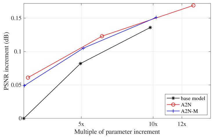
Figure 10: Results of base model and our A² structure on different model size. Our method can get higher PSNR under the similar parameter number.

Comparison with Other Fusion Methods. Most SR models fuse features by addition [17] or concatenation [14, 41]. Some methods [16, 32, 29] give adaptive weights to each feature, which means the independent weights will be learned automatically when training the model. To demonstrate the effectiveness of our method, we compare our dynamic attention module with other mainstream feature fusion methods: addition, concatenation, and adaptive weights. TABLE III shows that within a similar parameter number, A² structure has a considerable improvement over other fusion methods. If we reduce the channel number to 32, even with about 400K fewer parameters, A²N can still obtain a better result than other fusion Methods. It demonstrates that the dynamic attention module is a better feature fusion method than other methods.

Results of Local Attribution Maps. The proposed method can make good use of the information in the input LR image. Recently, Gu et al [10] propose a novel attribution approach called local attribution map (LAM), which performs attribution analysis of SR networks and aims at finding the input pixels that strongly influence the SR results. The results are summarised to diffusion index (DI), an evaluation metric that measures the ability of extraction and utilization of the information in the LR image. A larger DI indicates more pixels are involved. LAM highlights the pixels which have the greatest impact on the SR results. For the same local patch, if the LAM map involves more pixels or a larger range, it can be considered that the SR network has extracted and used the information from more pixels. We follow the suggested setting, and in TABLE VI we show the PSNR and DI performances for some SR networks test on these images. Among all the models, A²N has the highest DI and PSNR. We can notice that using the dynamic attention module makes DI much higher than other models. Figure 8 shows the LAM results, which visualize the importance of pixels. The LAM results indicate that CARN and channel-spatial attention model only utilize very limited information, Our A²N can utilize a wider range of information for better SR results for models without downsampling.

TABLE VII: Results of base model and our A² structure on different model size. The baseline model denotes models with only one attention trunk. Test on Set14 ($\times$ 4).

#channel	#block	Model	PSNR
40	16	baseline	28.646
		A2N-M	28.695 (+0.049)
		A2N	28.707 (+0.061)
64	32	baseline	28.728 (+0.082)
		A2N-M	28.751 (+0.105)
		A2N	28.769 (+0.123)
64	64	baseline	28.782 (+0.136)
		A2N-M	28.797 (+0.151)
		A2N	28.815 (+0.169)

V-E Ablation Study

Choice of channel width in Non-attention Branch. In A²N, we use 3 $\times$ 3 convolution to extract features, in A²N-M, 1 $\times$ 1 convolution is used. We compare the results of 1 $\times$ 1 convolution, 3 $\times$ 3 convolution, and pass-through. From our experimental results shown in TABLE V, even without any operations, A² structure is still better than the one-trunk attention structure. Compare with the one-trunk structure and 1 $\times$ 1 convolution, 1 $\times$ 1 convolution gain 0.049 dB improvement with only 33K parameters. It achieves a great trade-off between parameter number and performance. The results of w/o operation and 1 $\times$ 1 convolution also prove that convolution in non-attention branch truly contributes to the network, it can extract the effective features that the attention branch cannot extract, so that it can complement the features of attention branch. These comparisons firmly demonstrate the effectiveness of A² structure.

TABLE VIII: Quantitative results (PSNR/SSIM) of state-of-the-art SR methods for all upscaling factors $\times$2, $\times$3, and $\times$4. Red/ Blue text: best/second-best among all methods (excluding models with parameters greater than 2M).

Scale	Size Scope	Model	Params	MutiAdds	Set5	Set14	B100	Urban100	Manga109
		FSRCANN [9]	0.01M	6G	37.00/0.9558	32.63/0.9088	31.53/0.8920	29.88/0.9020	36.67/0.9710
		SRCNN [8]	0.06M	52.7G	36.66/0.9542	32.45/0.9067	31.36/0.8879	29.50/0.8946	35.60/0.9663
		DRRN [27]	0.3M	6797G	37.74/0.9591	33.23/0.9136	32.05/0.8973	31.23/0.9188	37.92/0.9760
		VDSR [15]	0.7M	612.6G	37.53/0.9587	33.03/0.9124	31.90/0.8960	30.76/0.9140	37.22/0.9729
		MemNet [28]	0.7M	2662.4G	37.78/0.9597	33.28/0.9142	32.08/0.8978	31.31/0.9195	-
		IMDN [14]	0.7M	158.8G	38.00/0.9605	33.63/0.9177	32.19/0.8996	32.17/0.9283	38.88/ 0.9774
		A2N-M (Ours)	0.8M	200.3G	38.06/0.9601	33.73/ 0.9190	32.22/0.8997	32.34/ 0.9300	38.80/0.9765
		MADNet-$L_{F}$ [18]	0.9M	187.1G	37.85/0.9600	33.39/0.9161	32.05/0.8981	31.59/0.9234	-
	<1M	A2F-M [32]	1M	224.2G	38.04/ 0.9607	33.67/0.9184	32.18/0.8996	32.27/0.9294	38.87/ 0.9774
		A2N (Ours)	1M	247.5G	38.06/ 0.9608	33.75/ 0.9194	32.22/ 0.9002	32.43/ 0.9311	38.87/0.9769
		AWSRN-M [29]	1M	244.1G	38.04/0.9605	33.66/0.9181	32.21/ 0.9000	32.23/0.9294	38.66/0.9772
		SRMDNF [37]	1.5M	347.7G	37.79/0.9600	33.32/0.9150	32.05/0.8980	31.33/0.9200	-
		CARN[2]	1.6M	222.8G	37.76/0.9590	33.52/0.9166	32.09/0.8978	31.92/0.9256	-
	<2M	DRCN [16]	1.8M	17974G	37.63/0.9588	33.04/0.9118	31.85/0.8942	30.75/0.9133	37.63/0.9723
		ERN [19]	9.5M	-	38.18/0.9610	33.88/0.9195	32.30/0.9011	32.66/0.9332	-
		RCAN [38]	16M	-	38.27/0.9614	34.12/0.9216	32.41/0.9027	33.34/0.9384	39.44/0.9786
2	>9M	EDSR [20]	40.7M	-	38.11/0.9602	33.92/0.9195	32.32/0.9013	32.93/0.9351	39.10/0.9773
		FSRCANN [9]	0.01M	6G	37.00/0.9558	32.63/0.9088	31.53/0.8920	29.88/0.9020	36.67/0.9710
		SRCNN [8]	0.06M	52.7G	32.75/0.9090	29.28/0.8209	28.41/0.7863	26.24/0.7989	30.59/0.9107
		DRRN [27]	0.3M	6797G	34.03/0.9244	29.96/0.8349	28.95/0.8004	27.53/0.8378	32.74/0.9390
		VDSR [15]	0.7M	612.6G	33.66/0.9213	29.77/0.8314	28.82/0.7976	27.14/0.8279	32.01/0.9310
		MemNet [28]	0.7M	2662.4G	34.09/0.9248	30.00/0.8350	28.96/0.8001	27.56/0.8376	-
		IMDN [14]	0.7M	71.5G	34.36/0.9270	30.32/0.8417	29.09/0.8046	28.17/0.8519	33.61/0.9445
		A2N-M (Ours)	0.8M	96.6G	34.50/ 0.9279	30.41/ 0.8438	29.13/0.8058	28.35/ 0.8563	33.79/ 0.9458
	<1M	MADNet-$L_{F}$ [18]	0.9M	88.4G	34.14/0.9251	30.20/0.8395	28.98/0.8023	27.78/0.8439	-
		A2F-M [32]	1M	100G	34.50/0.9278	30.39/0.8427	29.11/0.8054	28.28/0.8546	33.66/0.9453
		A2N (Ours)	1M	117.5G	34.47/ 0.9279	30.44/ 0.8437	29.14/ 0.8059	28.41/ 0.8570	33.78/ 0.9458
		AWSRN-M [29]	1.1M	116.6G	34.42/0.9275	30.32/0.8419	29.13/ 0.8059	28.26/0.8545	33.64/0.9450
		SRMDNF [37]	1.5M	156.3G	34.12/0.9250	30.04/0.8370	28.97/0.8030	27.57/0.8400	-
		CARN[2]	1.6M	118.8G	34.29/0.9255	30.29/0.8407	29.06/0.8034	28.06/0.8493	-
	<2M	DRCN [16]	1.8M	17974G	33.82/0.9226	29.76/0.8311	28.80/0.7963	27.15/0.8276	32.31/0.9328
		ERN [19]	9.5M	-	34.62/0.9285	30.51/0.8450	29.21/0.8080	28.61/0.8614	-
		RCAN [38]	16M	-	34.74/0.9299	30.65/0.8482	29.32/0.8111	29.09/0.8702	34.44/0.9499
3	>9M	EDSR [20]	43.1M	-	34.65/0.9280	30.52/0.8462	29.25/0.8093	28.80/0.8653	34.17/0.9476
		FSRCANN [9]	0.01M	4.6G	30.71/0.8657	27.59/0.7535	26.98/0.7150	24.62/0.7280	27.90/0.8517
		SRCNN [8]	0.06M	52.7G	30.48/0.8628	27.49/0.7503	26.90/0.7101	24.52/0.7221	27.66/0.8505
		DRRN [27]	0.3M	6797G	31.68/0.8888	28.21/0.7720	27.38/0.7284	25.44/0.7638	29.46/0.8960
		VDSR [15]	0.7M	612.6G	31.35/0.8838	28.01/0.7674	27.29/0.7251	25.18/0.7524	28.83/0.8809
		MemNet [28]	0.7M	2662.4G	31.74/0.8893	28.26/0.7723	27.40/0.7281	25.50/0.7630	-
		IMDN [14]	0.7M	40.9G	32.21/0.8948	28.58/0.7811	27.56/0.7353	26.04/0.7838	30.45/0.9075
	<1M	A2N-M (Ours)	0.8M	60.6G	32.27/ 0.8963	28.70/ 0.7842	27.61/ 0.7376	26.28/ 0.7919	30.59/ 0.9103
		MADNet-$L_{F}$ [18]	1M	54.1G	32.01/0.8925	28.45/0.7781	27.47/0.7327	25.77/0.7751	-
		A2F-M [32]	1M	56.7G	32.28/0.8955	28.62/0.7828	27.58/0.7364	26.17/0.7892	30.57/0.9100
		A2N (Ours)	1M	72.4G	32.30/0.8966	28.71/ 0.7842	27.61/ 0.7374	26.27/ 0.7920	30.67/ 0.9110
		AWSRN-M [29]	1.3M	72G	32.21/0.8954	28.65/0.7832	27.60/0.7368	26.15/0.7884	30.56/0.9093
		SRMDNF [37]	1.6M	89.3G	31.96/0.8930	28.35/0.7770	27.49/0.7340	25.68/0.7730	-
		CARN[2]	1.6M	90.9G	32.13/0.8937	28.60/0.7806	27.58/0.7349	26.07/0.7837	-
	<2M	DRCN [16]	1.8M	17974G	31.53/0.8854	28.02/0.7670	27.23/0.7233	25.14/0.7510	28.98/0.8816
		ERN [19]	9.5M	-	32.39/0.8975	28.75/0.7853	27.70/0.7398	26.43/0.7966	-
		RCAN [38]	16M	-	32.63/0.9002	28.87/0.7889	27.77/0.7436	26.82/0.8087	31.22/0.9173
4	>9M	EDSR [20]	43.7M	-	32.46/0.8968	28.80/0.7876	27.71/0.7420	26.64/0.8033	31.02/0.9148

Results on Large Model. We conduct experiments on three different sizes of models to analyse the effectiveness of our A² structure. We chose the model which only keeps the attention branch to compare with A²N. We change the number of channels and A²B and get three sizes of models: large, medium, and small. From our experimental results shown in TABLE VII and Figure 10, smaller models with A² structure will gain more bonus than larger models, since for large models the PSNR tends to be saturated. A² structure could also conspicuously improve their performance for large models. Note that the cost of A² structure is almost negligible, these improvements are outstanding. From Figure 10, our method can always get higher PSNR under a similar parameter number.

VI Conclusions

In this work, we show that not all attention modules are equally beneficial, the use of some attention modules can even cause a performance drop. The findings can help later people better use and understand attention in image super-resolution tasks. We than propose attention in attention network (A²N) and building block A²B for image SR. A² structure allows for more aggressive pixel-wise attention adjustments and could dynamically adjust the contribution of attention layers, allowing them to be penalized less frequently. Experiments have demonstrated that our method could achieve superior performances compared with state-of-the-art SR models of similar sizes.

VII Biography Section

Haoyu Chen received his B Eng. degree in computer science and engineering from the Chinese University of Hong Kong, Shenzhen, in 2021. His research interests include computer vision, image processing and image generation.

Jinjin Gu received his B.Eng. degree in computer science and engineering from the Chinese University of Hong Kong, Shenzhen, in 2020. He is currently pursuing a Ph.D. degree in Engineering and IT with the University of Sydney. His research interests include computer vision, image processing, interpretability of deep learning algorithms and the applications of machine learning in industrial.

Zhi Zhang received his B.S. degree in electronic and information technology from Beijing Jiaotong University, Beijing, China, in 2012, and the M.S. and Ph.D. degrees in computer engineering from the University of Missouri-Columbia, Columbia, MO, USA, in 2014 and 2018, respectively. He joined Amazon AI in 2018 in pursuing highly efficient deep learning frameworks and toolkits. His current research interests include object detection, segmentation, and deep network acceleration.

References

- [1] Eirikur Agustsson and Radu Timofte. Ntire 2017 challenge on single image super-resolution: Dataset and study. In The IEEE Conference on Computer Vision and Pattern Recognition (CVPR) Workshops, July 2017.
- [2] Namhyuk Ahn, Byungkon Kang, and Kyung-Ah Sohn. Fast, accurate, and lightweight super-resolution with cascading residual network. In Proceedings of the European Conference on Computer Vision (ECCV), pages 252–268, 2018.
- [3] Parichehr Behjati, Pau Rodriguez, Armin Mehri, Isabelle Hupont, Carles Fernández Tena, and Jordi Gonzalez. Hierarchical residual attention network for single image super-resolution. arXiv preprint arXiv:2012.04578, 2020.
- [4] Marco Bevilacqua, Aline Roumy, Christine Guillemot, and Marie Line Alberi-Morel. Low-complexity single-image super-resolution based on nonnegative neighbor embedding. 2012.
- [5] Long Chen, Hanwang Zhang, Jun Xiao, Liqiang Nie, Jian Shao, Wei Liu, and Tat-Seng Chua. Sca-cnn: Spatial and channel-wise attention in convolutional networks for image captioning. In Proceedings of the IEEE conference on computer vision and pattern recognition, pages 5659–5667, 2017.
- [6] Yinpeng Chen, Xiyang Dai, Mengchen Liu, Dongdong Chen, Lu Yuan, and Zicheng Liu. Dynamic convolution: Attention over convolution kernels. In Proceedings of the IEEE/CVF Conference on Computer Vision and Pattern Recognition, pages 11030–11039, 2020.
- [7] Tao Dai, Jianrui Cai, Yongbing Zhang, Shu-Tao Xia, and Lei Zhang. Second-order attention network for single image super-resolution. In Proceedings of the IEEE conference on computer vision and pattern recognition, pages 11065–11074, 2019.
- [8] Chao Dong, Chen Change Loy, Kaiming He, and Xiaoou Tang. Image super-resolution using deep convolutional networks. IEEE transactions on pattern analysis and machine intelligence, 38(2):295–307, 2015.
- [9] Chao Dong, Chen Change Loy, and Xiaoou Tang. Accelerating the super-resolution convolutional neural network. In European conference on computer vision, pages 391–407. Springer, 2016.
- [10] Jinjin Gu and Chao Dong. Interpreting super-resolution networks with local attribution maps. In Proceedings of the IEEE/CVF Conference on Computer Vision and Pattern Recognition, 2021.
- [11] Jie Hu, Li Shen, and Gang Sun. Squeeze-and-excitation networks. In Proceedings of the IEEE conference on computer vision and pattern recognition, pages 7132–7141, 2018.
- [12] Yanting Hu, Jie Li, Yuanfei Huang, and Xinbo Gao. Channel-wise and spatial feature modulation network for single image super-resolution. IEEE Transactions on Circuits and Systems for Video Technology, 30(11):3911–3927, 2019.
- [13] Jia-Bin Huang, Abhishek Singh, and Narendra Ahuja. Single image super-resolution from transformed self-exemplars. In Proceedings of the IEEE conference on computer vision and pattern recognition, pages 5197–5206, 2015.
- [14] Zheng Hui, Xinbo Gao, Yunchu Yang, and Xiumei Wang. Lightweight image super-resolution with information multi-distillation network. In Proceedings of the 27th ACM International Conference on Multimedia, pages 2024–2032, 2019.
- [15] Jiwon Kim, Jung Kwon Lee, and Kyoung Mu Lee. Accurate image super-resolution using very deep convolutional networks. In Proceedings of the IEEE conference on computer vision and pattern recognition, pages 1646–1654, 2016.
- [16] Jiwon Kim, Jung Kwon Lee, and Kyoung Mu Lee. Deeply-recursive convolutional network for image super-resolution. In Proceedings of the IEEE conference on computer vision and pattern recognition, pages 1637–1645, 2016.
- [17] Jun-Hyuk Kim, Jun-Ho Choi, Manri Cheon, and Jong-Seok Lee. Ram: Residual attention module for single image super-resolution. arXiv preprint arXiv:1811.12043, 2, 2018.
- [18] Rushi Lan, Long Sun, Zhenbing Liu, Huimin Lu, Cheng Pang, and Xiaonan Luo. Madnet: A fast and lightweight network for single-image super resolution. IEEE transactions on cybernetics, 51(3):1443–1453, 2020.
- [19] Rushi Lan, Long Sun, Zhenbing Liu, Huimin Lu, Zhixun Su, Cheng Pang, and Xiaonan Luo. Cascading and enhanced residual networks for accurate single-image super-resolution. IEEE Transactions on Cybernetics, 51(1):115–125, 2021.
- [20] Bee Lim, Sanghyun Son, Heewon Kim, Seungjun Nah, and Kyoung Mu Lee. Enhanced deep residual networks for single image super-resolution. In Proceedings of the IEEE conference on computer vision and pattern recognition workshops, pages 136–144, 2017.
- [21] Ding Liu, Bihan Wen, Yuchen Fan, Chen Change Loy, and Thomas S Huang. Non-local recurrent network for image restoration. In Advances in Neural Information Processing Systems, pages 1673–1682, 2018.
- [22] Jie Liu, Wenjie Zhang, Yuting Tang, Jie Tang, and Gangshan Wu. Residual feature aggregation network for image super-resolution. In Proceedings of the IEEE/CVF Conference on Computer Vision and Pattern Recognition, pages 2359–2368, 2020.
- [23] Hailong Ma, Xiangxiang Chu, and Bo Zhang. Accurate and efficient single image super-resolution with matrix channel attention network. In Proceedings of the Asian Conference on Computer Vision, 2020.
- [24] David Martin, Charless Fowlkes, Doron Tal, and Jitendra Malik. A database of human segmented natural images and its application to evaluating segmentation algorithms and measuring ecological statistics. In Proceedings Eighth IEEE International Conference on Computer Vision. ICCV 2001, volume 2, pages 416–423. IEEE, 2001.
- [25] Yusuke Matsui, Kota Ito, Yuji Aramaki, Azuma Fujimoto, Toru Ogawa, Toshihiko Yamasaki, and Kiyoharu Aizawa. Sketch-based manga retrieval using manga109 dataset. Multimedia Tools and Applications, 76(20):21811–21838, 2017.
- [26] Jongchan Park, Sanghyun Woo, Joon-Young Lee, and In So Kweon. Bam: Bottleneck attention module. arXiv preprint arXiv:1807.06514, 2018.
- [27] Ying Tai, Jian Yang, and Xiaoming Liu. Image super-resolution via deep recursive residual network. In Proceedings of the IEEE conference on computer vision and pattern recognition, pages 3147–3155, 2017.
- [28] Ying Tai, Jian Yang, Xiaoming Liu, and Chunyan Xu. Memnet: A persistent memory network for image restoration. In Proceedings of the IEEE international conference on computer vision, pages 4539–4547, 2017.
- [29] Chaofeng Wang, Zheng Li, and Jun Shi. Lightweight image super-resolution with adaptive weighted learning network. arXiv preprint arXiv:1904.02358, 2019.
- [30] Fei Wang, Mengqing Jiang, Chen Qian, Shuo Yang, Cheng Li, Honggang Zhang, Xiaogang Wang, and Xiaoou Tang. Residual attention network for image classification. In Proceedings of the IEEE conference on computer vision and pattern recognition, pages 3156–3164, 2017.
- [31] Xiaolong Wang, Ross Girshick, Abhinav Gupta, and Kaiming He. Non-local neural networks. In Proceedings of the IEEE conference on computer vision and pattern recognition, pages 7794–7803, 2018.
- [32] Xuehui Wang, Qing Wang, Yuzhi Zhao, Junchi Yan, Lei Fan, and Long Chen. Lightweight single-image super-resolution network with attentive auxiliary feature learning. In Proceedings of the Asian Conference on Computer Vision, 2020.
- [33] Xintao Wang, Ke Yu, Shixiang Wu, Jinjin Gu, Yihao Liu, Chao Dong, Yu Qiao, and Chen Change Loy. Esrgan: Enhanced super-resolution generative adversarial networks. In Proceedings of the European Conference on Computer Vision (ECCV), pages 0–0, 2018.
- [34] Sanghyun Woo, Jongchan Park, Joon-Young Lee, and In So Kweon. Cbam: Convolutional block attention module. In Proceedings of the European conference on computer vision (ECCV), pages 3–19, 2018.
- [35] Kelvin Xu, Jimmy Ba, Ryan Kiros, Kyunghyun Cho, Aaron Courville, Ruslan Salakhudinov, Rich Zemel, and Yoshua Bengio. Show, attend and tell: Neural image caption generation with visual attention. In International conference on machine learning, pages 2048–2057. PMLR, 2015.
- [36] Jianchao Yang, John Wright, Thomas S Huang, and Yi Ma. Image super-resolution via sparse representation. IEEE transactions on image processing, 19(11):2861–2873, 2010.
- [37] Kai Zhang, Wangmeng Zuo, and Lei Zhang. Learning a single convolutional super-resolution network for multiple degradations. In Proceedings of the IEEE Conference on Computer Vision and Pattern Recognition, pages 3262–3271, 2018.
- [38] Yulun Zhang, Kunpeng Li, Kai Li, Lichen Wang, Bineng Zhong, and Yun Fu. Image super-resolution using very deep residual channel attention networks. In Proceedings of the European Conference on Computer Vision (ECCV), pages 286–301, 2018.
- [39] Y Zhang, K Li, K Li, B Zhong, and Y Fu. Residual non-local attention networks for image restoration. In International Conference on Learning Representations, 2019.
- [40] Yulun Zhang, Yapeng Tian, Yu Kong, Bineng Zhong, and Yun Fu. Residual dense network for image super-resolution. In Proceedings of the IEEE conference on computer vision and pattern recognition, pages 2472–2481, 2018.
- [41] Hengyuan Zhao, Xiangtao Kong, Jingwen He, Yu Qiao, and Chao Dong. Efficient image super-resolution using pixel attention. arXiv preprint arXiv:2010.01073, 2020.