Bayesian Algorithm Execution: Estimating Computable Properties of Black-box Functions Using Mutual Information

Abstract

In many real-world problems, we want to infer some property of an expensive black-box function $f$, given a budget of $T$ function evaluations. One example is budget constrained global optimization of $f$, for which Bayesian optimization is a popular method. Other properties of interest include local optima, level sets, integrals, or graph-structured information induced by $f$. Often, we can find an algorithm $\mathcal{A}$ to compute the desired property, but it may require far more than $T$ queries to execute. Given such an $\mathcal{A}$, and a prior distribution over $f$, we refer to the problem of inferring the output of $\mathcal{A}$ using $T$ evaluations as Bayesian Algorithm Execution (BAX). To tackle this problem, we present a procedure, InfoBAX, that sequentially chooses queries that maximize mutual information with respect to the algorithm’s output. Applying this to Dijkstra’s algorithm, for instance, we infer shortest paths in synthetic and real-world graphs with black-box edge costs. Using evolution strategies, we yield variants of Bayesian optimization that target local, rather than global, optima. On these problems, InfoBAX uses up to 500 times fewer queries to $f$ than required by the original algorithm. Our method is closely connected to other Bayesian optimal experimental design procedures such as entropy search methods and optimal sensor placement using Gaussian processes.

1 Introduction

Many real-world problems can be described as inferring properties of an expensive black-box function $f$, subject to a computational budget of $T$ function evaluations. This class of problems includes global optimization, commonly tackled by Bayesian optimization methods (Shahriari et al., 2015; Frazier, 2018), but it also encompasses many additional problems. For example, in materials science, $f(x)$ may measure the strength of a material with composition specified by $x\in\mathcal{X}$, and the goal might be to find the set of materials with strength above a threshold $C$, without ever evaluating more than $T$ materials, due to the cost of such experiments (Zhong et al., 2020; Tran et al., 2021). Here, the property of interest is a set of points, the superlevel set of $f$.

Often, there exist effective algorithms to compute our property of interest in the absence of a budget constraint. We call such a property a computable property of $f$, if it is the output of an algorithm $\mathcal{A}$ that makes a finite sequence of function evaluations during its execution. In the superlevel set example, $\mathcal{A}$ might simply evaluate $f$ at each $x\in\mathcal{X}$ and output points with $f(x)>C$. Other examples include using numerical quadrature to find integrals of $f$ (Davis and Rabinowitz, 2007), using Newton’s method to find roots of $f$ (Madsen, 1973), using evolution strategies or finite-difference gradient descent to find local optima of $f$, and using Dijkstra’s algorithm to find the shortest path between nodes in a graph when the edge costs are given by $f$ (Dijkstra et al., 1959). The property of interest in these examples take different forms, such as a single value, a set of vectors, or a sequence of edges in a graph. In each case, an algorithm for computing the property exists, but executing that algorithm on $f$ may exceed our budget of $T$ evaluations.

In this paper, we address the general problem of estimating a computable property $O_{\mathcal{A}}:=O_{\mathcal{A}}(f)$ of a black-box function $f$, under a budget constraint $T$, irrespective of the number of evaluations required by the algorithm $\mathcal{A}$. To do this, we posit a probabilistic model for $f$, and use it to estimate $O_{\mathcal{A}}$ given data gathered via function evaluations. Our goal is to make the best $T$ evaluations to yield an accurate estimate. We refer to this problem as Bayesian algorithm execution, or BAX. Note that the probabilistic nature of BAX enables us to work with noisy function evaluations, e.g. $y_{x}\sim f(x)+\mathcal{N}(0,\sigma^{2})$, even if $\mathcal{A}$ is only designed for noiseless settings.

We develop an iterative procedure for BAX, called InfoBAX, that sequentially evaluates the $x\in\mathcal{X}$ that maximizes the mutual information (MI) between $f(x)$ and $O_{\mathcal{A}}$ under our probabilistic model. Each iteration of our procedure can be seen as an instance of Bayesian optimal experimental design (BOED) where we choose an input to make an observation that maximally reduces the uncertainty in the property of interest $O_{\mathcal{A}}$ (Chaloner and Verdinelli, 1995). However, unlike a typical BOED setting, here the randomness in $O_{\mathcal{A}}$ comes completely from the uncertainty in $f$, and $O_{\mathcal{A}}$ is generated by executing algorithm $\mathcal{A}$ on $f$. Thus, we have neither access to a likelihood $p(y\>|\>O_{\mathcal{A}},x)$ nor prior $p(O_{\mathcal{A}})$, as is usually assumed in BOED, leading to computational challenges that we address.

Our procedure relates to BOED methods for Bayesian optimization, such as entropy search methods (Hennig and Schuler, 2012; Hernández-Lobato et al., 2014; Wang and Jegelka, 2017), which leverage a global optimization algorithm to compute a MI objective (our method can be viewed as an extension of this branch of methods to computable function properties, beyond global optima), and also to the MI criterion for optimal sensor placement via Gaussian processes (GPs) (Krause et al., 2008), which we can also view as estimating a certain computable function property. We discuss connections to these methods in Section 2.

All together, our method iteratively evaluates $f$ at $x\in\mathcal{X}$ that maximally reduces the uncertainty, measured by the posterior entropy, of the function property at each step, and can therefore be used to estimate this property using minimal function evaluations. In summary, our contributions are:

• We introduce Bayesian algorithm execution (BAX), the task of inferring a computable property $O_{\mathcal{A}}$ of a black-box function $f$ given an algorithm $\mathcal{A}$ and a prior distribution on $f$, as a general framework that encapsulates many computational problems under uncertainty.

• We present an iterative, MI-maximizing procedure for BAX called InfoBAX, and present effective estimators of the MI objective that rely only on the ability to simulate $\mathcal{A}$ on posterior samples of $f$.

• We demonstrate the applicability of our methods in various settings, including for estimating graph properties (such as shortest paths) via Dijkstra’s algorithm, and local optima (for variants of Bayesian optimization) via evolution strategies.

2 Related Work

Bayesian optimal experimental design

In BOED, we wish to estimate an unknown quantity or statistic $\varphi$ through an observation $y_{x}$ resulting from an action or design $x$. The goal is to choose the design $x$ that results in an observation $y_{x}$ that is most informative about the quantity of interest $\varphi$. Typically, in BOED we assume that we have access to an observation likelihood $p(y_{x}\>|\>\varphi)$ and a prior $p(\varphi)$. One popular strategy is then to maximize the expected information gain (EIG) (Lindley, 1956) about $\varphi$ from observing $y_{x}$. This is equivalent to the mutual information between $\varphi$ and $y_{x}$, which can be written as

$$\operatorname{EIG}(x)=I(y_{x},\varphi)=\mathbb{E}_{p(y_{x}|\varphi)p(\varphi)}\left[\log\frac{p(\varphi\>|\>y_{x})}{p(\varphi)}\right].$$ (1)

The Bayesian optimal design is then $\operatorname*{arg\,max}_{x}\operatorname{EIG}(x)$. In practice, one often uses Monte Carlo or variational approximations of this BOED objective (Chaloner and Verdinelli, 1995; Müller, 2005; Seeger and Nickisch, 2008).

Our setting is similar in structure to sequential BOED but differs in its assumptions of what is computationally available to the practitioner. For us, the unknown quantity $\varphi$ is the output of an algorithm $O_{\mathcal{A}}$, while $y_{x}$ are noisy observations of $f$ at inputs $x$. We can neither compute the likelihood $p(y_{x}\>|\>\varphi)=p(y_{x}\>|\>O_{\mathcal{A}})$ nor the prior $p(\varphi)=p(O_{\mathcal{A}})$, since we allow for arbitrary algorithms $\mathcal{A}$. Furthermore, we cannot even sample from the likelihood for a given $\varphi=O_{\mathcal{A}}$, as in likelihood-free BOED (Drovandi and Pettitt, 2013; Kleinegesse and Gutmann, 2019; Kleinegesse et al., 2020). Recent work (Foster et al., 2019, see Extrapolation example) has also considered special cases of this setting.

BOED for function properties

A number of prior works have presented BOED-based approaches for inferring specific function properties using a probabilistic model for $f$, such as a Gaussian process. Here we focus on two examples which relate closely to our framework: entropy search methods and optimal sensor placement.

Entropy search (ES) methods (Hennig and Schuler, 2012; Hernández-Lobato et al., 2014; Wang and Jegelka, 2017) are Bayesian optimization procedures that can be viewed as BOED, where the function property of interest is $\varphi:=x^{*}:=\operatorname*{arg\,max}_{x\in\mathcal{X}}f(x)$, the global optimizer of $f$. Algorithms for ES typically operate on samples from the posterior distribution over $x^{*}$ (or its value, $f^{*}=f(x^{*})$). To generate these samples, an optimization algorithm is run on posterior samples of $f$, and the sampled outputs of this algorithm allow for Monte Carlo estimates of the BOED MI objective $I(y_{x},x^{*})$ or $I(y_{x},f^{*})$, which is used as an acquisition function to choose subsequent $x_{t}$ to evaluate. Below we will propose procedures for BAX that follow a similar strategy, and can be viewed as extensions of ES methods to computable function properties beyond global optima. We also note that an earlier black-box optimization method known as Informational Approach to Global Optimization (IAGO) (Villemonteix et al., 2009) describes a similar objective as entropy search, albeit with a different computational procedure to approximate this objective.

Another setting related to BOED is the sensor placement problem (Caselton and Zidek, 1984). Given budget of $T$ sensors and a set of potential sensor locations $\mathcal{X}$, we seek to find $X\subseteq\mathcal{X}$ with $|X|=T$ that is “most informative” about the measurement of interest, $f:\mathcal{X}\to\mathbb{R}$. When we measure “informativeness” by the mutual information between $f(X)$ and $f(\overline{X})$, the problem becomes NP-hard. In this setting, Krause et al. (2008) proposed a $1-1/e$ approximation algorithm that iteratively selects the sensor that maximizes the gain in mutual information. The sensor placement problem becomes a special case of BAX when we seek to infer the value of $f$ at fixed locations $X^{\prime}\subseteq\mathcal{X}$ and $\mathcal{A}$ is the algorithm that evaluates $f$ on each $x\in X^{\prime}$.

In addition, there has been work on using BOED methods with GP models to estimate a variety of function properties, which are not based on the above MI objective. For example, the framework of stepwise uncertainty reduction on GPs has led to sampling objectives for tasks such as estimation of level sets or excursion sets (Bect et al., 2012; Chevalier et al., 2014). As another example, the framework of myopic posterior sampling (MPS) (Kandasamy et al., 2019) takes a Thompson sampling-based approach, and has been applied to tasks such as active learning, active posterior estimation, and level set estimation. There have also been methods developed for estimating certain function properties in tasks such as active surveying (Garnett et al., 2012), quadrature (Osborne et al., 2012), sensor set selection (Garnett et al., 2010), and active search of patterns and regions (Ma et al., 2014, 2015).

3 Bayesian Algorithm Execution (BAX)

In Bayesian algorithm execution (BAX), our goal is to estimate $O_{\mathcal{A}}:=O_{\mathcal{A}}(f)\in\mathcal{O}$, the output of an algorithm $\mathcal{A}$ run on a black-box function $f:\mathcal{X}\rightarrow\mathcal{Y}$, by evaluating $f$ on carefully chosen inputs $\{x_{i}\}_{i=1}^{T}\subseteq\mathcal{X}$. We will leverage a probabilistic model for $f$ to guide our choice of $x$, in order to estimate $O_{\mathcal{A}}$ using a minimal number of evaluations.

We assume that our initial uncertainty about the true function is captured by a prior distribution over $f$, denoted by $p(f)$, reflecting our prior beliefs about $f$. One notable example is the case where $p(f)$ is defined by a Gaussian process (GP). Although not strictly necessary, we assume that each observation $y$ of the true function $f_{x}:=f(x)$ at input $x$ is noisy, with $y_{x}\sim f_{x}+\epsilon$ where $\epsilon\sim\mathcal{N}(0,\sigma^{2})$. We denote a dataset of $t-1$ function observations as $\mathcal{D}_{t}=\{(x_{i},y_{x_{i}})\}_{i=1}^{t-1}$, and use $p(f\>|\>\mathcal{D}_{t})$ to denote the posterior distribution over $f$ given observations $\mathcal{D}_{t}$. Given this distribution over $f$, and an algorithm $\mathcal{A}$ that returns as output the computable property of interest $O_{\mathcal{A}}$, we use $p(O_{\mathcal{A}}\>|\>\mathcal{D}_{t})$ to denote the induced posterior distribution over the algorithm output.

Information-based BAX

Under the above assumptions, we propose a sequential procedure to choose inputs that are most informative about the property of interest $O_{\mathcal{A}}$. At each iteration $t$, we have a dataset of observations $\mathcal{D}_{t}$, and we choose an input $x$ that maximizes the mutual information between $O_{\mathcal{A}}$ and the unrevealed observation $y_{x}$. The mutual information between two random variables $A$ and $B$ can be interpreted as the expected information gain about $A$ upon observing $B$. In our case, we choose $x$ to maximize this expected information gain about $O_{\mathcal{A}}$ given $y_{x}$, conditioned on our dataset $\mathcal{D}_{t}$, written

$$\operatorname{EIG}_{t}(x)=\hskip 2.84526pt\mbox{H}\left[O_{\mathcal{A}}\>|\>\mathcal{D}_{t}\right]-{\mathbb{E}}_{p(y_{x}|\mathcal{D}_{t})}\left[\mbox{H}\left[O_{\mathcal{A}}\>|\>\mathcal{D}_{t}\cup\{(x,y_{x})\}\right]\right].$$ (2)

Here, $\mbox{H}\left[O_{\mathcal{A}}\>|\>\mathcal{D}_{t}\right]={\mathbb{E}}_{p(f\>|\>\mathcal{D}_{t})}\left[-\log p(O_{\mathcal{A}}\>|\>\mathcal{D}_{t})\right]$ is the entropy of $p(O_{\mathcal{A}}\>|\>\mathcal{D}_{t})$, and $p(y_{x}\>|\>\mathcal{D}_{t})={\mathbb{E}}_{p(f\>|\>\mathcal{D}_{t})}[p(y_{x}\>|\>f)]$ denotes the posterior predictive distribution at input $x$ after observing data $\mathcal{D}_{t}$. In the following subsections, we will focus on developing practical methods to estimate $\operatorname{EIG}_{t}(x)$.

Similar to methods in Bayesian optimization and sequential BOED, our full procedure is as follows. At each iteration $t$, we use $\operatorname{EIG}_{t}(x)$ as an acquisition function. We optimize this acquisition function to choose the next input to query, i.e. $x_{t}\leftarrow\operatorname*{arg\,max}_{x\in\mathcal{X}}\operatorname{EIG}_{t}(x)$. We then evaluate the function $f$ at $x_{t}$ to observe a value $y_{x_{t}}\sim f_{x_{t}}+\epsilon$, and update our dataset $\mathcal{D}_{t+1}\leftarrow\mathcal{D}_{t}\cup\{(x_{t},y_{x_{t}})\}$, before continuing to iteration $t+1$. We refer to this procedure as InfoBAX (Algorithm 1).

Algorithm execution path

Suppose that when we execute algorithm $\mathcal{A}$ on $f$ to compute $O_{\mathcal{A}}$, there are $S$ function evaluations. We refer to the sequence of function inputs and outputs traversed during the execution of the algorithm as the execution path of $\mathcal{A}$ on $f$, denoted $e_{\mathcal{A}}:=e_{\mathcal{A}}(f):=(z_{s},f_{z_{s}})_{s=1}^{S}$.

Note that each input $z_{s}$ in the execution path may depend on all previous inputs and outputs, e.g. $z_{2}:=z_{2}(z_{1},f_{z_{1}})$, $z_{3}:=z_{3}(z_{1},f_{z_{1}},z_{2},f_{z_{2}})$, and $z_{s}$ $:=$ $z_{1}(z_{1},f_{z_{1}},\ldots,z_{s-1},f_{z_{s-1}})$ in general. For example, algorithm $\mathcal{A}$ may have specifically queried $z_{2}$ during its execution because it observed the value $f(z_{1})$ at $z_{1}$. To highlight the fact that inputs on the execution path have these dependencies, we use the notation $z$, instead of $x$. Likewise, we note that the output of $\mathcal{A}$ is a function of the execution path, i.e. $O_{\mathcal{A}}(f):=O_{\mathcal{A}}(e_{\mathcal{A}}(f))=O_{\mathcal{A}}\left((z_{s},f_{z_{s}})_{s=1}^{S}\right)$.

We will make use of this notion of execution paths to define procedures for computing $\operatorname{EIG}_{t}(x)$. However, we emphasize that our procedures will not run $\mathcal{A}$ on the true $f$. Instead, we will only run $\mathcal{A}$ on function samples $\widetilde{f}$ from $p(f\>|\>\mathcal{D}_{t})$.

Algorithm 1 InfoBAX

Input: dataset $\mathcal{D}_{1}$, distribution $p(f)$, algorithm $\mathcal{A}$

1:for $t=1,\ldots,T$ do

2:     $x_{t}\leftarrow\operatorname*{arg\,max}_{x\in\mathcal{X}}\operatorname{EIG}_{t}(x)$ $\triangleright$ See Equation (2)

3:     $y_{x_{t}}\sim f(x_{t})+\epsilon$ $\triangleright$ Evaluate $f$ at $x_{t}$

4:     $\mathcal{D}_{t+1}\leftarrow\mathcal{D}_{t}\cup\{(x_{t},y_{x_{t}})\}$ $\triangleright$ Update dataset

Output: distribution $p(O_{\mathcal{A}}(f)\>|\>\mathcal{D}_{T+1})$

Example: top-$k$ estimation

Here we introduce a running example that will be used to help illustrate our methods. Suppose we have a finite collection of elements $X\subseteq\mathcal{X}$, where each $x\in X$ has an unknown value $f_{x}$. There are various applications where we care about estimating the top-$k$ elements of $X$ with the highest values, denoted $K^{*}\subseteq X$. For instance, each $x\in X$ could be a candidate formula for concrete with tensile strength $f_{x}$, and we wish to find the top $k$ formulae with the highest strengths. Note that if our budget of evaluations satisfies $T\geq|X|$, we could run the following top-$k$ algorithm $\mathcal{A}$: evaluate $f$ on each $x\in X$, sort $X$ in decreasing order, and return the first $k$ elements. In contrast, since $T<|X|$, our goal will be to choose the best $T$ inputs $x_{1},\ldots,x_{T}$ to query, in order to infer $K^{*}$. For full generality, assume that we can evaluate any $x_{t}\in\mathcal{X}$, so we are not restricted to evaluating only inputs in $X$.

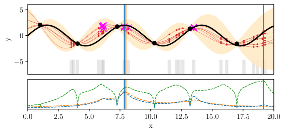
Under algorithm $\mathcal{A}$, the execution path $e_{\mathcal{A}}$ has a fixed sequence of inputs $(z_{1},\ldots,z_{|X|})$ equal to an arbitrary ordering of the $x\in X$. Given a distribution $p(f\>|\>\mathcal{D}_{t})$ over the function $f$ conditioned on some observations $\mathcal{D}_{t}$, we can estimate the top-$k$ elements by executing $\mathcal{A}$ on samples $\widetilde{f}\sim p(f\>|\>\mathcal{D}_{t})$. We illustrate this procedure in Figure 1 for $k=2$. Here, the set $X$ is shown as a set of short grey bars. We also show the true function $f$ (black line), six observations $(x,y_{x})\in\mathcal{D}_{t}$ (black dots), the posterior predictive distribution $p(y_{x}\>|\>\mathcal{D}_{t})$ (tan shaded band), and samples $\widetilde{f}$ (red lines).

Summary of acquisition functions

In the following sections, we present three acquisition functions for InfoBAX, which approximate Eq. (2). First, in Section 3.1, we introduce an acquisition function which is in general suboptimal; however, it will help us define and describe how to compute the latter acquisition functions. After, in Section 3.2, we present an acquisition function which is the optimal quantity that we want, but may be computationally costly to compute. Finally, in Section 3.3, we present an acquisition function that approximates the previous one and is much cheaper to compute, but comes with some restrictions on settings where it should be used.

Figure 1: Illustrations of InfoBAX acquisition functions. Here, $\mathcal{A}$ is the top-$k$ algorithm on a set of elements $X$, for $k=2$ (see text for description). We show the function $f$, elements $x\in X$, observations $(x,y_{x})\in\mathcal{D}_{t}$, posterior predictive distribution $p(y_{x}\>|\>\mathcal{D}_{t})$, posterior samples (of the function $\widetilde{f}$, execution path $\widetilde{e}_{\mathcal{A}}$, and algorithm outputs $\widetilde{O}_{\mathcal{A}}$), and $\operatorname{EIG}$ acquisition functions (4), (8), and (9). The three vertical lines denote the $\operatorname*{arg\,max}$ of the three acquisition functions.

3.1 EIG for the Execution Path

As a first step toward developing our method, we will show how to compute a modified $\operatorname{EIG}$ objective. Note that the execution path $e_{\mathcal{A}}$ is a sequence of $(z_{s},f_{z_{s}})$ pairs which, taken together, give complete information about the algorithm’s output—meaning that if we knew the function value at each point in $e_{\mathcal{A}}$, then we would know the function property $O_{\mathcal{A}}$ exactly. Consequently, one potential strategy for BAX is to, at each iteration, choose to query the $x\in\mathcal{X}$ that gives most information about the execution path (i.e. maximally reduce the entropy of the distribution over $e_{\mathcal{A}}$).

We therefore first present a modified version of the acquisition function $\operatorname{EIG}_{t}(x)$ in (2). Let $\operatorname{EIG}_{t}^{e}(x)$ be the expected gain in information on the execution path $e_{\mathcal{A}}$, written

$$\operatorname{EIG}_{t}^{e}(x)=\hskip 2.84526pt\mbox{H}\left[e_{\mathcal{A}}\>|\>\mathcal{D}_{t}\right]-{\mathbb{E}}_{p(y_{x}|\mathcal{D}_{t})}\left[\mbox{H}\left[e_{\mathcal{A}}\>|\>D_{t}\cup\{(x,y_{x})\}\right]\right].$$ (3)

In the case where the property $O_{\mathcal{A}}=e_{\mathcal{A}}$, this acquisition function is equal to (2), i.e. $\operatorname{EIG}_{t}^{e}(x)=\operatorname{EIG}_{t}(x)$. Otherwise, the two acquisition functions are distinct in general.

There are a few difficulties in computing $\operatorname{EIG}_{t}^{e}(x)$ as it is written in (3). For the first term, we must estimate the entropy of $p(e_{\mathcal{A}}\>|\>\mathcal{D}_{t})$, which is analytically intractable and potentially very high dimensional. If we did have a way to estimate this entropy, we could do the following for the second term for a given $x\in\mathcal{X}$: sample a set of $\widetilde{y}_{x}\sim p(y_{x}\>|\>\mathcal{D}_{t})$, and for each $\widetilde{y}_{x}$ sample, re-train our model on $\mathcal{D}_{t}\cup\{(x,\widetilde{y}_{x})\}$ and estimate the entropy $\mbox{H}\left[e_{\mathcal{A}}\>|\>\mathcal{D}_{t}\cup\{(x,\widetilde{y}_{x})\}\right]$ using the same technique used for the first term. These steps are expensive, and would need to be repeated for each $x\in\mathcal{X}$ over which we intend to optimize our acquisition function.

Instead, we follow an approach from prior work (Hernández-Lobato et al., 2014; Houlsby et al., 2012). Since (3) is the MI between $e_{\mathcal{A}}$ and $y$ (given $\mathcal{D}_{t}$), and due to the symmetry of MI, we can rewrite this acquisition function as

$$\operatorname{EIG}_{t}^{e}(x)=\hskip 2.84526pt\mbox{H}\left[y_{x}\>|\>\mathcal{D}_{t}\right]-{\mathbb{E}}_{p(e_{\mathcal{A}}|\mathcal{D}_{t})}\left[\mbox{H}\left[y_{x}\>|\>\mathcal{D}_{t},e_{\mathcal{A}}\right]\right].$$ (4)

The first term is simply the entropy of the posterior predictive distribution $p(y_{x}\>|\>\mathcal{D}_{t})$, which we can compute exactly for certain probabilistic models such as GPs. For the second term, inside the expectation, we have $\mbox{H}\left[y_{x}\>|\>\mathcal{D}_{t},e_{\mathcal{A}}\right]$, which is the entropy of the posterior predictive distribution at input $x$, given both the dataset $\mathcal{D}_{t}$ and the execution path $e_{\mathcal{A}}$.

Before explaining how to compute $p\left(y_{x}\>|\>\mathcal{D}_{t},e_{\mathcal{A}}\right)$ and its entropy for a given $e_{\mathcal{A}}$, we first describe how to compute the expectation of this entropy with respect to $p(e_{\mathcal{A}}\>|\>\mathcal{D}_{t})$. To do this, we will compute a Monte Carlo estimate via a Thompson sampling-like strategy, related to procedures used by entropy search methods (Hennig and Schuler, 2012; Hernández-Lobato et al., 2014; Wang and Jegelka, 2017). We first draw $\widetilde{f}\sim p(f\>|\>\mathcal{D}_{t})$, and then run our algorithm $\mathcal{A}$ on $\widetilde{f}$ to produce a sample execution path $\widetilde{e}_{\mathcal{A}}=e_{\mathcal{A}}(\widetilde{f})$. Note that this yields a sample $\widetilde{e}_{\mathcal{A}}\sim p(e_{\mathcal{A}}\>|\>\mathcal{D}_{t})$. In Section A.4, we give details on how we implement this procedure for GP models in a computationally efficient manner.

We repeat this multiple times to generate a set of $\ell$ posterior execution path samples $\{\widetilde{e}_{\mathcal{A}}^{\;j}\}_{j=1}^{\ell}$. Notably, unlike the procedure for Eq. (3), we only need to perform this sampling procedure once, and then can use the same set of samples to compute $\operatorname{EIG}_{t}^{e}(x)$ for all $x\in\mathcal{X}$. Concretely, to compute $\operatorname{EIG}_{t}^{e}(x)$, we compute $\mbox{H}[y_{x}\>|\>\mathcal{D}_{t},\widetilde{e}_{\mathcal{A}}^{\;j\;}]$ for each sample $\widetilde{e}_{\mathcal{A}}^{\;j\;}$, and average these to form a Monte Carlo estimate of the second term in Eq. (4), i.e. with $\frac{1}{\ell}\sum_{j=1}^{\ell}\mbox{H}[y_{x}\>|\>\mathcal{D}_{t},\widetilde{e}_{\mathcal{A}}^{\;j\;}]$.

We now describe how to compute $\mbox{H}[y_{x}\>|\>\mathcal{D}_{t},\widetilde{e}_{\mathcal{A}}]$. The key idea is that, under our modeling assumptions, we can derive a closed-form expression for $p(y_{x}\>|\>\mathcal{D}_{t},\widetilde{e}_{\mathcal{A}})$ in which we can compute the entropy analytically. Let the posterior execution path sample $\widetilde{e}_{\mathcal{A}}$ be comprised of the sequence $\widetilde{e}_{\mathcal{A}}=\big{(}\widetilde{z}_{s},\widetilde{f}_{z_{s}}\big{)}_{s=1}^{S}$. We can then show that

$$p\left(y_{x}\>|\>\mathcal{D}_{t},\widetilde{e}_{\mathcal{A}}\right)=p\left(y_{x}\;\Big{|}\;\mathcal{D}_{t},\big{\{}\widetilde{f}_{z_{s}}\big{\}}_{s=1}^{S}\right).$$ (5)

This is equivalent to computing the posterior predictive distribution, given observations with different noise levels, where observations $\mathcal{D}_{t}$ are assumed to have noise given by the likelihood, and variables $\widetilde{f}_{z_{s}}$, are treated as noiseless observations. Under our GP model, this can be computed exactly in closed form (it is a Gaussian distribution), as can $\mbox{H}[y_{x}\>|\>\mathcal{D}_{t},\widetilde{e}_{\mathcal{A}}]$. We show this and give the explicit formula for the GP model in Section A.1.

In Figure 1, we show this acquisition function as the green dashed line. We also show the execution path samples $\widetilde{e}_{\mathcal{A}}^{\;j\;}=e_{\mathcal{A}}(\widetilde{f}^{\;j\;})$, used to compute $\operatorname{EIG}_{t}^{e}$, as red dots over posterior function samples $\widetilde{f}^{\;j}$ (red lines).

We note again that when $O_{\mathcal{A}}\neq e_{\mathcal{A}}$, using $\operatorname{EIG}_{t}^{e}(x)$ in Eq. (4) may be effective in practice, but is suboptimal. For example, given an algorithm where a subsequence of the execution path has no influence on later parts of the execution path nor on the algorithm output, by following the above procedure we may waste queries on estimating portions of $e_{\mathcal{A}}$ that do not give much information about $O_{\mathcal{A}}$.

3.2 EIG for the Algorithm Output

We next show how to use the equations derived above to compute the expected information gain on the algorithm output $O_{\mathcal{A}}$. First, we rewrite the acquisition function $\operatorname{EIG}_{t}(x)$ from Eq. (2) in a predictive entropy-based form (analogous to what was done in Eq. (4)), i.e.

$$\operatorname{EIG}_{t}(x)=\hskip 2.84526pt\mbox{H}\left[y_{x}\>|\>\mathcal{D}_{t}\right]-{\mathbb{E}}_{p(O_{\mathcal{A}}|\mathcal{D}_{t})}\left[\mbox{H}\left[y_{x}\>|\>\mathcal{D}_{t},O_{\mathcal{A}}\right]\right].$$ (6)

Unlike the previous strategy, it is difficult to compute $p(y_{x}\>|\>\mathcal{D}_{t},O_{\mathcal{A}})$ in Eq. (6), in general, for any algorithm $\mathcal{A}$, due to conditioning on the algorithm output $O_{\mathcal{A}}$. This distribution is the posterior predictive at an input $x$ given dataset $\mathcal{D}_{t}$, and also conditioned on the black-box function having property $O_{\mathcal{A}}$. While we can compute $p(y_{x}\>|\>\mathcal{D}_{t},e_{\mathcal{A}})$ in closed form under certain models, since $e_{\mathcal{A}}$ is a sequence of inputs and function values, this is not the case when we condition on $O_{\mathcal{A}}$, which can be an arbitrary property of $f$. However, by using the execution path as an auxiliary variable, we can equivalently write this posterior as

$$p(y_{x}\>|\>\mathcal{D}_{t},O_{\mathcal{A}}) =\int p(y_{x},e_{\mathcal{A}}\>|\>\mathcal{D}_{t},O_{\mathcal{A}})\mathop{}\!\mathrm{d}e_{\mathcal{A}}$$

$$=\int p(y_{x}\>|\>\mathcal{D}_{t},e_{\mathcal{A}},O_{\mathcal{A}})\hskip 2.84526ptp(e_{\mathcal{A}}\>|\>O_{\mathcal{A}},\mathcal{D}_{t})\mathop{}\!\mathrm{d}e_{\mathcal{A}}$$

$$={\mathbb{E}}_{p(e_{\mathcal{A}}|O_{\mathcal{A}},\mathcal{D}_{t})}\left[p\left(y_{x}\>|\>\mathcal{D}_{t},e_{\mathcal{A}}\right)\right].$$ (7)

Here we use the fact that $\mathcal{A}$ defines an execution path that specifies the algorithm output exactly, and thus $y\mathrel{\text{\scalebox{1.07}{$\perp\mkern-10.0mu\perp$}}}O_{\mathcal{A}}\>|\>e_{\mathcal{A}}$. We can therefore write Eq. (6) as

$$\operatorname{EIG}_{t}(x)=\hskip 2.84526pt\mbox{H}\left[y_{x}\>|\>\mathcal{D}_{t}\right]-{\mathbb{E}}_{p(O_{\mathcal{A}}|\mathcal{D}_{t})}\left[\mbox{H}\left[{\mathbb{E}}_{p(e_{\mathcal{A}}|O_{\mathcal{A}},\mathcal{D}_{t})}\left[p\left(y_{x}\>|\>\mathcal{D}_{t},e_{\mathcal{A}}\right)\right]\right]\right].$$ (8)

Given that we have access to $p\left(y_{x}\>|\>\mathcal{D}_{t},e_{\mathcal{A}}\right)$ in closed form, we can estimate the expression ${\mathbb{E}}_{p(e_{\mathcal{A}}\>|\>O_{\mathcal{A}},\mathcal{D}_{t})}\left[p\left(y_{x}\>|\>\mathcal{D}_{t},e_{\mathcal{A}}\right)\right]$ using $\frac{1}{\ell}\sum_{k=1}^{\ell}p\left(y_{x}\>|\>\mathcal{D}_{t},\widetilde{e}_{\mathcal{A}}^{\;k\;}\right)$, where $\widetilde{e}_{\mathcal{A}}^{\;k\;}$ $\stackrel{{\scriptstyle iid}}{{\sim}}$ $p(e_{\mathcal{A}}\>|\>O_{\mathcal{A}},\mathcal{D}_{t})$. By sampling from this, we can approximate the entropy in Eq. (8) via a Monte Carlo estimate. Therefore, the key question is how to draw samples from $p(e_{\mathcal{A}}\>|\>O_{\mathcal{A}},\mathcal{D}_{t})$. Intuitively, a sample $\widetilde{e}_{\mathcal{A}}^{\;k\;}\sim p(e_{\mathcal{A}}\>|\>O_{\mathcal{A}},\mathcal{D}_{t})$ is a plausible execution path, given observations $\mathcal{D}_{t}$, which also yields output $O_{\mathcal{A}}$. At a given iteration of InfoBAX, suppose we generate a set of samples from the posterior over algorithm outputs, $\{\widetilde{O}_{\mathcal{A}}^{\;j\;}\}_{j=1}^{\ell}\stackrel{{\scriptstyle iid}}{{\sim}}p(O_{\mathcal{A}}\>|\>\mathcal{D}_{t})$ by running $\mathcal{A}$ on posterior function samples $\widetilde{f}^{\;j\;}$. Suppose also that we have defined a distance $d(\cdot,\cdot)$ on our algorithm output space $\mathcal{O}$. For each $\widetilde{O}_{\mathcal{A}}^{\;j\;}$, we could then define a set of similar outputs $\mathring{O}_{\mathcal{A}}^{\;j\;}$ to be

$$\mathring{O}_{\mathcal{A}}^{\;j\;}=\left\{\widetilde{O}\in\{\widetilde{O}_{\mathcal{A}}^{\;k\;}\}_{k=1}^{\ell}\;:\;d(\widetilde{O},\widetilde{O}_{\mathcal{A}}^{\;k\;})<\delta,\hskip 2.84526ptk\neq j\right\},$$

i.e. all outputs within a ball of diameter $\delta$ centered at $\widetilde{O}_{\mathcal{A}}^{\;j\;}$. Intuitively, we can then compute the EIG on a ball of diameter $\delta$ in the output space that contains the algorithm output, rather than on the algorithm output directly.

More formally, this can be viewed as an instance of approximate Bayesian computation (ABC) (Beaumont et al., 2002; Csilléry et al., 2010), which is a technique for generating posterior samples, given only a simulator for the likelihood. In our case, by running $\mathcal{A}$, we can simulate an output $O_{\mathcal{A}}$ given an execution path $e_{\mathcal{A}}$, and use this to produce approximate posterior samples from $p(e_{\mathcal{A}}\>|\>O_{\mathcal{A}},\mathcal{D}_{t})$. Concretely, suppose we’ve sampled a set of pairs $P^{j}:=\{(\widetilde{e}_{\mathcal{A}}^{\;j\;},\widetilde{O}_{\mathcal{A}}^{\;j\;})\}$ by running algorithm $\mathcal{A}$ on samples $\widetilde{f}\sim p(f\>|\>\mathcal{D}_{t})$. For each $\widetilde{O}_{\mathcal{A}}^{\;j\;}$, we can then treat $\mathring{e}_{\mathcal{A}}^{\;j\;}=\{e\in P^{j}:\widetilde{O}_{\mathcal{A}}\in\mathring{O}_{\mathcal{A}}^{\;j\;}\}$ as approximate samples from $p(e_{\mathcal{A}}\>|\>\widetilde{O}_{\mathcal{A}}^{\;j\;},\mathcal{D}_{t})$. This is equivalent to the ABC algorithm from Rubin (1984) and Beaumont (2010). We then use the set of sample execution paths $\mathring{e}_{\mathcal{A}}^{\;j\;}$ to construct the sample estimate of $\operatorname{EIG}_{t}(x)$ in (8). We give explicit formulae for (8) under GP models in Section A.2.

As InfoBAX progresses, and we have better estimates of the algorithm output, we can reduce the diameter $\delta$ and continue to yield large enough sample sets $\mathring{e}_{\mathcal{A}}^{\;j\;}$ to form accurate Monte Carlo estimates of (8). In practice, we choose $\delta$ to be the smallest value such that every $\mathring{e}_{\mathcal{A}}^{\;j\;}$ has size greater than a fixed number (such as 30).

In Figure 1, we show this acquisition function as the yellow dashed line. We also show samples of the algorithm output $\widetilde{O}_{\mathcal{A}}^{\;j\;}$ (from which we then produce $\mathring{O}_{\mathcal{A}}^{\;j\;}$) as magenta crosses.

3.3 EIG using an Execution Path Subsequence

One disadvantage of using $\operatorname{EIG}_{t}(x)$ in Eq. (8) is that it may require a large set of samples $\{\widetilde{e}_{\mathcal{A}}^{\;j}\}_{j=1}^{\ell}$ $\stackrel{{\scriptstyle iid}}{{\sim}}$ $p(e_{\mathcal{A}}\>|\>O_{\mathcal{A}},\mathcal{D}_{t})$, in order to compute an accurate Monte Carlo estimate. Instead, one final strategy we can attempt is to determine a latent variable $v$, in which

1. we can draw samples $\widetilde{v}\sim p(v\>|\>\mathcal{D}_{t})$,

2. we can compute $p\left(y_{x}\>|\>\mathcal{D}_{t},\widetilde{v}\right)$, and

3. the EIG with respect to $v$, $\operatorname{EIG}_{t}^{v}(x)\approx\operatorname{EIG}_{t}(x)$.

A potential idea is to try and define a mapping from an execution path $e_{\mathcal{A}}$ to a $v$ that best fits the above criteria. For example, consider a subsequence of $e_{\mathcal{A}}$ of length $R$, denoted $s_{\mathcal{A}}:=s_{\mathcal{A}}(f):=(z_{i_{r}},f_{z_{i_{r}}})_{r=1}^{R}$. We can denote the function values for this subsequence with $v_{\mathcal{A}}:=v_{\mathcal{A}}(f)$ $:=$ $\{f_{z_{r}}\}_{r=1}^{R}$, and then write

$$\operatorname{EIG}_{t}^{v}(x)=\hskip 2.84526pt\mbox{H}\left[y_{x}\>|\>\mathcal{D}_{t}\right]-{\mathbb{E}}_{p(f|\mathcal{D}_{t})}\left[\mbox{H}\left[y_{x}\>|\>\mathcal{D}_{t},\{f_{z_{r}}\}_{r=1}^{R}\right]\right].$$ (9)

Note that the posterior $p\left(y_{x}\>|\>\mathcal{D}_{t},s_{\mathcal{A}}\right)$ $\neq$ $p\left(y_{x}\>|\>\mathcal{D}_{t},v_{\mathcal{A}}\right)$. The former, in general, depends on unconditioned latent variables in the execution path $e_{\mathcal{A}}$, and is intractable to compute (this is not the case, however, when $s_{\mathcal{A}}=e_{\mathcal{A}}$, as we show in (5)). On the other hand, for models such as GPs, $p\left(y_{x}\>|\>\mathcal{D}_{t},v_{\mathcal{A}}\right)$ can indeed be computed exactly and its entropy available in closed form. Hence, $v_{\mathcal{A}}$ satisfies (ii).

Furthermore, to compute samples $\widetilde{v}_{\mathcal{A}}\sim p(v_{\mathcal{A}}\>|\>\mathcal{D}_{t})$ we can easily sample $\widetilde{f}\sim p(f\>|\>\mathcal{D}_{t})$, and then set $\widetilde{v}_{\mathcal{A}}=v_{\mathcal{A}}(\widetilde{f})$, so $v_{\mathcal{A}}$ satisfies (i) as well. Note that, since we can sample $\widetilde{v}_{\mathcal{A}}$ and compute $p\left(y_{x}\>|\>\mathcal{D}_{t},\widetilde{v}_{\mathcal{A}}\right)$, we can estimate $\operatorname{EIG}_{t}^{v}(x)$ via a Monte Carlo estimate similar to (4).

However, we still need to show that $v_{\mathcal{A}}$ satisfies (iii). For this, we focus on a special case of interest. In some problems, the function property $O_{\mathcal{A}}$ exactly specifies some function values $v_{\mathcal{A}}$ along a subsequence $s_{\mathcal{A}}$ of the execution path. A few examples of such properties include optima (where $s_{\mathcal{A}}$ consists of an optima $x^{*}$ and its value $f_{x^{*}}$), level sets (where $s_{\mathcal{A}}$ is the set of $(x,f_{x})$ pairs in a super/sublevel set), function roots (where $s_{\mathcal{A}}$ is a root of $f$), and phase boundaries (where $s_{\mathcal{A}}$ is a set of $(x,f_{x})$ pairs that comprise the phase boundary). In these cases, for a given sample $\widetilde{f}\sim p(f|\mathcal{D}_{t})$ with associated $\widetilde{O}_{\mathcal{A}}$ and $\widetilde{v}_{\mathcal{A}}$, we have that $p(y_{x}\>|\>\mathcal{D}_{t},\widetilde{O}_{\mathcal{A}})$ $=$ $p(y_{x}\>|\>\mathcal{D}_{t},\widetilde{v}_{\mathcal{A}},\widetilde{O}_{\mathcal{A}})$, and

$$p(y_{x}\>|\>\mathcal{D}_{t},\widetilde{v}_{\mathcal{A}})={\mathbb{E}}_{p(O_{\mathcal{A}}|\widetilde{v}_{\mathcal{A}},\mathcal{D}_{t})}\left[p(y_{x}\>|\>\mathcal{D}_{t},\widetilde{v}_{\mathcal{A}},O_{\mathcal{A}})\right]$$

(see Section A.3 for details). $\operatorname{EIG}_{t}^{v}(x)$ will thus serve as a better approximation when $\mbox{H}\left[O_{\mathcal{A}}|v_{\mathcal{A}},\mathcal{D}_{t}\right]$ is small, and will be optimal when $\mbox{H}\left[O_{\mathcal{A}}|v_{\mathcal{A}},\mathcal{D}_{t}\right]=0$, in which case $\operatorname{EIG}_{t}^{v}(x)=\operatorname{EIG}_{t}(x)$.

Empirically, we often observe this behavior. For example, in Figure 1, we show $\operatorname{EIG}_{t}^{v}(x)$ as the blue dashed line, which closely approximates $\operatorname{EIG}_{t}(x)$ (the yellow dashed line). In cases such as those given above, where property $O_{\mathcal{A}}$ specifies some function values $v_{\mathcal{A}}$ along a subsequence of $e_{\mathcal{A}}$, a computationally attractive and practically effective strategy is to use the acquisition function $\operatorname{EIG}_{t}^{v}(x)$ in (9).

4 Experiments

We evaluate our proposed InfoBAX method for Bayesian algorithm execution on three applications in distinct domains. Our experiments demonstrate the generality of the BAX framework for formalizing the task of inferring black-box function properties and the effectiveness of InfoBAX for estimating graph properties, local optima, and top-$k$ sets. In each problem, we use a property-computing algorithm $\mathcal{A}$ that was not designed for settings where we have a limited budget of function evaluations. Nevertheless, our InfoBAX procedure lets us apply such algorithms under a budget constraint, allowing us to infer the true algorithm output using significantly fewer queries than the algorithm alone would have required.

We use Gaussian processes as our prior distribution $p(f)$ for all tasks. To reduce computation time of posterior sampling, we use the sampling method proposed by (Wilson et al., 2020) implemented in GPFlow (Matthews et al., 2017) with GPU acceleration. We refer the reader to Section A.5 for additional details on our experimental setup as well as empirical comparisons of our proposed MI objectives.

Figure 2: Estimating shortest paths in graphs: (Top row) A comparison of methods on grid-shaped graphs with edge weights give by a black-box function, visualizing sample shortest paths (blue lines) produced by running Dijkstra’s algorithm on $p(f\>|\>\mathcal{D}_{T+1})$ for each method, given a budget of $T=70$ queries. Black circles are queries, purple squares are starting vertices, yellow squares are destination vertices, pink circles are the next queries, ground truth shortest path is black dashed line. (Middle row) Visualization of the 305 queries required by the full Dijkstra’s algorithm. (Bottom row) The error (sum of normalized polygonal areas between the inferred shortest path and the ground truth shortest path) for each method vs. iteration, averaged over 5 trials.

4.1 Estimating Shortest Paths in Graphs

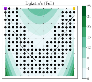
Finding the shortest path between two vertices in a graph is crucial in routing problems, such as minimizing transportation costs, reducing latency when sending packets over the internet, and more. Dijkstra’s algorithm (Dijkstra et al., 1959) provably recovers shortest paths by iteratively querying edge costs as it searches a graph. However, in some applications, querying edge costs is expensive. For example, in transportation networks, when edge costs represent the time required to traverse unfamiliar terrain, it would be costly to survey each location in the order given by Dijkstra’s algorithm. Instead, we may try to survey a small set of locations that provide us with just enough information to map out the shortest path through the terrain, avoiding the full evaluation cost of Dijkstra’s.

As our first task, we use InfoBAX to infer the shortest path between two vertices in a graph where the edge costs are represented by a black-box function. We use two synthetic graphs and one real-world graph for our experiments. Our two synthetic graphs $(V,E)$ are grid-shaped with $(|V|=10\times 10,|E|=684)$ and $(|V|=20\times 10,|E|=2736)$. We use the 2D Rosenbrock function rescaled by $10^{-2}$ as the edge cost function for the synthetic graphs. Our real-world graph is a cropped version of the California roads network graph from Li et al. (2005) and we use the elevation of vertex midpoints from the Open-Elevation API as the edge cost function. Within this graph, we seek to travel from Santa Cruz to Lake Tahoe for a nice change of outdoor activities.

We compare to baseline methods RandomSearch and UncertaintySampling, which choose $\mathcal{D}_{t}$ differently. RandomSearch forms $\mathcal{D}_{t}$ by random queries, while UncertaintySampling iteratively queries $f$ at $x$ that maximize the variance of $p(y_{x}\>|\>\mathcal{D}_{t})$. For InfoBAX, note that we can sample from $p(O_{\mathcal{A}}\>|\>\mathcal{D}_{t})$ by executing algorithm $\mathcal{A}$ on samples from $p(f\>|\>\mathcal{D}_{t})$. Since paths in our experiment consist of points in $\mathcal{X}$, we use the aquisition function from Eq. (9), choosing the points along sampled shortests paths as our execution path subset. To evaluate the error between inferred shortest path and the true shortest path in our planar graph, we use the polygonal area enclosed between the inferred path and the true path. This geometrically captures deviations in the structure of the inferred path from the true path. Notably, an inferred path recovers the ground truth if and only if their enclosed area is zero. We normalize this error metric by the area of the overall graph.

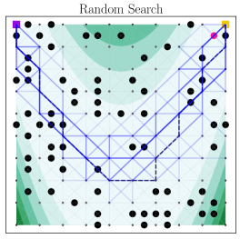
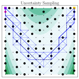
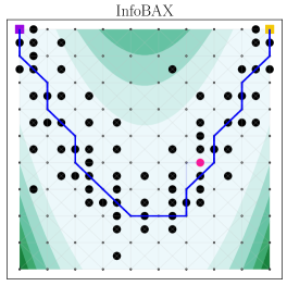
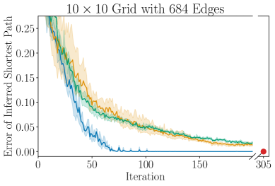
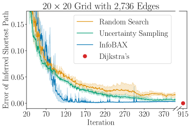
Figure 2 (Top) shows this error metric between the inferred shortest paths and the ground truth, averaged over inferred paths, with one standard error, in three experiments. In all cases, InfoBAX recovers the ground truth shortest path using 5 to 547 times fewer queries than would have been required to run Dijkstra’s algorithm by itself. InfoBAX also outperforms the baseline methods which fail to to recover the ground truth even with significantly more queries.

Figure 2 (Bottom) compares samples from the posterior distribution $p(O_{\mathcal{A}}\>|\>\mathcal{D}_{t})$ given by RandomSearch, UncertaintySampling, and InfoBAX queries. We see that InfoBAX spends its query budget around points that are most informative about the shortest path, as expected. On the other hand, UncertaintySampling queries points that are informative about the overall function $f$ but less informative about the property $O_{\mathcal{A}}$. This behavior can also be seen in Figure 3 on the California roads network.

            

Figure 3: California roads network: (Top row) Visualization of inferences (blue lines) of the true minimum-cost path (black dashed line) given by UncertaintySampling (Left) and InfoBAX (Right) after $T=10$ queries. (Bottom row) The error (sum of normalized polygonal areas between the inferred shortest path and the ground truth shortest path) for each method vs. iteration, averaged over 5 trials.

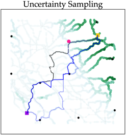
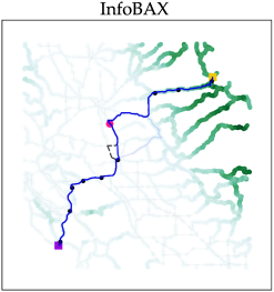
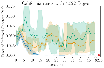
Figure 2 (Top) shows this error metric between the inferred shortest paths and the ground truth, averaged over inferred paths, with one standard error, in three experiments. In all cases, InfoBAX recovers the ground truth shortest path using 5 to 547 times fewer queries than would have been required to run Dijkstra’s algorithm by itself. InfoBAX also outperforms the baseline methods which fail to to recover the ground truth even with significantly more queries.

Figure 2 (Bottom) compares samples from the posterior distribution $p(O_{\mathcal{A}}\>|\>\mathcal{D}_{t})$ by random queries, uncertainty-sampled queries, and InfoBAX queries. We see that InfoBAX spends its query budget around points that are most informative about the shortest path, as expected. On the other hand, UncertaintySampling queries points that are informative about the overall function $f$ but less informative about the property $O_{\mathcal{A}}$. This behavior can also be seen in Figure 3 on the California roads network.

Figure 4: Bayesian local optimization: (Top row) Visualization of function queries and estimated optima for each method, given a budget of $T=18$ queries. Black circles  are function queries, pink stars $\color[rgb]{1,0,1}\definecolor[named]{pgfstrokecolor}{rgb}{1,0,1}\pgfsys@color@cmyk@stroke{0}{1}{0}{0}\pgfsys@color@cmyk@fill{0}{1}{0}{0}\bigstar$ are estimated optima, and yellow squares are the true optima. (Middle row) Queries made by the full EvolutionStrategy algorithm ($T=208$) without InfoBAX. (Bottom row) The difference between the value $f(\hat{x})$ at an estimated optimum $\hat{x}$ and the true optimal value $f(x^{*})$, vs. iteration, on two benchmark tasks.

4.2 Bayesian Local Optimization

Bayesian optimization is a popular method for probabilistic model-based global optimization (Shahriari et al., 2015; Frazier, 2018), that aims to determine global optima of a black-box $f$ in a query-efficient manner. There also exist many local optimization algorithms, such as evolution strategies (Back, 1996), the Nelder-Mead algorithm (Nelder and Mead, 1965), COBYLA (Powell, 1994), and finite-difference gradient descent procedures (Richardson, 1911; Spall et al., 1992), for optimizing a black-box $f$. In certain settings these algorithms have shown very strong performance, such as when $\mathcal{X}$ is high-dimensional, and when function evaluations are cheap and many queries of $f$ can be made (Rios and Sahinidis, 2013). This is potentially because they do not explore as broadly to explicitly try and find a global optima and instead greedily optimize to nearby local optima, or potentially due to other aspects of their updates and how they traverse the space. Regardless, under the right conditions, these algorithms can often be applied to great effect.

However, when function evaluations are expensive, local optimization methods can suffer: these algorithms are often query-inefficient, and may perform a large number of similar evaluations, which hurts performance significantly. Here, Bayesian optimization methods tend to show better performance (Eriksson et al., 2019; Letham et al., 2020). Furthermore, these local methods may not be suited for settings with certain function noise which can be handled more easily in Bayesian optimization via a custom model.

Ideally, we would like the best of both worlds: a procedure that incorporates the model-induced query-efficiency of Bayesian optimization, and also takes advantage of the greedy optimization strategies provided by various local optimization algorithms (which are effective if only they were applied directly to a cheap, noiseless $f$).

We therefore propose running InfoBAX on a local optimization algorithm $\mathcal{A}$, which yields a variant of Bayesian optimization that we refer to as Bayesian local optimization. Here, the main idea is that we approach Bayesian optimization as the task of inferring the output $O_{\mathcal{A}}$ of a local optimization algorithm run on $f$—rather than estimating a global optima of $f$—using as few queries as possible.

We demonstrate this procedure by implementing $\mathcal{A}$ as an evolution strategy, where a population of vectors are randomly mutated and pruned based on their objective values (details given in Section A.5). We compare InfoBAX against this EvolutionStrategy, and also against both RandomSearch and MaxValueEntropySearch (Wang and Jegelka, 2017), which is a popular information-based Bayesian optimization method that aims to efficiently infer global optima of $f$.

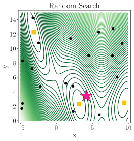
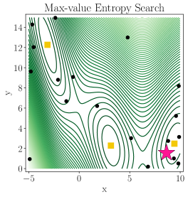
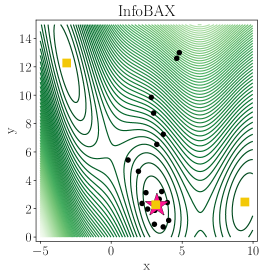
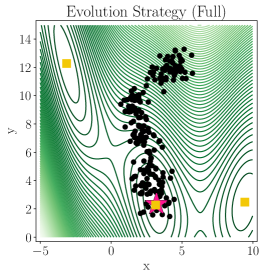
We show results on black-box function optimization benchmark tasks. Figure 4 (Top) compares evaluations chosen by the four methods, where the first three plots show results at $T=18$ iterations, while the fourth plot shows the full EvolutionStrategy ($T=208$). InfoBAX is able to estimate $O_{\mathcal{A}}$ (pink star) using only a fraction of the queries.

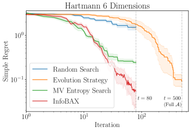
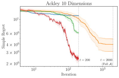
Figure 4 (Bottom) shows the difference between the value of $f(\hat{x})$ at an estimated optimum $\hat{x}$ versus the true optimal value $f(x^{*})$ (over five trials, showing one standard error), on two benchmark functions with domains $\mathcal{X}$ in six and ten dimensions. In both cases, InfoBAX outperforms the baselines and is able to match the eventual performance of the EvolutionStrategy using 8 to 20 times fewer function evaluations.

4.3 Top-$k$ estimation

We show additional experimental results on the problem of top-$k$ estimation. In Section 3, we describe the task of top-$k$ estimation, which we summarize here as follows. Suppose we have a finite collection of elements $X\subseteq\mathcal{X}$, where each $x\in X$ has an unknown value $f_{x}$. There are many applications where we care about estimating the top-$k$ elements of $X$ with the highest values, denoted $K^{*}\subseteq X$. Given a budget $T$, our goal will be to choose the best $T$ inputs $x_{1},\ldots,x_{T}$ to query, in order to infer $K^{*}$. For full generality, assume that we can evaluate any $x_{t}\in\mathcal{X}$, so we are not restricted to evaluating only inputs in $X$. This problem can be viewed as a type of active search, which extends optimization to estimating the top-$k$, rather than top-1, element in a discrete set. It also has relations to level set estimation, where the goal is to estimate all elements $x\in X$ with a value $f_{x}$ above some threshold $C$.

Figure 5: Top-$k$ estimation results: (Top two rows) Visualization of methods, where light grey dots $\color[rgb]{.5,.5,.5}\definecolor[named]{pgfstrokecolor}{rgb}{.5,.5,.5}\pgfsys@color@gray@stroke{.5}\pgfsys@color@gray@fill{.5}\bullet$ are the 150 elements $X\subset\mathcal{X}$ which comprise the execution path $e_{\mathcal{A}}$, black circles are function evaluations, gold stars $\color[rgb]{0.99,0.76,0.0}\definecolor[named]{pgfstrokecolor}{rgb}{0.99,0.76,0.0}\bigstar$ are the true top $k=10$ elements with highest value $f_{x}$, pink circles are the next evaluation chosen, and blue squares are posterior samples of the output (top-$k$ elements). For each method, $T=70$ evaluations are shown. (Bottom row) The Jaccard distance averaged over 5 trials vs. iteration, with error bars showing one standard error.

To run InfoBAX for this problem, we make use of the following top-$k$ algorithm $\mathcal{A}$: evaluate $f_{x}$ for each $x\in X$, sort $X$ in decreasing order, and return the first $k$ elements. This algorithm makes exactly $|X|$ evaluations of $f$. In Figure 1, we illustate the top-$k$ algorithm $\mathcal{A}$, as well as the three acquisition functions in Eqs. (4), (8), and (9).

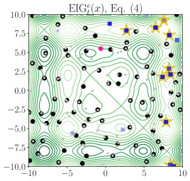
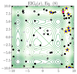
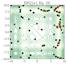
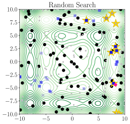
We carry out a top-$k$ estimation experiment on a two dimensional domain $\mathcal{X}\in\mathbb{R}^{2}$, where for each $x\in\mathcal{X}$, $-10<x_{1}<10$, and $-10<x_{2}<10$. From this domain, we draw a set of 150 elements $X$ uniformly at random, and choose to estimate the top $k=10$ elements. For this experiment, we use the skewed sinusoidal function $g:\mathcal{X}\rightarrow\mathbb{R}$, defined as $g(x)=\sum_{i=1}^{d}2|x_{i}|\sin(x_{i})$, which has a multimodal landscape.

Our goal is then to infer $K^{*}\subseteq X$, the top-$k$ elements of $X$, using as few queries of $f$ as possible. We compare the performance of our three InfoBAX acquisition functions ($\operatorname{EIG}_{t}^{e}(x)$, $\operatorname{EIG}_{t}(x)$, and $\operatorname{EIG}_{t}^{v}(x)$), along with RandomSearch and UncertaintySampling (both decribed in Section 4.1), as well as the full top-$k$ algorithm that scans through each point in $X$. For InfoBAX methods, we draw 100 samples of $\widetilde{f}\sim p(f\>|\>\mathcal{D}_{t})$ and run the top-$k$ algorithm $\mathcal{A}$ on these, in order to produce the execution path samples $\widetilde{e}_{\mathcal{A}}$, or algorithm output samples $\widetilde{O}_{\mathcal{A}}$.

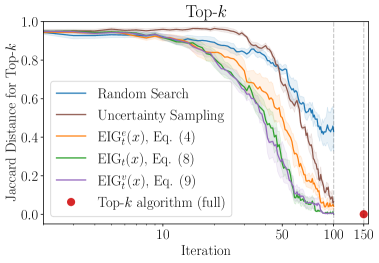
In Figure 5 (Bottom) we show these results, plotting the Jaccard distance for each method at each iteration, which, for a given estimate $\hat{K}$ of the top-$k$ elements of $X$, is defined as

$$\text{Jaccard distance}(\hat{K},K^{*})=1-\text{Jaccard index}(\hat{K},K^{*})=1-\frac{|\hat{K}\cap K^{*}|}{|\hat{K}\cup K^{*}|}.$$ (10)

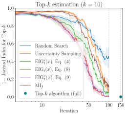
For each method, we average this metric over five trials and show one standard error. The InfoBAX acquisition functions $\operatorname{EIG}_{t}^{v}(x)$ and $\operatorname{EIG}_{t}(x)$ accurately infer the true top-$k$ set in the fewest iterations (using roughly 2 times fewer function evaluations than the full top-$k$ algorithm), followed by InfoBAX using $\operatorname{EIG}_{t}^{e}(x)$, UncertaintySampling, and finally RandomSearch.

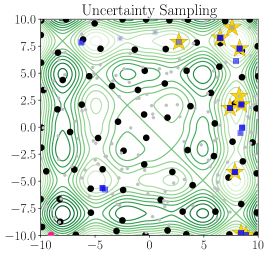
In Figure 5 (Top) we show the set of function evaluations and posterior samples of the inferred top-$k$ sets $\hat{K}$ for each method. We see that InfoBAX, using $\operatorname{EIG}_{t}^{v}(x)$ and $\operatorname{EIG}_{t}(x)$, is able to determine and spend its query budget around the true top-$k$ elements $K^{*}$ (denoted by gold stars). Note also that InfoBAX using $\operatorname{EIG}_{t}^{e}(x)$ focuses its query budget on the execution path $e_{\mathcal{A}}$ (or, equivalently, the set $X$), shown as light grey dots, while UncertaintySampling spends its budget on points that are informative about the full function $f$, as opposed to the execution path $e_{\mathcal{A}}$ or top-$k$ property $O_{\mathcal{A}}$.

5 Conclusion

The BAX framework unifies problems in disparate domains that seek to estimate properties of black-box functions given limited function evaluations. For a property-computing algorithm $\mathcal{A}$, our proposed method, InfoBAX, is able to make targeted queries that can reduce function evaluations by up to hundreds of times without modifying $\mathcal{A}$ to respect the budget constraint. However, InfoBAX also has its limitations. For example, it may be difficult to find an appropriate model $p(f)$, in certain settings. Nevertheless, when we have an accurate function prior, we can dramatically offload the cost of function evaluations to the cost of parallelizable computations. In the future, we hope this branch of methods could potentially aid in custom optimization tasks in the sciences (Char et al., 2019), interactive human-in-the-loop methods (Boecking et al., 2020), and fields such as drug and materials discovery, where function evaluations may be highly expensive or time consuming.

A

In this appendix, we give additional details about the acquisition functions ($\operatorname{EIG}_{t}^{e}(x)$ (4), $\operatorname{EIG}_{t}(x)$ (8), and $\operatorname{EIG}_{t}^{v}(x)$ (9)), discuss the computational cost of InfoBAX, and provide additional experimental details.

A.1 EIG for the Execution Path

Details on equation (5)

Here, we justify more formally the statement given in Eq. (5), used to compute $\operatorname{EIG}_{t}^{e}(x)$, that for an execution path sample $\widetilde{e}_{\mathcal{A}}\sim p(e_{\mathcal{A}}\>|\>\mathcal{D}_{t})$, where $\widetilde{e}_{\mathcal{A}}=(\widetilde{z}_{s},\widetilde{f}_{z_{s}})_{s=1}^{S}$, then

$$p\left(y_{x}\>|\>\mathcal{D}_{t},\widetilde{e}_{\mathcal{A}}\right)=p\left(y_{x}\;\Big{|}\;\mathcal{D}_{t},\big{\{}\widetilde{f}_{z_{s}}\big{\}}_{s=1}^{S}\right).$$

The posterior predictive distribution conditioned on a posterior execution path sample $\widetilde{e}_{\mathcal{A}}$ can be written

$$p\left(y_{x}\>|\>\mathcal{D}_{t},\widetilde{e}_{\mathcal{A}}\right) =p\left(y_{x}\>|\>\mathcal{D}_{t},\widetilde{z}_{1},\widetilde{f}_{z_{1}},\widetilde{z}_{2},\widetilde{f}_{z_{2}},\ldots,\widetilde{z}_{S},\widetilde{f}_{z_{S}}\right)$$

$$=p\left(y_{x}\>|\>\mathcal{D}_{t},\widetilde{z}_{1},\widetilde{f}_{z_{1}},\widetilde{z}_{2}(\widetilde{z}_{1},\widetilde{f}_{z_{1}}),\widetilde{f}_{z_{2}(\widetilde{z}_{1},\widetilde{f}_{z_{1}})},\ldots\right)$$

$$=p\left(y_{x}\>|\>\mathcal{D}_{t},\widetilde{f}_{z_{1}},\widetilde{f}_{z_{2}(\widetilde{z}_{1},\widetilde{f}_{z_{1}})},\ldots\right)$$ (11)

where the third equality holds because each $\widetilde{z}_{s}=\widetilde{z}_{s}(\widetilde{z}_{1},\widetilde{f}_{z_{1}},\ldots)$ is a deterministic function of previous function evaluations $\widetilde{f}_{z_{1}},\ldots,\widetilde{f}_{z_{s-1}}$ in the sequence, as well as the initial $\widetilde{z}_{1}$ (which is assumed to be a determinstic quantity specified by algorithm $\mathcal{A}$), so each $\widetilde{z}_{s}$ can be dropped from the conditioning. Note also that the final line can be written equivalently as $p\left(y_{x}\>|\>\mathcal{D}_{t},\widetilde{f}_{z_{1}},\widetilde{f}_{z_{2}},\ldots\widetilde{f}_{z_{S}}\right)$ $=$ $p\left(y_{x}\;\Big{|}\;\mathcal{D}_{t},\big{\{}\widetilde{f}_{z_{s}}\big{\}}_{s=1}^{S}\right)$.

Background on Gaussian processes

Gaussian processes (GPs) are popular models that are commonly used in Bayesian optimization. In order to give details on Eq. (5) for a Gaussian process model, we first give background on GPs here.

A GP over the input space $\mathcal{X}$ is a random process characterized by a mean function $\mu:\mathcal{X}\rightarrow\mathbb{R}$ and a covariance function (i.e. kernel) $\kappa:\mathcal{X}^{2}\rightarrow\mathbb{R}$. If $f\sim\text{GP}(\mu,\kappa)$, then for all $x\in\mathcal{X}$, we can write the distribution over $f$ at $x$ as $f_{x}\sim\mathcal{N}(\mu(x),\kappa(x,x))$. Suppose that we are given a dataset of $t$ observations $\mathcal{D}_{t}=\{(x_{i},y_{x_{i}})\}_{i=1}^{t}$, where

$$y_{x_{i}}=f_{x_{i}}+\epsilon_{i}\in\mathbb{R}\hskip 5.69054pt\text{and}\hskip 5.69054pt\epsilon_{i}\sim\mathcal{N}(0,\sigma^{2}).$$ (12)

Then the posterior process given $\mathcal{D}_{t}$ is also a GP, with mean function $\mu_{t}$ and covariance function $\kappa_{t}$, which we describe as follows. Let $Y$, $k$, $k^{\prime}\in\mathbb{R}^{t}$ be vectors where $Y_{i}=y_{x_{i}}$, $k_{i}=\kappa(x,x_{i})$, and $k^{\prime}_{i}=\kappa(x^{\prime},x_{i})$. Let $I_{t}\in\mathbb{R}^{t\times t}$ be the identity matrix and let $K\in\mathbb{R}^{t\times t}$ be the Gram matrix with $K_{i,j}=\kappa(x_{i},x_{j})$. Then

$$\mu_{t}(x) =k^{\top}(K+\sigma^{2}I_{t})^{-1}Y,$$ (13)

$$\kappa_{t}(x,x^{\prime}) =\kappa(x,x^{\prime})-k^{\top}(K+\sigma^{2}I_{t})^{-1}k^{\prime}.$$ (14)

Given $\mathcal{D}_{t}$, the posterior predictive distribution for a given $x\in\mathcal{X}$, is $p(y_{x}\>|\>\mathcal{D}_{t})=\mathcal{N}(y_{x}\>|\>\mu_{x},\sigma_{x}^{2})$, where

$$\mu_{x}=\mu_{t}(x)\hskip 5.69054pt\text{and}\hskip 5.69054pt\sigma_{x}^{2}=\kappa_{t}(x,x)+\sigma^{2}.$$ (15)

For additional background on GPs, see Williams and Rasmussen (2006).

Equation (5) for Gaussian processes

Under a GP model, we can derive a closed-form expression for Eq. (5), given dataset $\mathcal{D}_{t}=\{(x_{i},y_{x_{i}})\}_{i=1}^{t}$, and execution path sample $\widetilde{e}_{\mathcal{A}}=(\widetilde{z}_{s},\widetilde{f}_{z_{s}})_{s=1}^{S}$. Intuitively, Eq. (5) is the posterior predictive distribution for a GP with two types of observations: noisy observations $y_{x_{i}}$ and noiseless observations $f_{z_{s}}$. This can be written as

$$p\left(y_{x}\>|\>\mathcal{D}_{t},\widetilde{e}_{\mathcal{A}}\right)=p\left(y_{x}\;\Big{|}\;\mathcal{D}_{t},\big{\{}\widetilde{f}_{z_{s}}\big{\}}_{s=1}^{S}\right)=\mathcal{N}\left(y_{x}\>|\>\widetilde{\mu}_{x},\widetilde{\sigma}_{x}^{2}\right),$$ (16)

where we describe the two parameters $\widetilde{\mu}_{x}$ and $\widetilde{\sigma}_{x}^{2}$ as follows. Let $u=t+S$. Let $\widetilde{Y}\in\mathbb{R}^{u}$ be a vector where

$$\widetilde{Y}_{i}=\begin{cases}y_{x_{i}},&\text{if}\hskip 5.69054pti\in\{1,\ldots,t\}\\ \widetilde{f}_{z_{i-t}}&\text{if}\hskip 5.69054pti\in\{t+1,\ldots,u\}.\end{cases}$$ (17)

Let $\widetilde{k}\in\mathbb{R}^{u}$ be a vector where

$$\widetilde{k}_{i}=\begin{cases}\kappa(x,x_{i}),&\text{if}\hskip 5.69054pti\in\{1,\ldots,t\}\\ \kappa(x,\widetilde{f}_{z_{i-t}})&\text{if}\hskip 5.69054pti\in\{t+1,\ldots,u\},\end{cases}$$ (18)

and define $\widetilde{k}^{\prime}$ similarly. Let $I(\sigma)\in\mathbb{R}^{u\times u}$ be a diagonal matrix, where

$$I(\sigma)_{i,i}=\begin{cases}\sigma,&\text{if}\hskip 5.69054pti\in\{1,\ldots,t\}\\ 0&\text{if}\hskip 5.69054pti\in\{t+1,\ldots,u\}.\end{cases}$$ (19)

Let $\widetilde{K}\in\mathbb{R}^{u\times u}$ be an extended Gram matrix, where

$$\widetilde{K}_{i,j}=\begin{cases}\kappa(x_{i},x_{j}),&\text{if}\hskip 5.69054pti,j\in\{1,\ldots,t\}\\ \kappa(x_{i},\widetilde{z}_{j-t}),&\text{if}\hskip 5.69054pti\in\{1,\ldots,t\},j\in\{t+1,\ldots,u\}\\ \kappa(\widetilde{z}_{i-t},x_{j}),&\text{if}\hskip 5.69054pti\in\{t+1,\ldots,u\},j\in\{1,\ldots,t\}\\ \kappa(\widetilde{z}_{i-t},\widetilde{z}_{j-t}),&\text{if}\hskip 5.69054pti,j\in\{t+1,\ldots,u\}.\end{cases}$$ (20)

Then

$$\widetilde{\mu}_{x} =\widetilde{k}^{\top}(\widetilde{K}+I(\sigma))^{-1}\widetilde{Y},$$ (21)

$$\widetilde{\sigma}_{x}^{2} =\kappa(x,x)-\widetilde{k}^{\top}(\widetilde{K}+I(\sigma))^{-1}\widetilde{k}^{\prime}+\sigma^{2}.$$ (22)

A.2 EIG for the Algorithm Output

In Eq. (8), the $\operatorname{EIG}_{t}(x)$ acquisition function is written

$$\operatorname{EIG}_{t}(x)=\mbox{H}\left[y_{x}\>|\>\mathcal{D}_{t}\right]-{\mathbb{E}}_{p(O_{\mathcal{A}}|\mathcal{D}_{t})}\left[\mbox{H}\left[{\mathbb{E}}_{p(e_{\mathcal{A}}|O_{\mathcal{A}},\mathcal{D}_{t})}\left[p\left(y_{x}\>|\>\mathcal{D}_{t},e_{\mathcal{A}}\right)\right]\right]\right].$$

Here we describe details on how we estimate this acquisition function under a GP model. In Section 3.2, we describe the general procedure: we first draw a set of sample pairs $P^{j}:=\{(\widetilde{e}_{\mathcal{A}}^{\;j\;},\widetilde{O}_{\mathcal{A}}^{\;j\;})\}$, consisting of an execution path and algorithm output, by running algorithm $\mathcal{A}$ on samples $\widetilde{f}\sim p(f\>|\>\mathcal{D}_{t})$. For a given output sample $\widetilde{O}_{\mathcal{A}}^{\;j\;}$, we then carry out an approximate Bayesian computation (ABC)-like procedure to produce a set of execution path samples

$$\mathring{e}_{\mathcal{A}}^{\;j\;}=\{e\in P^{j}:\widetilde{O}_{\mathcal{A}}\in\mathring{O}_{\mathcal{A}}^{\;j\;}\},$$

where $\mathring{O}_{\mathcal{A}}^{\;j\;}$ is a set of similar outputs defined as

$$\mathring{O}_{\mathcal{A}}^{\;j\;}=\left\{\widetilde{O}\in\{\widetilde{O}_{\mathcal{A}}^{\;k\;}\}_{k=1}^{\ell}\;:\;d(\widetilde{O},\widetilde{O}_{\mathcal{A}}^{\;k\;})<\delta,\hskip 2.84526ptk\neq j\right\},$$

and where $d(\cdot,\cdot)$ is some distance function defined on the algorithm output space $\mathcal{O}$. Note that, for a given $e\in\mathring{e}_{\mathcal{A}}^{\;j\;}$, we can compute $p(y_{x}\>|\>\mathcal{D}_{t},e)$ in closed form as described in Section A.1. We can therefore estimate ${\mathbb{E}}_{p(e_{\mathcal{A}}|O_{\mathcal{A}},\mathcal{D}_{t})}\left[p\left(y_{x}\>|\>\mathcal{D}_{t},e_{\mathcal{A}}\right)\right]$ as a mixture density $\frac{1}{|\mathring{e}_{\mathcal{A}}^{\;j\;}|}\sum_{e\in\mathring{e}_{\mathcal{A}}^{\;j\;}}p(y_{x}\>|\>\mathcal{D}_{t},e)$, which in the case of GPs, will be a uniformly weighted mixture of Gaussians. We can easily draw a set of $H$ samples from this mixture of Gaussians to produce a set of one-dimensional samples $\{\widetilde{y}_{x,1}^{\;j\;},\ldots,\widetilde{y}_{x,H}^{\;j\;}\}\subset\mathbb{R}$, and then construct a Monte Carlo estimate of the entropy via $-\frac{1}{H}\sum_{h=1}^{H}\log\left(\frac{1}{|\mathring{e}_{\mathcal{A}}^{\;j\;}|}\sum_{e\in\mathring{e}_{\mathcal{A}}^{\;j\;}}p(\widetilde{y}_{x,h}^{\;j\;}\>|\>\mathcal{D}_{t},e)\right)$.

By following these steps, we produce an estimate of $\mbox{H}\left[{\mathbb{E}}_{p(e_{\mathcal{A}}|\widetilde{O}_{\mathcal{A}}^{\;j\;},\mathcal{D}_{t})}\left[p\left(y_{x}\>|\>\mathcal{D}_{t},e_{\mathcal{A}}\right)\right]\right]$ for $\widetilde{O}_{\mathcal{A}}^{\;j\;}\sim p(O_{\mathcal{A}}\>|\>\mathcal{D}_{t})$, and then can follow the same procedure outlined in Section 3.1 to estimate the full $\operatorname{EIG}_{t}(x)$.

A.3 EIG using an Execution Path Subsequence

Here, we give details on the acquisition function $\operatorname{EIG}_{t}^{v}(x)$ in Eq. (9), which is based on using a set of function values $v_{\mathcal{A}}$ from a subsequence of the execution path. To summarize, let the execution path $e_{\mathcal{A}}=(z_{s},f_{z_{s}})_{s=1}^{S}$ have a subsequence of length $R$, denoted $s_{\mathcal{A}}:=s_{\mathcal{A}}(f):=(z_{i_{r}},f_{z_{i_{r}}})_{r=1}^{R}$. We can denote the function values for this subsequence with $v_{\mathcal{A}}:=v_{\mathcal{A}}(f)$ $:=$ $\{f_{z_{i_{r}}}\}_{r=1}^{R}$.

We focus on the special case where the algorithm output $O_{\mathcal{A}}$ exactly specifies this subsequence $s_{\mathcal{A}}$, as well as its function values $v_{\mathcal{A}}$ (i.e. $s_{\mathcal{A}}$ and $v_{\mathcal{A}}$ are both a deterministic function of $O_{\mathcal{A}}$, and are not random conditioned on $O_{\mathcal{A}}$). There are a number of common applications where we can find such a subsequence, such as in optimization (where $s_{\mathcal{A}}$ consists of an optima $x^{*}$ and its value $f_{x^{*}}$), level set estimation (where $s_{\mathcal{A}}$ is the set of $(x,f_{x})$ pairs in a super/sublevel set), root finding (where $s_{\mathcal{A}}$ is a root of $f$), and phase mapping (where $s_{\mathcal{A}}$ is a set of $(x,f_{x})$ pairs that comprise a phase boundary). Additionally, the three applications that we show in Section 4—estimating shortest paths in graphs, Bayesian local optimization, and top-$k$ estimation—also fall into this setting. In the first case, the subsequence is the sequence of edges and edge-costs that comprise the minimum-cost path in a graph, and in the latter two cases, the subsequence is the optima and associated function value(s).

Given this subsequence $s_{\mathcal{A}}$, and its corresponding function values $v_{\mathcal{A}}$, we then propose using the following acquisition function:

$$\operatorname{EIG}_{t}^{v}(x) =\hskip 5.69054pt\mbox{H}\left[y_{x}\>|\>\mathcal{D}_{t}\right]-{\mathbb{E}}_{p(f|\mathcal{D}_{t})}\left[\mbox{H}\left[y_{x}\>|\>\mathcal{D}_{t},v_{\mathcal{A}}\right]\right].$$

$$=\hskip 5.69054pt\mbox{H}\left[y_{x}\>|\>\mathcal{D}_{t}\right]-{\mathbb{E}}_{p(f|\mathcal{D}_{t})}\left[\mbox{H}\left[y_{x}\>|\>\mathcal{D}_{t},\{f_{z_{i_{r}}}\}_{r=1}^{R}\right]\right].$$

Under a GP model, we can compute this acquisition function in closed form, using Eq. (5), originally derived for the $\operatorname{EIG}_{t}^{e}(x)$ acquisition function (note that this fact is not true if we want to compute the $\operatorname{EIG}$ with respect to the subsequence $s_{\mathcal{A}}$, and that, in general, the posterior predictive $p\left(y_{x}\>|\>\mathcal{D}_{t},s_{\mathcal{A}}\right)$ $\neq$ $p\left(y_{x}\>|\>\mathcal{D}_{t},v_{\mathcal{A}}\right)$).

Next we discuss why this acquisition function shows strong performance in practice. Ideally, we would like to determine $v_{\mathcal{A}}$ such that $\operatorname{EIG}_{t}^{v}(x)$ best approximates $\operatorname{EIG}_{t}(x)$. We can see that

$$\operatorname{EIG}_{t}^{v}(x)-\operatorname{EIG}_{t}(x)={\mathbb{E}}_{p(f\>|\>\mathcal{D}_{t})}\left[\mbox{H}\left[y_{x}\>|\>\mathcal{D}_{t},v_{\mathcal{A}}\right]-\mbox{H}\left[y_{x}\>|\>\mathcal{D}_{t},O_{\mathcal{A}}\right]\right].$$ (23)

So it is sufficient for us to determine a $v_{\mathcal{A}}(f)$ such that $|\mbox{H}[y_{x}\>|\>\mathcal{D}_{t},v_{\mathcal{A}}(\widetilde{f})]$ $-$ $\mbox{H}[y_{x}\>|\>\mathcal{D}_{t},O_{\mathcal{A}}(\widetilde{f})]|$ is small for all $\widetilde{f}$. Note also that

$$p(y_{x}\>|\>\mathcal{D}_{t},\widetilde{v}_{\mathcal{A}}) ={\mathbb{E}}_{p(O_{\mathcal{A}}|\widetilde{v}_{\mathcal{A}},\mathcal{D}_{t})}\left[p(y_{x}\>|\>\mathcal{D}_{t},\widetilde{v}_{\mathcal{A}},O_{\mathcal{A}})\right],\hskip 2.84526pt\text{and}$$ (24)

$$p(y_{x}\>|\>\mathcal{D}_{t},\widetilde{O}_{\mathcal{A}}) ={\mathbb{E}}_{p(v_{\mathcal{A}}|\widetilde{O}_{\mathcal{A}},\mathcal{D}_{t})}\left[p(y_{x}\>|\>\mathcal{D}_{t},v_{\mathcal{A}},\widetilde{O}_{\mathcal{A}})\right].$$ (25)

Intuitively, we would like a $v_{\mathcal{A}}(f)$ such that $\mbox{H}\left[v_{\mathcal{A}}\>|\>O_{\mathcal{A}},\mathcal{D}_{t}\right]$ and $\mbox{H}\left[O_{\mathcal{A}}\>|\>v_{\mathcal{A}},\mathcal{D}_{t}\right]$ are both zero, in which case $p(y_{x}\>|\>\mathcal{D}_{t},\widetilde{v}_{\mathcal{A}})$ $=$ $p(y_{x}\>|\>\mathcal{D}_{t},\widetilde{v}_{\mathcal{A}},\widetilde{O}_{\mathcal{A}})$ $=$ $p(y_{x}\>|\>\mathcal{D}_{t},\widetilde{O}_{\mathcal{A}})$, and therefore $\operatorname{EIG}_{t}^{v}(x)=\operatorname{EIG}_{t}(x)$. Interestingly, in our special case setting, for a given sample $\widetilde{f}\sim p(f|\mathcal{D}_{t})$ with associated $\widetilde{O}_{\mathcal{A}}=O_{\mathcal{A}}(\widetilde{f})$ and $\widetilde{v}_{\mathcal{A}}=v_{\mathcal{A}}(\widetilde{f})$, we find that

$$p(y_{x}\>|\>\mathcal{D}_{t},\widetilde{O}_{\mathcal{A}})={\mathbb{E}}_{p(v_{\mathcal{A}}|\widetilde{O}_{\mathcal{A}},\mathcal{D}_{t})}\left[p(y_{x}\>|\>\mathcal{D}_{t},\widetilde{v}_{\mathcal{A}},O_{\mathcal{A}})\right]=p(y_{x}\>|\>\mathcal{D}_{t},\widetilde{v}_{\mathcal{A}},\widetilde{O}_{\mathcal{A}})$$

because the sample $\widetilde{O}_{\mathcal{A}}$ deterministically specifies the execution path subsequence $\widetilde{v}_{\mathcal{A}}$. Thus, $\operatorname{EIG}_{t}^{v}(x)$ will serve as a good approximation to $\operatorname{EIG}_{t}(x)$ when $\mbox{H}\left[O_{\mathcal{A}}\>|\>v_{\mathcal{A}},\mathcal{D}_{t}\right]$ is small, and will be optimal when $\mbox{H}\left[O_{\mathcal{A}}\>|\>v_{\mathcal{A}},\mathcal{D}_{t}\right]=0$, in which case $\operatorname{EIG}_{t}^{v}(x)=\operatorname{EIG}_{t}(x)$.

A.4 Computational Considerations

Our sampling-based approximation of the EIG objectives from Eqs. (4), (8), and (9) require drawing posterior samples from $p(f_{x}|\mathcal{D}_{t})$ and $p(f_{x}|\mathcal{D}_{t},e_{\mathcal{A}})$. For Gaussian processes, posterior sampling takes cubic time in the length of vector we condition on. Thus this cost can be prohibitive for algorithms with long execution paths.

However, in our experiments, we rely on an implementation of GPU-accelerated, approximate posterior sampling by the authors of Wilson et al. (2020), which can be found at https://github.com/j-wilson/GPflowSampling, which reduces the sampling complexity to being linear in the length of the vector we condition on. Alternate methods for drawing fast approximate GP posterior samples include Pleiss et al. (2018) and Pleiss et al. (2020). In our implementation, on a NVIDIA 1080ti GPU, drawing all samples from $p(f_{x}\>|\>\mathcal{D}_{t})$ and $p(f_{x}\>|\>\mathcal{D}_{t},e_{\mathcal{A}})$ takes only a few seconds at most, for each iteration of InfoBAX, even when the execution path $e_{\mathcal{A}}$ exceeds 8000 points, as in the case of Dijkstra’s algorithm.

Figure 6: Comparison of acquisition functions: Comparison of InfoBAX performance using the three proposed acquisition functions $\operatorname{EIG}_{t}^{e}$ (4), $\operatorname{EIG}_{t}$ (8), and $\operatorname{EIG}_{t}^{v}$ (9), along with baseline methods, on the applications of shortest path estimation, Bayesian local optimization, and top-$k$ estimation.

A.5 Additional Experimental Details

Here we include experimental details for the applications given in Section 4, and show additional experimental results, including on a comparison of proposed acquisition functions. Note that we use a Gaussian processes as our prior $p(f)$ for all experiments.

Comparison of acquisition functions

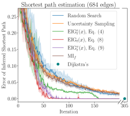
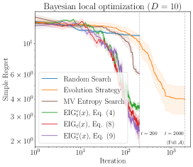
In Figure 6 we show the results of experiments where we compare the three estimators we proposed in Eqs. (4), (8), and (9), on shortest path estimation, Bayesian local optimization, and top-$k$ estimation. Each plot shows a measure of error on the $y$-axis, and number of iterations (i.e. queries) on the $x$-axis. In all three cases, we see that InfoBAX using $\operatorname{EIG}_{t}^{v}(x)$ and $\operatorname{EIG}_{t}(x)$ tend to perform best, followed closely by InfoBAX using $\operatorname{EIG}_{t}^{e}(x)$, and afterwards by the baseline methods. In the shortest path and top-$k$ estimation plots, we have also included an additional baseline, denoted $\text{MI}_{f}$, which sequentially chooses queries that maximize the expected information gain about the function $f$ (which has similarities with the UncertaintySampling baseline).

Details on estimating shortest paths

Here, we give details about our first experimental application, on estimating shortest paths in graphs (Section 4). Note that some examples of real-world networks with potentially expensive edge query lookups include transportation networks (e.g. querying or negotiating the price of transport, or assessing the cost of travel) (Bast et al., 2016), social networks (e.g. measuring the amount of social connection or targeted similar interests) (Backstrom and Leskovec, 2011; Pandey et al., 2019), and article networks (e.g. assessing the relevance of papers based on content) (Adafre and de Rijke, 2005; Neiswanger et al., 2014).

For the grid-shaped graph, to define edge costs, we use a rescaled Rosenbrock function (Rosenbrock, 1960) for $\mathcal{X}\subset\mathbb{R}^{2}$, defined as

$$f(x) =10^{-2}[((a-x_{2})^{2}+b(x_{2}-x_{1}^{2})^{2})]$$ (26)

with $a=1,b=100$ within the domain $-2\leq x_{1}\leq 2$, $-1\leq x_{2}\leq 4$. Each vertex within the grid is connected to its closest neighbors, corresponding to the ordinal and cardinal directions as shown in Figure 2.

We create our California graph from a subset of the graph network provided by Li et al. (2005), corresponding to the region within $36.7^{\circ}$N and $39.3^{\circ}$N and $122.5^{\circ}$W and $119.5^{\circ}$W. We use the vertex at $36.1494^{\circ}$N, $122.045158^{\circ}$W as our start vertex and the vertex at $38.913666^{\circ}$N, $120^{\circ}$W as our destination vertex. These two positions correspond to roughly Santa Cruz and Lake Tahoe, respectively. To obtain the ground truth edge cost function, we take the average of the cooridinates of the two vertices at each end of the edge and query its elevation from the OpenElevation dataset. To ensure that the edge costs are non-negative, we first rescale all edge costs by the max edge cost and add an offset of $0.1$ to each edge cost.

To ensure that our distribution $p(f)$ is supported on only non-negative functions, we transform the edge costs through the inverse of the softplus function and fit our Gaussian process on these transformed edge costs which can take on negative values. In all cases, when running InfoBAX , we draw $20$ posterior samples of the shortest path. We found that drawing more samples did not speed up convergence to the true shortest path.

We compute the $\operatorname{EIG}_{t}^{v}(x)$ acquisition function in Eq. (9), with respect to an execution path subsequence. In this case, the algorithm output is a sequence of edges and their respective edge costs, where each edge is associated with a point in $\mathcal{X}$, i.e. the average position between the two vertex positions. We therefore use the costs of the edges along a shortest path sample output as a $\widetilde{v}_{\mathcal{A}}$ in this acquisition function.

To evaluate the quality of each inferred shortest path, we use the 2D polygonal area between the inferred path and the truth shortest path. To do this, we decompose the area into a set of disjoint 2D polygons, and compute the area of each polygon using the shoelace algorithm (i.e. Gauss’s area formula).

Details on Bayesian local optimization

Here, we give details about our second experimental application, on Bayesian local optimization (Section 4). In this application, we demonstrate the use of InfoBAX for the task of black-box optimization, where the algorithm $\mathcal{A}$ is a local optimization algorithm—i.e. an algorithm consisting (typically) of an iterative procedure that returns some local optima with respect to a given initialization. Intuitively, the goal is to perform black-box optimization by choosing a sequence of function evaluations which efficiently yield a good estimate of the output of $\mathcal{A}$ (rather than, for example, choosing evaluations to directly infer a global optima of the function).

For our local optimization algorithm $\mathcal{A}$, we use a mutation-based evolution strategy. In this algorithm, we first initialize a population of $p$ vectors $V^{p}=\{v_{j}\}_{j=1}^{p}$ (where $v_{j}\in\mathcal{X}$) all to the same point, which is drawn uniformly at random from $\mathcal{X}$. The algorithm then proceeds over a sequence of $g$ generations. At each generation, we mutate each vector in this population via a normal proposal, i.e. draw $\widetilde{v}_{j}\sim\mathcal{N}(v_{j},\sigma_{pr}^{2})$ and set $v_{j}\leftarrow\widetilde{v}_{j}$, for all $v_{j}\in V^{p}$. We then query the function $f(v_{j})$, for each $v_{j}\in V^{p}$, and discard the bottom $(1-e)\%$ (where $e\in[0,1]$) of vectors in $V^{p}$ based on their function values, before proceeding on to the next generation. After $g$ generations, we return the vector $v_{j}^{*}$ that achieved the best queried function value over the course of the full algorithm (i.e. over all generations), and it’s observed function value $f(v_{j}^{*})$. We refer to this algorithm as EvolutionStrategy.

We show experimental results on minimization of three standard benchmark functions: Branin ($\mathcal{X}\subset\mathbb{R}^{2}$), Hartmann-6 ($\mathcal{X}\subset\mathbb{R}^{6}$), and Ackley-10 ($\mathcal{X}\subset\mathbb{R}^{10}$), defined as

$$\text{Branin:}\hskip 11.38109ptf(x) =\left(x_{2}-\frac{5.1}{(4\pi)^{2}}x_{1}^{2}+\frac{5}{\pi}x_{1}-6\right)^{2}+10\left(1-\frac{1}{8\pi}\right)\cos(x_{1})+10$$

$$\text{Hartmann-6:}\hskip 11.38109ptf(x) =-\sum_{i=1}^{4}\alpha_{i}\exp\left(-\sum_{j=1}^{6}A_{ij}(x_{j}-B_{ij})^{2}\right)$$

$$\text{Ackley-10:}\hskip 11.38109ptf(x) =-20\exp\left(-\frac{1}{5}\sqrt{\frac{1}{10}\sum_{i=1}^{10}x_{i}^{2}}\right)-\exp\left(\frac{1}{10}\sum_{i=1}^{10}\cos(2\pi x_{i})\right)+20+\exp(1),$$

where, in Hartmann-6,

$$\alpha =(1.0,1.2,3.0,3.2)^{\top}$$ (27)

$$A =\left(\begin{matrix}10&3&17&3.5&1.7&8\\ 0.05&10&17&0.1&8&14\\ 3&3.5&1.7&10&17&8\\ 17&8&0.05&10&0.1&14\end{matrix}\right)$$

$$B =\left(\begin{matrix}1312&1696&5569&124&8283&5886\\ 2329&4135&8307&3736&1004&9991\\ 2348&1451&3522&2883&3047&6650\\ 4047&8828&8732&5743&1091&381\end{matrix}\right)\times 10^{-4}.$$

We compare the performance of four methods: InfoBAX, RandomSearch (described in Section 4), EvolutionStategy, and MaxValueEntropySearch (Wang and Jegelka, 2017), which is a popular information-based Bayesian optimization method that aims to efficiently infer a global optima of $f$.

In InfoBAX, we draw 100 samples of $\widetilde{f}\sim p(f\>|\>\mathcal{D}_{t})$ and run $\mathcal{A}$ on these, in order to produce the execution path samples $\widetilde{e}_{\mathcal{A}}$. We then use the $\operatorname{EIG}_{t}^{v}(x)$ acquisition function from Eq. (9). Since the algorithm output consists of a vector $v_{j}^{*}\in\mathcal{X}$, and its value $f(v_{j}^{*})$, we use this tuple, $(v_{j}^{*},f(v_{j}^{*}))$, as the execution path subsequence in $\operatorname{EIG}_{t}^{v}(x)$. For acquisition optimization in both InfoBAX and MaxValueEntropySearch, we run a high-iteration random search algorithm. In MaxValueEntropySearch, for our global optimization procedure, we also run a high-iteration random search algorithm.

As an error metric, for each method we compute the Simple Regret, defined as the difference between the function value $f(\hat{x})$ at an estimated minimum $\hat{x}$ and the true minimal value $f(x^{*})$. For each method, we therefore need to produce an estimated minimum $\hat{x}$. For EvolutionStrategy, the estimated minimum is chosen to be the output of the algorithm (described above). For RandomSearch, the estimated minimum is chosen to be the input with lowest queried value, i.e. $\hat{x}:=\operatorname*{arg\,max}_{x\in\mathcal{D}_{t}}f(x)$. For both InfoBAX and MaxValueEntropySearch, the estimated minimum is chosen to be the estimated local or global optimum (respectively) of the GP posterior mean ${\mathbb{E}}_{p(f|\mathcal{D}_{t})}\left[f\right](x)=\mu_{T}(x)$.

References

- Adafre and de Rijke (2005) Sisay Fissaha Adafre and Maarten de Rijke. Discovering missing links in wikipedia. In Proceedings of the 3rd international workshop on Link discovery, pages 90–97, 2005.
- Back (1996) Thomas Back. Evolutionary algorithms in theory and practice: evolution strategies, evolutionary programming, genetic algorithms. Oxford university press, 1996.
- Backstrom and Leskovec (2011) Lars Backstrom and Jure Leskovec. Supervised random walks: predicting and recommending links in social networks. In Proceedings of the fourth ACM international conference on Web search and data mining, pages 635–644, 2011.
- Bast et al. (2016) Hannah Bast, Daniel Delling, Andrew Goldberg, Matthias Müller-Hannemann, Thomas Pajor, Peter Sanders, Dorothea Wagner, and Renato F Werneck. Route planning in transportation networks. In Algorithm engineering, pages 19–80. Springer, 2016.
- Beaumont (2010) Mark A Beaumont. Approximate bayesian computation in evolution and ecology. Annual review of ecology, evolution, and systematics, 41:379–406, 2010.
- Beaumont et al. (2002) Mark A Beaumont, Wenyang Zhang, and David J Balding. Approximate bayesian computation in population genetics. Genetics, 162(4):2025–2035, 2002.
- Bect et al. (2012) Julien Bect, David Ginsbourger, Ling Li, Victor Picheny, and Emmanuel Vazquez. Sequential design of computer experiments for the estimation of a probability of failure. Statistics and Computing, 22(3):773–793, 2012.
- Boecking et al. (2020) Benedikt Boecking, Willie Neiswanger, Eric Xing, and Artur Dubrawski. Interactive weak supervision: Learning useful heuristics for data labeling. arXiv preprint arXiv:2012.06046, 2020.
- Caselton and Zidek (1984) William F Caselton and James V Zidek. Optimal monitoring network designs. Statistics & Probability Letters, 2(4):223–227, 1984.
- Chaloner and Verdinelli (1995) Kathryn Chaloner and Isabella Verdinelli. Bayesian experimental design: A review. Stat. Sci., 10(3):273–304, 1995.
- Char et al. (2019) Ian Char, Youngseog Chung, Willie Neiswanger, Kirthevasan Kandasamy, Andrew O Nelson, Mark Boyer, Egemen Kolemen, and Jeff Schneider. Offline contextual bayesian optimization. Advances in Neural Information Processing Systems, 32:4627–4638, 2019.
- Chevalier et al. (2014) Clément Chevalier, Julien Bect, David Ginsbourger, Emmanuel Vazquez, Victor Picheny, and Yann Richet. Fast parallel kriging-based stepwise uncertainty reduction with application to the identification of an excursion set. Technometrics, 56(4):455–465, 2014.
- Csilléry et al. (2010) Katalin Csilléry, Michael GB Blum, Oscar E Gaggiotti, and Olivier François. Approximate bayesian computation (abc) in practice. Trends in ecology & evolution, 25(7):410–418, 2010.
- Davis and Rabinowitz (2007) Philip J Davis and Philip Rabinowitz. Methods of numerical integration. Courier Corporation, 2007.
- Dijkstra et al. (1959) Edsger W Dijkstra et al. A note on two problems in connexion with graphs. Numerische mathematik, 1(1):269–271, 1959.
- Drovandi and Pettitt (2013) Christopher C Drovandi and Anthony N Pettitt. Bayesian experimental design for models with intractable likelihoods. Biometrics, 69(4):937–948, 2013.
- Eriksson et al. (2019) David Eriksson, Michael Pearce, Jacob R Gardner, Ryan Turner, and Matthias Poloczek. Scalable global optimization via local bayesian optimization. arXiv preprint arXiv:1910.01739, 2019.
- Foster et al. (2019) Adam Foster, Martin Jankowiak, Eli Bingham, Paul Horsfall, Yee Whye Teh, Tom Rainforth, and Noah Goodman. Variational bayesian optimal experimental design. March 2019.
- Frazier (2018) Peter I Frazier. A tutorial on bayesian optimization. July 2018.
- Garnett et al. (2010) Roman Garnett, Michael A Osborne, and Stephen J Roberts. Bayesian optimization for sensor set selection. In Proceedings of the 9th ACM/IEEE international conference on information processing in sensor networks, pages 209–219, 2010.
- Garnett et al. (2012) Roman Garnett, Yamuna Krishnamurthy, Xuehan Xiong, Jeff Schneider, and Richard Mann. Bayesian optimal active search and surveying. arXiv preprint arXiv:1206.6406, 2012.
- Hennig and Schuler (2012) Philipp Hennig and Christian J Schuler. Entropy search for Information-Efficient global optimization. J. Mach. Learn. Res., 13(57):1809–1837, 2012.
- Hernández-Lobato et al. (2014) José Miguel Hernández-Lobato, Matthew W Hoffman, and Zoubin Ghahramani. Predictive entropy search for efficient global optimization of black-box functions. June 2014.
- Houlsby et al. (2012) Neil Houlsby, Ferenc Huszar, Zoubin Ghahramani, and Jose M Hernández-lobato. Collaborative gaussian processes for preference learning. In F Pereira, C J C Burges, L Bottou, and K Q Weinberger, editors, Advances in Neural Information Processing Systems 25, pages 2096–2104. Curran Associates, Inc., 2012.
- Kandasamy et al. (2019) Kirthevasan Kandasamy, Willie Neiswanger, Reed Zhang, Akshay Krishnamurthy, Jeff Schneider, and Barnabas Poczos. Myopic posterior sampling for adaptive goal oriented design of experiments. volume 97 of Proceedings of Machine Learning Research, pages 3222–3232, Long Beach, California, USA, 2019. PMLR.
- Kleinegesse and Gutmann (2019) Steven Kleinegesse and Michael U Gutmann. Efficient bayesian experimental design for implicit models. In Kamalika Chaudhuri and Masashi Sugiyama, editors, Proceedings of the Twenty Second International Conference on Artificial Intelligence and Statistics, volume 89 of Proceedings of Machine Learning Research, pages 476–485. PMLR, 2019.
- Kleinegesse et al. (2020) Steven Kleinegesse, Christopher Drovandi, and Michael U Gutmann. Sequential bayesian experimental design for implicit models via mutual information. March 2020.
- Krause et al. (2008) Andreas Krause, Ajit Singh, and Carlos Guestrin. Near-Optimal sensor placements in gaussian processes: Theory, efficient algorithms and empirical studies. J. Mach. Learn. Res., 9(8):235–284, 2008.
- Letham et al. (2020) Ben Letham, Roberto Calandra, Akshara Rai, and Eytan Bakshy. Re-examining linear embeddings for high-dimensional bayesian optimization. Advances in Neural Information Processing Systems, 33, 2020.
- Li et al. (2005) Feifei Li, Dihan Cheng, Marios Hadjieleftheriou, George Kollios, and Shang-Hua Teng. On trip planning queries in spatial databases. In International symposium on spatial and temporal databases, pages 273–290. Springer, 2005.
- Lindley (1956) Dennis V Lindley. On a measure of the information provided by an experiment. The Annals of Mathematical Statistics, pages 986–1005, 1956.
- Ma et al. (2014) Yifei Ma, Roman Garnett, and Jeff Schneider. Active area search via bayesian quadrature. In Artificial intelligence and statistics, pages 595–603. PMLR, 2014.
- Ma et al. (2015) Yifei Ma, Dougal Sutherland, Roman Garnett, and Jeff Schneider. Active pointillistic pattern search. In Artificial Intelligence and Statistics, pages 672–680. PMLR, 2015.
- Madsen (1973) Kaj Madsen. A root-finding algorithm based on newton’s method. BIT Numerical Mathematics, 13(1):71–75, 1973.
- Matthews et al. (2017) Alexander G de G Matthews, Mark Van Der Wilk, Tom Nickson, Keisuke Fujii, Alexis Boukouvalas, Pablo León-Villagrá, Zoubin Ghahramani, and James Hensman. Gpflow: A gaussian process library using tensorflow. J. Mach. Learn. Res., 18(40):1–6, 2017.
- Müller (2005) Peter Müller. Simulation based optimal design. In D K Dey and C R Rao, editors, Handbook of Statistics, volume 25, pages 509–518. Elsevier, January 2005.
- Neiswanger et al. (2014) Willie Neiswanger, Chong Wang, Qirong Ho, and Eric P Xing. Modeling citation networks using latent random offsets. In Proceedings of the Thirtieth Conference on Uncertainty in Artificial Intelligence, pages 633–642, 2014.
- Nelder and Mead (1965) John A Nelder and Roger Mead. A simplex method for function minimization. The computer journal, 7(4):308–313, 1965.
- Osborne et al. (2012) Michael Osborne, Roman Garnett, Zoubin Ghahramani, David K Duvenaud, Stephen J Roberts, and Carl E Rasmussen. Active learning of model evidence using bayesian quadrature. In Advances in neural information processing systems, pages 46–54, 2012.
- Pandey et al. (2019) Babita Pandey, Praveen Kumar Bhanodia, Aditya Khamparia, and Devendra Kumar Pandey. A comprehensive survey of edge prediction in social networks: Techniques, parameters and challenges. Expert Systems with Applications, 124:164–181, 2019.
- Pleiss et al. (2018) Geoff Pleiss, Jacob Gardner, Kilian Weinberger, and Andrew Gordon Wilson. Constant-time predictive distributions for gaussian processes. In International Conference on Machine Learning, pages 4114–4123. PMLR, 2018.
- Pleiss et al. (2020) Geoff Pleiss, Martin Jankowiak, David Eriksson, Anil Damle, and Jacob R. Gardner. Fast matrix square roots with applications to gaussian processes and bayesian optimization. In Hugo Larochelle, Marc’Aurelio Ranzato, Raia Hadsell, Maria-Florina Balcan, and Hsuan-Tien Lin, editors, Advances in Neural Information Processing Systems 33: Annual Conference on Neural Information Processing Systems 2020, NeurIPS 2020, December 6-12, 2020, virtual, 2020.
- Powell (1994) Michael JD Powell. A direct search optimization method that models the objective and constraint functions by linear interpolation. In Advances in optimization and numerical analysis, pages 51–67. Springer, 1994.
- Richardson (1911) Lewis Fry Richardson. Ix. the approximate arithmetical solution by finite differences of physical problems involving differential equations, with an application to the stresses in a masonry dam. Philosophical Transactions of the Royal Society of London. Series A, Containing Papers of a Mathematical or Physical Character, 210(459-470):307–357, 1911.
- Rios and Sahinidis (2013) Luis Miguel Rios and Nikolaos V Sahinidis. Derivative-free optimization: a review of algorithms and comparison of software implementations. Journal of Global Optimization, 56(3):1247–1293, 2013.
- Rosenbrock (1960) HoHo Rosenbrock. An automatic method for finding the greatest or least value of a function. The Computer Journal, 3(3):175–184, 1960.
- Rubin (1984) Donald B Rubin. Bayesianly justifiable and relevant frequency calculations for the applies statistician. The Annals of Statistics, pages 1151–1172, 1984.
- Seeger and Nickisch (2008) Matthias W Seeger and Hannes Nickisch. Large scale variational inference and experimental design for sparse generalized linear models. arXiv preprint arXiv:0810.0901, 2008.
- Shahriari et al. (2015) Bobak Shahriari, Kevin Swersky, Ziyu Wang, Ryan P Adams, and Nando De Freitas. Taking the human out of the loop: A review of bayesian optimization. Proceedings of the IEEE, 104(1):148–175, 2015.
- Spall et al. (1992) James C Spall et al. Multivariate stochastic approximation using a simultaneous perturbation gradient approximation. IEEE transactions on automatic control, 37(3):332–341, 1992.
- Tran et al. (2021) Kevin Tran, Willie Neiswanger, Kirby Broderick, Eric Xing, Jeff Schneider, and Zachary W Ulissi. Computational catalyst discovery: Active classification through myopic multiscale sampling. The Journal of Chemical Physics, 154(12):124118, 2021.
- Villemonteix et al. (2009) Julien Villemonteix, Emmanuel Vazquez, and Eric Walter. An informational approach to the global optimization of expensive-to-evaluate functions. Journal of Global Optimization, 44(4):509–534, 2009.
- Wang and Jegelka (2017) Zi Wang and Stefanie Jegelka. Max-value entropy search for efficient bayesian optimization. March 2017.
- Williams and Rasmussen (2006) Christopher KI Williams and Carl E Rasmussen. Gaussian processes for machine learning, volume 2. MIT press Cambridge, MA, 2006.
- Wilson et al. (2020) James Wilson, Viacheslav Borovitskiy, Alexander Terenin, Peter Mostowsky, and Marc Deisenroth. Efficiently sampling functions from gaussian process posteriors. In International Conference on Machine Learning, pages 10292–10302. PMLR, 2020.
- Zhong et al. (2020) Miao Zhong, Kevin Tran, Yimeng Min, Chuanhao Wang, Ziyun Wang, Cao-Thang Dinh, Phil De Luna, Zongqian Yu, Armin Sedighian Rasouli, Peter Brodersen, et al. Accelerated discovery of co 2 electrocatalysts using active machine learning. Nature, 581(7807):178–183, 2020.