Discrete-Time Fractional-Order Dynamical Networks Minimum-Energy State Estimation

Abstract

Fractional-order dynamical networks are increasingly being used to model and describe processes demonstrating long-term memory or complex interlaced dependencies amongst the spatial and temporal components of a wide variety of dynamical networks. Notable examples include networked control systems or neurophysiological networks which are created using electroencephalographic (EEG) or blood-oxygen-level-dependent (BOLD) data. As a result, the estimation of the states of fractional-order dynamical networks poses an important problem. To this effect, this paper addresses the problem of minimum-energy state estimation for discrete-time fractional-order dynamical networks (DT-FODN), where the state and output equations are affected by an additive noise that is considered to be deterministic, bounded, and unknown. Specifically, we derive the corresponding estimator and show that the resulting estimation error is exponentially input-to-state stable with respect to the disturbances and to a signal that is decreasing with the increase of the accuracy of the adopted approximation model. An illustrative example shows the effectiveness of the proposed method on real-world neurophysiological networks.

Biological Networks; Decision/Estimation Theory; Cyber-Physical Systems; Other Applications.

1 Introduction

In a wide variety of dynamical networks, it is often seen that a Markovian dependence of the current state on only the previous state is insufficient to describe the long-term behavior of the considered systems [1]. This is due to the fact that real-world networks often demonstrate behaviors in which the current system state is dependent on a combination of several past states or the entire gamut of states seen so far in time. Recent works suggest that discrete-time fractional-order dynamical networks (DT-FODN) evince great success in accurately modeling dynamics that show evidence of nonexponential power-law decay in the dependence of the current state on past states, systems exhibiting long-term memory or fractal properties, or dynamics where there are adaptations in multiple time scales [2, 3, 4, 5, 6]. These networks include biological swarms [7], networked control systems [8, 9, 10], and cyber-physical systems [11] to mention a few. Some of these relationships have also been explored in the context of neurophysiological networks constructed from electroencephalographic (EEG), electrocorticographic (ECoG), or blood-oxygen-level-dependent (BOLD) data [12, 13].

On the other hand, the problem of state estimation entails the retrieval of the internal state of a given network, often from incomplete or partial measurements of the network’s inputs and outputs. Solving this problem is of utmost importance, since, in the majority of real-world networks exchanging measurement information with each other, the network’s states are often not directly measurable, and a knowledge of the states is needed to, for example, collectively stabilize the system using state feedback. Given the fundamental nature of the problem, the existence of prior art in the context of state estimation of discrete-time fractional-order systems is no surprise [14, 15, 16, 17, 18, 19, 20].

Nonetheless, in practice, the assumptions in Kalman filter-like formulations are restrictive, as they assume white Gaussian additive process and measurement noises, which implies a uniform prevalence in the power spectrum. Due to this reason, we propose the design of a minimum-energy estimation framework for discrete-time fractional-order networks, where we assume that the state and output equations are affected by an additive disturbance and noise, respectively, that is considered to be deterministic, bounded, and unknown. First proposed by Mortensen [21], and later refined by Hijab [22], minimum-energy estimators produce an estimate of the system state that is the “most consistent” with the dynamics and the measurement updates of the system [23, 24, 25, 26, 27, 28, 29, 30, 31, 32, 33, 34, 35, 36, 37, 38].

In summary, the main contribution of this paper is a minimum-energy estimation procedure to estimate the states of a discrete-time fractional-order dynamical network (DT-FODN). In particular, we prove the exponential input-to-state stability of the estimation error when the aforementioned estimator is used to estimate the states of a DT-FODN. We also provide evidence of the efficacy of our approach via a pedagogical example showing the successful estimation of the states of a neurophysiological network constructed using EEG data.

Notation: The symbols $\mathbb{R},\mathbb{R}^{+},\mathbb{Z},\mathbb{N}$, and $\mathbb{N}^{+}$ denote, respectively, the set of reals, positive reals, integers, non-negative integers, and positive integers. Additionally, $\mathbb{R}^{n}$ and $\mathbb{R}^{n\times m}$ represent the set of column vectors of size $n$ and $n\times m$ matrices with real entries and $I$ denotes an identity matrix of appropriate order. For a given square matrix $M\in\mathbb{R}^{n\times n}$, the notation $M\succeq 0$ (respectively, $M\preceq 0$) indicates that the matrix $M$ is positive semidefinite (respectively, negative semidefinite), i.e., $v^{\mathsf{T}}Mv\geq 0$ (respectively, $v^{\mathsf{T}}Mv\leq 0$) for any $v\in\mathbb{R}^{n}$. Further, we use $M^{-\mathsf{T}}$ to denote the inverse of $M^{\mathsf{T}}$. We also write $A\succeq B$ and $A\preceq B$ to mean that the matrix $A-B$ is positive semidefinite and negative semidefinite, respectively. The Euclidean norm is denoted by $\|\cdot\|$.

2 Problem Formulation

In this section, we introduce DT-FODN and formulate the minimum-energy state estimation problem for DT-FODN.

2.1 Discrete-time fractional-order dynamical networks

Consider a left-bounded sequence $\{x[k]\}_{k\in\mathbb{Z}}$ over $k$, i.e., with $\limsup\limits_{k\to-\infty}\|x[k]\|<\infty$. Then, for any $\alpha\in\mathbb{R}^{+}$, the Grünwald-Letnikov fractional-order difference is defined as

$$\Delta^{\alpha}x[k]\coloneqq\sum_{j=0}^{\infty}c_{j}^{\alpha}x[k-j],\quad c_{j}^{\alpha}=(-1)^{j}\binom{\alpha}{j},$$ (1)

$$\quad\binom{\alpha}{j}=\begin{cases}1&\mbox{if }j=0,\\ \prod_{i=0}^{j-1}\frac{\alpha-i}{i+1}=\frac{\Gamma(\alpha+1)}{\Gamma(j+1)\Gamma(\alpha-j+1)}&\mbox{if }j>0,\end{cases}$$

for all $j\in\mathbb{N}$. The summation in (LABEL:eq:diff_op) is well-defined from the uniform boundedness of the sequence $\{x[k]\}_{k\in\mathbb{Z}}$ and the fact that $|c^{\alpha}_{j}|\leq\frac{\alpha^{j}}{j!}$, which implies that the sequence $\{c^{\alpha}_{j}\}_{j\in\mathbb{N}}$ is absolutely summable for any $\alpha\in\mathbb{R}^{+}$ [39, 40].

With the above ingredients, a discrete-time fractional-order dynamical network with additive disturbance can be described, respectively, by the state evolution and output equations

$$\sum_{i=1}^{l}A_{i}\Delta^{a_{i}}x[k+1]=\sum_{i=1}^{r}B_{i}\Delta^{b_{i}}u[k]+\sum_{i=1}^{s}G_{i}\Delta^{g_{i}}w[k],$$ (2a)

$$z[k]=C^{\prime}_{k}x[k]+v^{\prime}[k],$$ (2b)

with the variables $x[k]\in\mathbb{R}^{n}$, $u[k]\in\mathbb{R}^{m}$, and $w[k]\in\mathbb{R}^{p}$ denoting the state, input, and disturbance vectors at time step $k\in\mathbb{N}$, respectively. The scalars $a_{i}\in\mathbb{R}^{+}$ with $1\leq i\leq l$, $b_{i}\in\mathbb{R}^{+}$ with $1\leq i\leq r$, and $g_{i}\in\mathbb{R}^{+}$ with $1\leq i\leq s$ are the fractional-order coefficients corresponding, respectively, to the state, the input, and the disturbance. The vectors $z[k],v^{\prime}[k]\in\mathbb{R}^{q}$ denote, respectively, the output and measurement disturbance at time step $k\in\mathbb{N}$. We assume that the (unknown but deterministic) disturbance vectors are bounded as

$$\|w[k]\|\leq b_{w},\|v^{\prime}[k]\|\leq b_{v^{\prime}},\;k\in\mathbb{N},$$ (3)

for some scalars $b_{w},b_{v^{\prime}}\in\mathbb{R}^{+}$. We also assume that the control input $u[k]$ is known for all time steps $k\in\mathbb{N}$. We denote by $x[0]=x(0)$ the initial condition of the state at time $k=0$. In the computation of the fractional-order difference, we assume that the system is causal, i.e., the state, input, and disturbances are all considered to be zero before the initial time (i.e., $x[k]=0,u[k]=0$, and $w[k]=0$ for all $k<0$).

With the above ingredients, we seek to solve the following problem in this paper.

Problem 1.

Consider the quadratic weighted least-squares objective function

$$\mathcal{J}\left(x[0],\{w[i]\}_{i=0}^{N-1},\{v^{\prime}[j]\}_{j=1}^{N}\right)=\sum_{i=0}^{N-1}w[i]^{\mathsf{T}}Q_{i}^{-1}w[i]$$ (4)

$$+\sum_{j=1}^{N}v^{\prime}[j]^{\mathsf{T}}R_{j}^{-1}v^{\prime}[j]+(x[0]-\hat{x}_{0})^{\mathsf{T}}P_{0}^{-1}(x[0]-\hat{x}_{0}),$$

subject to the constraints

$$\sum_{i=1}^{l}A_{i}\Delta^{a_{i}}x[k+1]=\sum_{i=1}^{r}B_{i}\Delta^{b_{i}}u[k]+\sum_{i=1}^{s}G_{i}\Delta^{g_{i}}w[k]$$ (5a)

and

$$z[k]=C^{\prime}_{k}x[k]+v^{\prime}[k],$$ (5b)

for some $N\in\mathbb{N}$, with the weighting matrices $Q_{i}$ $(0\leq i\leq N-1),R_{j}$ $(1\leq j\leq N)$, and $P_{0}$ chosen to be symmetric and positive definite, and $\hat{x}_{0}$ chosen to be the a priori estimate of the system’s initial state. The minimum-energy estimation procedure seeks to solve the following optimization problem —l— { x[k] }k=0N, { w[i] }i=0N-1, { v’[j] }j=1NJ( x[0], { w[i] }_i=0^N-1, { v’[j] }_j=1^N ) (5a)   and   (5b), for some $N\in\mathbb{N}$.

Additionally, we consider the following mild technical assumption to hold.

Assumption 1.

The matrix $\sum_{i=1}^{l}A_{i}$ is invertible.

3 Minimum-Energy Estimation for Discrete-Time Fractional-Order Dynamical Networks

In order to derive the solution to Problem 1, we will first start with some alternative formulations of the DT-FODN and relevant definitions that will be used in the sequel. Then, we present the solution in Section 3.1 and in Section 3.2 we provide some additional properties of the derived solution, i.e., the exponential input-to-state stability of the estimation error. In Section 3.4, we present a practical discussion of the results obtained in the context of DT-FODN. All proofs are relegated to the appendix.

We start by considering a truncation of the last $\mathfrak{v}$ temporal components of (2a), which we will refer to as the $\mathfrak{v}$-approximation for the DT-FODN. That being said, we note that using Assumption 1, the DT-FODN model in (2a) can be equivalently written as

$$x[k+1]=\sum_{j=1}^{\infty}\check{A}_{j}x[k-j+1]+\sum_{j=0}^{\infty}\check{B}_{j}u[k-j]+\sum_{j=0}^{\infty}\check{G}_{j}w[k-j],$$ (6)

where $\check{A}_{j}=-\hat{A}_{0}^{-1}\hat{A}_{j}$, $\check{B}_{j}=\hat{A}_{0}^{-1}\hat{B}_{j}$, and $\check{G}_{j}=\hat{A}_{0}^{-1}\hat{G}_{j}$ with $\hat{A}_{j}=\sum_{i=1}^{l}A_{i}c_{j}^{a_{i}}$, $\hat{B}_{j}=\sum_{i=1}^{r}B_{i}c_{j}^{b_{i}}$, and $\hat{G}_{j}=\sum_{i=1}^{s}G_{i}c_{j}^{g_{i}}$. Furthermore, for any positive integer $\mathfrak{v}\in\mathbb{N}^{+}$, the DT-FODN model in (2a) can be recast as

$$\tilde{x}[k+1]=\tilde{A}_{\mathfrak{v}}\tilde{x}[k]+\tilde{B}_{\mathfrak{v}}u[k]+\tilde{G}_{\mathfrak{v}}r[k],\qquad\tilde{x}[0]=\tilde{x}_{0},$$ (7a)

$$y[k+1]=C_{k+1}\tilde{x}[k+1]+v[k+1],$$ (7b)

where

$$r[k]=\sum_{j={\mathfrak{v}}+1}^{\infty}\check{A}_{j}x[k-j+1]+\sum_{j={\mathfrak{v}}+1}^{\infty}\check{B}_{j}u[k-j]+\sum_{j=0}^{\infty}\check{G}_{j}w[k-j],$$ (8)

with the augmented state vector $\tilde{x}[k]=[x[k]^{\mathsf{T}},\ldots,x[k-\mathfrak{v}+1]^{\mathsf{T}},u[k-1]^{\mathsf{T}},\ldots,u[k-\mathfrak{v}]^{\mathsf{T}}]^{\mathsf{T}}\in\mathbb{R}^{\mathfrak{v}\times(n+m)}$ and appropriate matrices $\tilde{A}_{\mathfrak{v}},\tilde{B}_{\mathfrak{v}}$, and $\tilde{G}_{\mathfrak{v}}$, where $\tilde{x}_{0}=[x_{0}^{\mathsf{T}},0,\ldots,0]^{\mathsf{T}}$ denotes the initial condition. The matrices $\tilde{A}_{\mathfrak{v}}$ and $\tilde{B}_{\mathfrak{v}}$ are formed using the terms $\{\check{A}_{j}\}_{1\leq j\leq\mathfrak{v}}$ and $\{\check{B}_{j}\}_{1\leq j\leq\mathfrak{v}}$, while the remaining terms $\{\check{G}_{j}\}_{1\leq j<\infty}$ and the state and input components not included in $\tilde{x}[k]$ are absorbed into the term $\tilde{G}_{\mathfrak{v}}r[k]$. Furthermore, we refer to (7a) as the $\mathfrak{v}$-approximation of the DT-FODN presented in (2a).

3.1 Minimum-energy estimator

First, let us consider the quadratic weighted least-squares objective function

$$\mathcal{J}\left(\tilde{x}[0],\{r[i]\}_{i=0}^{N-1},\{v[j]\}_{j=1}^{N}\right)=\sum_{i=0}^{N-1}r[i]^{\mathsf{T}}Q_{i}^{-1}r[i]$$ (9)

$$+\sum_{j=1}^{N}v[j]^{\mathsf{T}}R_{j}^{-1}v[j]+(\tilde{x}[0]-\hat{x}_{0})^{\mathsf{T}}P_{0}^{-1}(\tilde{x}[0]-\hat{x}_{0}),$$

subject to the constraints

$$\begin{split}\bar{x}[k+1]&=\tilde{A}_{\mathfrak{v}}\bar{x}[k]+\tilde{B}_{\mathfrak{v}}u[k]+\tilde{G}_{\mathfrak{v}}\bar{r}[k],\end{split}$$ (10a)

$$\begin{split}y[k+1]&=C_{k+1}\bar{x}[k+1]+\bar{v}[k+1],\end{split}$$ (10b)

for some $N\in\mathbb{N}$. The weighting matrices $Q_{i}$ $(0\leq i\leq N-1)$ and $R_{j}$ $(1\leq j\leq N)$ are chosen to be symmetric and positive definite. The term $\hat{x}_{0}$ denotes the a priori estimate of the (unknown) initial state of the system, with the matrix $P_{0}$ being symmetric and positive definite.

Subsequently, to construct a minimum-energy estimator for the system (7), we then consider the weighted least-squares optimization problem —l— { ¯x[k] }k=0N, { ¯r[i] }i=0N-1, { ¯v[j] }j=1NJ( ~x[0], { r[i] }_i=0^N-1, { v[j] }_j=1^N ) (10a)   and   (10b), for some $N\in\mathbb{N}$. The following theorem then certifies the solution of the minimum-energy estimation problem posed in (3.1).

Theorem 1.

Denote by $\hat{x}[k]$ the state vector that corresponds to the solution of the optimization problem (3.1). Then, $\hat{x}[k]$ satisfies the recursion

$$\hat{x}[k+1]=\tilde{A}_{\mathfrak{v}}\hat{x}[k]+\tilde{B}_{\mathfrak{v}}u[k]+K_{k+1}\Big{(}y[k+1]$$ (11)

$$-C_{k+1}\Big{(}\tilde{A}_{\mathfrak{v}}\hat{x}[k]+\tilde{B}_{\mathfrak{v}}u[k]\Big{)}\Big{)},\quad 0\leq k\leq N-1,$$

with initial conditions specified for $\hat{x}_{0}$ and $\{u[j]\}_{j=0}^{k}$, and with the update equations

$$K_{k+1}=M_{k+1}C_{k+1}^{\mathsf{T}}(C_{k+1}M_{k+1}C_{k+1}^{\mathsf{T}}+R_{k+1})^{-1},$$ (12a)

$$M_{k+1}=\tilde{A}_{\mathfrak{v}}P_{k}\tilde{A}_{\mathfrak{v}}^{\mathsf{T}}+\tilde{G}_{\mathfrak{v}}Q_{k}\tilde{G}_{\mathfrak{v}}^{\mathsf{T}},$$ (12b)

and

$$P_{k+1}=(I-K_{k+1}C_{k+1})M_{k+1}(I-K_{k+1}C_{k+1})^{\mathsf{T}}$$ (12c)

$$+K_{k+1}R_{k+1}K_{k+1}^{\mathsf{T}}=(I-K_{k+1}C_{k+1})M_{k+1},$$

with symmetric and positive definite $P_{0}$.

In Theorem 1, the dynamics of the recursion in (11) (with the initial conditions on $\hat{x}_{0}$ and the values of $\{u[j]\}_{j=0}^{k}$ being known) along with the update equations (12) together solve Problem 1 completely. It is interesting to note here that the output term $y[k+1]$ presented in (10b) and (11) is the output of the $\mathfrak{v}$-approximated system (7), which, in turn, is simply a subset of the outputs $z[k+1]$ obtained from (2b), truncated $\mathfrak{v}$ time steps in the past, provided $v[k]$ and $C_{k}$ are formed from the appropriate blocks of $v^{\prime}[k]$ and $C^{\prime}_{k}$ for all $k\in\mathbb{N}$.

In what follows, we show that given the $\mathfrak{v}$-approximation outlined in (7a), the evolution of the Lyapunov equation admits a solution over time, by establishing the exponential input-to-state stability of the estimation error.

3.2 Exponential input-to-state stability of the estimation error

In order to prove the exponential input-to-state stability of the minimum-energy estimation error, we need to consider the following mild technical assumptions.

Assumption 2.

There exist constants $\underline{\alpha},\overline{\alpha},\beta,\gamma\in\mathbb{R}^{+}$ such that

$$\underline{\alpha}I\preceq\tilde{A}_{\mathfrak{v}}\tilde{A}_{\mathfrak{v}}^{\mathsf{T}}\preceq\overline{\alpha}I,\quad\tilde{G}_{\mathfrak{v}}\tilde{G}_{\mathfrak{v}}^{\mathsf{T}}\preceq\beta I,\>\>\text{and}\quad C_{k}^{\mathsf{T}}C_{k}\preceq\gamma I,$$ (13)

for all $k\in\mathbb{N}$.

First, notice that the state transition matrix for the dynamics in (7a) is given by

$$\Phi(k,k_{0})=\tilde{A}_{\mathfrak{v}}^{(k-k_{0})},\quad\text{with}\quad\Phi(k_{0},k_{0})=I,$$ (14)

for all $k\geq k_{0}\geq 0$. We also consider the discrete-time controllability Gramian associated with the dynamics (7a) described by

$$W_{c}(k,k_{0})=\sum_{i=k_{0}}^{k-1}\Phi(k,i+1)\tilde{G}_{\mathfrak{v}}\tilde{G}_{\mathfrak{v}}^{\mathsf{T}}\Phi^{\mathsf{T}}(k,i+1),$$ (15)

and the discrete-time observability Gramian associated with (7a) to be

$$W_{o}(k,k_{0})=\sum_{i=k_{0}+1}^{k}\Phi^{\mathsf{T}}(i,k_{0})C_{i}^{\mathsf{T}}C_{i}\Phi(i,k_{0}),$$ (16)

for $k\geq k_{0}\geq 0$. We also make the following assumptions regarding complete uniform controllability and complete uniform observability of the $\mathfrak{v}$-approximated system in (7a).

Assumption 3.

The $\mathfrak{v}$-approximated system (7a) is completely uniformly controllable, i.e., there exist constants $\delta\in\mathbb{R}^{+}$ and $N_{c}\in\mathbb{N}^{+}$ such that

$$W_{c}(k+N_{c},k)\succeq\delta I,$$ (17)

for all $k\geq 0$.

Assumption 4.

The $\mathfrak{v}$-approximated system (7a) is completely uniformly observable, i.e., there exist constants $\varepsilon\in\mathbb{R}^{+}$ and $N_{o}\in\mathbb{N}^{+}$ such that

$$W_{o}(k+N_{o},k)\succeq\varepsilon\Phi^{\mathsf{T}}(k+N_{o},k)\Phi(k+N_{o},k),$$ (18)

for all $k\geq 0$.

Next, we also present an assumption certifying lower and upper bounds on the weight matrices $Q_{k}$ and $R_{k+1}$ in (9).

Assumption 5.

Without loss of generality, we assume that the weight matrices $Q_{k}$ and $R_{k+1}$ satisfy

$$\underline{\vartheta}I\preceq Q_{k}\preceq\overline{\vartheta}I\quad\text{and}\quad\underline{\rho}I\preceq R_{k+1}\preceq\overline{\rho}I,$$ (19)

for all $k\geq 0$ and constants $\underline{\vartheta},\overline{\vartheta},\underline{\rho},\overline{\rho}\in\mathbb{R}^{+}$.

3.2.1 Bounds on the covariance matrix $P_{k}$

In this section, we establish lower and upper bounds for the matrix $P_{k}$, which will be required in Section 3.2.2, where we use an approach using Lyapunov functions in order to show that the estimation error is exponentially input-to-state stable.

Lemma 1.

Given Assumptions 2 and 3 and the constant $\underline{\pi}\in\mathbb{R}^{+}$, we have that

$$P_{k}\succeq\underline{\pi}(N_{c})I$$ (20)

holds for all $k\geq N_{c}$.

Lemma 2.

Given Assumptions 2 and 4 and the constant $\overline{\pi}\in\mathbb{R}^{+}$, we have that

$$P_{k}\preceq\overline{\pi}(N_{o})I$$ (21)

holds for all $k\geq N_{o}$.

3.2.2 Exponential input-to-state stability of the estimation error

We start with the minimum-energy estimation error $e[k]$, given by

$$e[k]=\hat{x}[k]-\tilde{x}[k].$$ (22)

Next, we certify that the estimation error associated with the minimum-energy estimation process is exponentially input-to-state stable.

Theorem 2.

Under Assumptions 2, 3, and 4, there exist constants $\sigma,\tau,\chi,\psi\in\mathbb{R}^{+}$ with $\tau<1$ such that the estimation error $e[k]$ satisfies

$$\|e[k]\| \leq\max\Bigg{\{}\sigma\tau^{k-k_{0}}\|e[k_{0}]\|,\>\chi\max_{k_{o}\leq i\leq k-1}\|r[i]\|,$$ (23)

$$\psi\max_{k_{o}\leq j\leq k-1}\|v[j+1]\|\Bigg{\}}$$

for all $k\geq k_{0}\geq\max\{N_{c},N_{o}\}$.

3.3 Discussion

It is interesting to note that the bound on the estimation error $e[k]$ in (23) actually depends on $\|r[i]\|$, where $k_{0}\leq i\leq k-1$ for all $i\in\mathbb{N}$. In fact, a distinguishing feature of DT-FODN is the presence of a finite non-zero disturbance term in the input-to-state stability bound of the tracking error when tracking a state other than the origin. This disturbance is dependent on the upper bounds on the non-zero reference state being tracked as well as the input. While the linearity of the Grünwald-Letnikov fractional-order difference operator allows one to mitigate this issue in the case of tracking a non-zero exogenous state by a suitable change of state and input coordinates, this approach is not one we can pursue in this paper, since the state we wish to estimate is unknown. However, it can be shown that as the value of $\mathfrak{v}$ in the $\mathfrak{v}$-approximation increases, the upper bound associated with $\|r[i]\|$ decreases drastically since the $\mathfrak{v}$-approximation gives us progressively better representations of the unapproximated system. This further implies that $\|r[i]\|$ in (23) stays bounded, with progressively smaller upper bounds associated with $\|r[i]\|$ (and hence, $\|e[k]\|$) with increasing $\mathfrak{v}$.

Lastly, the estimation error associated with the minimum-energy estimation process in (22) is defined in terms of the state of the $\mathfrak{v}$-approximated system $\tilde{x}[k]$. In reality, as detailed above, with larger values of $\mathfrak{v}$, the $\mathfrak{v}$-approximated system approaches the real network dynamics, and thus we obtain an expression for the estimation error with respect to the real system in the limiting case, where the input-to-state stability bound presented in Theorem 2 holds.

3.4 Illustrative Example

In this section, we consider the performance of the minimum-energy estimation paradigm on real-world neurophysiological networks considering EEG data. Specifically, we use $150$ noisy measurements taken from $4$ channels of a $64$-channel EEG signal which records the brain activity of subjects, as shown in Figure 1. The subjects were asked to perform a variety of motor and imagery tasks, and the specific choice of the $4$ channels was dictated due to them being positioned over the motor cortex of the brain, and, therefore, enabling us to predict motor actions such as the movement of the hands and feet. The data was collected using the BCI$2000$ system with a sampling rate of $160$ Hz [41, 42]. The spatial and temporal parameter components of the DT-FODN assumed to model the original EEG data were identified using the methods described in [43]. The matrices $B_{i}=\begin{bmatrix}1&1&1&1\end{bmatrix}^{\mathsf{T}}$ for all $i$.

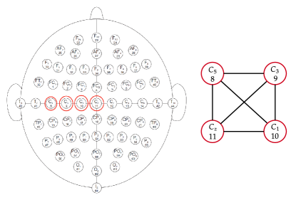
Figure 1: The distribution of the sensors for the measurement of EEG data is shown on the left. The channel labels are shown along with their corresponding numbers and the selected channels over the motor cortex are shown in red. The corresponding network formed by the EEG sensors is shown on the right.

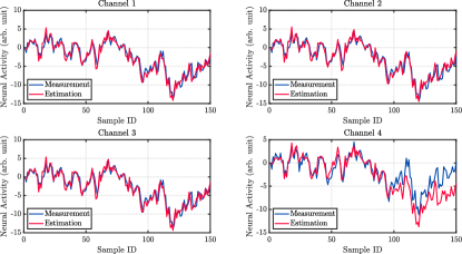
Figure 2: Comparison between the measured output of the $\mathfrak{v}$-augmented system (with $\mathfrak{v}=2$) versus the estimated output of a minimum-energy estimator implemented on the same, in the presence of process and measurement noises for $4$ channels of a $64$-channel EEG signal.

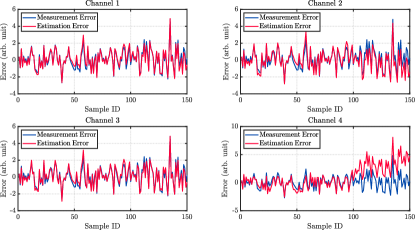
Figure 3: Comparison between the measurement error of the $\mathfrak{v}$-augmented system (with $\mathfrak{v}=2$) versus the estimation error of a minimum-energy estimator implemented on the same, in the presence of process and measurement noises for $4$ channels of a $64$-channel EEG signal.

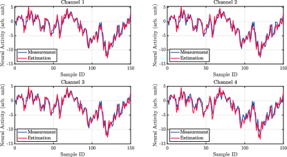
Figure 4: Comparison between the measured output of the $\mathfrak{v}$-augmented system (with $\mathfrak{v}=10$) versus the estimated output of a minimum-energy estimator implemented on the same, in the presence of process and measurement noises for $4$ channels of a $64$-channel EEG signal.

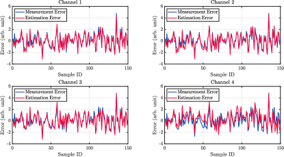
Figure 5: Comparison between the measurement error of the $\mathfrak{v}$-augmented system (with $\mathfrak{v}=10$) versus the estimation error of a minimum-energy estimator implemented on the same, in the presence of process and measurement noises for $4$ channels of a $64$-channel EEG signal.

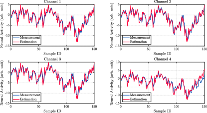
Figure 6: Comparison between the measured output of the $\mathfrak{v}$-augmented system (with $\mathfrak{v}=20$) versus the estimated output of a minimum-energy estimator implemented on the same, in the presence of process and measurement noises for $4$ channels of a $64$-channel EEG signal.

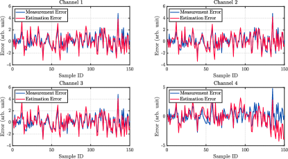
Figure 7: Comparison between the measurement error of the $\mathfrak{v}$-augmented system (with $\mathfrak{v}=20$) versus the estimation error of a minimum-energy estimator implemented on the same, in the presence of process and measurement noises for $4$ channels of a $64$-channel EEG signal.

The results of our approach, considering different values of $\mathfrak{v}$, are shown in Figures 2 and 3 (for $\mathfrak{v}=2$), Figures 4 and 5 (for $\mathfrak{v}=10$), and Figures 6 and 7 (for $\mathfrak{v}=20$), which show, respectively (for each value of $\mathfrak{v}$), the comparison between the measured output of the network with noise and the estimated response obtained from the minimum-energy estimator, and also the juxtaposition of the measurement error and the estimation error of the minimum-energy estimation process. We find that the minimum-energy estimator is successfully able to estimate the states in the presence of noise in both the dynamics and the measurement processes.

We also note from the Figures 2 and 3 that when $\mathfrak{v}=2$, we get comparatively larger estimation errors associated with the last $50$ or so samples of Channel $4$, and that this behavior can be mitigated by increasing the value of $\mathfrak{v}$, e.g., by choosing $\mathfrak{v}=10$ or $\mathfrak{v}=20$. This is in line with the discussion in Section 3.3, and choosing a larger value of $\mathfrak{v}$ can always, in practice, provide us with better estimation performances, as seen from this example.

4 Conclusion

In this paper, we introduced minimum-energy state estimation for discrete-time fractional-order dynamical networks. In particular, the aforementioned minimum-energy estimator is capable of providing an estimate of the unknown states of a discrete-time fractional-order dynamical network while assuming that the associated process and measurement noises are deterministic, bounded, and unknown in nature. We proved that the minimum-energy estimation error is exponentially input-to-state stable and illustrated its performance on real-world neurophysiological EEG networks. Future work will focus on the construction of a resilient and attack-resistant version of the minimum-energy estimator, to take into consideration adversarial attacks or artifacts associated with the measurement process, since the former approach is consistent with the fact that adversarial attacks on sensors often do not follow any particular dynamical or stochastic characterization.

Proof of Theorem 1: We first consider a single-stage state transition of the system in (10) and then, sequentially, course through the remaining state transitions. Then, the recursions in (11) and (12) are obtained using the principle of feedback invariance [44] and the minimum-energy estimator for discrete-time LTI systems [25], since the $\mathfrak{v}$-approximated DT-FODN in (7a) fits the latter description. ∎

Proof of Lemma 1: Suppose $L_{k+1}$ is an arbitrary matrix. We can write

$$(P_{k+1}+L_{k+1}L_{k+1}^{\mathsf{T}})^{-1} =\big{(}(M_{k+1}^{-1}+C_{k+1}^{\mathsf{T}}R_{k+1}^{-1}C_{k+1})^{-1}$$ (24)

$$+L_{k+1}L_{k+1}^{\mathsf{T}}\big{)}^{-1},$$

where we use the equation

$$P_{k+1}^{-1}=M_{k+1}^{-1}+C_{k+1}^{\mathsf{T}}R_{k+1}^{-1}C_{k+1},$$ (25)

which can be obtained from (12c) using the Woodbury identity [45, eq. (157)]. Notice that the invertibility of $P_{k}$ and $M_{k+1}$ for any $k\geq 0$ is a consequence of (12), Assumptions 2 and 5, and the fact that $P_{0}$ is positive definite.

Subsequently, using the bounds in Assumptions 2 and 5, and defining $\beta_{1}=\frac{\gamma}{\underline{\rho}}$, we have

$$\left(\mathnormal{P}_{k+1}+\mathnormal{L}_{k+1}\mathnormal{L}_{k+1}^{\mathsf{T}}\right)^{-1}$$

$$\preceq\left(\left(\mathnormal{M}_{k+1}^{-1}+\beta_{1}\mathnormal{I}\right)^{-1}+\mathnormal{L}_{k+1}\mathnormal{L}_{k+1}^{\mathsf{T}}\right)^{-1}$$

$$\stackrel{{\scriptstyle(\dagger)}}{{=}}\left(\frac{1}{\beta_{1}}\mathnormal{I}-\frac{1}{\beta_{1}^{2}}\left(\mathnormal{M}_{k+1}+\frac{1}{\beta_{1}}\mathnormal{I}\right)^{-1}+\mathnormal{L}_{k+1}\mathnormal{L}_{k+1}^{\mathsf{T}}\right)^{-1}$$

$$\stackrel{{\scriptstyle(\ddagger)}}{{=}}\frac{1}{\beta_{1}^{2}}\left(\frac{1}{\beta_{1}}\mathnormal{I}+\mathnormal{L}_{k+1}\mathnormal{L}_{k+1}^{\mathsf{T}}\right)^{-1}$$

$$\times\left(\mathnormal{M}_{k+1}+\frac{1}{\beta_{1}}\mathnormal{I}-\frac{1}{\beta_{1}^{2}}\left(\frac{1}{\beta_{1}}\mathnormal{I}+\mathnormal{L}_{k+1}\mathnormal{L}_{k+1}^{\mathsf{T}}\right)^{-1}\right)^{-1}$$

$$\times\left(\frac{1}{\beta_{1}}\mathnormal{I}+\mathnormal{L}_{k+1}\mathnormal{L}_{k+1}^{\mathsf{T}}\right)^{-1}+\left(\frac{1}{\beta_{1}}\mathnormal{I}+\mathnormal{L}_{k+1}\mathnormal{L}_{k+1}^{\mathsf{T}}\right)^{-1}$$

$$\stackrel{{\scriptstyle(\diamond)}}{{=}}\frac{1}{\beta_{1}^{2}}\left(\beta_{1}\mathnormal{I}-\beta_{1}^{2}\mathnormal{L}_{k+1}\left(\mathnormal{I}+\beta_{1}\mathnormal{L}_{k+1}^{\mathsf{T}}\mathnormal{L}_{k+1}\right)^{-1}\mathnormal{L}_{k+1}^{\mathsf{T}}\right)$$

$$\times\left(\mathnormal{M}_{k+1}+\mathnormal{L}_{k+1}\left(\mathnormal{I}+\beta_{1}\mathnormal{L}_{k+1}^{\mathsf{T}}\mathnormal{L}_{k+1}\right)^{-1}\mathnormal{L}_{k+1}^{\mathsf{T}}\right)^{-1}$$

$$\times\left(\beta_{1}\mathnormal{I}-\beta_{1}^{2}\mathnormal{L}_{k+1}\left(\mathnormal{I}+\beta_{1}\mathnormal{L}_{k+1}^{\mathsf{T}}\mathnormal{L}_{k+1}\right)^{-1}\mathnormal{L}_{k+1}^{\mathsf{T}}\right)+\beta_{1}\mathnormal{I}$$

$$-\beta_{1}^{2}\mathnormal{L}_{k+1}\left(\mathnormal{I}+\beta_{1}\mathnormal{L}_{k+1}^{\mathsf{T}}\mathnormal{L}_{k+1}\right)^{-1}\mathnormal{L}_{k+1}^{\mathsf{T}}$$

$$\stackrel{{\scriptstyle(\blackdiamond)}}{{\preceq}}2\beta_{1}^{2}\mathnormal{L}_{k+1}\left(\mathnormal{I}+\beta_{1}\mathnormal{L}_{k+1}^{\mathsf{T}}\mathnormal{L}_{k+1}\right)^{-1}\mathnormal{L}_{k+1}^{\mathsf{T}}$$

$$\times\left(\mathnormal{M}_{k+1}+\mathnormal{L}_{k+1}\left(\mathnormal{I}+\beta_{1}\mathnormal{L}_{k+1}^{\mathsf{T}}\mathnormal{L}_{k+1}\right)^{-1}\mathnormal{L}_{k+1}^{\mathsf{T}}\right)^{-1}$$

$$\times\mathnormal{L}_{k+1}\left(\mathnormal{I}+\beta_{1}\mathnormal{L}_{k+1}^{\mathsf{T}}\mathnormal{L}_{k+1}\right)^{-1}\mathnormal{L}_{k+1}^{\mathsf{T}}$$

$$+2\left(\mathnormal{M}_{k+1}+\mathnormal{L}_{k+1}\left(\mathnormal{I}+\beta_{1}\mathnormal{L}_{k+1}^{\mathsf{T}}\mathnormal{L}_{k+1}\right)^{-1}\mathnormal{L}_{k+1}^{\mathsf{T}}\right)^{-1}$$

$$+\beta_{1}\mathnormal{I}-\beta_{1}^{2}\mathnormal{L}_{k+1}\left(\mathnormal{I}+\beta_{1}\mathnormal{L}_{k+1}^{\mathsf{T}}\mathnormal{L}_{k+1}\right)^{-1}\mathnormal{L}_{k+1}^{\mathsf{T}}$$

$$\preceq 2(M_{k+1}+\alpha_{1,k+1}L_{k+1}L_{k+1}^{\mathsf{T}})^{-1}+2\beta_{1}I,$$ (26)

where $\alpha_{1,k+1}=\|I+\beta_{1}L_{k+1}^{\mathsf{T}}L_{k+1}\|^{-1}$. The equalities $(\dagger)$, $(\ddagger)$, and $(\diamond)$ in (4) are obtained via three successive applications of the Woodbury identity and the inequality $(\blackdiamond)$ in (4) is obtained by using the Young-like inequality

$$(f(v)+g(v))^{\mathsf{T}}(f(v)+g(v))\leq 2f^{\mathsf{T}}(v)g(v)+2g^{\mathsf{T}}(v)f(v),$$ (27)

with $f(v)=(M_{k+1}+L_{k+1}(I+\beta_{1}L_{k+1}^{\mathsf{T}}L_{k+1})^{-1}L_{k+1}^{\mathsf{T}})^{-\frac{1}{2}}v$ and $g(v)=-\beta_{1}(M_{k+1}+L_{k+1}(I+\beta_{1}L_{k+1}^{\mathsf{T}}L_{k+1})^{-1}L_{k+1}^{\mathsf{T}})^{-\frac{1}{2}}L_{k+1}(I+\beta_{1}L_{k+1}^{\mathsf{T}}L_{k+1})^{-1}L_{k+1}^{\mathsf{T}}v$.

Plugging in the value of $M_{k+1}$ from the update equations (12), we have

$$(\mathnormal{P}_{k+1}+\mathnormal{L}_{k+1}\mathnormal{L}_{k+1}^{\mathsf{T}})^{-1}\preceq 2\beta_{1}I+2\tilde{A}_{\mathfrak{v}}^{-\mathsf{T}}$$ (28)

$$\times \left(P_{k}+\tilde{A}_{\mathfrak{v}}^{-1}(\tilde{G}_{\mathfrak{v}}Q_{k}\tilde{G}_{\mathfrak{v}}^{\mathsf{T}}+\alpha_{1,k+1}L_{k+1}L_{k+1}^{\mathsf{T}})\tilde{A}_{\mathfrak{v}}^{-\mathsf{T}}\right)^{-1}\tilde{A}_{\mathfrak{v}}^{-1}.$$

Now, for any $k\geq 0$, define recursively

$$L_{j}L_{j}^{\mathsf{T}}=\tilde{A}_{\mathfrak{v}}^{-1}(\tilde{G}_{\mathfrak{v}}Q_{j}\tilde{G}_{\mathfrak{v}}^{\mathsf{T}}+\alpha_{1,j+1}L_{j+1}L_{j+1}^{\mathsf{T}})\tilde{A}_{\mathfrak{v}}^{-\mathsf{T}}$$ (29)

for $k\leq j\leq k+N_{c}-1$, with $L_{k+N_{c}}L_{k+N_{c}}^{\mathsf{T}}=0$. By substituting (29) into (28), and repeatedly applying the resulting inequality we obtain

$$\mathnormal{P}_{k+N_{c}}^{-1}\preceq 2^{N_{c}}\Phi^{-\mathsf{T}}\left(k+N_{c},k\right)\left(\mathnormal{P}_{k}+\mathnormal{L}_{k}\mathnormal{L}_{k}^{\mathsf{T}}\right)^{-1}$$ (30)

$$\times\Phi^{-1}\left(k+N_{c},k\right)+2\beta_{1}\sum_{i=0}^{N_{c}-1}2^{i}$$

$$\times\Phi^{-\mathsf{T}}\left(k+N_{c},k+N_{c}-i\right)\Phi^{-1}\left(k+N_{c},k+N_{c}-i\right).$$

Using the bounds defined in Assumption 5, (15), and (29), we can write

$$L_{k}L_{k}^{\mathsf{T}}\succeq\gamma_{1}\Phi^{-1}(k+N_{c},k)W_{c}(k+N_{c},k)\Phi^{-\mathsf{T}}(k+N_{c},k),$$ (31)

with $\gamma_{1}=\underline{\vartheta}\prod_{j=k}^{k+N_{c}-1}\alpha_{1,j+1}$. Aggregating the bounds in (30), (31), and invoking Assumptions 2 and 3, we have

$$P_{k+N_{c}}\succeq\underbrace{\left(\frac{2^{N_{c}}}{\gamma_{1}\delta}+2\beta_{1}\sum_{i=0}^{N_{c}-1}\left(\frac{2}{\underline{\alpha}}\right)^{i}\right)^{-1}}_{\underline{\pi}(N_{c})}I.$$ (32)

∎

Proof of Lemma 2: Suppose $Y_{k+1}$ is an arbitrary matrix. We can write

$$(P_{k+1}^{-1}+Y_{k+1}^{\mathsf{T}}Y_{k+1})^{-1} =\Big{(}(\tilde{A}_{\mathfrak{v}}P_{k}\tilde{A}_{\mathfrak{v}}^{\mathsf{T}}+\tilde{G}_{\mathfrak{v}}Q_{k}\tilde{G}_{\mathfrak{v}}^{\mathsf{T}})^{-1}$$ (33)

$$+Z_{k+1}^{\mathsf{T}}Z_{k+1}\Big{)}^{-1},$$

where the matrix $Z_{k+1}$ is defined as

$$Z_{k+1}=C_{k+1}^{\mathsf{T}}R_{k+1}^{-1}C_{k+1}+Y^{\mathsf{T}}_{k+1}Y_{k+1}.$$ (34)

Using the bounds in Assumptions 2 and 5, and defining $\beta_{2}=\beta\overline{\vartheta}$, we have

$$\left(\mathnormal{P}_{k+1}^{-1}+\mathnormal{Y}_{k+1}^{\mathsf{T}}\mathnormal{Y}_{k+1}\right)^{-1}$$

$$\preceq\left(\left(\tilde{A}_{\mathfrak{v}}\mathnormal{P}_{k}\tilde{A}_{\mathfrak{v}}^{\mathsf{T}}+\beta_{2}\mathnormal{I}\right)^{-1}+\mathnormal{Z}_{k+1}^{\mathsf{T}}\mathnormal{Z}_{k+1}\right)^{-1}$$

$$\stackrel{{\scriptstyle(\bigtriangleup)}}{{=}}\Bigg{(}\frac{1}{\beta_{2}}\mathnormal{I}-\frac{1}{\beta_{2}^{2}}\tilde{A}_{\mathfrak{v}}\left(\mathnormal{P}_{k}^{-1}+\frac{1}{\beta_{2}}\tilde{A}_{\mathfrak{v}}^{\mathsf{T}}\tilde{A}_{\mathfrak{v}}\right)^{-1}\tilde{A}_{\mathfrak{v}}^{\mathsf{T}}$$

$$+\mathnormal{Z}_{k+1}^{\mathsf{T}}\mathnormal{Z}_{k+1}\Bigg{)}^{-1}$$

$$\stackrel{{\scriptstyle(\bigtriangledown)}}{{=}}\frac{1}{\beta_{2}^{2}}\left(\frac{1}{\beta_{2}}\mathnormal{I}+\mathnormal{Z}_{k+1}^{\mathsf{T}}\mathnormal{Z}_{k+1}\right)^{-1}\tilde{A}_{\mathfrak{v}}$$

$$\times\left(\mathnormal{P}_{k}^{-1}+\frac{1}{\beta_{2}}\tilde{A}_{\mathfrak{v}}^{\mathsf{T}}\tilde{A}_{\mathfrak{v}}-\frac{1}{\beta_{2}^{2}}\tilde{A}_{\mathfrak{v}}^{\mathsf{T}}\left(\frac{1}{\beta_{2}}\mathnormal{I}+\mathnormal{Z}_{k+1}^{\mathsf{T}}\mathnormal{Z}_{k+1}\right)^{-1}\tilde{A}_{\mathfrak{v}}\right)^{-1}$$

$$\times\tilde{A}_{\mathfrak{v}}^{\mathsf{T}}\left(\frac{1}{\beta_{2}}\mathnormal{I}+\mathnormal{Z}_{k+1}^{\mathsf{T}}\mathnormal{Z}_{k+1}\right)^{-1}+\left(\frac{1}{\beta_{2}}\mathnormal{I}+\mathnormal{Z}_{k+1}^{\mathsf{T}}\mathnormal{Z}_{k+1}\right)^{-1}$$

$$\stackrel{{\scriptstyle(\centerdot)}}{{=}}\frac{1}{\beta_{2}^{2}}\left(\beta_{2}\mathnormal{I}-\beta_{2}^{2}\mathnormal{Z}_{k+1}^{\mathsf{T}}\left(\mathnormal{I}+\beta_{2}\mathnormal{Z}_{k+1}\mathnormal{Z}_{k+1}^{\mathsf{T}}\right)^{-1}\mathnormal{Z}_{k+1}\right)\tilde{A}_{\mathfrak{v}}$$

$$\times\left(\mathnormal{P}_{k}^{-1}+\tilde{A}_{\mathfrak{v}}^{\mathsf{T}}\mathnormal{Z}_{k+1}^{\mathsf{T}}\left(\mathnormal{I}+\beta_{2}\mathnormal{Z}_{k+1}\mathnormal{Z}_{k+1}^{\mathsf{T}}\right)^{-1}\mathnormal{Z}_{k+1}\tilde{A}_{\mathfrak{v}}\right)^{-1}\tilde{A}_{\mathfrak{v}}^{\mathsf{T}}$$

$$\times\left(\beta_{2}\mathnormal{I}-\beta_{2}^{2}\mathnormal{Z}_{k+1}^{\mathsf{T}}\left(\mathnormal{I}+\beta_{2}\mathnormal{Z}_{k+1}\mathnormal{Z}_{k+1}^{\mathsf{T}}\right)^{-1}\mathnormal{Z}_{k+1}\right)$$

$$+\beta_{2}\mathnormal{I}-\beta_{2}^{2}\mathnormal{Z}_{k+1}^{\mathsf{T}}\left(\mathnormal{I}+\beta_{2}\mathnormal{Z}_{k+1}\mathnormal{Z}_{k+1}^{\mathsf{T}}\right)^{-1}\mathnormal{Z}_{k+1}$$

$$\stackrel{{\scriptstyle(\centerdot\centerdot)}}{{\preceq}}2\beta_{2}^{2}\mathnormal{Z}_{k+1}^{\mathsf{T}}\left(\mathnormal{I}+\beta_{2}\mathnormal{Z}_{k+1}\mathnormal{Z}_{k+1}^{\mathsf{T}}\right)^{-1}\mathnormal{Z}_{k+1}\tilde{A}_{\mathfrak{v}}$$

$$\times\left(\mathnormal{P}_{k}^{-1}+\tilde{A}_{\mathfrak{v}}^{\mathsf{T}}\mathnormal{Z}_{k+1}^{\mathsf{T}}\left(\mathnormal{I}+\beta_{2}\mathnormal{Z}_{k+1}\mathnormal{Z}_{k+1}^{\mathsf{T}}\right)^{-1}\mathnormal{Z}_{k+1}\tilde{A}_{\mathfrak{v}}\right)^{-1}$$

$$\times\tilde{A}_{\mathfrak{v}}^{\mathsf{T}}\mathnormal{Z}_{k+1}^{\mathsf{T}}\left(\mathnormal{I}+\beta_{2}\mathnormal{Z}_{k+1}\mathnormal{Z}_{k+1}^{\mathsf{T}}\right)^{-1}\mathnormal{Z}_{k+1}$$

$$+2\tilde{A}_{\mathfrak{v}}\left(\mathnormal{P}_{k}^{-1}+\tilde{A}_{\mathfrak{v}}^{\mathsf{T}}\mathnormal{Z}_{k+1}^{\mathsf{T}}\left(\mathnormal{I}+\beta_{2}\mathnormal{Z}_{k+1}\mathnormal{Z}_{k+1}^{\mathsf{T}}\right)^{-1}\mathnormal{Z}_{k+1}\tilde{A}_{\mathfrak{v}}\right)^{-1}\tilde{A}_{\mathfrak{v}}^{\mathsf{T}}$$

$$+\beta_{2}\mathnormal{I}-\beta_{2}^{2}\mathnormal{Z}_{k+1}^{\mathsf{T}}\left(\mathnormal{I}+\beta_{2}\mathnormal{Z}_{k+1}\mathnormal{Z}_{k+1}^{\mathsf{T}}\right)^{-1}\mathnormal{Z}_{k+1}$$

$$\preceq 2\tilde{A}_{\mathfrak{v}}(P_{k}^{-1}+\alpha_{2,k+1}\tilde{A}_{\mathfrak{v}}^{\mathsf{T}}Z_{k+1}^{\mathsf{T}}Z_{k+1}\tilde{A}_{\mathfrak{v}})^{-1}+2\beta_{2}I$$ (35)

where $\alpha_{2,k+1}=\|I+\beta_{2}Z_{k+1}Z_{k+1}^{\mathsf{T}}\|^{-1}$. The equalities $(\bigtriangleup)$, $(\bigtriangledown)$, and $(\centerdot)$ in (4) are obtained via three successive applications of the Woodbury identity and the inequality $(\centerdot\centerdot)$ in (4) is obtained by using the Young-like inequality (27).

Now, for any $k\geq 0$, define

$$Y_{j}^{\mathsf{T}}Y_{j}=\alpha_{2,j+1}\tilde{A}_{\mathfrak{v}}^{\mathsf{T}}Z_{j+1}^{\mathsf{T}}Z_{j+1}\tilde{A}_{\mathfrak{v}},$$ (36)

where $k\leq j\leq k+N_{o}-1$, with $Y_{k+N_{o}}^{\mathsf{T}}Y_{k+N_{o}}=0$. By repeatedly applying (4) and (36), we obtain

$$\mathnormal{P}_{k+N_{o}}\preceq 2^{N_{o}}\Phi\left(k+N_{o},k\right)\left(\mathnormal{P}_{k}^{-1}+\mathnormal{Y}_{k}^{\mathsf{T}}\mathnormal{Y}_{k}\right)^{-1}$$ (37)

$$\times\Phi^{\mathsf{T}}\left(k+N_{o},k\right)+2\beta_{2}\sum_{i=0}^{N_{o}-1}2^{i}$$

$$\times\Phi\left(k+N_{o},k+N_{o}-i\right)\Phi^{\mathsf{T}}\left(k+N_{o},k+N_{o}-i\right).$$

Aggregating the bounds in Assumption 5, (16), (34), and (36), we have

$$Y_{k}^{\mathsf{T}}Y_{k}\succeq\gamma_{2}W_{o}(k+N_{o},k),$$ (38)

with $\gamma_{2}=\frac{1}{\overline{\rho}}\prod_{j=k}^{k+N_{o}-1}\alpha_{2,j+1}$. Finally, we assimilate the inequalities in (37) and (38), along with Assumptions 2 and 4, which gives us

$$P_{k+N_{o}}\preceq\underbrace{\left(\frac{2^{N_{o}}}{\gamma_{2}\varepsilon}+2\beta_{2}\sum_{i=0}^{N_{o}-1}\left(2\overline{\alpha}\right)^{i}\right)}_{\overline{\pi}(N_{o})}I.$$ (39)

∎

Proof of Theorem 2: From the equations (7a) and (11), we can obtain the dynamics of the estimation error $e[k]$, which admits the following form

$$e[k+1]=(I-K_{k+1}C_{k+1})(\tilde{A}_{\mathfrak{v}}e[k]-\tilde{G}_{\mathfrak{v}}r[k])+K_{k+1}v[k+1].$$ (40)

In order to prove exponential input-to-state stability of the estimation error, we consider the candidate Lyapunov function

$$V_{k}=e[k]^{\mathsf{T}}P_{k}^{-1}e[k].$$ (41)

Consider any time index $k$ that satisfies $k\geq\max\{N_{c},N_{o}\}$ and let $S_{k+1}$ be an arbitrary matrix. We have

$$e[k+1]^{\mathsf{T}}\left(\mathnormal{P}_{k+1}+\mathnormal{S}_{k+1}\mathnormal{S}_{k+1}^{\mathsf{T}}\right)^{-1}e[k+1]$$

$$=\left(\tilde{A}_{\mathfrak{v}}e[k]-\tilde{G}_{\mathfrak{v}}r[k]\right)^{\mathsf{T}}\mathnormal{M}_{k+1}^{-1}\left(\tilde{A}_{\mathfrak{v}}e[k]-\tilde{G}_{\mathfrak{v}}r[k]\right)$$

$$+v[k+1]^{\mathsf{T}}\mathnormal{R}_{k+1}^{-1}v[k+1]$$

$$-\left(C_{k+1}\left(\tilde{A}_{\mathfrak{v}}e[k]-\tilde{G}_{\mathfrak{v}}r[k]\right)-v[k+1]\right)^{\mathsf{T}}$$

$$\times\left(C_{k+1}\mathnormal{M}_{k+1}C_{k+1}^{\mathsf{T}}+\mathnormal{R}_{k+1}\right)^{-1}$$

$$\times\left(C_{k+1}\left(\tilde{A}_{\mathfrak{v}}e[k]-\tilde{G}_{\mathfrak{v}}r[k]\right)-v[k+1]\right)$$

$$-\left(\mathnormal{M}_{k+1}^{-1}\left(\tilde{A}_{\mathfrak{v}}e[k]-\tilde{G}_{\mathfrak{v}}r[k]\right)+C_{k+1}^{\mathsf{T}}\mathnormal{R}_{k+1}^{-1}v[k+1]\right)^{\mathsf{T}}\mathnormal{S}_{k+1}$$

$$\times\left(\mathnormal{I}+\mathnormal{S}_{k+1}^{\mathsf{T}}\left(\mathnormal{M}_{k+1}^{-1}+C_{k+1}^{\mathsf{T}}\mathnormal{R}_{k+1}^{-1}C_{k+1}\right)\mathnormal{S}_{k+1}\right)^{-1}\mathnormal{S}_{k+1}^{\mathsf{T}}$$

$$\times\left(\mathnormal{M}_{k+1}^{-1}\left(\tilde{A}_{\mathfrak{v}}e[k]-\tilde{G}_{\mathfrak{v}}r[k]\right)+C_{k+1}^{\mathsf{T}}\mathnormal{R}_{k+1}^{-1}v[k+1]\right)$$

$$\stackrel{{\scriptstyle(\bullet)}}{{\leq}}\left(\tilde{A}_{\mathfrak{v}}e[k]-\tilde{G}_{\mathfrak{v}}r[k]\right)^{\mathsf{T}}\mathnormal{M}_{k+1}^{-1}\left(\tilde{A}_{\mathfrak{v}}e[k]-\tilde{G}_{\mathfrak{v}}r[k]\right)$$

$$+2v[k+1]^{\mathsf{T}}\mathnormal{R}_{k+1}^{-1}v[k+1]-\frac{1}{2}\left(\tilde{A}_{\mathfrak{v}}e[k]-\tilde{G}_{\mathfrak{v}}r[k]\right)^{\mathsf{T}}$$

$$\times\mathnormal{M}_{k+1}^{-1}\mathnormal{S}_{k+1}\left(\mathnormal{I}+\mathnormal{S}_{k+1}^{\mathsf{T}}\left(\mathnormal{M}_{k+1}^{-1}+C_{k+1}^{\mathsf{T}}\mathnormal{R}_{k+1}^{-1}C_{k+1}\right)\mathnormal{S}_{k+1}\right)^{-1}$$

$$\times\mathnormal{S}_{k+1}^{\mathsf{T}}\mathnormal{M}_{k+1}^{-1}\left(\tilde{A}_{\mathfrak{v}}e[k]-\tilde{G}_{\mathfrak{v}}r[k]\right)$$

$$\stackrel{{\scriptstyle(\bullet\bullet)}}{{\leq}}\left(1-\frac{\alpha_{3,k+1}}{2}\right)\left(\tilde{A}_{\mathfrak{v}}e[k]-\tilde{G}_{\mathfrak{v}}r[k]\right)^{\mathsf{T}}\mathnormal{M}_{k+1}^{-1}$$

$$\times\left(\tilde{A}_{\mathfrak{v}}e[k]-\tilde{G}_{\mathfrak{v}}r[k]\right)+\frac{\alpha_{3,k+1}}{2}\left(\tilde{A}_{\mathfrak{v}}e[k]-\tilde{G}_{\mathfrak{v}}r[k]\right)^{\mathsf{T}}$$

$$\times\left(\mathnormal{M}_{k+1}+\mathnormal{S}_{k+1}\mathnormal{S}_{k+1}^{\mathsf{T}}\right)^{-1}\left(\tilde{A}_{\mathfrak{v}}e[k]-\tilde{G}_{\mathfrak{v}}r[k]\right)$$

$$+2v[k+1]^{\mathsf{T}}\mathnormal{R}_{k+1}^{-1}v[k+1]$$

$$\stackrel{{\scriptstyle(\square)}}{{\leq}}\left(1-\frac{\alpha_{3,k+1}}{2}\right)\left(1+\varepsilon_{3}\right)e[k]^{\mathsf{T}}\mathnormal{P}_{k}^{-1}e[k]$$

$$+\frac{\alpha_{3,k+1}}{2}\left(1+\varepsilon_{3}\right)e[k]^{\mathsf{T}}$$

$$\times\left(\mathnormal{P}_{k}+\tilde{A}_{\mathfrak{v}}^{-1}\left(\tilde{G}_{\mathfrak{v}}\mathnormal{Q}_{k}\tilde{G}_{\mathfrak{v}}^{\mathsf{T}}+\mathnormal{S}_{k+1}\mathnormal{S}_{k+1}^{\mathsf{T}}\right)\tilde{A}_{\mathfrak{v}}^{-\mathsf{T}}\right)^{-1}e[k]$$

$$+\left(\frac{1+\varepsilon_{3}}{\varepsilon_{3}}\right)r[k]^{\mathsf{T}}\mathnormal{Q}_{k}^{-1}r[k]+2v[k+1]^{\mathsf{T}}\mathnormal{R}_{k+1}^{-1}v[k+1],$$ (42)

with $\alpha_{3,k+1}=\|I+\frac{1}{\underline{\pi}}S_{k+1}^{\mathsf{T}}S_{k+1}\|^{-1}$ and $\varepsilon_{3}\in\mathbb{R}^{+}$. The inequality $(\bullet)$ in (4) is a consequence of the Young-like inequality (27), the inequality $(\bullet\bullet)$ in (4) results from the Woodbury identity used in conjunction with Lemma 1 and (25), whereas the inequality $(\square)$ is a result of (27) and (12).

From Assumption 5 and (4), we can write

$$e[k+1]^{\mathsf{T}}P_{k+1}^{-1}e[k+1]\leq(1+\varepsilon_{3})e[k]^{\mathsf{T}}P_{k}^{-1}e[k]$$ (43)

$$+\left(\frac{1+\varepsilon_{3}}{\varepsilon_{3}\underline{\vartheta}}\right)\|r[k]\|^{2}+\left(\frac{2}{\underline{\rho}}\right)\|v[k+1]\|^{2}.$$

Now, from the equality

$$S_{k}S_{k}^{\mathsf{T}}=\tilde{A}_{\mathfrak{v}}^{-1}(\tilde{G}_{\mathfrak{v}}Q_{k}\tilde{G}_{\mathfrak{v}}^{\mathsf{T}}+S_{k+1}S_{k+1}^{\mathsf{T}})\tilde{A}_{\mathfrak{v}}^{-\mathsf{T}}$$ (44)

we have,

$$e[k+1]^{\mathsf{T}}\left(\mathnormal{P}_{k+1}+\mathnormal{S}_{k+1}\mathnormal{S}_{k+1}^{\mathsf{T}}\right)^{-1}e[k+1]$$

$$\leq\left(\frac{1+\varepsilon_{3}}{\varepsilon_{3}\underline{\vartheta}}\right)\|r[k]\|^{2}+\left(1-\frac{\alpha_{3,k+1}}{2}\right)\left(1+\varepsilon_{3}\right)e[k]^{\mathsf{T}}\mathnormal{P}_{k}^{-1}e[k]$$

$$+\left(\frac{2}{\underline{\rho}}\right)\|v[k+1]\|^{2}$$

$$+\frac{\alpha_{3,k+1}}{2}(1+\varepsilon_{3})e[k]^{\mathsf{T}}\left(\mathnormal{P}_{k}+\mathnormal{S}_{k}\mathnormal{S}_{k}^{\mathsf{T}}\right)^{-1}e[k].$$ (45)

We let $S_{k+N_{c}}S_{k+N_{c}}^{\mathsf{T}}=0$ and by repeated application of (4), we get

$$e[k+N_{c}]^{\mathsf{T}}P_{k+N_{c}}^{-1}e[k+N_{c}]$$

$$\leq(1-\gamma_{3})(1+\varepsilon_{3})^{N_{c}}e[k]^{\mathsf{T}}P_{k}^{-1}e[k]$$

$$+\gamma_{3}(1+\varepsilon_{3})^{N_{c}}e[k]^{\mathsf{T}}\left(\mathnormal{P}_{k}+\mathnormal{S}_{k}\mathnormal{S}_{k}^{\mathsf{T}}\right)^{-1}e[k]$$

$$+\frac{(1+\varepsilon_{3})^{N_{c}}}{\varepsilon_{3}\underline{\vartheta}}\sum_{i=k}^{k+N_{c}-1}\|r[i]\|^{2}$$

$$+\frac{2(1+\varepsilon_{3})^{N_{c}-1}}{\underline{\rho}}\sum_{j=k}^{k+N_{c}-1}\|v[j+1]\|^{2},$$ (46)

where $\gamma_{3}=\frac{1}{2^{N_{c}}}\prod_{i=k}^{k+N_{c}-1}\alpha_{3,i+1}$. Using the recursive definition in (44), the bounds in (15), and Assumption 5, we get the bound

$$S_{k}S_{k}^{\mathsf{T}}\succeq\underline{\vartheta}\Phi^{-1}(k+N_{c},k)W_{c}(k+N_{c},k)\Phi^{-\mathsf{T}}(k+N_{c},k).$$ (47)

With the inequality (47), we can then aggregate the bounds in Assumptions 2 and 3 and Lemma 2 to then obtain

$$S_{k}S_{k}^{\mathsf{T}}\succeq\frac{\underline{\vartheta}\delta}{\overline{\alpha}^{N_{c}}\overline{\pi}}P_{k}.$$ (48)

Now, given the Lyapunov function $V_{k}=e[k]^{\mathsf{T}}P_{k}^{-1}e[k]$ and the bound in (43), we have

$$V_{k} \leq(1+\varepsilon_{3})^{k-k_{0}}V_{k_{0}}+\frac{(1+\varepsilon_{3})^{k-k_{0}}}{\varepsilon_{3}\underline{\vartheta}}\sum_{i=k_{0}}^{k-1}\|r[i]\|^{2}$$ (49)

$$+\frac{2(1+\varepsilon_{3})^{k-k_{0}-1}}{\underline{\rho}}\sum_{j=k_{0}}^{k-1}\|v[j+1]\|^{2}$$

for all $k\geq k_{0}\geq\max\{N_{c},N_{o}\}$. Using Assumption 5, (4), and (48), we have

$$V_{k+N_{c}} \leq\eta_{3}V_{k}+\frac{(1+\varepsilon_{3})^{N_{c}}}{\varepsilon_{3}\underline{\vartheta}}\sum_{i=k}^{k+N_{c}-1}\|r[i]\|^{2}$$ (50)

$$+\frac{2(1+\varepsilon_{3})^{N_{c}-1}}{\underline{\rho}}\sum_{j=k}^{k+N_{c}-1}\|v[j+1]\|^{2},$$

for all $k\geq k_{0}\geq\max\{N_{c},N_{o}\}$ and with

$$\eta_{3}=\left(1-\frac{\gamma_{3}\underline{\vartheta}\delta}{\underline{\vartheta}\delta+\overline{\alpha}^{N_{c}}\overline{\pi}}\right)(1+\varepsilon_{3})^{N_{c}}.$$ (51)

If we assume, without loss of generality, that $\varepsilon_{3}$ is chosen such that $\eta_{3}<1$, then from (49) and (50), we obtain

$$V_{k} \leq\left(\frac{\left(1+\varepsilon_{3}\right)^{N_{c}}}{\eta_{3}}\right)^{\frac{N_{c}-1}{N_{c}}}\eta_{3}^{\frac{k-k_{0}}{N_{c}}}V_{k_{0}}$$ (52)

$$+\frac{N_{c}\left(1+\varepsilon_{3}\right)^{N_{c}}}{\varepsilon_{3}\underline{\vartheta}\left(1-\eta_{3}\right)}\max_{k_{0}\leq i\leq k-1}\left\|r[i]\right\|^{2}$$

$$+\frac{2N_{c}\left(1+\varepsilon_{3}\right)^{N_{c}-1}}{\underline{\rho}\left(1-\eta_{3}\right)}\max_{k_{0}\leq j\leq k-1}\left\|v[j+1]\right\|^{2}$$

for all $k\geq k_{0}\geq\max\{N_{c},N_{o}\}$.

On the other hand, from Lemmas 1 and 2, we have the following bounds on the Lyapunov function

$$\frac{1}{\overline{\pi}}\|e[k]\|^{2}\leq V_{k}\leq\frac{1}{\underline{\pi}}\|e[k]\|^{2},$$ (53)

for all $k\geq\max\{N_{c},N_{o}\}$.

Thus, using (52) and (53), the proof of the theorem follows with

$$\sigma=\sqrt{\frac{3\overline{\pi}}{\underline{\pi}}}\left(\frac{(1+\varepsilon_{3})^{N_{c}}}{\eta_{3}}\right)^{\frac{N_{c}-1}{2N_{c}}},$$ (54a)

$$\tau=\eta_{3}^{\frac{1}{2N_{c}}},$$ (54b)

$$\chi=\sqrt{\frac{3\overline{\pi}N_{c}(1+\varepsilon_{3})^{N_{c}}}{\varepsilon_{3}\underline{\vartheta}(1-\eta_{3})}},$$ (54c)

and

$$\psi=\sqrt{\frac{6\overline{\pi}N_{c}(1+\varepsilon_{3})^{N_{c}-1}}{\underline{\rho}(1-\eta_{3})}}.$$ (54d)

∎

References

[1]
F. C. Moon, Chaotic and Fractal Dynamics: Introduction for Applied
Scientists and Engineers. John Wiley
& Sons, 2008.
[2]
B. N. Lundstrom, M. H. Higgs, W. J. Spain, and A. L. Fairhall, “Fractional
differentiation by neocortical pyramidal neurons,” Nature
Neuroscience, vol. 11, no. 11, p. 1335, 2008.
[3]
G. Werner, “Fractals in the nervous system: conceptual implications for
theoretical neuroscience,” Frontiers in Physiology, vol. 1,
p. 15, 2010.
[4]
R. G. Turcott and M. C. Teich, “Fractal character of the electrocardiogram:
distinguishing heart-failure and normal patients,” Annals of
Biomedical Engineering, vol. 24, no. 2, pp. 269–293, 1996.
[5]
S. Thurner, C. Windischberger, E. Moser, P. Walla, and M. Barth, “Scaling laws
and persistence in human brain activity,” Physica A: Statistical
Mechanics and its Applications, vol. 326, no. 3-4, pp. 511–521, 2003.
[6]
M. C. Teich, C. Heneghan, S. B. Lowen, T. Ozaki, and E. Kaplan, “Fractal
character of the neural spike train in the visual system of the cat,”
Journal of the Optical Society of America,
vol. 14, no. 3, pp. 529–546, 1997.
[7]
B. J. West, M. Turalska, and P. Grigolini, Networks of Echoes: Imitation,
Innovation and Invisible Leaders. Springer Science & Business Media, 2014.
[8]
Y. Cao, Y. Li, W. Ren, and Y. Chen, “Distributed coordination of networked
fractional-order systems,” IEEE Transactions on Systems, Man, and
Cybernetics, Part B (Cybernetics), vol. 40, no. 2, pp. 362–370, 2009.
[9]
Y. Chen, “Fractional calculus, delay dynamics and networked control systems,”
in Proceedings of the 2010 3rd International Symposium on Resilient
Control Systems. IEEE, 2010, pp.
58–63.
[10]
W. Ren and Y. Cao, Distributed Coordination of Multi-agent Networks:
Emergent Problems, Models, and Issues. Springer, 2011, vol. 1.
[11]
Y. Xue, S. Rodriguez, and P. Bogdan, “A spatio-temporal fractal model for a
CPS approach to brain-machine-body interfaces,” in Proceedings of the
2016 Design, Automation Test in Europe Conference Exhibition (DATE), March
2016, pp. 642–647.
[12]
S. Chatterjee, O. Romero, A. Ashourvan, and S. Pequito, “Fractional-order
model predictive control as a framework for electrical neurostimulation in
epilepsy,” Journal of Neural Engineering, vol. 17, no. 6, p. 066017,
2020.
[13]
R. L. Magin, Fractional Calculus in Bioengineering. Begell House Redding, 2006.
[14]
J. Sabatier, C. Farges, M. Merveillaut, and L. Feneteau, “On observability and
pseudo state estimation of fractional order systems,” European
Journal of Control, vol. 18, no. 3, pp. 260–271, 2012.
[15]
D. Sierociuk and A. Dzieliński, “Fractional Kalman filter algorithm for
the states, parameters and order of fractional system estimation,”
International Journal of Applied Mathematics and Computer Science,
vol. 16, pp. 129–140, 2006.
[16]
B. Safarinejadian, N. Kianpour, and M. Asad, “State estimation in
fractional-order systems with coloured measurement noise,”
Transactions of the Institute of Measurement and Control, vol. 40,
no. 6, pp. 1819–1835, 2018.
[17]
B. Safarinejadian, M. Asad, and M. S. Sadeghi, “Simultaneous state estimation
and parameter identification in linear fractional order systems using
coloured measurement noise,” International Journal of Control,
vol. 89, no. 11, pp. 2277–2296, 2016.
[18]
N. Miljković, N. Popović, O. Djordjević, L. Konstantinović, and
T. B. Šekara, “ECG artifact cancellation in surface EMG signals by
fractional order calculus application,” Computer Methods and Programs
in Biomedicine, vol. 140, pp. 259–264, 2017.
[19]
S. Najar, M. N. Abdelkrim, M. Abdelhamid, and A. Mohamed, “Discrete
fractional Kalman filter,” IFAC Proceedings Volumes, vol. 42,
no. 19, pp. 520–525, 2009.
[20]
S. Chatterjee and S. Pequito, “Dealing with State Estimation in
Fractional-Order Systems under Artifacts,” in Proceedings of the 2019
American Control Conference. IEEE,
2019, pp. 878–883.
[21]
R. E. Mortensen, “Maximum-likelihood recursive nonlinear filtering,”
Journal of Optimization Theory and Applications, vol. 2, no. 6, pp.
386–394, 1968.
[22]
O. Hijab, “Minimum Energy Estimation,” Ph.D. Dissertation, University
of California, Berkeley, 1980.
[23]
W. H. Fleming, “Deterministic nonlinear filtering,” Annali della Scuola
Normale Superiore di Pisa-Classe di Scienze, vol. 25, no. 3-4, pp. 435–454,
1997.
[24]
J. C. Willems, “Deterministic Kalman filtering,” Journal of
Econometrics, 2002.
[25]
D. Buchstaller, J. Liu, and M. French, “The deterministic interpretation of
the Kalman filter,” International Journal of Control, pp. 1–11,
2020.
[26]
P. Swerling, “Modern state estimation methods from the viewpoint of the method
of least squares,” IEEE Transactions on Automatic Control, vol. 16,
no. 6, pp. 707–719, 1971.
[27]
S. Bonnabel and J.-J. Slotine, “A contraction theory-based analysis of the
stability of the deterministic extended Kalman filter,” IEEE
Transactions on Automatic Control, vol. 60, no. 2, pp. 565–569, 2014.
[28]
F. Fagnani and J. C. Willems, “Deterministic Kalman filtering in a behavioral
framework,” Systems & Control Letters, vol. 32, no. 5, pp.
301–312, 1997.
[29]
A. J. Krener, “The convergence of the minimum energy estimator,” in New
Trends in Nonlinear Dynamics and Control and their Applications. Springer, 2003, pp. 187–208.
[30]
——, “Minimum Energy Estimation Applied to the Lorenz Attractor,” in
Numerical Methods for Optimal Control Problems. Springer, 2018, pp. 165–182.
[31]
A. P. Aguiar and J. a. P. Hespanha, “Minimum-energy state estimation for
systems with perspective outputs,” IEEE Transactions on Automatic
Control, vol. 51, no. 2, pp. 226–241, 2006.
[32]
V. Hassani, A. P. Aguiar, M. Athans, and A. M. Pascoal, “Multiple model
adaptive estimation and model identification using a minimum energy
criterion,” in Proceedings of the 2009 American Control
Conference. IEEE, 2009, pp. 518–523.
[33]
S. Pequito, A. P. Aguiar, and D. A. Gomes, “The entropy penalized minimum
energy estimator,” in Proceedings of the 48th IEEE Conference on
Decision and Control (CDC) held jointly with the 2009 28th Chinese Control
Conference. IEEE, 2009, pp.
1285–1290.
[34]
A. Alessandretti, A. P. Aguiar, J. a. P. Hespanha, and P. Valigi, “A minimum
energy solution to monocular simultaneous localization and mapping,” in
Proceedings of the 2011 50th IEEE Conference on Decision and Control
and European Control Conference. IEEE, 2011, pp. 4566–4571.
[35]
T. N. Ha and A. P. Aguiar, “Cooperative Joint Estimation and Localization
using Mobile Multi-agent Systems: A Minimum Energy Estimator Approach,” in
Proceedings of the 2018 European Control Conference (ECC). IEEE, 2018, pp. 2224–2229.
[36]
M. Zamani, J. Trumpf, and R. Mahony, “Minimum-energy filtering for attitude
estimation,” IEEE Transactions on Automatic Control, vol. 58, no. 11,
pp. 2917–2921, 2013.
[37]
W. M. McEneaney, “Robust filtering for nonlinear systems,”
Systems & Control Letters, vol. 33, no. 5, pp. 315–325, 1998.
[38]
M. Haring and T. A. Johansen, “On the Stability Bounds of Kalman Filters
for Linear Deterministic Discrete-Time Systems,” IEEE Transactions on
Automatic Control, vol. 65, no. 10, pp. 4434–4439, 2020.
[39]
A. Alessandretti, S. Pequito, G. J. Pappas, and A. P. Aguiar,
“Finite-dimensional control of linear discrete-time fractional-order
systems,” Automatica, vol. 115, p. 108512, 2020.
[40]
P. Sopasakis and H. Sarimveis, “Stabilising model predictive control for
discrete-time fractional-order systems,” Automatica, vol. 75, pp.
24–31, 2017.
[41]
G. Schalk, D. J. McFarland, T. Hinterberger, N. Birbaumer, and J. R. Wolpaw,
“BCI2000: a general-purpose brain-computer interface (BCI)
system,” IEEE Transactions on Biomedical Engineering, vol. 51, no. 6,
pp. 1034–1043, June 2004.
[42]
A. L. Goldberger, L. A. N. Amaral, L. Glass, J. M. Hausdorff, P. C. Ivanov,
R. G. Mark, J. E. Mietus, G. B. Moody, C.-K. Peng, and H. E. Stanley,
“PhysioBank, PhysioToolkit, and PhysioNet: components of a new research
resource for complex physiologic signals,” Circulation, vol. 101,
no. 23, pp. e215–e220, 2000.
[43]
G. Gupta, S. Pequito, and P. Bogdan, “Dealing with unknown unknowns:
Identification and selection of minimal sensing for fractional dynamics with
unknown inputs,” in Proceedings of the 2018 American Control
Conference. IEEE, 2018, pp.
2814–2820.
[44]
J. P. Hespanha, Linear Systems Theory. Princeton University Press, 2018.
[45]
K. B. Petersen and M. S. Pedersen, “The matrix cookbook,” November 2012,
version 20121115. [Online]. Available:
http://www2.compute.dtu.dk/pubdb/edoc/imm3274.pdf