Random Reshuffling with Variance Reduction: New Analysis and Better Rates

Abstract

Virtually all state-of-the-art methods for training supervised machine learning models are variants of SGD enhanced with a number of additional tricks, such as minibatching, momentum, and adaptive stepsizes. One of the tricks that works so well in practice that it is used as default in virtually all widely used machine learning software is random reshuffling (RR). However, the practical benefits of RR have until very recently been eluding attempts at being satisfactorily explained using theory. Motivated by recent development due to Mishchenko, Khaled and Richtárik (2020), in this work we provide the first analysis of SVRG under Random Reshuffling (RR-SVRG) for general finite-sum problems. First, we show that RR-SVRG converges linearly with the rate $\mathcal{O}(\kappa^{3/2})$ in the strongly-convex case, and can be improved further to $\mathcal{O}(\kappa)$ in the big data regime (when $n>\mathcal{O}(\kappa)$), where $\kappa$ is the condition number. This improves upon the previous best rate $\mathcal{O}(\kappa^{2})$ known for a variance reduced RR method in the strongly-convex case due to Ying, Yuan and Sayed (2020). Second, we obtain the first sublinear rate for general convex problems. Third, we establish similar fast rates for Cyclic-SVRG and Shuffle-Once-SVRG. Finally, we develop and analyze a more general variance reduction scheme for RR, which allows for less frequent updates of the control variate. We corroborate our theoretical results with suitably chosen experiments on synthetic and real datasets.

1 Introduction

The main paradigm for training supervised machine learning models—Empirical Risk Minimization (ERM)—is an optimization problem of the finite sum structure

$$\textstyle\min\limits_{x\in\mathbb{R}^{d}}f(x)\coloneqq\frac{1}{n}\sum\limits_{i=1}^{n}f_{i}(x),$$ (1)

where $x\in\mathbb{R}^{d}$ is a vector representing the parameters (model weights, features) of a model we wish to train, $n$ is the number of training data points, and $f_{i}(x)$ represents the (smooth) loss of the model on data point $i$. The goal of ERM is to train a model whose average loss on the training data is minimized. This abstraction allows to encode virtually all supervised models trained in practice, including linear and logistic regression and neural networks.

The gigantic size of modern training data sets necessary to train models with good generalization poses severe issues for the designers of methods for solving (1). Over the last decade, stochastic first-order methods have emerged as the methods of choice, and for this reason, their importance in machine learning remains exceptionally high (Bottou et al., 2018). Of these, stochastic gradient descent (SGD) is perhaps the best known, but also the most basic. SGD has a long history (Robbins & Monro, 1951; Bertsekas & Tsitsiklis, 1996) and is therefore well-studied and well-understood (Rakhlin et al., 2012; Hardt et al., 2016; Drori & Shamir, 2019; Gower et al., 2019; Nguyen et al., 2020).

Variance reduction. Despite its simplicity and elegance, SGD has a significant disadvantage: the variance of naive stochastic gradient estimators of the true gradient remains high throughout the training process, which causes issues with convergence. When a constant learning rate is used in the smooth and strongly convex regime, SGD converges linearly to a neighborhood of the optimal solution of size proportional to the learning rate and to the variance of the stochastic gradients at the optimum (Gower et al., 2020). While a small or a decaying learning schedule restores convergence, the convergence speed suffers as a result. Fortunately, there is a remedy for this ailment: variance-reduction (VR) (Johnson & Zhang, 2013). The purpose of VR mechanisms is to steer away from the naive gradient estimators. Instead, VR mechanisms iteratively construct and apply a gradient estimator whose variance would eventually vanish. This allows for larger learning rates to be used safely, which accelerates training. Among the early VR-empowered SGD methods belong SAG (Roux et al., 2012), SVRG (Johnson & Zhang, 2013), SAGA (Defazio et al., 2014a), and Finito (Defazio et al., 2014b). For a recent survey of VR methods, see (Gower et al., 2020).

Random reshuffling. While virtually all theoretical development concerning vanilla SGD and its VR-variants is devoted to with-replacement sampling procedures (Gorbunov et al., 2020), widely-used machine learning software implements a different strategy instead: one based on random reshuffling (RR) of the training data (Bottou, 2009; Recht & Ré, 2013). In RR methods, data points are randomly permuted and then sampled and processed in order, without replacement. This process is repeated several times until a model of suitable qualities is found. RR often outperforms SGD in practice (Recht & Ré, 2013), and because of this, acts as the de-facto default sampling mechanism in deep learning (Bengio, 2012; Sun, 2020).

Shuffle once or not at all. RR does not live alone; it has cousins. Shuffle-Once (SO) (Nedić & Bertsekas, 2001) differs from RR in that shuffling occurs only once, at the very beginning, before the training begins. The purpose of this procedure is to break the potentially adversarial default ordering of the data that could negatively affect training speed. It is also possible to decide not to worry about this and to process the data it the deterministic cyclic order it is readily available in. This idea is the basis of the Cyclic GD method (Luo, 1991; Grippo, 1994).

Difficulties with analyzing RR and its cousins. The main difficulty in analyzing this type of methods is that each gradient step within an epoch is biased, and performing a sharp analysis of methods based on biased estimators is notoriously difficult. While cyclic GD was studied already a few decades ago (Mangasarian & Solodov, 1994; Bertsekas & Tsitsiklis, 2000), convergence rates were established relatively recently (Li et al., 2019; Ying et al., 2019; Gürbüzbalaban et al., 2019; Nguyen et al., 2020). For the SO method, the situation is more complicated, and non-vacuous theoretical analyses were only performed recently (Safran & Shamir, 2020; Rajput et al., 2020). RR is well understood for twice-smooth (Gürbüzbalaban et al., 2019; Haochen & Sra, 2019) and smooth (Nagaraj et al., 2019) objectives. Moreover, lower bounds for RR and similar methods were also recently established (Safran & Shamir, 2020; Rajput et al., 2020). Mishchenko et al. (2020) performed an in-depth analysis of RR, SO and Cyclic GD with novel and simpler proof techniques, leading to improved and new convergence rates. Their rate for SO, for example, tightly matches the lower bound of Safran & Shamir (2020) in the case when each $f_{i}$ is strongly convex. However, despite these advances, RR and related method described above still suffer from the same problem as SGD, i.e., we do not have variants with linear convergence to the exact minimizer. Further, RR can be accelerated (Gürbüzbalaban et al., 2019), and for small constant step-sizes, the neighborhood of solution can be controlled (Sayed, 2014).

Some cyclic and random reshuffling versions of variance-reduced methods were shown to obtain linear convergence. Incremental Average Gradient (IAG)—a cyclic version of the famous SAG method—was analyzed (Gürbüzbalaban et al., 2017). Based on this, the Double Incremental Average Gradient method was introduced, and it has a significantly better rate if each $f_{i}$ is strongly convex (Mokhtari et al., 2018). A linear rate for Cyclic SAGA was established by Park & Ryu (2020). The first analysis of Random Reshuffling with variance reduction was done by Ying et al. (2020). Firstly, they establish a linear rate for SAGA under random reshuffling, and then they introduce a new method called Amortized Variance-Reduced Gradient (AVRG), which is similar to SAGA. SVRG using RR was introduced by Shamir (2016), and their theoretical analysis was conducted for the Least Squares problem.

2 Contributions

In this paper, we equip the Random Reshuffling, Shuffle-Once and Cyclic GD algorithms with a variance reduction mechanism. Our approach is based on an iterative reformulation of the finite sum problem (1) via controlled linear perturbations. These reformulations are governed by an auxiliary sequence of control vectors, and their role is to obtain progressively improved conditioning of the problem. To the best of our knowledge, we provide the first convergence analysis of SVRG under random reshuffling (RR-SVRG). We also provide the first convergence analysis of SO-SVRG and Cyclic SVRG. Our theory leads to improved rates for variance-reduced algorithms under random reshuffling in all regimes considered, especially in the big data regime (Section 6.1). We also provide a better rate for cyclic methods in the strongly convex and convex cases (Section 6.2).

We provide theoretical guaranties in Section 6. A summary of our complexity results as well as accounting for the required memory is presented in Table 1.

$\diamond$ Strongly convex case. If $f$ is strongly convex, we obtain $\mathcal{O}\left(\kappa^{3/2}\log\frac{1}{\varepsilon}\right)$ iteration (epoch-by-epoch) complexity for RR-SVRG, where $\kappa$ is the condition number. This rate is better than the $\mathcal{O}\left(\kappa^{2}\log\frac{1}{\varepsilon}\right)$ rate of RR-SAGA and AVRG introduced by Ying et al. (2020). Moreover, if $n>\mathcal{O}(\kappa)$, we improve this rate for RR-SVRG and get $\mathcal{O}\left(\kappa\log\frac{1}{\varepsilon}\right)$ complexity. If each $f_{i}$ is strongly convex and the number of function is sufficiently large (Theorem 3), then the rate of RR-SVRG can be further improved to $\mathcal{O}\left(\kappa\sqrt{\frac{\kappa}{n}}\log\left(\frac{1}{\varepsilon}\right)\right)$. For Cyclic-SVRG we prove similar convergence results under the assumption of strong convexity of $f$. The iteration complexity of this method is $\mathcal{O}\left(\kappa^{3/2}\log\frac{1}{\varepsilon}\right)$, which is noticeably better than the $\mathcal{O}\left(n\kappa^{2}\log\frac{1}{\varepsilon}\right)$ rate of IAG (Gürbüzbalaban et al., 2017). Furthermore, it is better than the $\mathcal{O}\left(\kappa^{2}\log\frac{1}{\varepsilon}\right)$ rate of Cyclic SAGA (Park & Ryu, 2020). It is worth mentioning that Mokhtari et al. (2018) obtain a better complexity, $\mathcal{O}\left(\kappa\log\frac{1}{\varepsilon}\right)$, for their DIAG method. However, their analysis requires much stricter assumption.

$\diamond$ Convex case. In the general convex setting we give the first analysis and convergence guarantees for RR-SVRG, SO-SVRG and Cyclic SVRG. After applying variance reduction, we obtain fast convergence to the exact solution. As expected, these methods have the sublinear rate $\mathcal{O}(\frac{1}{\varepsilon})$ in an ergodic sense.

$\diamond$ Generalized version of RR-SVRG. Finally, we introduce RR-VR – a new RR-based method employing variance reduction ideas similar to those behind L-SVRG (Kovalev et al., 2020). RR-VR can also be seen as a variant of RR-SVRG in which the control vectors are updated in a randomized manner, which allows for less frequent updates of the control vector.

Algorithm 1 RR-SVRG

  Input: Stepsize $\gamma>0$, $y_{0}=x_{0}=x_{0}^{0}\in\mathbb{R}^{d}$, number of epochs $T$.

  for $t=0,1,\dots T-1$  do

     Sample a permutation $\{\pi_{0},\dots,\pi_{n-1}\}$ of $\{1,\dots,n\}$

     $x_{t}^{0}=x_{t}$

     for $i=0,\dots,n-1$  do

        $g^{i}_{t}(x_{t}^{i},y_{t})=\nabla f_{\pi_{i}}(x_{t}^{i})-\nabla f_{\pi_{i}}(y_{t})+\nabla f(y_{t})$

        $x^{i+1}_{t}=x^{i}_{t}-\gamma g_{t}^{i}(x_{t}^{i},y_{t})$

     end for

     $x_{t+1}=x^{n}_{t}$

     $y_{t+1}=x^{n}_{t}$

  end for

Algorithm 2 SO-SVRG

  Input: Stepsize $\gamma>0$, $y_{0}=x_{0}=x_{0}^{0}\in\mathbb{R}^{d}$, number of epochs $T$.

  Sample a permutation $\{\pi_{0},\dots,\pi_{n-1}\}$ of $\{1,\dots,n\}$

  for $t=0,1,\dots T-1$  do

     $x_{t}^{0}=x_{t}$

     for $i=0,\dots,n-1$  do

        $g^{i}_{t}(x_{t}^{i},y_{t})=\nabla f_{\pi_{i}}(x_{t}^{i})-\nabla f_{\pi_{i}}(y_{t})+\nabla f(y_{t})$

        $x^{i+1}_{t}=x^{i}_{t}-\gamma g_{t}^{i}(x_{t}^{i},y_{t})$

     end for

     $x_{t+1}=x^{n}_{t}$

     $y_{t+1}=x^{n}_{t}$

  end for

Algorithm 3 CYCLIC-SVRG

  Input: Stepsize $\gamma>0$, $y_{0}=x_{0}=x_{0}^{0}\in\mathbb{R}^{d}$, number of epochs $T$.

  for $t=0,1,\dots T-1$  do

     $x_{t}^{0}=x_{t}$

     for $i=0,\dots,n-1$  do

        $g^{i}_{t}(x_{t}^{i},y_{t})=\nabla f_{\pi_{i}}(x_{t}^{i})-\nabla f_{\pi_{i}}(y_{t})+\nabla f(y_{t})$

        $x^{i+1}_{t}=x^{i}_{t}-\gamma g_{t}^{i}(x_{t}^{i},y_{t})$

     end for

     $x_{t+1}=x^{n}_{t}$

     $y_{t+1}=x^{n}_{t}$

  end for

3 Description of Algorithms

We now describe the procedure of sampling without replacement. For a set of indices $1,2,\ldots,n$ corresponding to training data, our algorithms construct a permutation $\left\{\pi_{0},\pi_{1},\ldots,\pi_{n-1}\right\}$ randomly or deterministically. In other words, data shuffling occurs. If this process is repeated, we call this reshuffling.

3.1 RR-SVRG, SO-SVRG, Cyclic SVRG

In our RR-SVRG method (Algorithm 1), data permutations are sampled at the beginning of each epoch. We then proceed with $n$ steps of the form

$$x^{i+1}_{t}=x^{i}_{t}-\gamma g_{t}^{i}(x_{t}^{i}).$$

In each step we calculate the stochastic gradient estimator $g^{i}_{t}(x_{t}^{i},y_{t})$ using the current point $x^{i}_{t}$ and a control vector $y_{t}$:

$$g^{i}_{t}(x_{t}^{i},y_{t})=\nabla f_{\pi_{i}}(x_{t}^{i})-\nabla f_{\pi_{i}}(y_{t})+\nabla f(y_{t}).$$

After each epoch we update the control vector $y_{t}$: $y_{t+1}=x^{n}_{t},$ and then start a new epoch.

RR-SVRG is a version of SVRG, where a number of inner steps $m$ is equal to $n$, and in which sampling without replacement is used. Johnson & Zhang (2013) remarked that $m=\mathcal{O}(n)$ works well in practice, but a theoretical analysis of this was not provided.

In SO-SVRG (Algorithm 2) instead of doing data permutations in every iteration, we shuffle the data points randomly at the beginning only, and we use this one permutation in all subsequent epochs. The rest of the algorithm is the same as for RR-SVRG.

Cyclic SVRG is equivalent to SO-SVRG, with one difference. The initial permutation is deterministic, or no permutation is performed at all and the data is processed in some natural order. The steps are then performed incrementally through all data, in the same order in each epoch.

3.2 RR - VR

Algorithm 4 Random Reshuffling with Variance Reduction

1:  Input: Stepsize $\gamma>0$, probability $p$, $x_{0}=x_{0}^{0}\in\mathbb{R}^{d},y_{0}\in\mathbb{R}^{d}$, number of epochs $T$.

2:  for $t=0,1,\dots T-1$  do

3:     Sample a permutation $\{\pi_{0},\dots,\pi_{n-1}\}$ of $\{1,\dots,n\}$

4:     $x_{t}^{0}=x_{t}$

5:     for $i=0,\dots,n-1$  do

6:        $g^{i}_{t}(x_{t}^{i},y_{t})=\nabla f_{\pi_{i}}(x_{t}^{i})-\nabla f_{\pi_{i}}(y_{t})+\nabla f(y_{t})$

7:        $x^{i+1}_{t}=x^{i}_{t}-\gamma g^{i}_{t}(x_{t}^{i},y_{t})$

8:     end for

9:     $x_{t+1}=x^{n}_{t}$

10:     $y_{t+1}=\begin{cases}y_{t}&\text{with probability }1-p\\ x_{t}&\text{with probability }p\end{cases}$

11:  end for

We also propose a generalized version of RR-SVRG, which we call RR-VR. The main idea of RR-VR (Algorithm 4) is that at the end of each epoch we flip a biased coin to decide whether to update the control vector $y_{t}$ or not. While in RR-SVRG the control vector $y_{t+1}$ is updated to the latest iterate $x_{t+1}$, in RR-VR we use the previous point $x_{t}$. We do this as it slightly simplified the analysis. However, it makes sense to use the newest point $x_{t+1}$ instead of $x_{t}$ to update the control vector in practice.

Table 1: Comparison of the variance-reduced convergence results and implementations.

Algorithm	$\mu$-strongly convex $f_{i}$	$\mu$-strongly convex $f$	convex $f$	memory	citation
RR-SAGA	–	$\mathcal{O}\left(\kappa^{2}\log\frac{1}{\epsilon}\right)$	–	$\mathcal{O}(dn)$	Ying et al. (2020)
AVRG	–	$\mathcal{O}\left(\kappa^{2}\log\frac{1}{\epsilon}\right)$	–	$\mathcal{O}(d)$	Ying et al. (2020)
RR/SO-SVRG	$\mathcal{O}\left(\kappa\sqrt{\frac{\kappa}{n}}\log\frac{1}{\epsilon}\right)$ (in Big Data regime)	$\mathcal{O}\left(\kappa\log\frac{1}{\epsilon}\right)$ (in Big Data regime) $\mathcal{O}\left(\kappa\sqrt{\kappa}\log\frac{1}{\epsilon}\right)$      (in general regime)	$\mathcal{O}\left(\frac{L}{\varepsilon}\right)$	$\mathcal{O}(d)$	this paper
Cyclic SAGA	$\mathcal{O}\left(\kappa^{2}\log\frac{1}{\epsilon}\right)$	–	–	$\mathcal{O}(dn)$	Park & Ryu (2020)
IAG (Cyclic SAG)	–	$\mathcal{O}\left(n\kappa^{2}\log\frac{1}{\epsilon}\right)$	–	$\mathcal{O}(dn)$	Gürbüzbalaban et al. (2017)
DIAG (Cyclic Finito)	$\mathcal{O}\left(\kappa\log\frac{1}{\epsilon}\right)$	–	–	$\mathcal{O}(dn)$	Mokhtari et al. (2018)
Cyclic SVRG	–	$\mathcal{O}\left(\kappa\sqrt{\kappa}\log\frac{1}{\epsilon}\right)$	$\mathcal{O}\left(\frac{L}{\varepsilon}\right)$	$\mathcal{O}(d)$	this paper

4 Assumptions and Notation

Before introducing our convergence results, let us first formulate the definitions and assumptions we use throughout the work. Function $f:\mathbb{R}^{d}\rightarrow\mathbb{R}$ is $L$-smooth if

$$\textstyle f(y)\leq f(x)+\left<\nabla f(x),y-x\right>+\frac{L}{2}\|y-x\|^{2},\forall x,y\in\mathbb{R}^{d},$$ (2)

convex if

$$f(y)\geq f(x)+\left<\nabla f(x),y-x\right>\quad\forall x,y\in\mathbb{R}^{d},$$ (3)

and $\mu$-strongly convex if

$$\textstyle f(y)\geq f(x)+\left<\nabla f(x),y-x\right>+\frac{\mu}{2}\|y-x\|^{2}\quad\forall x,y\in\mathbb{R}^{d}.$$ (4)

The Bregman divergence with respect to $f$ is the mapping $D_{f}:\mathbb{R}^{d}\times\mathbb{R}^{d}\to\mathbb{R}$ defined as follows:

$$D_{f}(x,y)\coloneqq f(x)-f(y)-\langle\nabla f(y),x-y\rangle.$$ (5)

Note that if $y=x_{*}$, where $x^{*}$ is a minimum of $f$, then we have

$$D_{f}(x,x_{*})=f(x)-f(x_{*}).$$

Lastly, we define an object that plays the key role in our analysis.

Definition 1 (Variance at optimum).

Gradient variance at optimum is the quantity

$$\textstyle\sigma_{*}^{2}\coloneqq\frac{1}{n}\sum\limits_{i=1}^{n}\left\|\nabla f_{i}\left(x_{*}\right)\right\|^{2}.$$ (6)

This quantity is used in several recent papers on stochastic gradient-type methods. Particularly, it is a version of gradient noise introduced in Gower et al. (2019) for finite sum problems.

For all theorems in this paper the following assumption is used.

Assumption 1.

The objective $f$ and the individual losses $f_{1},\ldots,f_{n}$ are all $L$-smooth. We also assume the existence of a minimizer $x_{*}\in\mathbb{R}^{d}$.

This assumption is classical in the literature, and it is necessary for us to get convergence results for all the methods described above.

5 Variance Reduction via Controlled Linear Perturbations

In the design of our methods we employ a simple but powerful tool: the idea of introducing a sequence of carefully crafted reformulations of the original finite sum problem, and applying RR on these instead of the original formulation. As the sequence is designed to have progressively better conditioning properties, RR will behave progressively better as well, and this is why the result is a variance reduced RR method. The main idea is to perturb the objective function with zero written as the average of $n$ nonzero linear functions. This perturbation is performed at the beginning of each epoch and stays fixed within each epoch. Let us consider the finite sum problem (1) and vectors $a_{i},\dots,a_{n}\in\mathbb{R}^{d}$ summing up to zero: $\sum_{i=1}^{n}a_{i}=0$. Adding this zero to $f$, we reformulate problem 1 into the equivalent form

$$f(x) \coloneqq\textstyle\frac{1}{n}\sum\limits_{i=1}^{n}(f_{i}(x)+\left\langle a_{i},x\right\rangle)=\sum\limits_{i=1}^{n}\tilde{f}_{i}(x),$$ (7)

where $\tilde{f}_{i}(x)=f_{i}(x)+\left\langle a_{i},x\right\rangle$. We should note that $\nabla\tilde{f}_{i}(x)=\nabla f_{i}(x)+a_{i}$. Next, we establish a simple but important property of this reformulation.

Proposition 1.

Assume that each $f_{i}$ is $\mu$-strongly convex (convex) and $L$-smooth. Then $\tilde{f}$ defined as

$$\tilde{f}_{i}(x)=f_{i}(x)+\left\langle a_{i},x\right\rangle$$ (8)

is $\mu$-strongly convex (convex) and $L$-smooth.

In RR-SVRG we utilize the following gradient estimate:

$$g^{i}_{t}(x_{t}^{i},y_{t})=\nabla f_{\pi_{i}}(x_{t}^{i})-\nabla f_{\pi_{i}}(y_{t})+\nabla f(y_{t}).$$

This estimate arises from the above reformulated. Indeed, $g^{i}_{t}(x_{t}^{i},y_{t})=\nabla f_{\pi_{i}}(x_{t}^{i})+a_{i},$ where $a_{i}=-\nabla f_{\pi_{i}}(y_{t})+\nabla f(y_{t}).$ Trivially, the sum of these vectors is equal to zero:

$$\textstyle\sum\limits_{i=1}^{n}a_{i}=-\sum\limits_{i=1}^{n}\nabla f_{\pi_{i}}(y_{t})+\sum\limits_{i=1}^{n}\nabla f(y_{t})=0.$$

The idea behind this approach is simple. Since the reformulated problem satisfies all assumptions of the original problem, we can apply theorems of methods that are not variance-reduced. Then, by updating the control vector, we can get an upper bound for the variance. The critical requirement for variance reduction mechanism is updating the control vector. We update it after each epoch, which means that the problem’s reformulation happens at the beginning of the next epoch. However, RR-VR (Algorithm 4) allows to do this probabilistically.

Now we are ready to formulate the core lemma of our work. This lemma is simple but it allows us to make algorithms variance-reduced.

Lemma 1.

Assume that each $f_{i}$ is $L$-smooth and convex. If we apply the linear perturbation reformulation (7) using vectors of the form $a_{i}=-\nabla f_{\pi_{i}}(y_{t})+\nabla f(y_{t})$, then the variance of reformulated problem satisfies the following inequality:

$$\textstyle\tilde{\sigma}_{*}^{2}=\frac{1}{n}\sum\limits_{i=1}^{n}\left\|\nabla\tilde{f}_{i}\left(x_{*}\right)\right\|^{2}\leq 4L^{2}\|y_{t}-x_{*}\|^{2}.$$ (9)

6 Convergence Analysis

Having described the methods and the idea of controlled linear perturbations, we are ready to proceed to the formal statement of our convergence results.

6.1 Convergence Analysis of RR-SVRG and SO-SVRG

6.1.1 Strongly Convex Objectives

We provide two different rates in the strongly convex case.

Theorem 1.

Suppose that each $f_{i}$ is convex, $f$ is $\mu$-strongly convex, and Assumption 1 holds. Then provided the stepsize satisfies $\gamma\leq\frac{1}{2\sqrt{2}Ln}\sqrt{\frac{\mu}{L}},$ the iterates generated by RR-SVRG (Algorithm 1) or by SO-SVRG (Algorithm 2) satisfy

$$\textstyle\mathbb{E}\left[\|x_{T}-x_{*}\|^{2}\right]\leq\left(1-\frac{\gamma n\mu}{2}\right)^{T}\|x_{0}-x_{*}\|^{2}.$$

Corollary 1.

Suppose that the assumptions in Theorem 1 hold. Then the iteration complexity of Algorithms 1 and 2 is

$$\textstyle T=\mathcal{O}\left(\kappa\sqrt{\kappa}\log\left(\frac{1}{\varepsilon}\right)\right).$$

If we additionally assume that $n>\mathcal{O}(\kappa)$, then we can use a larger step-size, which leads to an improved rate.

Theorem 2.

Suppose that each $f_{i}$ is convex, $f$ is $\mu$-strongly convex and Assumption 1 holds. Additionally assume we are in the “big data” regime characterized by $n\geq\frac{2L}{\mu}\cdot\frac{1}{1-\frac{\mu}{\sqrt{2}L}}$. Then provided the stepsize satisfies $\gamma\leq\frac{1}{\sqrt{2}Ln},$ the iterates generated by RR-SVRG (Algorithm 1) or by SO-SVRG (Algorithm 2) satisfy

$$\textstyle\mathbb{E}\left[\|x_{T}-x_{*}\|^{2}\right]\leq\left(1-\frac{\gamma n\mu}{2}\right)^{T}\|x_{0}-x_{*}\|^{2}.$$

This additional assumption allowed us to make a significant improvement in the iteration complexity.

Corollary 2.

Suppose that assumptions in Theorem 2 hold. Then the iteration complexity of Algorithms 1 and 2 is

$$\textstyle T=\mathcal{O}\left(\kappa\log\left(\frac{1}{\varepsilon}\right)\right).$$

As we shall now see, we have an even better rate in the case when each function $f_{i}$ is strongly convex.

Theorem 3.

Suppose that the functions $f_{1},\ldots,f_{n}$ are $\mu$-strongly convex and Assumption 1 holds. Fix constant $0<\delta<1$. If the stepsize satisfies $\gamma\leq\frac{\delta}{L}\sqrt{\frac{\mu}{2nL}}$ and if number of functions is sufficiently big, $n>\log\left(\frac{1}{1-\delta^{2}}\right)\cdot\left(\log\left(\frac{1}{1-\gamma\mu}\right)\right)^{-1}$, then the iterates generated by RR-SVRG (Algorithm 1) or by SO-SVRG (Algorithm 2) satisfy

$$\textstyle\mathbb{E}\left[\|x_{T}-x_{*}\|^{2}\right]\leq\left(\left(1-\gamma\mu\right)^{n}+\delta^{2}\right)^{T}\|x_{0}-x_{*}\|^{2}.$$

We need to use an additional assumption to get a better convergence rate.

Corollary 3.

Suppose that assumptions in Theorem 3 hold. Additionally assume that $n$ is large enough to satisfy the inequality $\delta^{2}\leq(1-\gamma\mu)^{\frac{n}{2}}\left(1-(1-\gamma\mu)^{\frac{n}{2}}\right)$. Then the iteration complexity of Algorithms 1 and 2 is

$$\textstyle T=\mathcal{O}\left(\kappa\sqrt{\frac{\kappa}{n}}\log\left(\frac{1}{\varepsilon}\right)\right).$$

This additional assumption is quite complicated, and relaxations could be further explored.

6.1.2 Convex Objectives

In our work we provide the first bounds for SVRG under random reshuffling without strong convexity.

Theorem 4.

Suppose the functions $f_{1},f_{2},\ldots,f_{n}$ are convex and Assumption 1 holds. Then for RR-SVRG (Algorithm 1) or SO-SVRG (Algorithm 2) with stepsize $\gamma\leq\frac{1}{\sqrt{2}Ln},$ the average iterate $\hat{x}_{T}\coloneqq\frac{1}{T}\sum_{t=1}^{T}x_{t}$ satisfies

$$\textstyle\mathbb{E}\left[f\left(\hat{x}_{T}\right)-f\left(x_{*}\right)\right]\leq\frac{3\left\|x_{0}-x_{*}\right\|^{2}}{2\gamma nT}.$$

Corollary 4.

Suppose that the assumptions in Theorem 4 hold. Then the iteration complexity of algorithms is

$$\textstyle T=\mathcal{O}\left(\frac{L\left\|x_{0}-x_{*}\right\|^{2}}{\varepsilon}\right).$$

6.2 Convergence Analysis of Cyclic SVRG

In this section we present results for Cyclic SVRG. They are very similar to the previous bounds. However, the lack of randomization does not allow us to improve convergence in the big data regime.

6.2.1 Strongly convex objectives

Theorem 5.

Suppose that each $f_{i}$ is convex function, $f$ is $\mu$-strongly convex function, and Assumption 1 holds. Then provided the stepsize satisfies $\gamma\leq\frac{1}{4Ln}\sqrt{\frac{\mu}{L}},$ the iterates generated by Cyclic SVRG (Algorithm 3) satisfy

$$\textstyle\mathbb{E}\left[\|x_{T}-x_{*}\|^{2}\right]\leq\left(1-\frac{\gamma n\mu}{2}\right)^{T}\|x_{0}-x_{*}\|^{2}.$$

This leads to the same complexity as that of RR/SO-SVRG.

Corollary 5.

Suppose the assumptions in Theorem 5 hold. Then the iteration complexity is

$$\textstyle T=\mathcal{O}\left(\kappa\sqrt{\kappa}\log\left(\frac{1}{\varepsilon}\right)\right).$$

Our rate for Cyclic SVRG is better than the rate of Cyclic SAGA (Park & Ryu, 2020). We remark that the convergence rate of DIAG (Mokhtari et al., 2018) is better still; however, their result requires strong convexity of each $f_{i}$.

6.2.2 Convex objectives

Similarly, we can establish convergence results for Cyclic SVRG in the convex case.

Theorem 6.

Suppose the functions $f_{1},f_{2},\ldots,f_{n}$ are convex and Assumption 1 hold.s Then for Algorithm 3 with a stepsize $\gamma\leq\frac{1}{{2\sqrt{2}Ln}}$, the average iterate $\hat{x}_{T}\coloneqq\frac{1}{T}\sum_{j=1}^{T}x_{j}$ satisfies

$$\textstyle\mathbb{E}\left[f\left(\hat{x}_{T}\right)-f\left(x_{*}\right)\right]\leq\frac{2\left\|x_{0}-x_{*}\right\|^{2}}{\gamma nT}.$$

The complexity of Cyclic SVRG is equivalent to the complexity of RR/SO-SVRG up to a constant factor.

Corollary 6.

Let the assumptions in the Theorem 6 hold. Then the iteration complexity of Algorithm 3 is

$$\textstyle T=\mathcal{O}\left(\frac{L\left\|x_{0}-x_{*}\right\|^{2}}{\varepsilon}\right).$$

Figure 1: Comparison of RR, RR-VR with probabilities $p=1$ (RR-SVRG), $p=0.5$ (RR-VR.5) and $p=0.9$ (RR-VR.9) on abalone dataset, We set the regularization constant $\lambda$ as $\frac{1}{n},\frac{1}{10n},\frac{10}{n}$ to obtain different condition numbers $\kappa=\frac{L}{\mu}$

.

Figure 2: Comparison of RR-SVRG and RR-SAGA with theoretical stepsizes on bodyfat, a7a, and ijcnn1 datasets (from left to right).

6.3 Convergence Analysis of RR-VR

In this section we formulate convergence results for a generalized version of SVRG under random reshuffling. Analysis of RR-VR (Algorithm 4) is more complicated. To analyze this method, we introduce Lyapunov functions.

Theorem 7.

Suppose that each $f_{i}$ is convex, $f$ is $\mu$-strongly convex, and Assumption 1 holds. Then provided the parameters satisfy $n>\kappa$, $\frac{\kappa}{n}<p<1$ and $\gamma\leq\frac{1}{2\sqrt{2}Ln}$, the final iterate generated by RR-VR (Algorithm 4) satisfies

$$V_{T}\leq\max\left(q_{1},q_{2}\right)^{T}V_{0},$$

where

$$\textstyle q_{1}=1-\frac{\gamma\mu n}{4}\left(1-\frac{p}{2}\right),\quad q_{2}=1-p+\frac{8}{\mu}\gamma^{2}L^{3}n,$$

and the Lyapunov function is defined via

$$\textstyle V_{t}\coloneqq\mathbb{E}\left[\left\|x_{t}-x_{*}\right\|^{2}\right]+\left(\frac{4}{\gamma\mu n}\right)^{-1}\mathbb{E}\left[\left\|y_{t}-x_{*}\right\|^{2}\right].$$

Note that the probability $p$ should not be too small.

Corollary 7.

Suppose the assumptions in Theorem 7 hold. Then the iteration complexity of Algorithm 4 is

$$\textstyle T=\mathcal{O}\left(\kappa\log\left(\frac{1}{\varepsilon}\right)\right).$$

We obtain the same complexity as that of of RR-SVRG.

Theorem 8.

Suppose that the functions $f_{1},\ldots,f_{n}$ are $\mu$-strongly convex, and that Assumption 1 holds. Then for RR-VR (Algorithm 4) with parameters that satisfy $\gamma\leq\frac{1}{2L}\sqrt{\frac{\mu}{2nL}}$, $\frac{1}{2}<\delta<\frac{1}{\sqrt{2}}$, $0<p<1$, and for a sufficiently large number of functions, $n>\log\left(\frac{1}{1-\delta^{2}}\right)\cdot\left(\log\left(\frac{1}{1-\gamma\mu}\right)\right)^{-1}$, the iterates generated by the RR-VR algorithm satisfy

$$V_{T} \textstyle\leq\max\left(q_{1},q_{2}\right)^{T}V_{0},$$

where

$$\textstyle q_{1}=(1-\gamma\mu)^{n}+\delta^{2},\quad q_{2}=1-p\left(1-\frac{2\gamma^{2}L^{3}n}{\mu\delta^{2}}\right),$$

and

$$\textstyle V_{t}\coloneqq\mathbb{E}\left[\left\|x_{t}-x_{*}\right\|^{2}\right]+\frac{\delta^{2}}{p}\mathbb{E}\left[\left\|y_{t}-x_{*}\right\|^{2}\right].$$

Corollary 8.

Suppose the assumptions in Theorem 8 hold. Then iteration complexity of Algorithm 4 is

$$\textstyle T=\mathcal{O}\left(\max\left(\kappa\sqrt{\frac{\kappa}{n}},\frac{1}{2\log(2\delta)}\right)\log\left(\frac{1}{\varepsilon}\right)\right).$$

We get almost the same rate as the rate of RR-SVRG, but there is one difference. Complexity depends on $\delta$ term. However, the first term dominates in most cases.

7 Experiments

Figure 3: Comparison of SAGA, RR-SAGA, RR-SVRG, L-SVRG, SVRG and RR-VR with $p=0.5$ (RR-VR.5) with optimal stepsizes on bodyfat dataset with different regularization constants (on the left and middle) and a1a (on the right).

Figure 4: Comparison of SVRG versions: SVRG, L-SVRG, RR-SVRG, CYCLIC-SVRG and SO-SVRG on abalone and a1a datasets. For each dataset we run 5 experiments and take best errors (1st and 3rd plots) and average errors (2nd and 4th plots) for each algorithm.

In our experiments we solve the regularized ridge regression problem, which has the form (1) with

$$\textstyle f_{i}(x)=\frac{1}{2}\|A_{i,:}x-y_{i}\|^{2}+\frac{\lambda}{2}\|x\|^{2},$$

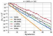
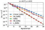
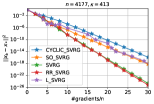
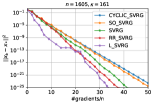
where $A\in\mathbb{R}^{n\times d},y\in\mathbb{R}^{n}$ and $\lambda>0$ is a regularizer. Note that this problem is strongly convex and satisfies the Assumptions 1 for $L=\max_{i}\|A_{i,:}\|^{2}+\lambda$ and $\mu=\frac{\lambda_{\min}(A^{\top}A)}{n}+\lambda$, where $\lambda_{\min}$ is the smallest eigenvalue. To have a tighter bound on the L-smoothness constant we normalize rows of the data matrix $A$. We use datasets from open LIBSVM corpus (Chang & Lin, 2011). In the plots $x$-axis is the number of single data gradient computation divided by $n$, and $y$-axis is the normalized error of the argument $\frac{\|x_{k}-x_{*}\|^{2}}{\|x_{0}-x_{*}\|^{2}}$. In the appendix you can find details and additional experiments.

7.1 Random Reshuffling with Variance Reduction

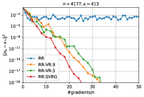
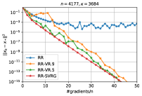
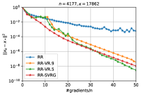
In this subsection, we compare RR from (Mishchenko et al., 2020) and our Algorithm 4. For the Variance Reduced Random Reshuffling algorithm we choose the control update probability $p=0.9$, $p=0.95$ and $p=1$ (RR-SVRG). In our setting, for each algorithm, we choose optimal stepsizes using the grid search. From the plots on Figure 2, we can see that the variance reduction indeed works - RR after some iterations starts to oscillate, while RR-VR version converges to the optimum for all choices of $p$. We also can see that depending on the problem, different values of $p$ could be optimal.

7.2 RR-SVRG vs RR-SAGA

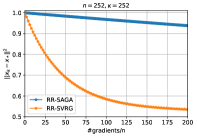
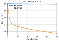
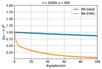
In this experiment, we compare RR-SVRG and RR-SAGA under an academic setting, i.e. we choose the steps that are suggested by theory. For RR-SVRG we take the stepsize $\gamma=\frac{1}{\sqrt{2}Ln}$ when $n\geq\frac{2L}{\mu}\frac{1}{1-\frac{\mu}{\sqrt{2}L}}$ and $\gamma=\frac{1}{2\sqrt{2}Ln}\sqrt{\frac{\mu}{L}}$ otherwise, and for RR-SAGA $\gamma=\frac{\mu}{11L^{2}n}$. We can see that RR-SVRG outperforms RR-SAGA in terms of the number of epochs and the number of gradient computations. Although the cost of iteration of RR-SVRG is twice higher than RR-SAGA, the larger stepsize significantly impacts the total complexity. In addition, RR-SAGA needs $O(nd)$ extra storage to maintain the table of gradients, which makes RR-SAGA algorithm hard to use in the big data regime.

7.3 Variance Reduced Random Reshuffling Algorithms

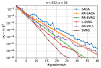
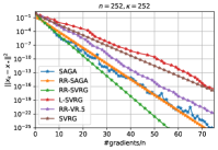
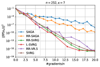
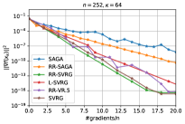
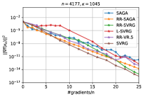
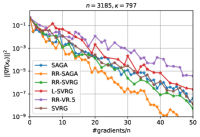
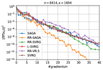
This section compares the variance reduced algorithms with and without random reshuffling: SAGA, RR-SAGA, SVRG, L-SVRG and RR-SVRG. For each algorithm, we choose its optimal stepsizes using the grid search. To make algorithms reasonable to compare in SVRG, we set the length of the inner loop $m=n$, in L-SVRG the control update probability is $1/n$. Also, we consider only the uniform sampling version of SVRG and L-SVRG. We can see the results on Figure 3. We can see that the variance reduced algorithms perform well on this experiment, and there is no obvious leader. However, note that for SAGA and RR-SAGA, we need to have an additional $O(nd)$ space to store the table of the gradients, which is a serious issue in the big data regime.

7.4 Different versions of SVRG

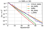
In this section, we compare different types of SVRG algorithm: SVRG, L-SVRG, RR-SVRG, SO-SVRG and CYCLIC-SVRG. For each algorithm we run five experiments with different random seeds with optimal stepsizes found by grid search, then we plot the best of the errors (first and third plots) and the average of the errors (second and fourth plots) on Figure 4. We can see that RR-SVRG in average outperforms other algorithms, while in some random cases L-SVRG can perform better. Also, we can see that SO-SVRG is better than CYCLIC-SVRG that coincides with theoretical findings. If the sampling in each epoch is problematic, one can shuffle data once before the training.

Figure 5: Comparison of SAGA, RR-SAGA, RR-SVRG, L-SVRG, SVRG and RR-VR with $p=0.5$ (RR-VR.5) with optimal stepsizes on bodyfat dataset with different regularization constants (upper left and middle), a1a (upper right), abalone (lower left), a3a (lower middle) and a5a (lower right).

7.5 Experiments with logistic regression

We also run experiments for the regularized logistic regression problem; i.e., for problem (1) with

$$\textstyle f(x)=\frac{1}{n}\sum\limits_{i=1}^{n}\log\left(1+\exp(-y_{i}a_{i}^{\top}x)\right)+\frac{\lambda}{2}\|x\|^{2}.$$

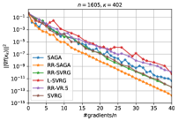
Note that the problem is $L$-smooth and $\mu$-strongly convex for $L=\frac{1}{4n}\lambda_{\max}(A^{\top}A)+\lambda$, and $\mu=\lambda$. In these experiments (also in the ridge regression experiments) when we choose optimal stepsize, we choose the best one among $\{\frac{1}{L},\frac{1}{2L},\frac{1}{3L},\frac{1}{5L},\frac{1}{10L}\}$. For the logistic regression we do not have an explicit formula for the optimum $x_{*}$ as in the ridge regression, thus in this case we compare the norm of the gradients instead. In Figure 5 we can see the performance of the variance reduced algorithms: SAGA, RR-SAGA, SVRG, L-SVRG, RR-VR and RR-SVRG.

8 Conclusion

In this paper, we consider variance-reduced algorithms under random reshuffling. Our results are predominantly theoretical because these algorithms are already widely used in practice and show excellent work. We have provided a first-of-its-kind analysis of SVRG in random reshuffling and cyclic mode. We have proposed a new approach for analysis using inner product reformulation, which leads to better rates. Experimental results confirm our theoretical discoveries. Thus, we receive a deeper theoretical understanding of these algorithms’ work, and we hope that this will inspire researchers to develop further and analyze these methods. The understanding of variance reduction mechanism is essential to construct accelerated versions for stochastic algorithms. We also believe that our theoretical results can be applied to other aspects of machine learning, leading to improvements in state of the art for current or future applications.

Appendix

Appendix A Basic Facts

Proposition 2.

Let $f:\mathbb{R}^{d}\to\mathbb{R}$ be continuously differentiable and let $L\geq 0$. Then the following statements are equivalent:

• $f$ is $L$-smooth,

• $2D_{f}(x,y)\leq L\|x-y\|^{2}\text{ for all }x,y\in\mathbb{R}^{d}$,

• $\langle\nabla f(x)-\nabla f(y),x-y\rangle\leq L\|x-y\|^{2}\text{ for all }x,y\in\mathbb{R}^{d}$.

Proposition 3.

Let $f:\mathbb{R}^{d}\to\mathbb{R}$ be continuously differentiable and let $\mu\geq 0$. Then the following statements are equivalent:

• $f$ is $\mu$-strongly convex,

• $2D_{f}(x,y)\geq\mu\|x-y\|^{2}\text{ for all }x,y\in\mathbb{R}^{d}$,

• $\langle\nabla f(x)-\nabla f(y),x-y\rangle\geq\mu\|x-y\|^{2}\text{ for all }x,y\in\mathbb{R}^{d}$.

Note that the $\mu=0$ case reduces to convexity.

Proposition 4.

Let $f:\mathbb{R}^{d}\to\mathbb{R}$ be continuously differentiable and $L>0$. Then the following statements are equivalent:

• $f$ is convex and $L$-smooth

• $0\leq 2D_{f}(x,y)\leq L\|x-y\|^{2}\text{ for all }x,y\in\mathbb{R}^{d}$,

• $\frac{1}{L}\|\nabla f(x)-\nabla f(y)\|^{2}\leq 2D_{f}(x,y)\text{ for all }x,y\in\mathbb{R}^{d}$,

• $\frac{1}{L}\|\nabla f(x)-\nabla f(y)\|^{2}\leq\langle\nabla f(x)-\nabla f(y),x-y\rangle\text{ for all }x,y\in\mathbb{R}^{d}$.

Proposition 5 (Jensen’s inequality).

Let $f:\mathbb{R}^{d}\to\mathbb{R}$ be a convex function, $x_{1},\ldots,x_{m}\in\mathbb{R}^{d}$ and $\lambda_{1},\ldots,\lambda_{m}$ be nonnegative real numbers adding up to 1. Then

$$f\left(\sum_{i=1}^{m}\lambda_{i}x_{i}\right)\leq\sum_{i=1}^{m}\lambda_{i}f\left(x_{i}\right).$$

Proposition 6.

For all $a,b\in\mathbb{R}^{d}$ and $t>0$ the following inequalities hold

$$\langle a,b\rangle \leq\frac{\|a\|^{2}}{2t}+\frac{t\|b\|^{2}}{2},$$

$$\|a+b\|^{2} \leq 2\|a\|^{2}+2\|b\|^{2},$$

$$\frac{1}{2}\|a\|^{2}-\|b\|^{2} \leq\|a+b\|^{2}.$$

Appendix B From Rate to Iteration Complexity

We use the following standard result often in the paper. We include the statement and proof, for completeness. Assume that some algorithm satisfies the following recursion for some $q\in(0,1)$ and all $t\geq 0$:

$$\mathbb{E}\left[\|x_{t}-x_{*}\|^{2}\right]\leq\left(1-q\right)^{t}\|x_{0}-x_{*}\|^{2}.$$

Then for any $\varepsilon>0$ we have

$$T\geq\frac{1}{q}\ln\left(\frac{1}{\varepsilon}\right)\qquad\Longrightarrow\qquad\mathbb{E}\left[\left\|x^{T}-x^{*}\right\|^{2}\right]\leq\varepsilon\left\|x^{0}-x^{*}\right\|^{2}.$$

Proof.

We know that $e^{q}\geq 1+q,\forall q\in\mathbb{R},\text{ thus }e^{-q}\geq 1-q,\forall q\in(0,1).$ Since the function $\ln$ is increasing over $\mathbb{R}_{+}$, it follows that

$$-q\geq\ln(1-q),\forall q\in(0,1),$$

thus for $t\geq 0$, we get

$$-tq\geq t\ln\left(1-q\right).$$

Now if we have $T$ such that

$$T\geq\frac{1}{q}\ln\left(\frac{1}{\varepsilon}\right),$$

which is equivalent to

$$-T\cdot q\leq\ln(\varepsilon),$$

we obtain

$$T\ln\left(1-q\right)\leq\ln(\varepsilon).$$

Taking exponential on both sides to get

$$0<\left(1-q\right)^{T}\leq\varepsilon.$$

Finally, we have

$$\mathbb{E}\left[\left\|x^{T}-x^{*}\right\|^{2}\right]\leq\left(1-q\right)^{T}\left\|x^{0}-x^{*}\right\|^{2}\leq\varepsilon\left\|x^{0}-x^{*}\right\|^{2}.$$

This leads to

$$T\geq\frac{1}{q}\ln\left(\frac{1}{\varepsilon}\right)\Longrightarrow\mathbb{E}\left\|x^{T}-x^{*}\right\|^{2}\leq\varepsilon\left\|x^{0}-x^{*}\right\|^{2}.$$

∎

Appendix C Proof of Proposition 1

Assume that each $f_{i}$ is $\mu$-strongly convex (convex) and $L$-smooth. Then $\tilde{f}$ defined as

$$\tilde{f}_{i}(x)=f_{i}(x)+\left\langle a_{i},x\right\rangle$$ (10)

is $\mu$-strongly convex (convex) and $L$-smooth.

Proof.

Let us compute Bregman divergence with respect to the new function $\tilde{f}_{i}(x):$

$$D_{\tilde{f}_{i}}(x,y)=\tilde{f}_{i}(x)-\tilde{f}_{i}(y)-\langle\nabla\tilde{f}_{i}(y),x-y\rangle.$$

Note that $\nabla\tilde{f}_{i}(y)=\nabla f_{i}(y)+a_{i}$. Now we have

$$D_{\tilde{f}_{i}}(x,y) =\tilde{f}_{i}(x)-\tilde{f}_{i}(y)-\langle\nabla\tilde{f}_{i}(y),x-y\rangle$$

$$=f_{i}(x)+\left\langle a_{i},x\right\rangle-\left(f_{i}(y)+\left\langle a_{i},y\right\rangle\right)-\langle\nabla f_{i}(y)+a_{i},x-y\rangle$$

$$=f_{i}(x)+\left\langle a_{i},x\right\rangle-f_{i}(y)-\left\langle a_{i},y\right\rangle-\langle\nabla f_{i}(y),x-y\rangle-\langle a_{i},x-y\rangle$$

$$=f_{i}(x)+\left\langle a_{i},x\right\rangle-f_{i}(y)-\left\langle a_{i},y\right\rangle-\langle\nabla f_{i}(y),x-y\rangle-\langle a_{i},x\rangle+\langle a_{i},y\rangle$$

$$=f_{i}(x)-f_{i}(y)-\langle\nabla f_{i}(y),x-y\rangle$$

$$=D_{f_{i}}(x,y).$$

Since the Bregman divergence is not changed, the new function $\tilde{f}_{i}(x)$ has the same properties ($\mu$-strong convexity or convexity and $L$-smoothness) as the initial function $f_{i}(x)$. ∎

Appendix D Proof of Lemma 1

Assume that each $f_{i}$ is $L$-smooth and convex. If we apply the linear perturbation reformulation (7) using vectors of the form $a_{i}=-\nabla f_{\pi_{i}}(y_{t})+\nabla f(y_{t})$, then the variance of reformulated problem satisfies the following inequality:

$$\tilde{\sigma}_{*}^{2}=\frac{1}{n}\sum\limits_{i=1}^{n}\left\|\nabla\tilde{f}_{i}\left(x_{*}\right)\right\|^{2}\leq 4L^{2}\|y_{t}-x_{*}\|^{2}.$$ (11)

Proof.

Let us start from the definition:

$$\tilde{\sigma}_{*}^{2} =\frac{1}{n}\sum_{i=1}^{n}\|\nabla\tilde{f}_{i}(x_{*})\|^{2}$$

$$=\frac{1}{n}\sum_{i=1}^{n}\|\nabla f_{i}(x_{*})-\nabla f_{i}(y_{t})+\nabla f(y_{t})\|^{2}$$

$$=\frac{1}{n}\sum_{i=1}^{n}\|\nabla f_{i}(x_{*})-\nabla f_{i}(y_{t})+\nabla f(y_{t})-\nabla f(x_{*})\|^{2}.$$

Using Young’s inequality, we get

$$\tilde{\sigma}_{*}^{2} \leq\frac{1}{n}\sum_{i=1}^{n}\left(2\|\nabla f_{i}(y_{t})-\nabla f_{i}(x_{*})\|^{2}+2\|\nabla f(y_{t})-\nabla f(x_{*})\|^{2}\right)$$

$$\leq\frac{1}{n}\sum_{i=1}^{n}4L_{i}D_{f_{i}}(y_{t},x_{*})+\frac{1}{n}\sum_{i=1}^{n}4LD_{f}(y_{t},x_{*})$$

$$\leq 4LD_{f}(y_{t},x_{*})+4LD_{f}(y_{t},x_{*})$$

$$=8LD_{f}(y_{t},x_{*})$$

$$\leq 4L^{2}\|y_{t}-x_{*}\|^{2}.$$

∎

Appendix E Analysis of Algorithms 1 and 2

E.1 Proof of Theorems 1 and 2

Suppose that each $f_{i}$ is convex, $f$ is $\mu$-strongly convex, and Assumption 1 holds. Then provided the stepsize satisfies $\gamma\leq\frac{1}{2\sqrt{2}Ln}\sqrt{\frac{\mu}{L}},$ the iterates generated by RR-SVRG (Algorithm 1) or by SO-SVRG (Algorithm 2) satisfy

$$\mathbb{E}\left[\|x_{T}-x_{*}\|^{2}\right]\leq\left(1-\frac{\gamma n\mu}{2}\right)^{T}\|x_{0}-x_{*}\|^{2}.$$

Suppose that each $f_{i}$ is convex, $f$ is $\mu$-strongly convex and Assumption 1 holds. Additionally assume we are in the “big data” regime characterized by $n\geq\frac{2L}{\mu}\cdot\frac{1}{1-\frac{\mu}{\sqrt{2}L}}$. Then provided the stepsize satisfies $\gamma\leq\frac{1}{\sqrt{2}Ln},$ the iterates generated by RR-SVRG (Algorithm 1) or by SO-SVRG (Algorithm 2) satisfy

$$\mathbb{E}\left[\|x_{T}-x_{*}\|^{2}\right]\leq\left(1-\frac{\gamma n\mu}{2}\right)^{T}\|x_{0}-x_{*}\|^{2}.$$

Proof.

We start from Lemma 3 in paper of Mishchenko et al. (2020).

Lemma 3. Assume that functions $f_{1},\ldots,f_{n}$ are convex and that Assumption 1 is satisfied. If Random Reshuffling or Shuffle-Once is run with a stepsize satisfying $\gamma\leq\frac{1}{\sqrt{2}Ln}$, then

$$\mathbb{E}\left[\left\|x_{t+1}-x_{*}\right\|^{2}\right]\leq\mathbb{E}\left[\left\|x_{t}-x_{*}\right\|^{2}\right]-2\gamma n\mathbb{E}\left[f\left(x_{t+1}\right)-f(x_{*})\right]+\frac{\gamma^{3}Ln^{2}\sigma_{*}^{2}}{2}.$$

Now we can apply to the reformulated problem (7). Using strong convexity we obtain

$$\mathbb{E}\left[\left\|x_{t+1}-x_{*}\right\|^{2}\mid x_{t}\right] \leq\left\|x_{t}-x_{*}\right\|^{2}-2\gamma n\mathbb{E}\left[f\left(x_{t+1}\right)-f(x_{*})\mid x_{t}\right]+\frac{\gamma^{3}Ln^{2}\tilde{\sigma}_{*}^{2}}{2}$$

$$\leq\left\|x_{t}-x_{*}\right\|^{2}-\gamma n\mu\mathbb{E}\left[\left\|x_{t+1}-x_{*}\right\|^{2}\mid x_{t}\right]+\frac{\gamma^{3}Ln^{2}\tilde{\sigma}_{*}^{2}}{2}.$$

For Algorithms 1 and 2 we update $y_{t}=x_{t}$ after each epoch, and this leads to

$$\mathbb{E}\left[\left\|x_{t+1}-x_{*}\right\|^{2}\mid x_{t}\right] \leq\frac{1}{1+\gamma\mu n}\left(\left\|x_{t}-x_{*}\right\|^{2}+\frac{\gamma^{3}Ln^{2}\tilde{\sigma}_{*}^{2}}{2}\right)$$

$$\leq\frac{1}{1+\gamma\mu n}\left(\left\|x_{t}-x_{*}\right\|^{2}+\frac{\gamma^{3}Ln^{2}\cdot 4L^{2}\|y_{t}-x_{*}\|^{2}}{2}\right)$$

$$=\frac{1}{1+\gamma\mu n}\left(\left\|x_{t}-x_{*}\right\|^{2}+2\gamma^{3}n^{2}L^{3}\|x_{t}-x_{*}\|^{2}\right)$$

$$=\frac{1}{1+\gamma\mu n}\left(1+2\gamma^{3}n^{2}L^{3}\right)\|x_{t}-x_{*}\|^{2}.$$

We can use the tower property to obtain

$$\mathbb{E}\left[\left\|x_{t+1}-x_{*}\right\|^{2}\right]\leq\frac{1+2\gamma^{3}L^{3}n^{2}}{1+\gamma\mu n}\mathbb{E}\left[\left\|x_{t}-x_{*}\right\|^{2}\right].$$

If this inequality $\frac{1+2\gamma^{3}L^{3}n^{2}}{1+\gamma\mu n}\leq 1-\frac{\gamma n\mu}{2}$ is correct, we can unroll the recursion and obtain

$$\mathbb{E}\left[\|x_{T}-x_{*}\|^{2}\right]\leq\left(1-\frac{\gamma n\mu}{2}\right)^{T}\|x_{0}-x_{*}\|^{2}.$$

Now we need to solve the following inequality:

$$\frac{1+2\gamma^{3}L^{3}n^{2}}{1+\gamma\mu n}\leq 1-\frac{\gamma n\mu}{2}.$$

Let us simplify it:

$$1+2\gamma^{3}L^{3}n^{2} \leq 1+\frac{\gamma n\mu}{2}-\frac{\gamma^{2}n^{2}\mu^{2}}{2}$$

$$2\gamma^{2}L^{3}n^{2} \leq\frac{n\mu}{2}-\frac{\gamma n^{2}\mu^{2}}{2}$$

$$2\gamma^{2}L^{3}n \leq\frac{\mu}{2}-\frac{\gamma n\mu^{2}}{2}$$

$$2\gamma^{2}L^{3}n+\frac{\gamma n\mu^{2}}{2} \leq\frac{\mu}{2}.$$

Now as $\gamma\leq\frac{1}{2\sqrt{2}Ln}\sqrt{\frac{\mu}{L}}$, we have

$$2\cdot\frac{1}{8L^{2}n^{2}}\cdot\frac{\mu}{L}L^{3}n+\frac{1}{2\sqrt{2}Ln}\sqrt{\frac{\mu}{L}}\cdot\frac{n\mu^{2}}{2} \leq\frac{\mu}{2}$$

$$\frac{1}{4n}\mu+\frac{1}{4\sqrt{2}}\frac{\mu}{L}\sqrt{\frac{\mu}{L}}\mu \leq\frac{\mu}{2}$$

$$\frac{1}{4n}+\frac{1}{4\sqrt{2}}\frac{\mu}{L}\sqrt{\frac{\mu}{L}} \leq\frac{1}{2}.$$

It is true since $n\geq 1$ and $\mu\leq L$. This ends proof of Theorem 1.

Now let us use the biggest step-size allowed by the Lemma 3 in Section E.1. Let us utilize $\gamma\leq\frac{1}{\sqrt{2}Ln}:$

$$2\cdot\frac{1}{2L^{2}n^{2}}L^{3}n+\frac{1}{\sqrt{2}Ln}\cdot\frac{n\mu^{2}}{2} \leq\frac{\mu}{2}$$

$$\frac{L}{n}+\frac{\mu}{2}\cdot\frac{\mu}{\sqrt{2}L} \leq\frac{\mu}{2}.$$

This leads to

$$\frac{L}{n} \leq\frac{\mu}{2}-\frac{\mu}{2}\cdot\frac{\mu}{\sqrt{2}L}=\frac{\mu}{2}\left(1-\frac{\mu}{\sqrt{2}L}\right)$$

and

$$\frac{1}{n}\leq\frac{\mu}{2L}\left(1-\frac{\mu}{\sqrt{2}L}\right)\quad\Rightarrow\quad n\geq\frac{2L}{\mu}\cdot\frac{1}{1-\frac{\mu}{\sqrt{2}L}}.$$

That is the end of Theorem 2. ∎

The proofs of Corollary 1 and 2 is a simple application of the lemma from Section B.

E.2 Proof of Theorem 3

Suppose that the functions $f_{1},\ldots,f_{n}$ are $\mu$-strongly convex and Assumption 1 holds. Fix constant $0<\delta<1$. If the stepsize satisfies $\gamma\leq\frac{\delta}{L}\sqrt{\frac{\mu}{2nL}}$ and if number of functions is sufficiently big,

$$n>\log\left(\frac{1}{1-\delta^{2}}\right)\cdot\left(\log\left(\frac{1}{1-\gamma\mu}\right)\right)^{-1},$$

then the iterates generated by RR-SVRG (Algorithm 1) or by SO-SVRG (Algorithm 2) satisfy

$$\mathbb{E}\left[\|x_{T}-x_{*}\|^{2}\right]\leq\left(\left(1-\gamma\mu\right)^{n}+\delta^{2}\right)^{T}\|x_{0}-x_{*}\|^{2}.$$

Proof.

We start from Theorem 1 in paper of Mishchenko et al. (2020):

$$\mathbb{E}\left[\left\|x_{t+1}-x_{*}\right\|^{2}\mid x_{t}\right]\leq(1-\gamma\mu)^{n}\left\|x_{t}-x_{*}\right\|^{2}+2\gamma^{2}\sigma_{\text{Shuffle }}^{2}\left(\sum_{i=0}^{n-1}(1-\gamma\mu)^{i}\right).$$

Using Preposition 1 in paper of Mishchenko et al. (2020):

$$\frac{\gamma\mu n}{8}\sigma_{*}^{2}\leq\sigma_{\text{Shuffle }}^{2}\leq\frac{\gamma Ln}{4}\sigma_{*}^{2},$$

we have

$$\mathbb{E}\left[\left\|x_{t+1}-x_{*}\right\|^{2}\mid x_{t}\right]\leq(1-\gamma\mu)^{n}\left\|x_{t}-x_{*}\right\|^{2}+\frac{\gamma^{3}Ln}{2}\sigma_{*}^{2}\left(\sum_{i=0}^{n-1}(1-\gamma\mu)^{i}\right).$$

Using property of geometric progression we can have an upper bound for the sum $\sum_{i=0}^{n-1}(1-\gamma\mu)^{i}\leq\frac{1}{\gamma\mu}$:

$$\mathbb{E}\left[\left\|x_{t+1}-x_{*}\right\|^{2}\mid x_{t}\right]\leq(1-\gamma\mu)^{n}\left\|x_{t}-x_{*}\right\|^{2}+\frac{\gamma^{2}Ln}{2\mu}\sigma_{*}^{2}.$$

Now we can apply Lemma 1 and using $y_{t}=x_{t}$ we have the following inequality:

$$\mathbb{E}\left[\left\|x_{t+1}-x_{*}\right\|^{2}\mid x_{t}\right] \leq(1-\gamma\mu)^{n}\left\|x_{t}-x_{*}\right\|^{2}+\frac{2\gamma^{2}L^{3}n}{\mu}\|x_{t}-x_{*}\|^{2}$$

$$\mathbb{E}\left[\left\|x_{t+1}-x_{*}\right\|^{2}\mid x_{t}\right] \leq\left((1-\gamma\mu)^{n}+\frac{2\gamma^{2}L^{3}n}{\mu}\right)\|x_{t}-x_{*}\|^{2}.$$

Now we utilize tower property:

$$\mathbb{E}\left[\left\|x_{t+1}-x_{*}\right\|^{2}\right] \leq\left((1-\gamma\mu)^{n}+\frac{2\gamma^{2}L^{3}n}{\mu}\right)\mathbb{E}\left[\|x_{t}-x_{*}\|^{2}\right].$$

Unrolling this recursion we get:

$$\mathbb{E}\left[\left\|x_{T}-x_{*}\right\|^{2}\right] \leq\left((1-\gamma\mu)^{n}+\frac{2\gamma^{2}L^{3}n}{\mu}\right)^{T}\mathbb{E}\left[\|x_{0}-x_{*}\|^{2}\right].$$

Let us use $\gamma\leq\frac{\delta}{L}\sqrt{\frac{\mu}{2nL}}$:

$$\mathbb{E}\left[\left\|x_{T}-x_{*}\right\|^{2}\right] \leq\left((1-\gamma\mu)^{n}+\frac{\delta^{2}}{L^{2}}\frac{\mu}{2nL}\frac{2L^{3}n}{\mu}\right)^{T}\mathbb{E}\left[\|x_{0}-x_{*}\|^{2}\right]$$

$$\mathbb{E}\left[\left\|x_{T}-x_{*}\right\|^{2}\right] \leq\left((1-\gamma\mu)^{n}+\delta^{2}\right)^{T}\mathbb{E}\left[\|x_{0}-x_{*}\|^{2}\right].$$

To get convergence we need:

$$(1-\gamma\mu)^{n}+\delta^{2}<1.$$

This leads to the following inequality:

$$n>\log\left(\frac{1}{1-\delta^{2}}\right)\cdot\left(\log\left(\frac{1}{1-\gamma\mu}\right)\right)^{-1}$$

This ends the proof.

E.3 Proof of Corollary 3

Suppose that assumptions in Theorem 3 hold. Additionally assume that $n$ is large enough to satisfy the inequality $\delta^{2}\leq(1-\gamma\mu)^{\frac{n}{2}}\left(1-(1-\gamma\mu)^{\frac{n}{2}}\right)$. Then the iteration complexity of Algorithms 1 and 2 is

$$T=\mathcal{O}\left(\kappa\sqrt{\frac{\kappa}{n}}\log\left(\frac{1}{\varepsilon}\right)\right).$$

Proof.

Using the additional assumption $\delta^{2}\leq(1-\gamma\mu)^{\frac{n}{2}}\left(1-(1-\gamma\mu)^{\frac{n}{2}}\right),$ we get

$$\delta^{2}+(1-\gamma\mu)^{n}\leq(1-\gamma\mu)^{\frac{n}{2}}.$$

Now we can apply Theorem 3 and get

$$\mathbb{E}\left[\|x_{T}-x_{*}\|^{2}\right]\leq\left(1-\gamma\mu\right)^{\frac{nT}{2}}\|x_{0}-x_{*}\|^{2}.$$

Finally, we apply the lemma from Section B with $\gamma\leq\frac{\delta}{L}\sqrt{\frac{\mu}{2nL}}$ and get

$$T=\mathcal{O}\left(\kappa\sqrt{\frac{\kappa}{n}}\log\left(\frac{1}{\varepsilon}\right)\right).$$

∎

E.4 Proof of Theorem 4

Suppose the functions $f_{1},f_{2},\ldots,f_{n}$ are convex and Assumption 1 holds. Then for RR-SVRG (Algorithm 1) or SO-SVRG (Algorithm 2) with stepsize $\gamma\leq\frac{1}{\sqrt{2}Ln},$ the average iterate $\hat{x}_{T}\coloneqq\frac{1}{T}\sum_{t=1}^{T}x_{t}$ satisfies

$$\mathbb{E}\left[f\left(\hat{x}_{T}\right)-f\left(x_{*}\right)\right]\leq\frac{3\left\|x_{0}-x_{*}\right\|^{2}}{2\gamma nT}.$$

Proof.

We start with Lemma 3 from Mishchenko et al. (2020):

$$\mathbb{E}\left[\left\|x_{t+1}-x_{*}\right\|^{2}\mid x_{t}\right]\leq\left\|x_{t}-x_{*}\right\|^{2}-2\gamma n\mathbb{E}\left[f\left(x_{t+1}\right)-f\left(x_{*}\right)\mid x_{t}\right]+\frac{\gamma^{3}Ln^{2}\sigma_{*}^{2}}{2}$$

$$2\gamma n\mathbb{E}\left[f\left(x_{t+1}\right)-f\left(x_{*}\right)\mid x_{t}\right]\leq\left\|x_{t}-x_{*}\right\|^{2}-\mathbb{E}\left[\left\|x_{t+1}-x_{*}\right\|^{2}\mid x_{t}\right]+\frac{\gamma^{3}Ln^{2}\sigma_{*}^{2}}{2}.$$

Using Lemma 1 and considering $y_{t}=x_{t}$ we have

$$\tilde{\sigma}_{*}^{2}\leq 8LD_{\tilde{f}}(x_{t},x_{*}).$$

Applying Proposition 1 we get

$$\tilde{\sigma}_{*}^{2}\leq 8LD_{f}(x_{t},x_{*})=8L(f(x_{t})-f(x_{*})).$$

Next, we utilize the inner product reformulation and get

$$2\gamma n\mathbb{E}\left[f\left(x_{t+1}\right)-f\left(x_{*}\right)\mid x_{t}\right]\leq\left\|x_{t}-x_{*}\right\|^{2}-\mathbb{E}\left[\left\|x_{t+1}-x_{*}\right\|^{2}\mid x_{t}\right]+\frac{\gamma^{3}Ln^{2}}{2}\cdot 8L(f(x_{t})-f(x_{*})).$$

Using tower property we have

$$2\gamma n\mathbb{E}\left[f\left(x_{t+1}\right)-f\left(x_{*}\right)\right]\leq\mathbb{E}\left[\left\|x_{t}-x_{*}\right\|^{2}\right]-\mathbb{E}\left[\left\|x_{t+1}-x_{*}\right\|^{2}\right]+4\gamma^{3}L^{2}n^{2}\mathbb{E}\left[f(x_{t})-f(x_{*})\right].$$

Now we subtract from both sides:

$$2\gamma n\mathbb{E}\left[f\left(x_{t+1}\right)-f\left(x_{*}\right)\right]-4\gamma^{3}L^{2}n^{2}\mathbb{E}\left[f\left(x_{t+1}\right)-f\left(x_{*}\right)\right] \leq\mathbb{E}\left[\left\|x_{t}-x_{*}\right\|^{2}\right]-\mathbb{E}\left[\left\|x_{t+1}-x_{*}\right\|^{2}\right]$$

$$\qquad+4\gamma^{3}L^{2}n^{2}\mathbb{E}\left[f(x_{t})-f(x_{*})\right]$$

$$\qquad-4\gamma^{3}L^{2}n^{2}\mathbb{E}\left[f\left(x_{t+1}\right)-f\left(x_{*}\right)\right]$$

$$\left(2\gamma n-4\gamma^{3}L^{2}n^{2}\right)\mathbb{E}\left[f\left(x_{t+1}\right)-f\left(x_{*}\right)\right] \leq\mathbb{E}\left[\left\|x_{t}-x_{*}\right\|^{2}\right]-\mathbb{E}\left[\left\|x_{t+1}-x_{*}\right\|^{2}\right]$$

$$\qquad+4\gamma^{3}L^{2}n^{2}\left(\mathbb{E}\left[f(x_{t})-f(x_{*})\right]-\mathbb{E}\left[f\left(x_{t+1}\right)-f\left(x_{*}\right)\right]\right)$$

$$2\gamma n\left(1-2\gamma^{2}L^{2}n\right)\mathbb{E}\left[f\left(x_{t+1}\right)-f\left(x_{*}\right)\right] \leq\mathbb{E}\left[\left\|x_{t}-x_{*}\right\|^{2}\right]-\mathbb{E}\left[\left\|x_{t+1}-x_{*}\right\|^{2}\right]$$

$$\qquad+4\gamma^{3}L^{2}n^{2}\left(\mathbb{E}\left[f(x_{t})-f(x_{*})\right]-\mathbb{E}\left[f\left(x_{t+1}\right)-f\left(x_{*}\right)\right]\right).$$

Summing these inequalities for $t=0,1,\ldots,T-1$ gives

$$2\gamma n\left(1-2\gamma^{2}L^{2}n\right)\sum_{t=0}^{T-1}\mathbb{E}\left[f\left(x_{t+1}\right)-f\left(x_{*}\right)\right] \leq\sum_{t=0}^{T-1}\left(\mathbb{E}\left[\left\|x_{t}-x_{*}\right\|^{2}\right]-\mathbb{E}\left[\left\|x_{t+1}-x_{*}\right\|^{2}\right]\right)$$

$$\qquad+4\gamma^{3}L^{2}n^{2}\sum_{t=0}^{T-1}\left(\mathbb{E}\left[f(x_{t})-f(x_{*})\right]-\mathbb{E}\left[f\left(x_{t+1}\right)-f\left(x_{*}\right)\right]\right)$$

$$=\mathbb{E}\left[\left\|x_{0}-x_{*}\right\|^{2}\right]-\mathbb{E}\left[\left\|x_{T}-x_{*}\right\|^{2}\right]$$

$$\qquad+4\gamma^{3}L^{2}n^{2}\mathbb{E}\left[f\left(x_{0}\right)-f\left(x_{*}\right)\right]-4\gamma^{3}L^{2}n^{2}\mathbb{E}\left[f\left(x_{T}\right)-f\left(x_{*}\right)\right]$$

$$\leq\mathbb{E}\left[\left\|x_{0}-x_{*}\right\|^{2}\right]+4\gamma^{3}L^{2}n^{2}\mathbb{E}\left[f\left(x_{0}\right)-f\left(x_{*}\right)\right]$$

$$\leq\mathbb{E}\left[\left\|x_{0}-x_{*}\right\|^{2}\right]+2\gamma^{3}L^{3}n^{2}\mathbb{E}\left[\left\|x_{0}-x_{*}\right\|^{2}\right]$$

$$=(1+2\gamma^{3}L^{3}n^{2})\mathbb{E}\left[\left\|x_{0}-x_{*}\right\|^{2}\right],$$

and dividing both sides by $2\gamma n\left(1-2\gamma^{2}L^{2}n\right)T$, we get

$$\frac{1}{T}\sum_{t=0}^{T-1}\mathbb{E}\left[f\left(x_{t+1}\right)-f\left(x_{*}\right)\right] \leq\frac{1+2\gamma^{3}L^{3}n^{2}}{1-2\gamma^{2}L^{2}n}\frac{\left\|x_{0}-x_{*}\right\|^{2}}{2\gamma nT}.$$

Using the convexity of $f$, the average iterate $\hat{x}_{T}\stackrel{{\scriptstyle\text{ def }}}{{=}}\frac{1}{T}\sum_{t=1}^{T}x_{t}$ satisfies

$$\mathbb{E}\left[f\left(\hat{x}_{T}\right)-f\left(x_{*}\right)\right]\leq\frac{1}{T}\sum_{t=1}^{T}\mathbb{E}\left[f\left(x_{t}\right)-f\left(x_{*}\right)\right]\leq\frac{1+2\gamma^{3}L^{3}n^{2}}{1-2\gamma^{2}L^{2}n}\frac{\left\|x_{0}-x_{*}\right\|^{2}}{2\gamma nT}.$$

Let us show that

$$\frac{1+2\gamma^{3}L^{3}n^{2}}{1-2\gamma^{2}L^{2}n}\leq 3.$$

Applying $\gamma\leq\frac{1}{\sqrt{2}Ln}$ we have

$$\frac{1+2\frac{1}{2\sqrt{2}L^{3}n^{3}}L^{3}n^{2}}{1-2\frac{1}{2L^{2}n^{2}}L^{2}n}=\frac{1+\frac{1}{\sqrt{2}n}}{1-\frac{1}{n}}\leq 3.$$

This leads to $4n>6+\sqrt{2}$ and since $n\in\mathbb{N}:n>1$, this inequality holds. Finally, we have

$$\mathbb{E}\left[f\left(\hat{x}_{T}\right)-f\left(x_{*}\right)\right]\leq\frac{3\left\|x_{0}-x_{*}\right\|^{2}}{2\gamma nT}.$$

∎

This ends the proof. The Corollary 4 is a simple application of Theorem 4

Appendix F Analysis of Algorithm 3

F.1 Proof of Theorem 5

Suppose that each $f_{i}$ is convex function, $f$ is $\mu$-strongly convex function, and Assumption 1 holds. Then provided the stepsize satisfies $\gamma\leq\frac{1}{4Ln}\sqrt{\frac{\mu}{L}},$ the iterates generated by Cyclic SVRG (Algorithm 3) satisfy

$$\mathbb{E}\left[\|x_{T}-x_{*}\|^{2}\right]\leq\left(1-\frac{\gamma n\mu}{2}\right)^{T}\|x_{0}-x_{*}\|^{2}.$$

We start from Lemma 8 in Mishchenko et al. (2020)

$$\left\|x_{t+1}-x_{*}\right\|^{2}\leq\left\|x_{t}-x_{*}\right\|^{2}-2\gamma n\left(f\left(x_{t+1}\right)-f\left(x_{*}\right)\right)+\gamma^{3}Ln^{3}\sigma_{*}^{2}.$$ (12)

Now we can apply to the reformulated problem (7). Using strong convexity we obtain

$$\mathbb{E}\left[\left\|x_{t+1}-x_{*}\right\|^{2}\mid x_{t}\right] \leq\left\|x_{t}-x_{*}\right\|^{2}-2\gamma n\mathbb{E}\left[f\left(x_{t+1}\right)-f(x_{*})\mid x_{t}\right]+\gamma^{3}Ln^{2}\tilde{\sigma}_{*}^{2}$$

$$\leq\left\|x_{t}-x_{*}\right\|^{2}-\gamma n\mu\mathbb{E}\left[\left\|x_{t+1}-x_{*}\right\|^{2}\mid x_{t}\right]+\gamma^{3}Ln^{3}\tilde{\sigma}_{*}^{2}.$$

For algorithms 1 and 2 we update $y_{t}=x_{t}$ after each epoch, this leads to

$$\mathbb{E}\left[\left\|x_{t+1}-x_{*}\right\|^{2}\mid x_{t}\right] \leq\frac{1}{1+\gamma\mu n}\left(\left\|x_{t}-x_{*}\right\|^{2}+\gamma^{3}Ln^{3}\tilde{\sigma}_{*}^{2}\right)$$

$$\leq\frac{1}{1+\gamma\mu n}\left(\left\|x_{t}-x_{*}\right\|^{2}+\gamma^{3}Ln^{3}\cdot 4L^{2}\|y_{t}-x_{*}\|^{2}\right)$$

$$=\frac{1}{1+\gamma\mu n}\left(\left\|x_{t}-x_{*}\right\|^{2}+4\gamma^{3}n^{3}L^{3}\|x_{t}-x_{*}\|^{2}\right)$$

$$=\frac{1}{1+\gamma\mu n}\left(1+4\gamma^{3}n^{3}L^{3}\right)\|x_{t}-x_{*}\|^{2}.$$

We can use the tower property to obtain

$$\mathbb{E}\left[\left\|x_{t+1}-x_{*}\right\|^{2}\right]\leq\frac{1+4\gamma^{3}L^{3}n^{3}}{1+\gamma\mu n}\mathbb{E}\left[\left\|x_{t}-x_{*}\right\|^{2}\right].$$

If this inequality $\frac{1+4\gamma^{3}L^{3}n^{3}}{1+\gamma\mu n}\leq 1-\frac{\gamma n\mu}{2}$ is correct, we can unroll the recursion and obtain

$$\mathbb{E}\left[\|x_{T}-x_{*}\|^{2}\right]\leq\left(1-\frac{\gamma n\mu}{2}\right)^{T}\|x_{0}-x_{*}\|^{2}.$$

Now we need to solve the following inequality:

$$\frac{1+4\gamma^{3}L^{3}n^{3}}{1+\gamma\mu n}\leq 1-\frac{\gamma n\mu}{2}.$$

Let us simplify it:

$$1+4\gamma^{3}L^{3}n^{3} \leq 1+\frac{\gamma n\mu}{2}-\frac{\gamma^{2}n^{2}\mu^{2}}{2}$$

$$4\gamma^{2}L^{3}n^{3} \leq\frac{n\mu}{2}-\frac{\gamma n^{2}\mu^{2}}{2}$$

$$4\gamma^{2}L^{3}n^{2} \leq\frac{\mu}{2}-\frac{\gamma n\mu^{2}}{2}$$

$$4\gamma^{2}L^{3}n^{2}+\frac{\gamma n\mu^{2}}{2} \leq\frac{\mu}{2}.$$

Now as $\gamma\leq\frac{1}{4Ln}\sqrt{\frac{\mu}{L}}$, we have

$$2\cdot\frac{1}{16L^{2}n^{2}}\cdot\frac{\mu}{L}L^{3}n^{2}+\frac{1}{4Ln}\sqrt{\frac{\mu}{L}}\cdot\frac{n\mu^{2}}{2} \leq\frac{\mu}{2}$$

$$\frac{1}{4}\mu+\frac{1}{8}\frac{\mu}{L}\sqrt{\frac{\mu}{L}}\mu \leq\frac{\mu}{2}$$

$$\frac{1}{4}+\frac{1}{8}\frac{\mu}{L}\sqrt{\frac{\mu}{L}} \leq\frac{1}{2}.$$

It is true since $n\geq 1$ and $\mu\leq L$. This ends proof of Theorem 5. ∎ The proofs of Corollary 5 is a simple application of the lemma from Section B.

F.2 Proof of Theorem 6

Suppose the functions $f_{1},f_{2},\ldots,f_{n}$ are convex and Assumption 1 hold.s Then for Algorithm 3 with a stepsize $\gamma\leq\frac{1}{2\sqrt{2}Ln}$, the average iterate $\hat{x}_{T}\coloneqq\frac{1}{T}\sum_{j=1}^{T}x_{j}$ satisfies

$$\mathbb{E}\left[f\left(\hat{x}_{T}\right)-f\left(x_{*}\right)\right]\leq\frac{2\left\|x_{0}-x_{*}\right\|^{2}}{\gamma nT}.$$

We start with Lemma 8 from Mishchenko et al. (2020):

$$\mathbb{E}\left[\left\|x_{t+1}-x_{*}\right\|^{2}\mid x_{t}\right]\leq\left\|x_{t}-x_{*}\right\|^{2}-2\gamma n\mathbb{E}\left[f\left(x_{t+1}\right)-f\left(x_{*}\right)\mid x_{t}\right]+\gamma^{3}Ln^{3}\sigma_{*}^{2}$$

$$2\gamma n\mathbb{E}\left[f\left(x_{t+1}\right)-f\left(x_{*}\right)\mid x_{t}\right]\leq\left\|x_{t}-x_{*}\right\|^{2}-\mathbb{E}\left[\left\|x_{t+1}-x_{*}\right\|^{2}\mid x_{t}\right]+\gamma^{3}Ln^{3}\sigma_{*}^{2}.$$

Using Lemma 1 and considering $y_{t}=x_{t}$, we have

$$\tilde{\sigma}_{*}^{2}\leq 8LD_{\tilde{f}}(x_{t},x_{*}).$$

Applying Proposition 1 we get

$$\tilde{\sigma}_{*}^{2}\leq 8LD_{f}(x_{t},x_{*})=8L(f(x_{t})-f(x_{*})).$$

Next, we utilize the inner product reformulation and get

$$2\gamma n\mathbb{E}\left[f\left(x_{t+1}\right)-f\left(x_{*}\right)\mid x_{t}\right]\leq\left\|x_{t}-x_{*}\right\|^{2}-\mathbb{E}\left[\left\|x_{t+1}-x_{*}\right\|^{2}\mid x_{t}\right]+\gamma^{3}Ln^{3}\cdot 8L(f(x_{t})-f(x_{*})).$$

Using tower property we have

$$2\gamma n\mathbb{E}\left[f\left(x_{t+1}\right)-f\left(x_{*}\right)\right]\leq\mathbb{E}\left[\left\|x_{t}-x_{*}\right\|^{2}\right]-\mathbb{E}\left[\left\|x_{t+1}-x_{*}\right\|^{2}\right]+8\gamma^{3}L^{2}n^{3}\mathbb{E}\left[(f(x_{t})-f(x_{*}))\right].$$

Now we subtract from both sides:

$$2\gamma n\mathbb{E}\left[f\left(x_{t+1}\right)-f\left(x_{*}\right)\right]-8\gamma^{3}L^{2}n^{3}\mathbb{E}\left[f\left(x_{t+1}\right)-f\left(x_{*}\right)\right] \leq\mathbb{E}\left[\left\|x_{t}-x_{*}\right\|^{2}\right]-\mathbb{E}\left[\left\|x_{t+1}-x_{*}\right\|^{2}\right]$$

$$\qquad+8\gamma^{3}L^{2}n^{3}\mathbb{E}\left[(f(x_{t})-f(x_{*}))\right]$$

$$\qquad-8\gamma^{3}L^{2}n^{3}\mathbb{E}\left[f\left(x_{t+1}\right)-f\left(x_{*}\right)\right]$$

$$\left(2\gamma n-8\gamma^{3}L^{2}n^{3}\right)\mathbb{E}\left[f\left(x_{t+1}\right)-f\left(x_{*}\right)\right] \leq\mathbb{E}\left[\left\|x_{t}-x_{*}\right\|^{2}\right]-\mathbb{E}\left[\left\|x_{t+1}-x_{*}\right\|^{2}\right]$$

$$\qquad+8\gamma^{3}L^{2}n^{3}\left(\mathbb{E}\left[f(x_{t})-f(x_{*})\right]-\mathbb{E}\left[f\left(x_{t+1}\right)-f\left(x_{*}\right)\right]\right)$$

$$2\gamma n\left(1-4\gamma^{2}L^{2}n^{2}\right)\mathbb{E}\left[f\left(x_{t+1}\right)-f\left(x_{*}\right)\right] \leq\mathbb{E}\left[\left\|x_{t}-x_{*}\right\|^{2}\right]-\mathbb{E}\left[\left\|x_{t+1}-x_{*}\right\|^{2}\right]$$

$$\qquad+8\gamma^{3}L^{2}n^{3}\left(\mathbb{E}\left[f(x_{t})-f(x_{*})\right]-\mathbb{E}\left[f\left(x_{t+1}\right)-f\left(x_{*}\right)\right]\right).$$

Summing these inequalities for $t=0,1,\ldots,T-1$ gives

$$2\gamma n\left(1-4\gamma^{2}L^{2}n^{2}\right)\sum_{t=0}^{T-1}\mathbb{E}\left[f\left(x_{t+1}\right)-f\left(x_{*}\right)\right] \leq\sum_{t=0}^{T-1}\left(\mathbb{E}\left[\left\|x_{t}-x_{*}\right\|^{2}\right]-\mathbb{E}\left[\left\|x_{t+1}-x_{*}\right\|^{2}\right]\right)$$

$$\qquad+8\gamma^{3}L^{2}n^{3}\sum_{t=0}^{T-1}\left(\mathbb{E}\left[f(x_{t})-f(x_{*})\right]-\mathbb{E}\left[f\left(x_{t+1}\right)-f\left(x_{*}\right)\right]\right)$$

$$=\mathbb{E}\left[\left\|x_{0}-x_{*}\right\|^{2}\right]-\mathbb{E}\left[\left\|x_{T}-x_{*}\right\|^{2}\right]$$

$$\qquad+8\gamma^{3}L^{2}n^{3}\mathbb{E}\left[f\left(x_{0}\right)-f\left(x_{*}\right)\right]-8\gamma^{3}L^{2}n^{3}\mathbb{E}\left[f\left(x_{T}\right)-f\left(x_{*}\right)\right]$$

$$\leq\mathbb{E}\left[\left\|x_{0}-x_{*}\right\|^{2}\right]+8\gamma^{3}L^{2}n^{3}\mathbb{E}\left[f\left(x_{0}\right)-f\left(x_{*}\right)\right]$$

$$\leq\mathbb{E}\left[\left\|x_{0}-x_{*}\right\|^{2}\right]+4\gamma^{3}L^{3}n^{3}\mathbb{E}\left[\left\|x_{0}-x_{*}\right\|^{2}\right]$$

$$=(1+4\gamma^{3}L^{3}n^{3})\mathbb{E}\left[\left\|x_{0}-x_{*}\right\|^{2}\right],$$

and dividing both sides by $2\gamma n\left(1-4\gamma^{2}L^{2}n^{2}\right)T$, we get

$$\frac{1}{T}\sum_{t=0}^{T-1}\mathbb{E}\left[f\left(x_{t+1}\right)-f\left(x_{*}\right)\right] \leq\frac{1+4\gamma^{3}L^{3}n^{3}}{1-4\gamma^{2}L^{2}n^{2}}\frac{\left\|x_{0}-x_{*}\right\|^{2}}{2\gamma nT}.$$

Using the convexity of $f$, the average iterate $\hat{x}_{T}\stackrel{{\scriptstyle\text{ def }}}{{=}}\frac{1}{T}\sum_{t=1}^{T}x_{t}$ satisfies

$$\mathbb{E}\left[f\left(\hat{x}_{T}\right)-f\left(x_{*}\right)\right]\leq\frac{1}{T}\sum_{t=1}^{T}\mathbb{E}\left[f\left(x_{t}\right)-f\left(x_{*}\right)\right]\leq\frac{1+4\gamma^{3}L^{3}n^{3}}{1-4\gamma^{2}L^{2}n^{2}}\frac{\left\|x_{0}-x_{*}\right\|^{2}}{2\gamma nT}.$$

Let us show that

$$\frac{1+4\gamma^{3}L^{3}n^{3}}{1-4\gamma^{2}L^{2}n^{2}}\leq 4.$$

Applying $\gamma\leq\frac{1}{2\sqrt{2}Ln}$ we have

$$\frac{1+4\frac{1}{16\sqrt{2}L^{3}n^{3}}L^{3}n^{3}}{1-4\frac{1}{8L^{2}n^{2}}L^{2}n^{2}}=\frac{1+\frac{1}{4\sqrt{2}}}{1-\frac{1}{2}}\leq 4.$$

Finally, we have

$$\mathbb{E}\left[f\left(\hat{x}_{T}\right)-f\left(x_{*}\right)\right]\leq\frac{2\left\|x_{0}-x_{*}\right\|^{2}}{\gamma nT}.$$

This ends the proof. The Corollary 6 is a simple application of Theorem 6.

Appendix G Analysis of Algorithm 4

G.1 Proof of Theorem 7

Suppose that each $f_{i}$ is convex, $f$ is $\mu$-strongly convex, and Assumption 1 holds. Then provided the parameters satisfy $n>\kappa$, $\frac{\kappa}{n}<p<1$ and $\gamma\leq\frac{1}{2\sqrt{2}Ln}$, the final iterate generated by RR-VR (Algorithm 4) satisfies

$$V_{T}\leq\max\left(q_{1},q_{2}\right)^{T}V_{0},$$

where

$$q_{1}=1-\frac{\gamma\mu n}{4}\left(1-\frac{p}{2}\right),\quad q_{2}=1-p+\frac{8}{\mu}\gamma^{2}L^{3}n,$$

and the Lyapunov function is defined via

$$V_{t}\coloneqq\mathbb{E}\left[\left\|x_{t}-x_{*}\right\|^{2}\right]+\frac{4}{\gamma\mu n}\mathbb{E}\left[\left\|y_{t}-x_{*}\right\|^{2}\right].$$

Proof.

For the problem $\frac{1}{n}\sum_{i=1}^{n}\tilde{f}_{i}(x)$ we will use an inequality from Mishchenko et al. (2020):

$$\mathbb{E}\left[\left\|x_{t+1}-x_{*}\right\|^{2}\mid x_{t}\right] \leq\frac{1}{1+\gamma\mu n}\left(\left\|x_{t}-x_{*}\right\|^{2}+\frac{\gamma^{3}Ln^{2}\sigma_{*}^{2}}{2}\right)$$

$$=\frac{1}{1+\gamma\mu n}\left\|x_{t}-x_{*}\right\|^{2}+\frac{1}{1+\gamma\mu n}\frac{\gamma^{3}Ln^{2}\sigma_{*}^{2}}{2}$$

$$\leq\left(1-\frac{\gamma\mu n}{2}\right)\left\|x_{t}-x_{*}\right\|^{2}+\frac{\gamma^{3}Ln^{2}\sigma_{*}^{2}}{2}.$$

Now we apply inequality

$$\mathbb{E}\left[\left\|x_{t+1}-x_{*}\right\|^{2}\mid x_{t},y_{t}\right] \leq\left(1-\frac{\gamma\mu n}{2}\right)\left\|x_{t}-x_{*}\right\|^{2}+\frac{\gamma^{3}Ln^{2}\sigma_{*}^{2}}{2}$$

$$\leq\left(1-\frac{\gamma\mu n}{2}\right)\left\|x_{t}-x_{*}\right\|^{2}+2\gamma^{3}L^{3}n^{2}\|y_{t}-x_{*}\|^{2}.$$

Using tower property we have

$$\mathbb{E}\left[\left\|x_{t+1}-x_{*}\right\|^{2}\right] =\mathbb{E}\left[\mathbb{E}\left[\left\|x_{t+1}-x_{*}\right\|^{2}\mid x_{t},y_{t}\right]\right]$$

$$\leq\left(1-\frac{\gamma\mu n}{2}\right)\mathbb{E}\left[\left\|x_{t}-x_{*}\right\|^{2}\right]+2\gamma^{3}L^{3}n^{2}\mathbb{E}\left[\|y_{t}-x_{*}\|^{2}\right].$$

Now we look at

$$y_{t+1}=\left\{\begin{array}[]{ll}y_{t}&\text{with probability }1-p\\ x_{t}&\text{with probability }p\end{array}\right.$$

We get

$$\mathbb{E}\left[\|y_{t+1}-x_{*}\|^{2}\mid x_{t},y_{t}\right]=(1-p)\|y_{t}-x_{*}\|^{2}+p\|x_{t}-x_{*}\|^{2}.$$

Using tower property

$$\mathbb{E}\left[\|y_{t+1}-x_{*}\|^{2}\right] =\mathbb{E}\left[\mathbb{E}\left[\|y_{t+1}-x_{*}\|^{2}\mid x_{t},y_{t}\right]\right]$$

$$=(1-p)\mathbb{E}\left[\|y_{t}-x_{*}\|^{2}\right]+p\mathbb{E}\left[\|x_{t}-x_{*}\|^{2}\right].$$

Finally, we have

$$\mathbb{E}\left[\left\|x_{t+1}-x_{*}\right\|^{2}\right]+M\mathbb{E}\left[\|y_{t+1}-x_{*}\|^{2}\right] \leq\left(1-\frac{\gamma\mu n}{2}\right)\left\|x_{t}-x_{*}\right\|^{2}+2\gamma^{3}L^{3}n^{2}\mathbb{E}\left[\|y_{t}-x_{*}\|^{2}\right]$$

$$\qquad+(1-p)M\mathbb{E}\|y_{t}-x_{*}\|^{2}+pM\mathbb{E}\|x_{t}-x_{*}\|^{2}.$$

Denote $V_{t}=\mathbb{E}\left[\left\|x_{t}-x_{*}\right\|^{2}\right]+M\mathbb{E}\left[\|y_{t}-x_{*}\|^{2}\right].$ Using this we obtain

$$V_{t+1} \leq\left(1-\frac{\gamma\mu n}{2}\right)\mathbb{E}\left[\left\|x_{t}-x_{*}\right\|^{2}\right]+2\gamma^{3}L^{3}n^{2}\mathbb{E}\left[\|y_{t}-x_{*}\|^{2}\right]$$

$$\qquad+(1-p)M\mathbb{E}\left[\|y_{t}-x_{*}\|^{2}\right]+pM\mathbb{E}\left[\|x_{t}-x_{*}\|^{2}\right].$$

Thus,

$$V_{t+1} \leq\left(1-\frac{\gamma\mu n}{2}+pM\right)\mathbb{E}\left[\left\|x_{t}-x_{*}\right\|^{2}\right]+\left(1-p+\frac{1}{M}2\gamma^{3}L^{3}n^{2}\right)M\mathbb{E}\left[\|y_{t}-x_{*}\|^{2}\right].$$

To have contraction we use

$$M=\frac{\gamma\mu n}{4},\qquad\gamma=\frac{1}{2\sqrt{2}Ln}.$$

We have the final rate

$$V_{t+1} \leq\max\left(1-\frac{\gamma\mu n}{4}\left(1-\frac{p}{2}\right),1-p+\frac{8}{\mu}\gamma^{2}L^{3}n\right)V_{t}$$

$$V_{T} \leq\max\left(1-\frac{\gamma\mu n}{4}\left(1-\frac{p}{2}\right),1-p+\frac{8}{\mu}\gamma^{2}L^{3}n\right)^{T}V_{0}.$$

∎

The proof of Corollary 7 is an application of the lemma from Section B.

G.2 Proof of Theorem 8

Suppose that the functions $f_{1},\ldots,f_{n}$ are $\mu$-strongly convex, and that Assumption 1 holds. Then for RR-VR (Algorithm 4) with parameters that satisfy $\gamma\leq\frac{1}{2L}\sqrt{\frac{\mu}{2nL}}$, $\frac{1}{2}<\delta<\frac{1}{\sqrt{2}}$, $0<p<1$, and for a sufficiently large number of functions, $n>\log\left(\frac{1}{1-\delta^{2}}\right)\cdot\left(\log\left(\frac{1}{1-\gamma\mu}\right)\right)^{-1}$, the iterates generated by the RR-VR algorithm satisfy

$$V_{T} \leq\max\left(q_{1},q_{2}\right)^{T}V_{0},$$

where

$$q_{1}=(1-\gamma\mu)^{n}+\delta^{2},\quad q_{2}=1-p\left(1-\frac{2\gamma^{2}L^{3}n}{\mu\delta^{2}}\right),$$

and

$$V_{t}\coloneqq\mathbb{E}\left[\left\|x_{t}-x_{*}\right\|^{2}\right]+\frac{\delta^{2}}{p}\mathbb{E}\left[\left\|y_{t}-x_{*}\right\|^{2}\right].$$

Proof.

For the problem $\frac{1}{n}\sum_{i=1}^{n}\tilde{f}_{i}(x)$ we will use two inequalities from Mishchenko et al. (2020):

$$\mathbb{E}\left[\left\|x_{t+1}-x_{*}\right\|^{2}\mid x_{t}\right] \leq\left(1-\gamma\mu\right)^{n}\left\|x_{t}-x_{*}\right\|^{2}+2\gamma^{2}\sigma_{\text{Shuffle }}^{2}\left(\sum_{i=0}^{n-1}(1-\gamma\mu)^{i}\right)$$

$$\sigma_{\text{Shuffle }}^{2} \leq\frac{\gamma Ln}{4}\sigma_{*}^{2}.$$

Using this result, we have

$$\mathbb{E}\left[\left\|x_{t+1}-x_{*}\right\|^{2}\mid x_{t},y_{t}\right] \leq\left(1-\gamma\mu\right)^{n}\left\|x_{t}-x_{*}\right\|^{2}+\frac{1}{2}\gamma^{3}Ln\sigma_{*}^{2}\left(\sum_{i=0}^{n-1}(1-\gamma\mu)^{i}\right)$$

$$\leq\left(1-\gamma\mu\right)^{n}\left\|x_{t}-x_{*}\right\|^{2}+\frac{1}{\mu}2\gamma^{2}L^{2}nL\|y_{t}-x_{*}\|^{2}.$$

Using tower property

$$\mathbb{E}\left[\left\|x_{t+1}-x_{*}\right\|^{2}\right] =\mathbb{E}\left[\mathbb{E}\left[\left\|x_{t+1}-x_{*}\right\|^{2}\mid x_{t},y_{t}\right]\right]$$

$$\leq\left(1-\gamma\mu\right)^{n}\mathbb{E}\left[\left\|x_{t}-x_{*}\right\|^{2}\right]+\frac{1}{\mu}2\gamma^{2}LnL^{2}\mathbb{E}\left[\|y_{t}-x_{*}\|^{2}\right].$$

Now we look at

$$y_{t+1}=\left\{\begin{array}[]{ll}y_{t}&\text{with probability }1-p\\ x_{t}&\text{with probability }p\end{array}\right..$$

Thus,

$$\mathbb{E}\left[\|y_{t+1}-x_{*}\|^{2}\mid x_{t},y_{t}\right]=(1-p)\|y_{t}-x_{*}\|^{2}+p\|x_{t}-x_{*}\|^{2}.$$

Using tower property

$$\mathbb{E}\left[\|y_{t+1}-x_{*}\|^{2}\right] =\mathbb{E}\left[\mathbb{E}\left[\|y_{t+1}-x_{*}\|^{2}\mid x_{t},y_{t}\right]\right]$$

$$=(1-p)\mathbb{E}\left[\|y_{t}-x_{*}\|^{2}\right]+p\mathbb{E}\left[\|x_{t}-x_{*}\|^{2}\right].$$

Denote $V_{t}=\mathbb{E}\left[\left\|x_{t}-x_{*}\right\|^{2}\right]+M\mathbb{E}\left[\|y_{t}-x_{*}\|^{2}\right]$ and we have

$$V_{t+1} =\mathbb{E}\left[\left\|x_{t+1}-x_{*}\right\|^{2}\right]+M\mathbb{E}\left[\|y_{t+1}-x_{*}\|^{2}\right]$$

$$\leq\left(1-\gamma\mu\right)^{n}\mathbb{E}\left[\left\|x_{t}-x_{*}\right\|^{2}\right]+\frac{2}{\mu}\gamma^{2}L^{3}n\mathbb{E}\left[\|y_{t}-x_{*}\|^{2}\right]+(1-p)M\mathbb{E}\left[\|y_{t}-x_{*}\|^{2}\right]+pM\mathbb{E}\left[\|x_{t}-x_{*}\|^{2}\right]$$

$$\leq\left(\left(1-\gamma\mu\right)^{n}+pM\right)\mathbb{E}\left[\left\|x_{t}-x_{*}\right\|^{2}\right]+\left((1-p)+\frac{2\gamma^{2}L^{3}n}{\mu M}\right)M\mathbb{E}\left[\|x_{t}-x_{*}\|^{2}\right]$$

$$\leq\max\left(\left(\left(1-\gamma\mu\right)^{n}+pM\right),\left((1-p)+\frac{2\gamma^{2}L^{3}n}{\mu M}\right)\right)V_{t}.$$

Unrolling the recusrion we have

$$V_{T}\leq\max\left(\left((1-\gamma\mu)^{n}+pM\right),\left(1-p+\frac{2\gamma^{2}L^{3}n}{\mu M}\right)\right)^{T}V_{0}.$$

Applying $M=\frac{\delta^{2}}{p}$ and $\gamma\leq\frac{1}{2L}\sqrt{\frac{\mu}{2nL}}$ we get

$$V_{T} \leq\max\left((1-\gamma\mu)^{n}+\delta^{2},1-p\left(1-\frac{2\gamma^{2}L^{3}n}{\mu\delta^{2}}\right)\right)^{T}V_{0}.$$

∎

The proof of Corollary 8 repeats the proof of Corollary 3.

References

- Bengio (2012) Bengio, Y. Practical recommendations for gradient-based training of deep architectures. Neural Networks: Tricks of the Trade, pp. 437–478, 2012. ISSN 1611-3349. doi: 10.1007/978-3-642-35289-8˙26.
- Bertsekas & Tsitsiklis (1996) Bertsekas, D. P. and Tsitsiklis, J. N. Neuro-dynamic programming. Athena Scientific, 1996.
- Bertsekas & Tsitsiklis (2000) Bertsekas, D. P. and Tsitsiklis, J. N. Gradient convergence in gradient methods with errors. SIAM Journal on Optimization, 10(3):627–642, January 2000. doi: 10.1137/s1052623497331063.
- Bottou (2009) Bottou, L. Curiously fast convergence of some stochastic gradient descent algorithms. 2009.
- Bottou et al. (2018) Bottou, L., Curtis, F. E., and Nocedal, J. Optimization methods for large-scale machine learning. SIAM Review, 60(2):223–311, 2018. doi: 10.1137/16M1080173.
- Chang & Lin (2011) Chang, C.-C. and Lin, C.-J. Libsvm: a library for support vector machines. ACM Transactions on Intelligent Systems and Technology (TIST), 2(3):1–27, 2011.
- Defazio et al. (2014a) Defazio, A., Bach, F., and Lacoste-Julien, S. SAGA : A fast incremental gradient method with support for non-strongly convex composite objectives. arXiv preprint arXiv:1407.0202, 2014a.
- Defazio et al. (2014b) Defazio, A., Domke, J., and Caetano. Finito: A faster, permutable incremental gradient method for big data problems. In Xing, E. P. and Jebara, T. (eds.), Proceedings of the 31st International Conference on Machine Learning, volume 32 of Proceedings of Machine Learning Research, pp. 1125–1133, Bejing, China, 22–24 Jun 2014b. PMLR.
- Drori & Shamir (2019) Drori, Y. and Shamir, O. The complexity of finding stationary points with stochastic gradient descent. arXiv preprint arXiv:1910.01845, 2019.
- Gorbunov et al. (2020) Gorbunov, E., Hanzely, F., and Richtárik, P. A unified theory of SGD: Variance reduction, sampling, quantization and coordinate descent. In The 23rd International Conference on Artificial Intelligence and Statistics, 2020.
- Gower et al. (2019) Gower, R. M., Loizou, N., Qian, X., Sailanbayev, A., Shulgin, E., and Richtárik, P. SGD: General analysis and improved rates. In International Conference on Machine Learning, pp. 5200–5209. PMLR, 2019.
- Gower et al. (2020) Gower, R. M., Schmidt, M., Bach, F., and Richtárik, P. Variance-reduced methods for machine learning. Proceedings of the IEEE, 108(11):1968–1983, 2020.
- Grippo (1994) Grippo, L. A class of unconstrained minimization methods for neural network training. Optimization Methods and Software, 4(2):135–150, January 1994. doi: 10.1080/10556789408805583.
- Gürbüzbalaban et al. (2017) Gürbüzbalaban, M., Ozdaglar, A., and Parrilo, P. A. On the convergence rate of incremental aggregated gradient algorithms. SIAM Journal on Optimization, 27(2):1035–1048, Jan 2017. ISSN 1095-7189. doi: 10.1137/15m1049695.
- Gürbüzbalaban et al. (2019) Gürbüzbalaban, M., Ozdaglar, A., and Parrilo, P. A. Convergence rate of incremental gradient and incremental newton methods. SIAM Journal on Optimization, 29(4):2542–2565, 2019. doi: 10.1137/17M1147846.
- Gürbüzbalaban et al. (2019) Gürbüzbalaban, M., Ozdaglar, A., and Parrilo, P. A. Why random reshuffling beats stochastic gradient descent. Mathematical Programming, pp. 1–36, 2019.
- Haochen & Sra (2019) Haochen, J. and Sra, S. Random shuffling beats SGD after finite epochs. In Chaudhuri, K. and Salakhutdinov, R. (eds.), Proceedings of the 36th International Conference on Machine Learning, volume 97 of Proceedings of Machine Learning Research, pp. 2624–2633, Long Beach, California, USA, 09–15 Jun 2019. PMLR.
- Hardt et al. (2016) Hardt, M., Recht, B., and Singer, Y. Train faster, generalize better: Stability of stochastic gradient descent. In International Conference on Machine Learning, pp. 1225–1234. PMLR, 2016.
- Johnson & Zhang (2013) Johnson, R. and Zhang, T. Accelerating stochastic gradient descent using predictive variance reduction. Advances in Neural Information Processing Systems, 26:315–323, 2013.
- Kovalev et al. (2020) Kovalev, D., Horváth, S., and Richtárik, P. Don’t jump through hoops and remove those loops: SVRG and katyusha are better without the outer loop. In Algorithmic Learning Theory, pp. 451–467. PMLR, 2020.
- Li et al. (2019) Li, X., Zhu, Z., So, A. M.-C., and Lee, J. D. Incremental methods for weakly convex optimization. arXiv preprint arXiv:1907.11687, 2019.
- Luo (1991) Luo, Z.-Q. On the convergence of the LMS algorithm with adaptive learning rate for linear feedforward networks. Neural Computation, 3(2):226–245, June 1991. doi: 10.1162/neco.1991.3.2.226.
- Mangasarian & Solodov (1994) Mangasarian, O. and Solodov, M. Serial and parallel backpropagation convergence via nonmonotone perturbed minimization. Optimization Methods and Software, 4(2):103–116, 1994. doi: 10.1080/10556789408805581.
- Mishchenko et al. (2020) Mishchenko, K., Khaled, A., and Richtárik, P. Random reshuffling: Simple analysis with vast improvements. Advances in Neural Information Processing Systems, 33, 2020.
- Mokhtari et al. (2018) Mokhtari, A., Gürbüzbalaban, M., and Ribeiro, A. Surpassing gradient descent provably: A cyclic incremental method with linear convergence rate. SIAM Journal on Optimization, 28(2):1420–1447, 2018.
- Nagaraj et al. (2019) Nagaraj, D., Jain, P., and Netrapalli, P. SGD without replacement: sharper rates for general smooth convex functions. In Chaudhuri, K. and Salakhutdinov, R. (eds.), Proceedings of the 36th International Conference on Machine Learning, volume 97 of Proceedings of Machine Learning Research, pp. 4703–4711, Long Beach, California, USA, 09–15 Jun 2019. PMLR.
- Nedić & Bertsekas (2001) Nedić, A. and Bertsekas, D. P. Incremental subgradient methods for nondifferentiable optimization. SIAM Journal on Optimization, 12(1):109–138, January 2001. doi: 10.1137/s1052623499362111.
- Nguyen et al. (2020) Nguyen, L. M., Tran-Dinh, Q., Phan, D. T., Nguyen, P. H., and van Dijk, M. A unified convergence analysis for shuffling-type gradient methods. arXiv preprint arXiv:2002.08246, 2020.
- Park & Ryu (2020) Park, Y. and Ryu, E. K. Linear convergence of cyclic SAGA. Optimization Letters, 14(6):1583–1598, 2020.
- Rajput et al. (2020) Rajput, S., Gupta, A., and Papailiopoulos, D. Closing the convergence gap of SGD without replacement. arXiv preprint arXiv:2002.10400, 2020.
- Rakhlin et al. (2012) Rakhlin, A., Shamir, O., and Sridharan, K. Making gradient descent optimal for strongly convex stochastic optimization. In Proceedings of the 29th International Coference on International Conference on Machine Learning, ICML’12, pp. 1571–1578, Madison, WI, USA, 2012. Omnipress. ISBN 9781450312851.
- Recht & Ré (2013) Recht, B. and Ré, C. Parallel stochastic gradient algorithms for large-scale matrix completion. Mathematical Programming Computation, 5(2):201–226, 2013.
- Robbins & Monro (1951) Robbins, H. and Monro, S. A stochastic approximation method. The Annals of Mathematical Statistics, pp. 400–407, 1951.
- Roux et al. (2012) Roux, N. L., Schmidt, M., and Bach, F. A stochastic gradient method with an exponential convergence rate for finite training sets. arXiv preprint arXiv:1202.6258, 2012.
- Safran & Shamir (2020) Safran, I. and Shamir, O. How good is SGD with random shuffling? In Conference on Learning Theory, pp. 3250–3284. PMLR, 2020.
- Sayed (2014) Sayed, A. H. Adaptive networks. Proceedings of the IEEE, 102(4):460–497, 2014.
- Shamir (2016) Shamir, O. Without-replacement sampling for stochastic gradient methods. In Proceedings of the 30th International Conference on Neural Information Processing Systems, pp. 46–54, 2016.
- Sun (2020) Sun, R.-Y. Optimization for deep learning: an overview. Journal of the Operations Research Society of China, June 2020. doi: 10.1007/s40305-020-00309-6.
- Ying et al. (2019) Ying, B., Yuan, K., Vlaski, S., and Sayed, A. H. Stochastic learning under random reshuffling with constant step-sizes. In IEEE Transactions on Signal Processing, volume 67, pp. 474–489, 2019.
- Ying et al. (2020) Ying, B., Yuan, K., and Sayed, A. H. Variance-reduced stochastic learning under random reshuffling. IEEE Transactions on Signal Processing, 68:1390–1408, 2020.