: Piercing Through Adversarial Defenses with Latent Features

Abstract

Deep convolutional neural networks are susceptible to adversarial attacks. They can be easily deceived to give an incorrect output by adding a tiny perturbation to the input. This presents a great challenge in making CNNs robust against such attacks. An influx of new defense techniques have been proposed to this end. In this paper, we show that latent features in certain “robust” models are surprisingly susceptible to adversarial attacks. On top of this, we introduce a unified $\ell_{\infty}$-norm white-box attack algorithm which harnesses latent features in its gradient descent steps, namely . We show that not only is it computationally much more efficient for successful attacks, but it is also a stronger adversary than the current state-of-the-art across a wide range of defense mechanisms. This suggests that model robustness could be contingent on the effective use of the defender’s hidden components, and it should no longer be viewed from a holistic perspective.

1 Introduction

Many safety-critical systems, such as aviation [12, 1, 45] medical diagnosis [54, 34], self-driving [6, 33, 52] have seen a large-scale deployment of deep convolutional neural networks (CNNs). Yet CNNs are prone to adversarial attacks: a small specially-crafted perturbation imperceptible to human, when added to an input image, could result in a drastic change of the output of a CNN [51, 19, 7]. As a rapidly increasing number of safety-critical systems are automated by CNNs, it is now incumbent upon us to make them robust against adversarial attacks.

The strongest assumption commonly used for generating adversarial inputs is known as white-box attacks, where the adversary have full knowledge of the model [8]. For instance, the model architecture, parameters, and training algorithm and dataset are completely exposed to the attacker. By leveraging the gradient of the output loss with respect to () the input, gradient-based methods [37, 8, 35] have been shown to decimate the accuracy of CNNs when evaluated on adversarial examples. Many new techniques to improve the robustness of CNNs have since been proposed to defend against such attacks. Recent years have therefore seen a tug of war between adversarial attack [19, 37, 8, 35, 16, 59, 14] and defense [35, 48, 9, 2, 64, 43, 55, 58, 57, 20] strategies. Attackers search for a perturbation that maximizes the loss of the model output, typically through gradient ascent methods,  one popular method is projected gradient descent (PGD) [35]; whereas defenders attempts to make the loss landscape smoother the perturbation via adversarial training,  training with adversarial examples.

From a human perception perspective, as feature extractors, shallow layers of CNNs extract simple local textures while neurons in deep layers specialize to differentiate complex objects [40, 10]. Intuitively, we expect incorrectly extracted shallow features often cannot be pieced together to form correct high-level features. Moreover, this could have a cascading effect in subsequent layers. To illustrate, we equipped PGD with the ability to attack one of the intermediate layers by maximizing only the loss of an attacker-trained classifier, which we call LPGD for now. In Figure 1, we scrambled the feature extracted by attacking an intermediate layer with LPGD, and observed increasing discrepancies between the pairs of features extracted from the natural images and their associated adversary in deeper layers.

Nevertheless, existing attack and defense strategies approach the challenge of evaluating or promoting the white-box model robustness in a model-holistic manner. Namely, for classifiers, they regard the model as a single non-linear differentiable function $f$ that maps the input image to output logits. While these approaches generalize well across models, they tend to ignore the latent features extracted by the intermediate layers within the model.

Some recent defense strategies [4, 62, 63, 28, 27, 38, 39] reported that their models can achieve high robustness against PGD attacks. Understandably, these defenses are highly specialized to counter these conventional attacks. We speculate that one of the reasons why PGD failed to break through the defenses is because of its model-holistic nature. This notion implores us to ask two important questions: Can latent features be vulnerable to attacks; and subsequently, can the falsely extracted features be cascaded to the remaining layers to make the model output incorrect?

It turns out that the new adversarial examples computed by LPGD can harm the accuracies of the “robust” models above (Figure 2). The experiment showed that while they are trained to be effective against PGD, they could fail spectacularly when faced attacks that simply target their latent features. This may also imply that a flat model loss landscape the input image does not necessarily entail flat latent features the input. Existing attack methods that rely on a holistic view of the model therefore may fail to provide a reliable assessment of model robustness.

Motivated by the findings above, in this paper we propose a new strategy, , which seeks to harness latent features in a generalized framework. To push the envelope of current state-of-the-art (SOTA) in adversarial robustness assessment, it draws inspiration from effective techniques discovered in recent years, such as the use of momentum [16, 14], surrogate loss [20, 15], step size schedule [14, 21], and multi-targeted attacks [21, 44, 43]. To summarize, our main contributions are as follows:

• We introduce how intermediate layers can be leveraged in adversarial attacks.

• We show that latent features provide faster convergence, and accelerate gradient-based attacks.

• By combining multiple effective attack tactics, we propose . Empirical results show that it rivals competing methods in both the attack performance and computational efficiency. We perform extensive ablation analysis of its hyperparameters and components.

To the best of our knowledge, is currently the strongest against a wide variety of defense mechanisms and matches the current top-1 on the TRADES [64] CIFAR-10 white-box leaderboard (Section 4). Since latent features are vulnerable to adversarial attacks, which could in turn break robust models, we believe the future evaluation of model robustness could be contingent on how to make effective use of the hidden components of a defending model. In short, model robustness should no longer be viewed from a holistic perspective.

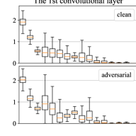
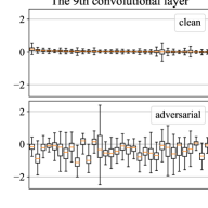
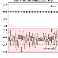
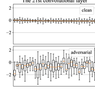
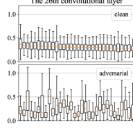
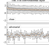
Figure 1: The distribution of 32 most excited channels on average of convolutional layers in a naturally trained WideResNet-32-10 when being shown CIFAR-10 “airplane” images. We compare that against the corresponding channel activations under adversarial “airplane” examples with LPGD-10. Attacking the 17^th layer (shaded in red) resulted in scrambled features across the entire model and incorrect final model outputs.

Figure 2: We used LPGD-100, or PGD with 100 iterations to attack only the $n$^th residual block of a “robust” model. Except the 0^th denotes the output layer and PGD is used. To our surprise, adversaries generated by attacking an early layer are highly transferable to the final classification output of the model. Defending models are respectively obtained from [4, 62, 63, 28, 27, 38, 23].

2 Preliminaries & Related Work

2.1 Adversarial examples

Before one can generate adversarial examples and defend against them, it is necessary to formalize the notion of adversarial examples. We start by defining the classifier model as a function $f_{\bm{\theta}}(\mathbf{x})$, where ${\bm{\theta}}$ is the model parameters, $f_{\bm{\theta}}\colon\mathcal{I}\to\mathbb{R}^{K}$ maps the input image to its classification result, $\mathcal{I}\subset\mathbb{R}^{{C}\times{H}\times{W}}$ limits the image data to a valid range, with $C$ being the number of channels in the image (typically 3 channels for a colored input), $H$ and $W$ the height and width of the image respectively, and $K$ is the number of classes from the model output.

The attacker’s objective is to find an adversarial example $\hat{\mathbf{x}}\in\mathcal{I}$ of the model under attack $f_{\bm{\theta}}$ by (approximately) solving the optimization problem:

$$\max_{\mathclap{\hat{\mathbf{x}}\in\mathcal{I}\wedge\operatorname{d}\left({\mathbf{x}},{\hat{\mathbf{x}}}\right)\leq\epsilon}}\,\operatorname{\mathcal{L}^{\mathrm{sce}}}\left(f_{\bm{\theta}}\left(\hat{\mathbf{x}}\right),\mathbf{y}\right),$$ (1)

where $\operatorname{\mathcal{L}^{\mathrm{sce}}}\left(f_{\bm{\theta}}\left(\hat{\mathbf{x}}\right),\mathbf{y}\right)$ is the softmax cross-entropy (SCE) loss between the output and the one-hot ground truth $\mathbf{y}$. By maximizing the loss, one may arrive at a $\hat{\mathbf{x}}$ such that $\arg\max f_{\bm{\theta}}(\hat{\mathbf{x}})\neq\arg\max\mathbf{y}$. In other words, the model can generally be fooled to produce an incorrect classification. To confine the perturbation, $\operatorname{d}\left({\mathbf{x}},{\hat{\mathbf{x}}}\right)\leq\epsilon$ constrains the distance between the original $\mathbf{x}$ and the adversarial $\hat{\mathbf{x}}$ to be less than or equal some small constant $\epsilon$.

In general, the distance metric $\operatorname{d}\left({\mathbf{x}},{\hat{\mathbf{x}}}\right)$ is commonly defined as the $\ell_{p}$-norm of the difference between $\mathbf{x}$ and $\hat{\mathbf{x}}$ [51, 19, 35, 7]. Different choices of norm were explored in literature,  one pixel attacks [50] minimizes the $\ell_{0}$-norm ${{\|\mathbf{x}-\hat{\mathbf{x}}\|}_{0}}$, while others may be interested in the standard Euclidean distance, the $\ell_{2}$-norm [51, 37, 8]. In this paper, we focus on another popular choice of distance metric, the $\ell_{\infty}$-norm $\operatorname{d}\left({\mathbf{x}},{\hat{\mathbf{x}}}\right)\triangleq{\|\mathbf{x}-\hat{\mathbf{x}}\|}_{\infty}$, as used in [19, 35].

The white-box scenario completely exposes to the attacker to the inner mechanisms of the defense,  the model architecture, its parameters, training data and algorithms, and are revealed to the attacker. The optimal solution of (1), however, is generally unattainable. In practice, approximate solution are instead sought after, often with gradient-based methods,  one of the popular attack method used by defenders for evaluating white-box adversarial robustness is the projected gradient descent (PGD). PGD finds an adversarial example by performing the iterative update [35]:

$$\hat{\mathbf{x}}_{i+1}=\operatorname{\mathcal{P}_{\epsilon,\mathbf{x}}}\left(\hat{\mathbf{x}}_{i}+\alpha_{i}\operatorname{\mathrm{sign}}\left(\nabla_{\hat{\mathbf{x}}_{i}}\operatorname{\mathcal{L}^{\mathrm{sce}}}\left(f_{\bm{\theta}}(\hat{\mathbf{x}}_{i}),\mathbf{y}\right)\right)\right).$$ (2)

Initially, $\hat{\mathbf{x}}_{0}=\operatorname{\mathcal{P}_{\epsilon,\mathbf{x}}}(\mathbf{x}+\mathbf{u})$, where $\mathbf{u}\sim\mathcal{U}\left({[-\epsilon,\epsilon]}\right)$,  $\mathbf{u}$ is a uniform random noise bounded by $[-\epsilon,\epsilon]$. The function $\operatorname{\mathcal{P}_{\epsilon,\mathbf{x}}}\colon\mathbb{R}^{{C}\times{H}\times{W}}\to\mathcal{I}$ clips the range of its input into the $\epsilon$-ball neighbor and the $\mathcal{I}$. The term $\nabla_{\hat{\mathbf{x}}_{i}}\operatorname{\mathcal{L}^{\mathrm{sce}}}\left(f_{\bm{\theta}}(\hat{\mathbf{x}}_{i}),\mathbf{y}\right)$ computes the gradient of the loss the input $\hat{\mathbf{x}}_{i}$. Finally, $\alpha_{i}$ is the step size, and for each element in the tensor $\mathbf{z}$, $\operatorname{\mathrm{sign}}(\mathbf{z})$ returns one of $1$, $0$ or $-1$, if the value is positive, zero or negative respectively. For simplicity, we define:

$$\operatorname{\mathrm{PGD}_{\epsilon,\mathbf{x},\mathbf{y}}}(\mathcal{L},\bm{\alpha},i)\triangleq\hat{\mathbf{x}}_{i},$$ (3)

the result of iterating for $i$ times with a sequence of step sizes $\bm{\alpha}$ and the loss function $\mathcal{L}$ on the original image $\mathbf{x}$. Other gradient-based methods include fast gradient-sign method (FGSM) [19], basic iterative method (BIM) [31], momentum iterative method (MIM) [16] and fast adaptive boundary attack (FAB) [13] for $\ell_{\infty}$-norm attacks, Carlini and Wagner (C&W) [8] for $\ell_{2}$-norm attacks, and DeepFool [37] for both. Similar to PGD, they only iteratively leverage the loss gradient $\nabla_{\hat{\mathbf{x}}_{i}}\mathcal{L}\left(f_{\bm{\theta}}(\hat{\mathbf{x}}_{i}),\cdots\right)$, as all of them adopt a holistic view on the model $f_{\bm{\theta}}$.

Because the SCE loss function $\operatorname{\mathcal{L}^{\mathrm{sce}}}$ in the objective (1) is highly non-linear, easily saturated, and normally evaluated with limited floating-point precision, gradient-based attacks may experience vanishing gradients and difficulty converging [8, 14]. Recent attack methods hence use surrogate losses instead for gradient calculation [8, 21], and optimize an alternative objective by replacing $\operatorname{\mathcal{L}^{\mathrm{sce}}}$ with a custom surrogate loss function. As the alternative objective is usually aligned with the original, maximizing the latter would also maximize the former.

Many auxiliary tricks can push the limit of existing attack methods, for instance, a step-size schedule [14, 21] with a decaying step-size in relation to the iteration count could improve the overall success rate. Multi-targeted attack [21, 44, 43] uses label-specific surrogate loss by enumerating all possible target labels. Attackers may also resort to an ensemble of multiple attack strategies, making the compound approach stronger than any individual attacks [7, 14]. The latter two methods, however, tend to introduce an order of magnitude increase in the worse-case computational costs.

Generative networks that learn from the loss were proposed for adversarial example synthesis [5, 26]. This tactic can be further enhanced with generative adversarial networks (GANs) [18], where the discriminator network encourages the distribution of adversarial examples to become indistinguishable from that of natural examples [59, 36].

Finally, there are a few recent publications that leverages latent features in their attacks [30, 41]. Unlike these methods, considers $\ell_{\infty}$-norm white-box attacks, and further differentiate itself from them as it learns to attack defending models.

2.2 Defending against adversarial examples

The objective of robustness against adversarial examples can be formalized as a saddle point problem, which finds model parameters that minimize the adversarial loss [35]:

$$\min_{\bm{\theta}}\mathsf{E}_{(\mathbf{x},\mathbf{y})\sim\mathcal{D}_{\mathrm{train}}}\left[{\qquad\!\max_{\mathclap{\hat{\mathbf{x}}\in\mathcal{I}\wedge\operatorname{d}\left({\mathbf{x}},{\hat{\mathbf{x}}}\right)\leq\epsilon}}\,\operatorname{\mathcal{L}^{\mathrm{sce}}}\left(f_{\bm{\theta}}\left(\hat{\mathbf{x}}\right),\mathbf{y}\right)}\right],$$ (4)

where $\mathcal{D}_{\mathrm{train}}$ contains pairs of input images $\mathbf{x}$ and ground truth labels $\mathbf{y}$. A straightforward approach to approximately solving the above objective (4) is via adversarial training [32], which trains the model with adversarial examples computed on-the-fly using, for instance, PGD [35].

Figure 3: High-level overview of . Note that in each of the steps, layers in (gray) regions remain fixed, (dotted outline) regions denote new layers added by , (green) layers are being trained, and losses in (cyan) and (red) blocks are respectively minimized and maximized. (a) illustrates the original pre-trained model, where ${f}^{\scriptscriptstyle({l})}$ denotes the $l$^th layer (or residual block). (b) trains additional fully-connected layers from intermediate layers, each with a softmax cross-entropy loss until convergence. (c) computes adversarial examples iteratively with a weighted sum of surrogate losses. (d) uses the adversarial examples from (c) to evaluate the robustness of the original model.

Many adversarial defense strategies follow the same paradigm, but train the model with different loss objective functions in order to further foster robustness. Along with the standard classification loss, TRADES [64] minimizes the multi-class calibrated loss between the output of the original image and the one of the adversarial example. Misclassification-aware regularization [55] encourages the smoothness of the network output, even when it produces misclassified results. Self-adaptive training [24] allows the training algorithm to adapt to noise added to the training data. Feature scattering [62] generates adversarial examples for training by maximizing the distances between features extracted from the natural and adversarial examples. Neural level-sets [4] and sensible adversarial training [28] use different proxy robustness objectives for adversarial training. Hypersphere embedding [43] normalizes weights and features to be on the surface of hyperspheres, and also normalizes the angular margin of the logits layer. Prototype conformity loss [38], and manifold regularization [27] adopt different regularization losses to allow the model to learn a smooth loss landscape changes in $\mathbf{x}$. Stylized adversarial defense [39] and learning-to-learn (L2L) [26] propose to use neural networks to generate adversarial examples for training. Finally, self-training with unlabeled data [9, 2] can substantially improve robustness in a way that cannot be trivially broken by adversarial attacks.

As robust models may be substantially larger than non-robust ones, there have been a recent interest in making them more space and time efficient. Alternating direction method of multipliers (ADMM) has been applied to prune and adversarial train CNNs jointly [60]. HYDRA [47] preserves the robustness of pruned models by integrating the pruning objective into the adversarial loss optimization.

Adversarial training often requires several iterations to compute adversarial examples for each model parameter update, which is multiple times more expensive than traditional training with natural examples. Adversarial training for free [48] address this problem by interleaving adversary updates with model updates for efficient training of robust CNNs. Fast adversarial training [56] further accelerates the training by using a simpler FGSM-based adversary.

Finally, others provide practical considerations and tricks for stronger adversarial defense [7, 42, 46, 57, 11].

3 The Method

We introduce by providing a high-level illustration (Figure 3) of its attack procedure. First, for a firm grip on latent features, it starts by training fully-connected layers for each residual block with the training set until convergence. Note that we ensure the original model $f_{\bm{\theta}}$ to remain constant during this process. To compute adversarial examples, we maximize the alternative adversarial loss $\hat{L}$, which is an adaptively-weighted sum of surrogate losses from individual layers. For testing of adversarial robustness, the generated adversarial example is then transferred to the original model $f_{\bm{\theta}}$ for evaluation.

3.1 Latent feature adversarial

Following the footsteps of surrogate losses, in Section 1 we postulate that a similarly indirect loss on latent features can also effectively enhance adversarial attacks. exploits the features extracted from intermediate layers to craft even stronger adversarial examples for $f_{\bm{\theta}}$. We assume the model architecture $f_{\bm{\theta}}$ to generally comprise a sequence of $N$ layers (or residual blocks) and can be represented as:

$$f_{\bm{\theta}}(\mathbf{x})={f}^{\scriptscriptstyle({N})}(\cdots{f}^{\scriptscriptstyle({2})}({f}^{\scriptscriptstyle({1})}(\mathbf{x}))\cdots),$$ (5)

where ${f}^{\scriptscriptstyle({1})},{f}^{\scriptscriptstyle({2})},\ldots,{f}^{\scriptscriptstyle({N})}$ denotes the sequence of intermediate layers in the model. For simplicity in notation, we omit the parameters from individual layers. We therefore formalize this proposal by generalizing the traditional PGD attack (2) with a latent-feature PGD (LFPGD) adversarial optimization problem:

$$\max_{\mathclap{\bm{h},\,\bm{\lambda},\,\bm{\alpha},\,\operatorname{\mathcal{L}^{\mathrm{sur}}}}}\quad\,\operatorname{\mathcal{L}^{\mathrm{sce}}}\!\left(f_{\bm{\theta}}\left(\operatorname{\mathrm{PGD}_{\epsilon,\mathbf{x},\mathbf{y}}}\left(\operatorname{\mathcal{L}^{\mathrm{lf}}_{\bm{\lambda}}},\bm{\alpha},I\right)\right),\mathbf{y}\right),$$ (6)

where $$\operatorname{\mathcal{L}^{\mathrm{lf}}_{\bm{\lambda}}}(\mathbf{z})=\operatorname{\mathcal{L}^{\mathrm{sur}}}\!\left({\textstyle\sum_{l\in[1:N]}}{\lambda}^{\scriptscriptstyle({l})}{h}^{\scriptscriptstyle({l})}\left({\mathbf{z}}^{\scriptscriptstyle({l})}\right),\mathbf{y}\right).$$

Here, the constant $I$ is the maximum number of gradient-update iterations. For each layer $l\in{[1:N]}$, ${\lambda}^{\scriptscriptstyle({l})}\in[0,1]$ assigns an importance value to the layer gradient with $\sum_{l\in N}{\lambda}^{\scriptscriptstyle({l})}=1$. The term ${\mathbf{z}}^{\scriptscriptstyle({l})}\triangleq{f}^{\scriptscriptstyle({l})}\circ\cdots\circ{f}^{\scriptscriptstyle({1})}(\mathbf{z})$ denotes the feature extracted from the $l$^th layer, The function ${h}^{\scriptscriptstyle({l})}$ for the $l$^th layer maps the features from ${f}^{\scriptscriptstyle({l})}$ to logits. Finally, $\alpha_{i}$ is a step-size schedule. Our goal is hence to find the right combinations of logits functions $\bm{h}\triangleq({h}^{\scriptscriptstyle({1})},\ldots,{h}^{\scriptscriptstyle({N})})$ and their corresponding weights $\bm{\lambda}\triangleq({\lambda}^{\scriptscriptstyle({1})},\ldots,{\lambda}^{\scriptscriptstyle({N})})$ from intermediate layers, the step-size schedule $\bm{\alpha}$, and the surrogate loss $\operatorname{\mathcal{L}^{\mathrm{sur}}}$ to use.

Solving the LFPGD optimization is unfortunately infeasible in practice. For which we devise methods that could approximately solve it, and nevertheless enable us to generate adversarial examples stronger than competing methods.

3.2 Training intermediate logits layers

To utilize latent features, we begin by training logits layers ${h}^{\scriptscriptstyle({l})}$ for individual intermediate layers ${f}^{\scriptscriptstyle({l})}$ for all $l\in[1:N-1]$ with conventional stochastic gradient descent (SGD) until convergence. The function ${h}^{\scriptscriptstyle({l})}\colon\mathbb{R}^{{C}^{\scriptscriptstyle({l})}\times{H}^{\scriptscriptstyle({l})}\times{W}^{\scriptscriptstyle({l})}}\to\mathbb{R}^{K}$ is defined as a small auxiliary classifier composed of a global average pooling layer $\operatorname{\mathrm{pool}}\colon\mathbb{R}^{{C}^{\scriptscriptstyle({l})}\times{H}^{\scriptscriptstyle({l})}\times{W}^{\scriptscriptstyle({l})}}\to\mathbb{R}^{{C}^{\scriptscriptstyle({l})}}$ followed by a fully-connected layer for classification:

$${h}^{\scriptscriptstyle({l})}({\mathbf{x}}^{\scriptscriptstyle({l})})\triangleq\operatorname{\mathrm{pool}}\left({\mathbf{x}}^{\scriptscriptstyle({l})}\right){\bm{\phi}}^{\scriptscriptstyle({l})}+{\bm{\eta}}^{\scriptscriptstyle({l})},$$ (7)

where ${\mathbf{x}}^{\scriptscriptstyle({l})}$ denotes the features extracted from the $l$^th layer, ${\bm{\phi}}^{\scriptscriptstyle({l})}\in\mathbb{R}^{{C}^{\scriptscriptstyle({l})}\times K}$ and ${\bm{\eta}}^{\scriptscriptstyle({l})}\in\mathbb{R}^{K}$ are parameters to be trained in the function ${h}^{\scriptscriptstyle({l})}$. As the final layer ${f}^{\scriptscriptstyle({N})}$ is already a logits layer, we assume ${h}^{\scriptscriptstyle({N})}\triangleq\mathrm{id}$ is an identity function.

Depending on the availability, we could train the added layers with either $\mathcal{D}_{\mathrm{train}}$, the data samples used for attack $\mathcal{D}_{\mathrm{attack}}$, or both together. While we used $\mathcal{D}_{\mathrm{train}}$ in our experiments, we observed in practice negligible differences in either attack strengths given sufficient amount of training examples, as they are theoretically drawn from the same data sampling distribution.

It is important to note that during the training procedure of ${h}^{\scriptscriptstyle({l})}$, the original model $f_{\bm{\theta}}$ is used as a feature extractor, with all training techniques ( dropout, parameter update, ) disabled. This means that the model parameters ${\bm{\theta}}$, the layers $f_{l}$, and their parameters, batch normalization [25] statistics, and remain constant, while only the parameters in ${h}^{\scriptscriptstyle({l})}$ functions are being trained.

3.3 Choosing intermediate layers to attack

The search space for ${\lambda}^{\scriptscriptstyle({1:N})}$ is difficult to navigate because of the computations cost associated with finding a statistically significant amount of adversarial examples. For this reason, simplifies the search with a greedy yet effective process. First, we enumerate over all intermediate layers $l\in[1:N-1]$, and let

$$\operatorname{\mathcal{L}^{\mathrm{lf}}_{\bm{\lambda}}}(\mathbf{z},\mathbf{y})=\operatorname{\mathcal{L}^{\mathrm{sur}}}\left({\textstyle\beta{h}^{\scriptscriptstyle({l})}\!\left({\mathbf{z}}^{\scriptscriptstyle({l})}\right)+(1-\beta)f_{\bm{\theta}}(\mathbf{z}),\mathbf{y}}\right)$$ (8)

by setting $\bm{\lambda}=\beta\operatorname{\mathrm{onehot}}(N,N)+(1-\beta)\operatorname{\mathrm{onehot}}(l,N),$ where initially $\beta=\frac{1}{2}$. In other words, the attack is now using only the $l$^th layer together with the output layer at a time while disabling all others. With this method, we can discover the most effective layer for subsequent attack procedures across all images in $\mathcal{D}_{\mathrm{attack}}$. Empirically, we found in most defending models the weakest link is the penultimate residual block, and this search procedure can thus be skipped entirely for performance considerations. There are, however, exceptions: for instance, we found in the model from [38], the 6^th last residual block exhibits the weakest defense and attacks using it converge faster.

Finally, empirical results revealed that the intermediate layer $l$ can be adaptively disabled if it misclassifies the adversarial example,  when $\arg\max{h}^{\scriptscriptstyle({l})}(\hat{\mathbf{x}}_{i})\neq\mathbf{y}$, in order to optimize faster towards the original adversarial objective (1). We incorporate this in the final algorithm.

3.4 Surrogate loss function

Gradients computed from the SCE loss has been notoriously shown to easily underflow in floating-point arithmetic [8, 14]. For this reason, surrogate loss functions have been proposed [8, 21, 14] to work around this limitation. Despite their effectiveness in breaking through defenses, it is difficult to interpret why they work as they are no longer maximize the original adversarial objective (1) directly. As a result, we propose a small modification to the original SCE loss, which scales the logits adaptively before evaluating the softmax operation:

$$\operatorname{\mathcal{L}^{\mathrm{sur}}}(\mathbf{z},\mathbf{y})\triangleq\operatorname{\mathcal{L}^{\mathrm{sce}}}\!\left(\frac{\mathbf{z}}{t}{\left(\mathbf{y}^{\top}\mathbf{z}-\max\left(\left(1-\mathbf{y}\right)\cdot\mathbf{z}\right)\right)}^{-1},\mathbf{y}\right),$$ (9)

where $\cdot$ denotes the element-wise product, and the temperature $t=1$ in all of our experiments. Here, $\mathbf{y}^{\top}\mathbf{z}-\max\left({\left(1-\mathbf{y}\right)}\cdot\mathbf{z}\right)$ is known as the difference of logits (DL) [8], which evaluates the difference between the largest output in the logits $\mathbf{z}$ against the second largest. The negated version of DL and the ratio-based variant—the difference of the logits ratio (DLR) loss—have respectively been used as surrogate losses in [8] and [14].

Our surrogate loss (9) has twofold advantages. First, it prevents the gradients from floating-point underflows and improves convergence. Second, unlike the DL or the DLR loss, it can still represent the original SCE loss in a faithful fashion, and all logits can still contribute to the final loss.

Finally, we define a targeted variant of $\operatorname{\mathcal{L}^{\mathrm{sur}}}$, which moves the logits towards a predefined target class $k$, with a one-hot vector ${\bm{\tau}}=\operatorname{\mathrm{onehot}}(k,K)$:

$$\operatorname{\mathcal{L}^{\mathrm{sur}}_{\bm{\tau}}}(\mathbf{z},\mathbf{y})\triangleq-\operatorname{\mathcal{L}^{\mathrm{sce}}}\!\left(\frac{\mathbf{z}}{t}{\left(\mathbf{y}^{\top}\mathbf{z}-\max\left(\left(1-\mathbf{y}\right)\cdot\mathbf{z}\right)\right)}^{-1},{\bm{\tau}}\right),$$ (10)

3.5 Summary

In addition to the original contributions explained above, we also employ simple yet helpful tactics from previous literatures. First, a step-size schedule with a linear decay $2\epsilon(1-i/I),$ is used in the iterative updates, where $\epsilon$ is the $\ell_{\infty}$-norm perturbation boundary $\epsilon$ in (1), $i$ is the current iteration number and $I$ denotes the total number of iterations. Second, we adapt momentum-based updates from [14].

To summarize, we illustrate the algorithm in Algorithm 1. The function $\mathtt{\attack\_\,Attack}$ accepts the following inputs: the model $f_{\bm{\theta}}$, the pretrained logits function for the $l$^th layer to be attacked jointly, natural image $\mathbf{x}$ and its one-hot label $\mathbf{y}$, the step-size $\alpha$, the interpolation parameter $\beta$ between the $l$^th layer and the output layer, the momentum weight used $\nu$, the perturbation boundary $\epsilon$, and lastly the maximum iteration count $I$.

With the algorithm above, we can perform a simple grid search on $\beta\in[0,1]$. As using latent features results in faster convergence, the search can start from a point in the middle ( 0.5) to minimize the number of iterations required to attack each image. Finally, to further push the limit of , we could incorporate the multi-targeted attack [21],  after the untargeted surrogate loss (9), we enumerate $k\in[1:K]\,/\arg\max\mathbf{y}$,  all possible target classes except for the ground truth, with the targeted surrogate loss $\operatorname{\mathcal{L}^{\mathrm{sur}}_{\bm{\tau}}}$ defined in (10). For computational efficiency, the above search procedure can be early-stopped for successful adversarial examples, until all images in $\mathcal{D}_{\mathrm{attack}}$ have been sift through progressively.

4 Experiments

For a fair comparison against existing work on adversarial attacks across different defense techniques, in our evaluation we used the most common $\ell_{\infty}$-norm threat model on the CIFAR-10 and CIFAR-100 datasets [29]. We extracted from recent publications with open PyTorch defense models for testing, and ensured the list to be as comprehensive as possible. We reproduced traditional white-box attacks (PGD [35], BIM [31], MIM [16], FAB [13]), all with 100 iterations and a constant step-size of $2/255$ as baselines. We use LAF${}^{\text{\,{MT}}}_{\text{$I,B$}}$ to denote flavors of , where $I$ is the number of gradient iterations used, $B$ is the number of $\beta$ values searched, and MT denotes the use of multi-targets. The CIFAR-10 testing set is assumed to be $\mathcal{D}_{\mathrm{attack}}$, and the momentum of the iterative updates is $\nu=0.75$. A full comparison can be found in Table 1. It reveals that not only is LAF${}^{\text{\,{MT}}}_{\text{100,6}}$ an even stronger attack than AutoAttack (AA) [14], the current SOTA in the robustness evaluation of defense strategies, but also it has a better worst-case complexity in terms of the maximum number of forward-passes required for each image. To push the boundary of , we also report LAF${}^{\text{\,{MT}}}_{\text{1\,\text{k},10}}$, which enjoys a substantial increase in compute effort. Note that AA as an ensemble combines multiple strategies (PGD with momentum and two surrogate losses [14], square attack [3] and FAB [13]), whereas uses only Algorithm 1 uniformly.

Algorithm 1 The white-box attack.

1:function _ Attack($f_{\bm{\theta}},{h}^{\scriptscriptstyle({l})},\mathbf{x},\mathbf{y},\alpha,\beta,\nu,\epsilon,I$)

2:     $\hat{\mathbf{x}}_{0}\leftarrow\operatorname{\mathcal{P}_{\epsilon,\mathbf{x}}}\left(\mathbf{x}+\mathbf{u}\right)$, $\triangleright$ Optional random start

3:      $\hat{\mathbf{x}}_{0}\leftarrow\!$ where $\mathbf{u}\sim\mathcal{U}\left({[-\epsilon,\epsilon]}\right)$

4:     $\bm{\mu}_{0}\leftarrow 0$

5:     for $i\in[0:I-1]$ do

6:         $\mathbf{z}_{o}\leftarrow f_{\bm{\theta}}(\hat{\mathbf{x}}_{i})$,  $\mathbf{z}_{l}\leftarrow{h}^{\scriptscriptstyle({l})}({f}^{\scriptscriptstyle({l})}(\hat{\mathbf{x}}_{i}))$

7:         $\sigma_{o}\leftarrow\mathbf{y}^{\top}\mathbf{z}_{o}-\max\left(\left(1-\mathbf{y}\right)\cdot\mathbf{z}_{o}\right)$

8:         if $\sigma_{o}\leq 0$ then return $\hat{\mathbf{x}}_{i}$ $\triangleright$ Successful attack

9:         $\sigma_{l}\leftarrow\mathbf{y}^{\top}\mathbf{z}_{l}-\max\left(\left(1-\mathbf{y}\right)\cdot\mathbf{z}_{l}\right)$

10:         $\beta_{i}\leftarrow 1$ if $\sigma_{l}\leq 0$ else $\beta$ $\triangleright$ Adaptive weight

11:         $\mathbf{z}\leftarrow\beta_{i}\frac{\mathbf{z}_{o}}{\sigma_{o}}+(1-\beta_{i})\frac{\mathbf{z}_{l}}{\sigma_{l}}$ $\triangleright$ Surrogate loss

12:         $\bm{g}_{i+1}\leftarrow\operatorname{\mathrm{sign}}\left(\nabla_{\hat{\mathbf{x}}_{i}}\!\operatorname{\mathcal{L}^{\mathrm{sce}}}\left(\frac{\mathbf{z}}{t},\mathbf{y}\right)\right)$

13:         $\alpha\leftarrow 2\epsilon(1-\frac{i}{I})$ $\triangleright$ Linear step-size schedule

14:         $\bm{\mu}_{i+1}\leftarrow\operatorname{\mathcal{P}_{\epsilon,\mathbf{x}}}\left(\bm{\mu}_{i}+\alpha\bm{g}_{i+1}\right)$ $\triangleright$ Momentum

15:         $\hat{\mathbf{x}}_{i+1}\leftarrow\operatorname{\mathcal{P}_{\epsilon,\mathbf{x}}}\left(\hat{\mathbf{x}}_{i}+{}\right.$ $\triangleright$ Iterative update

16:         $\left.\quad\nu\left(\bm{\mu}_{i+1}-\hat{\mathbf{x}}_{i}\right)+(1-\nu)\left(\hat{\mathbf{x}}_{i}-\hat{\mathbf{x}}_{i-1}\right)\right)$

17:     end for

18:     return $\hat{\mathbf{x}}_{I}$ $\triangleright$ Give up after $I$ iterations

19:end function

Table 1: Comparing accuracy under attack (%) of against iterative methods [35, 31, 16, 13] and AutoAttack (AA₁₀₀) [14] across various defense strategies. The “$\bm{\Delta}$” column shows the difference between the reported (“Nominal”) and accuracies. Models marked with † were additionally trained with unlabeled datasets [53]. We used $\epsilon=8/255$ except for models marked with ‡, which used $\epsilon=0.031$ as originally reported by the authors.

CIFAR-10 defense method Clean Nominal PGD MIM BIM FAB AA₁₀₀ LAF${}^{\text{\,{MT}}}_{\text{100,6}}$ LAF${}^{\text{\,{MT}}}_{\text{1\,\text{k},10}}$ $\bm{\Delta}$ Worst-case complexity 1 100 100 100 100 8.3 k 6 k 100 k Adversarial weight perturbation [58]^† $88.25$ $60.04$ $63.26$ $66.17$ $65.33$ $60.72$ $60.04$ $59.97$ $59.94$ $-0.10$ Unlabeled [9]^† $89.69$ $62.5$ $62.17$ $67.21$ $65.77$ $60.85$ $59.53$ $59.42$ $59.37$ $-3.13$ HYDRA [47]^† $88.98$ $59.98$ $59.98$ $65.29$ $63.87$ $58.33$ $57.14$ $57.02$ $56.98$ $-3.00$ Misclassification-aware [55]^† $87.5$ $65.04$ $62.55$ $66.74$ $65.57$ $57.60$ $56.29$ $56.13$ $56.07$ $-8.97$ Pre-training[22]^† $87.11$ $57.4$ $57.54$ $61.51$ $60.25$ $55.58$ $54.92$ $54.80$ $54.74$ $-2.66$ Hypersphere embedding [43] $85.14$ $62.14$ $62.17$ $63.66$ $63.15$ $54.47$ $53.74$ $53.68$ $53.64$ $-8.50$ Overfitting [46] $85.34$ $58.0$ $57.24$ $60.48$ $59.49$ $54.3$ $53.42$ $53.34$ $53.32$ $-4.68$ Self-adaptive training [24]^‡ $83.48$ $58.03$ $56.58$ $60.07$ $58.89$ $54.52$ $53.33$ $53.19$ $53.19$ $-4.84$ TRADES [64]^‡ $84.92$ $56.43$ $55.50$ $59.16$ $58.06$ $53.96$ $53.08$ $52.98$ $52.94$ $-3.49$ Robustness (Python Library) [17] $87.03$ $53.29$ $52.32$ $58.39$ $56.52$ $50.67$ $49.21$ $49.11$ $49.09$ $-4.20$ YOPO [61] $87.20$ $47.98$ $46.15$ $52.57$ $50.69$ $45.80$ $44.83$ $44.73$ $44.71$ $-1.44$ Fast adversarial training [56] $83.8$ $46.44$ $46.44$ $52.02$ $50.53$ $44.52$ $43.41$ $43.29$ $43.27$ $-3.17$ MMA training [15] $83.28$ $47.18$ $47.29$ $56.44$ $54.65$ $46.88$ $40.21$ $39.84$ $39.74$ $-7.44$ Neural level sets [4]^‡ $81.3$ $79.67$ $79.83$ $79.83$ $79.83$ $40.98$ $40.22$ $39.81$ $39.77$ $-39.90$ Feature scattering [62] $89.98$ $60.6$ $69.01$ $75.66$ $74.54$ $43.42$ $36.64$ $36.02$ $35.94$ $-24.66$ Adversarial interpolation [63] $90.25$ $68.7$ $73.13$ $75.84$ $74.95$ $43.34$ $36.45$ $35.24$ $35.14$ $-33.56$ Sensible adversarial training [28] $91.51$ $57.23$ $59.93$ $68.79$ $66.85$ $41.87$ $34.22$ $33.39$ $33.33$ $-23.90$ Stylized adversarial defense [39] $93.29$ $78.68$ $78.68$ $82.87$ $82.50$ $19.14$ $13.42$ $11.16$ $11.09$ $-67.59$ Manifold regularization [27] $90.84$ $77.68$ $77.68$ $77.63$ $77.30$ $27.18$ $1.35$ $0.22$ $0.21$ $-77.47$ Polytope conformity loss [38] $89.16$ $32.32$ $19.42$ $42.88$ $38.77$ $5.81$ $0.28$ $0.06$ $0.03$ $-32.29$ CIFAR-100 defense method Clean Nominal PGD MIM BIM FAB AA₁₀₀ LAF${}^{\text{\,{MT}}}_{\text{100,6}}$ LAF${}^{\text{\,{MT}}}_{\text{1\,\text{k},10}}$ $\bm{\Delta}$ Worst-case complexity 1 100 100 100 100 8.3 k 6 k 100 k Adversarial weight perturbation [58] $60.38$ $28.86$ $33.68$ $35.24$ $34.70$ $29.25$ $28.86$ $28.79$ $28.77$ $-0.09$ Pre-training [22]^† $59.23$ $33.5$ $33.70$ $35.66$ $35.09$ $28.83$ $28.42$ $28.25$ $28.23$ $-5.27$ Progressive Hardening [49] $62.82$ $24.57$ $26.75$ $30.78$ $29.66$ $25.14$ $24.57$ $24.50$ $24.48$ $-0.09$ Overfitting [46] $53.83$ $28.1$ $20.95$ $24.0$ $23.10$ $19.49$ $18.95$ $18.87$ $18.86$ $-9.24$

Faster convergence. It is sensible to argue that models could also rely on computational security as one of their defense tactics. We would like to highlight that in contrast to most attack methods, the effectiveness of is not accompanied by high computational costs. We found that by exploiting latent features, it generally leads to faster convergences to adversarial examples than competing methods. In Figure 4, we compare the speed of convergence among three different methods. For baseline, we used PGD-1000. We picked APGD_DLR with 100 iterations and 10 restarts, the most effective attack method of the AA ensemble [14] across most defense methods in Table 1. For computational fairness, we selected LAF${}^{\text{\,{}}}_{\text{100,10}}$ to compete against it, which is an untargeted with a 10-valued $\beta\in\{0.0,0.1,0.2,\ldots,0.9\}$ grid search starting from $0.5$, where each value used only 100 iterations. The results show that for all 4 defending models, is not only stronger, but also often orders of magnitude faster than APGD_DLR and PGD for successful attacks. Finally, the logits layers introduce minuscule overhead ($\leq\!\!{0.008\%}$ in all models), and have no discernible impact on the iteration time.

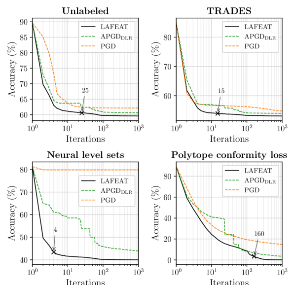
Figure 4: Comparing the performance of LAF${}^{\text{\,{}}}_{\text{100,10}}$ against other adversarial attack methods (APGD_DLR [14] and PGD [35]) on defenders [9, 64, 4, 38]. The horizontal and vertical axes respectively show the number of iterations used so far, and the percentage of remaining unsuccessful examples. The iteration count needed for to defeat APGD_DLR-100 (10 restarts) is also marked.

Adversarial-trained latent features improve model robustness. As demonstrated earlier with , one can exploit the latent features learned by defending models to craft powerful adversarial examples. A question then ensues: is it possible to fortify latent features against attacks to improve model robustness? To answer this, we carried out a simple experiment and trained two WideResNet-32-10 models, both with ordinary PGD-7 adversarial training from [35]. The only difference is that in one of them we additionally introduced logits layers for residual block outputs to be adversarial trained along with the output layer. For attacks, we likewise ablated with the use of latent features. The results can be found in Table 2. Note that the model with robust latent features displayed a better defense against all attacks than the other. Even when faced against attacks that do no leverage latent features, Perhaps the most revealing result is: training latent features to be more robust can improve the overall robustness even when faced against attacks without using latent features.

Table 2: PGD-7 adversarial training LAF${}^{\text{\,{}}}_{\text{100,10}}$, both explored with (+LF) and without (–LF) latent features.

Accuracy under			Adversarial Attack
attack (%)		Clean	PGD-100	–LF	+LF
Defense	–LF	79.56	47.06	41.21	41.05
	+LF	83.53	47.17	41.50	41.26

Compression robustness. In Table 3, compressed models from HYDRA [47] displayed a worsening robustness degradation between the reported (PGD-50 with 10 restarts) and LAF${}^{\text{\,{}}}_{\text{100,10}}$ for an increasing pruning ratio. This shows that model-holistic attacks can potentially overestimate the robustness of compressed models.

Table 3: The effect of LAF${}^{\text{\,{}}}_{\text{100}}$ on the adversarial trained and compressed WideResNet-28-4 models from HYDRA [47]. PR denotes pruning ratio,  the percentage of zeros in model weights.

PR (%)	Clean	Nominal		$\bm{\Delta}$
0%	$85.6$	$57.2$	$53.94$	$-3.26$
90%	$83.7$	$55.2$	$51.68$	$-3.52$
95%	$82.7$	$54.2$	$49.87$	$-4.33$
99%	$75.6$	$47.3$	$42.73$	$-4.57$

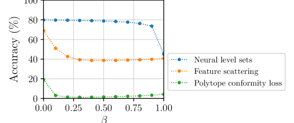
Figure 5: Accuracy under attack $\beta$, the interpolation between the output and latent logits for [4, 62, 38], Here, $\beta=0$ uses only the output logits, and $1$ uses only the latent logits.

Interpolation between latent and output logits. Figure 5 varies the weight between the most effective latent feature and the final logits output for LAF${}^{\text{\,{}}}_{\text{100,10}}$. It used $\beta\in\{0.0,0.1,\ldots,0.9\}$ and 100 iterations for each. The result showed that different defense strategies call for distinct $\beta$ values, making the search of $\beta$ a compelling necessity.

Ablation analysis. Figure 6 performs ablation analysis of 4 tactics employed by across 14 defending models, where 3 were introduced in this paper,  the use of latent features, a new surrogate loss, and a linear decay step-size schedule. The last one is the multi-targeted attack inspired by [21]. Across all 16 combinations of them, we discovered that adding latent features to an existing combination of methods always brings the greatest accuracy impact among possible choices.

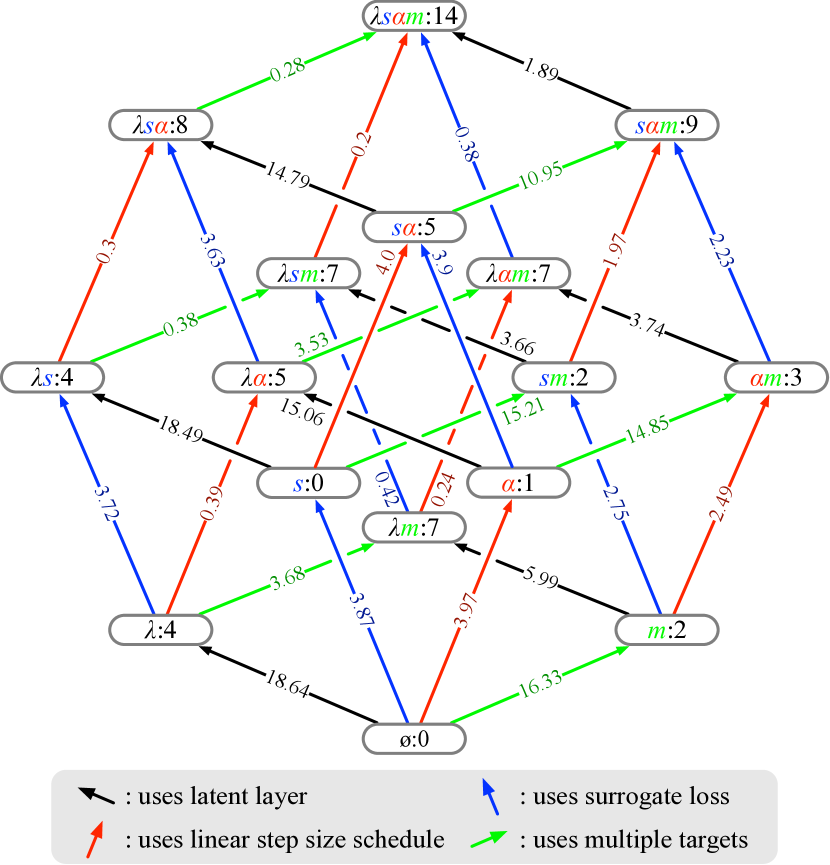
Figure 6: We ablate the full LAF${}^{\text{\,{MT}}}_{\text{100}}$ of its 4 tactics on a complete lattice. Here, each node is a unique combination of 4 tactics, where $\color[rgb]{0,0,0}$ uses a latent layer with $\beta$ search; $\color[rgb]{0,0,1}{s}$ is the surrogate loss instead of the standard SCE loss; $\color[rgb]{1,0,0}{\alpha}$ uses the linear step-size schedule; and $\color[rgb]{0,1,0}{m}$ denotes multiple targets, and the number indicates the number of methods where is better than AA across 14 different defenses [9, 47, 55, 22, 23, 64, 56, 4, 62, 63, 28, 27, 38, 39]. The arrows , , and represent the introduction of the corresponding tactics, and each number on an arrow indicates the average accuracy degradation as a result of adding that tactic.

5 Conclusion

demonstrated that exploiting latent features is highly effective against many recent defense techniques. It efficiently outperformed the current SOTA attack methods across a wide-range of defenses. We believe that the future progress of adversarial attack and defense on CNNs depends on the understanding of how latent features can be effectively used as novel attack vectors. The evaluation of adversarial robustness, therefore, cannot view the model from a holistic perspective. We made open-source and hope it could pave the way for gaining knowledge on robustness evaluation from the explicit use of latent features.

References

- [1] Samet Akçay, Mikolaj E Kundegorski, Michael Devereux, and Toby P Breckon. Transfer learning using convolutional neural networks for object classification within X-ray baggage security imagery. In 2016 IEEE International Conference on Image Processing (ICIP), pages 1057–1061. IEEE, 2016.
- [2] Jean-Baptiste Alayrac, Jonathan Uesato, Po-Sen Huang, Alhussein Fawzi, Robert Stanforth, and Pushmeet Kohli. Are labels required for improving adversarial robustness? In Advances in Neural Information Processing Systems, volume 32, 2019.
- [3] Maksym Andriushchenko, Francesco Croce, Nicolas Flammarion, and Matthias Hein. Square attack: a query-efficient black-box adversarial attack via random search. In ECCV, 2020.
- [4] Matan Atzmon, Niv Haim, Lior Yariv, Ofer Israelov, Haggai Maron, and Yaron Lipman. Controlling neural level sets. In Advances in Neural Information Processing Systems, pages 2032–2041, 2019.
- [5] Shumeet Baluja and Ian Fischer. Learning to attack: Adversarial transformation networks. In Thirty-second aaai conference on artificial intelligence, 2018.
- [6] Mariusz Bojarski, Anna Choromanska, Krzysztof Choromanski, Bernhard Firner, Larry J Ackel, Urs Muller, Phil Yeres, and Karol Zieba. Visualbackprop: Efficient visualization of cnns for autonomous driving. In 2018 IEEE International Conference on Robotics and Automation (ICRA), pages 1–8. IEEE, 2018.
- [7] Nicholas Carlini, Anish Athalye, Nicolas Papernot, Wieland Brendel, Jonas Rauber, Dimitris Tsipras, Ian Goodfellow, Aleksander Madry, and Alexey Kurakin. On evaluating adversarial robustness. arXiv preprint arXiv:1902.06705, 2019.
- [8] N. Carlini and D. Wagner. Towards evaluating the robustness of neural networks. In 2017 IEEE Symposium on Security and Privacy (SP), pages 39–57, 2017.
- [9] Yair Carmon, Aditi Raghunathan, Ludwig Schmidt, John C Duchi, and Percy S Liang. Unlabeled data improves adversarial robustness. In Advances in Neural Information Processing Systems, volume 32, pages 11192–11203, 2019.
- [10] Shan Carter, Zan Armstrong, Ludwig Schubert, Ian Johnson, and Chris Olah. Activation atlas. Distill, 2019. https://distill.pub/2019/activation-atlas.
- [11] Tianlong Chen, Sijia Liu, Shiyu Chang, Yu Cheng, Lisa Amini, and Zhangyang Wang. Adversarial robustness: From self-supervised pre-training to fine-tuning. In Proceedings of the IEEE/CVF Conference on Computer Vision and Pattern Recognition (CVPR), June 2020.
- [12] Taoran Cheng, Pengcheng Wen, and Yang Li. Research status of artificial neural network and its application assumption in aviation. In 2016 12th International Conference on Computational Intelligence and Security (CIS), pages 407–410. IEEE, 2016.
- [13] Francesco Croce and Matthias Hein. Minimally distorted adversarial examples with a fast adaptive boundary attack. In ICML, 2020.
- [14] Francesco Croce and Matthias Hein. Reliable evaluation of adversarial robustness with an ensemble of diverse parameter-free attacks. In ICML, 2020.
- [15] Gavin Weiguang Ding, Yash Sharma, Kry Yik Chau Lui, and Ruitong Huang. Mma training: Direct input space margin maximization through adversarial training. In International Conference on Learning Representations, 2020.
- [16] Y. Dong, F. Liao, T. Pang, H. Su, J. Zhu, X. Hu, and J. Li. Boosting adversarial attacks with momentum. In 2018 IEEE/CVF Conference on Computer Vision and Pattern Recognition, pages 9185–9193, 2018.
- [17] Logan Engstrom, Andrew Ilyas, Hadi Salman, Shibani Santurkar, and Dimitris Tsipras. Robustness (python library), 2019. Available at: https://github.com/MadryLab/robustness.
- [18] Ian Goodfellow, Jean Pouget-Abadie, Mehdi Mirza, Bing Xu, David Warde-Farley, Sherjil Ozair, Aaron Courville, and Yoshua Bengio. Generative adversarial nets. In Advances in neural information processing systems, pages 2672–2680, 2014.
- [19] Ian Goodfellow, Jonathon Shlens, and Christian Szegedy. Explaining and harnessing adversarial examples. In International Conference on Learning Representations, 2015.
- [20] Sven Gowal, Chongli Qin, Jonathan Uesato, Timothy Mann, and Pushmeet Kohli. Uncovering the limits of adversarial training against norm-bounded adversarial examples. arXiv preprint 2010.03593, 2020.
- [21] Sven Gowal, Jonathan Uesato, Chongli Qin, Po-Sen Huang, Timothy Mann, and Pushmeet Kohli. An alternative surrogate loss for PGD-based adversarial testing. arXiv 1910.09338, 2019.
- [22] Dan Hendrycks, Kimin Lee, and Mantas Mazeika. Using pre-training can improve model robustness and uncertainty. In ICML, 2019.
- [23] Lang Huang, Chao Zhang, and Hongyang Zhang. Self-adaptive training: beyond empirical risk minimization. In NeurIPS, 2020.
- [24] Lang Huang, Chao Zhang, and Hongyang Zhang. Self-adaptive training: beyond empirical risk minimization. In NeurIPS, 2020.
- [25] Sergey Ioffe and Christian Szegedy. Batch normalization: Accelerating deep network training by reducing internal covariate shift. In Proceedings of the 32nd International Conference on International Conference on Machine Learning (ICML), pages 448–456, 2015.
- [26] Yunseok Jang, Tianchen Zhao, Seunghoon Hong, and Honglak Lee. Adversarial defense via learning to generate diverse attacks. In Proceedings of the IEEE/CVF International Conference on Computer Vision (ICCV), October 2019.
- [27] Charles Jin and Martin Rinard. Manifold regularization for locally stable deep neural networks. arXiv 2003.04286, 2020. Available at: https://arxiv.org/abs/2003.04286.
- [28] Jungeum Kim and Xiao Wang. Sensible adversarial learning. OpenReview, 2020. Available at: https://openreview.net/forum?id=rJlf_RVKwr.
- [29] Alex Krizhevsky, Vinod Nair, and Geoffrey Hinton. The CIFAR-10 and CIFAR-100 datasets. 2014. Available at: http://www.cs.toronto.edu/~kriz/cifar.html.
- [30] Nupur Kumari, Mayank Singh, Abhishek Sinha, Harshitha Machiraju, Balaji Krishnamurthy, and Vineeth N Balasubramanian. Harnessing the vulnerability of latent layers in adversarially trained models. 2019.
- [31] Alexey Kurakin, Ian Goodfellow, and Samy Bengio. Adversarial examples in the physical world. Technical Report, Google Inc., 2017. Available at: https://arxiv.org/abs/1607.02533.
- [32] Alexey Kurakin, Ian Goodfellow, and Samy Bengio. Adversarial machine learning at scale. In International Conference on Learning Representations, 2017.
- [33] Peiliang Li, Xiaozhi Chen, and Shaojie Shen. Stereo R-CNN based 3d object detection for autonomous driving. In Proceedings of the IEEE Conference on Computer Vision and Pattern Recognition, pages 7644–7652, 2019.
- [34] Zhuoling Li, Minghui Dong, Shiping Wen, Xiang Hu, Pan Zhou, and Zhigang Zeng. CLU-CNNs: Object detection for medical images. Neurocomputing, 350:53–59, 2019.
- [35] Aleksander Madry, Aleksandar Makelov, Ludwig Schmidt, Dimitris Tsipras, and Adrian Vladu. Towards deep learning models resistant to adversarial attacks. In International Conference on Learning Representations, 2018.
- [36] Puneet Mangla, Surgan Jandial, Sakshi Varshney, and Vineeth N Balasubramanian. AdvGAN++: Harnessing latent layers for adversary generation. In ICCV Neural Architects Workshop, 2019.
- [37] Seyed-Mohsen Moosavi-Dezfooli, Alhussein Fawzi, and Pascal Frossard. Deepfool: a simple and accurate method to fool deep neural networks. In Proceedings of the IEEE conference on computer vision and pattern recognition, pages 2574–2582, 2016.
- [38] Aamir Mustafa, Salman Khan, Munawar Hayat, Roland Goecke, Jianbing Shen, and Ling Shao. Adversarial defense by restricting the hidden space of deep neural networks. In The IEEE International Conference on Computer Vision (ICCV), October 2019.
- [39] Muzammal Naseer, Salman Khan, Munawar Hayat, Fahad Shahbaz Khan, and Fatih Porikli. Stylized adversarial defense. arXiv 2007.14672, 2020.
- [40] Chris Olah, Alexander Mordvintsev, and Ludwig Schubert. Feature visualization. Distill, 2017. https://distill.pub/2017/feature-visualization.
- [41] I. Oseledets and V. Khrulkov. Art of singular vectors and universal adversarial perturbations. In 2018 IEEE/CVF Conference on Computer Vision and Pattern Recognition, pages 8562–8570, 2018.
- [42] Tianyu Pang, Xiao Yang, Yinpeng Dong, Hang Su, and Jun Zhu. Bag of tricks for adversarial training. arXiv 2010.00467, 2020. Available at: https://arxiv.org/abs/2010.00467.
- [43] Tianyu Pang, Xiao Yang, Yinpeng Dong, Kun Xu, Hang Su, and Jun Zhu. Boosting adversarial training with hypersphere embedding. In NeurIPS, 2020.
- [44] Chongli Qin, James Martens, Sven Gowal, Dilip Krishnan, Krishnamurthy Dvijotham, Alhussein Fawzi, Soham De, Robert Stanforth, and Pushmeet Kohli. Adversarial robustness through local linearization. In Advances in Neural Information Processing Systems, 2019.
- [45] Ashish Kapoor Ratnesh Madaan. Game of drones at NeurIPS 2019: Simulation-based drone-racing competition built on AirSim. Microsoft Research Blog. Available at: https://www.microsoft.com/en-us/research/blog/game-of-drones-at-neurips-2019-simulation-based-drone-racing-competition-built-on-airsim/?OCID=msr_blog_gameofdrones_neurips_fb.
- [46] Leslie Rice, Eric Wong, and J. Zico Kolter. Overfitting in adversarially robust deep learning. In ICML, 2020.
- [47] Vikash Sehwag, Shiqi Wang, Prateek Mittal, and Suman Jana. HYDRA: Pruning adversarially robust neural networks. arXiv 2002.10509, 2020.
- [48] Ali Shafahi, Mahyar Najibi, Mohammad Amin Ghiasi, Zheng Xu, John Dickerson, Christoph Studer, Larry S Davis, Gavin Taylor, and Tom Goldstein. Adversarial training for free! In Advances in Neural Information Processing Systems, volume 32, pages 3358–3369, 2019.
- [49] Chawin Sitawarin, Supriyo Chakraborty, and David Wagner. Improving adversarial robustness through progressive hardening. arXiv 2003.09347, 2020.
- [50] Jiawei Su, Danilo Vasconcellos Vargas, and Kouichi Sakurai. One pixel attack for fooling deep neural networks. IEEE Transactions on Evolutionary Computation, 2017.
- [51] Christian Szegedy, Wojciech Zaremba, Ilya Sutskever, Joan Bruna, Dumitru Erhan, Ian Goodfellow, and Rob Fergus. Intriguing properties of neural networks. In International Conference on Learning Representations, 2014.
- [52] Marin Toromanoff, Emilie Wirbel, and Fabien Moutarde. End-to-end model-free reinforcement learning for urban driving using implicit affordances. In Proceedings of the IEEE/CVF Conference on Computer Vision and Pattern Recognition (CVPR), June 2020.
- [53] A. Torralba, R. Fergus, and W. T. Freeman. 80 million tiny images: A large data set for nonparametric object and scene recognition. IEEE Transactions on Pattern Analysis and Machine Intelligence, 30(11):1958–1970, 2008.
- [54] Guotai Wang, Wenqi Li, Maria A Zuluaga, Rosalind Pratt, Premal A Patel, Michael Aertsen, Tom Doel, Anna L David, Jan Deprest, Sébastien Ourselin, et al. Interactive medical image segmentation using deep learning with image-specific fine tuning. IEEE transactions on medical imaging, 37(7):1562–1573, 2018.
- [55] Yisen Wang, Difan Zou, Jinfeng Yi, James Bailey, Xingjun Ma, and Quanquan Gu. Improving adversarial robustness requires revisiting misclassified examples. In International Conference on Learning Representations, 2020.
- [56] Eric Wong, Leslie Rice, and J. Zico Kolter. Fast is better than free: Revisiting adversarial training. In International Conference on Learning Representations, 2020.
- [57] Boxi Wu, Jinghui Chen, Deng Cai, Xiaofei He, and Quanquan Gu. Does network width really help adversarial robustness? arXiv 2010.01279, 2020.
- [58] Dongxian Wu, Shu tao Xia, and Yisen Wang. Adversarial weight perturbation helps robust generalization. In NeurIPS, 2020.
- [59] Chaowei Xiao, Bo Li, Jun-Yan Zhu, Warren He, Mingyan Liu, and Dawn Song. Generating adversarial examples with adversarial networks. In IJCAI, 2018.
- [60] Shaokai Ye, Kaidi Xu, Sijia Liu, Hao Cheng, Jan-Henrik Lambrechts, Huan Zhang, Aojun Zhou, Kaisheng Ma, Yanzhi Wang, and Xue Lin. Adversarial robustness vs. model compression, or both? In The IEEE International Conference on Computer Vision (ICCV), October 2019.
- [61] Dinghuai Zhang, Tianyuan Zhang, Yiping Lu, Zhanxing Zhu, and Bin Dong. You only propagate once: Accelerating adversarial training via maximal principle. In Advances in Neural Information Processing Systems, volume 32, pages 227–238, 2019.
- [62] Haichao Zhang and Jianyu Wang. Defense against adversarial attacks using feature scattering-based adversarial training. In Advances in Neural Information Processing Systems, volume 32, pages 1831–1841, 2019.
- [63] Haichao Zhang and Wei Xu. Adversarial interpolation training: A simple approach for improving model robustness. OpenReview, 2020. Available at: https://openreview.net/forum?id=Syejj0NYvr.
- [64] Hongyang Zhang, Yaodong Yu, Jiantao Jiao, Eric Xing, Laurent El Ghaoui, and Michael Jordan. Theoretically principled trade-off between robustness and accuracy. In ICML.