Neutrino-Nucleon Cross-Section Model Tuning in GENIE v3

Abstract

We summarise the results of a study performed within the GENIE global analysis framework, revisiting the GENIE bare-nucleon cross-section tuning and, in particular, the tuning of a) the inclusive cross-section, b) the cross-section of low-multiplicity inelastic channels (single-pion and double-pion production), and c) the relative contributions of resonance and non-resonance processes to these final states. The same analysis was performed with several different comprehensive cross-section model sets available in GENIE Generator v3. In this work we performed a careful investigation of the observed tensions between exclusive and inclusive data, and installed analysis improvements to handle systematics in historic data. All tuned model configurations discussed in this paper are available through public releases of the GENIE Generator. With this paper we aim to support the consumers of these physics tunes by providing comprehensive summaries of our alternate model constructions, of the relevant datasets and their systematics, and of our tuning procedure and results.

I Introduction

GENIE is an international collaboration of scientists working on a global analysis of neutrino scattering data and on the incorporation of modern theoretical inputs and experimental data into robust and predictive semi-empirical comprehensive neutrino interaction simulations. GENIE develops and maintains a suite of well-known software products for the experimental neutrino community, which includes its popular Generator product [1]. With the recent release of the GENIE Generator v3, a substantial change in the way that the GENIE Collaboration approaches the process of developing, validating, characterising, tuning and releasing comprehensive neutrino interaction simulations came into sharp focus. The focus of the GENIE Collaboration has always been the development of universal comprehensive models, handling all probes and targets and simulating all processes across the entire kinematic phase space relevant for neutrino experiments. Previously, the GENIE Collaboration released a single, preferred (default) comprehensive model that reflected our current understanding on the most predictive, robust, and self-consistent model that could be built out of GENIE neutrino interaction modelling elements. Whereas many other alternative modelling elements were made available to users, they had to be enabled by individual users through an error-prone procedure that could bring substantial physics and logical inconsistencies, invalidate procedures for addressing double counting issues, and damage the level of agreement with data, often in ways that were unsuspected by users that had a narrow focus on some particular modelling aspect and lacked the GENIE tools and procedures to fully characterise a comprehensive model. To address this, and in response to the community demand for alternative models, GENIE has released a number of comprehensive model configurations (CMCs) and is in the process of constructing several more. All such configurations, that are easily invoked and run out of the box, combine modelling elements in a way that is as consistent as possible, and are validated, characterised and tuned as a whole. This important development was underpinned by a substantial upgrade of GENIE capabilities for systematic model validation, model characterization through comparisons to large collections of complementary scattering data with neutrino, charged lepton, and hadron probes, and the development of an advanced global analysis of scattering data.

The GENIE global analysis was made possible through the continued development of curated data archives, and the successful large-scale refactoring and interfacing to the Professor tool [2] of a very extensive set of GENIE codes that implement comparisons to data, within a framework that allows the efficient manipulation of large ensembles of simulated events produced from a constellation of alternative models. The interface to the Professor tool enabled the efficient implementation of complex multi-parameter brute-force scans and removed substantial global analysis limitations by decoupling it from event reweighting procedures that, for all but the most trivial aspects of our physics domain, require substantial development time and are not exact, or even possible at all. Professor ‘reduces the exponentially expensive process of brute-force tuning to a scaling closer to a power law in the number of parameters, while allowing for massive parallelisation’ [3]. The Professor package has been extensively used for the tuning of Monte Carlo generators in the collider community.

The above developments allowed the GENIE Collaboration to fulfil its dual purpose described in its mission statement: GENIE develops a popular Monte Carlo event generation platform and implements, within its platform, universal and comprehensive physics simulations for lepton scattering, as well as simulations for several Beyond the Standard Model processes. But, in addition, and separately from the previous mission, GENIE develops a global analysis of scattering data for the tuning and uncertainty characterization of comprehensive neutrino interaction models. The GENIE Generator is the main outlet for the GENIE global analysis results, and our goal is that, for each supported comprehensive model, several selected tuned versions shall be made available.

Typically, nuclear modifications to the cross-section are computed separately, and the decomposition of the total cross-section into the possible exclusive final states proceeds via separate hadronization, intranuclear rescattering and particle decay codes. Therefore, bare-nucleon cross-section are a crucial first modelling component to tune in the process of building a global fit of all relevant scattering data. Tunes for several aspects of GENIE modelling, including neutrino-induced hadronization and nuclear cross-sections for low-multiplicity channels, are near completion and will be released and published in the future. This paper summarises the results of the first analysis performed within the GENIE global analysis framework, revisiting the GENIE bare-nucleon cross-section tune and, in particular, the tuning of the empirical non-resonance background contribution to one and two pion final states. A similar, albeit much simpler, analysis underpinned the tune of the well known and widely used comprehensive model that was included as the default model throughout the very long GENIE v2 series of releases. At that time, not sufficiently explored and understood tensions between inclusive and exclusive data, and an executive decision to anchor the GENIE v2 model on inclusive data, led to some expected and well known discrepancies with exclusive data that were increasingly brought into focus as new experiments started performing increasingly precise measurements of low-multiplicity, exclusive final states [4]. Here, we perform a careful investigation of the observed tensions between exclusive and inclusive data, retune the bare-nucleon cross-section model for all GENIE comprehensive models available in GENIE v3, and provide best-fit values and correlations for several parameters influencing the GENIE bare-nucleon cross-sections. The work presented here was based on the model implementations of GENIE v3.0.6 (released on 23 July 2019), and the results of this work will be included in the GENIE v3.2.0 release. Preliminary versions of this work appeared in earlier releases of the GENIE v3 series (v3.0.0 - v3.0.6).

In Sec. II, we summarise relevant aspects of the free nucleon cross-section modelling in GENIE, while in Sec. III we provide further details for the construction of comprehensive GENIE models considered in this work. In Sec. IV.2 we provide details of the datasets, parameterisation of model and data uncertainties for this particular tune. Sec. V describes the tuning procedure as well as the statistical methodology used. Finally, our tuning results are presented in Sec. VI.

II Bare nucleon cross-section modelling in GENIE

In very simplified terms, neglecting diffractive production, as well as $|\Delta S|=1$ and $|\Delta C|=1$ processes, the total inelastic differential cross section for neutrino scattering off bare nucleons, $d^{2}\sigma^{inel}/dQ^{2}dW$, is computed in GENIE as

$$\frac{\displaystyle d^{2}\sigma^{\text{inel}}}{\displaystyle dQ^{2}dW}=\begin{cases}\frac{\displaystyle d^{2}\sigma^{\text{RES}}}{\displaystyle dQ^{2}dW}+\frac{\displaystyle d^{2}\sigma^{\text{SIS}}}{\displaystyle dQ^{2}dW}&\text{for}\enskip W<W_{\text{cut}}\\ \\ \frac{\displaystyle d^{2}\sigma^{\text{DIS}}}{\displaystyle dQ^{2}dW}&\text{for}\enskip W\geq W_{\text{cut}}\\ \end{cases}$$ (1)

The term $d^{2}\sigma^{\text{RES}}/dQ^{2}dW$ represents the contribution from all low multiplicity inelastic channels proceeding via resonance production and, in present versions of GENIE, it is computed as an incoherent sum over several resonances. The resonances included in GENIE v3 are the ones specified by the Rein-Seghal paper [5]. The 9 lightest $N^{*}$ and the 8 lightest $\Delta$ labeled by the PDG with 3 or 4 stars are considered. The following resonances are included in GENIE v3: $N$(1440), $N$(1520), $N$(1535), $N$(1650), $N$(1675), $N$(1680), $N$(1700), $N$(1720), $N$(1710), $\Delta$(1232), $\Delta$(1600), $\Delta$(1620), $\Delta$(1700), $\Delta$(1905), $\Delta$(1910), $\Delta$(1920) and $\Delta$(1950). $W_{cut}$ is a free parameter that determines the end of the SIS region. The nominal value is set to $W_{cut}=1.7\,GeV/c^{2}$.

In the version of GENIE used in this work, there is the option to select one of several neutrino-induced resonance production calculations performed by Rein and Sehgal [5], Kuzmin, Lyubushkin and Naumov [6, 7], and Berger and Sehgal [8]. The last two models are extensions of the first one, that account for nonzero lepton masses. Both models are based on the same formalism and the only difference between them is that the latter includes the pion-pole contribution to the hadronic axial current. The term $d^{2}\sigma^{\text{DIS}}/dQ^{2}dW$ represents the GENIE calculation of the deep inelastic cross-section that, in all relevant GENIE comprehensive model configurations, is carried out using an effective leading order model with the modifications suggested by Bodek and Yang [9] to describe scattering at low momentum-transfers. This model is the foundation of both the DIS model and the SIS model in GENIE.

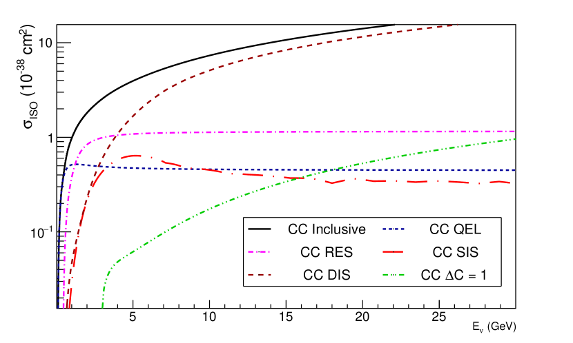
(a) $\nu_{\mu}$ CC on isoscalar targets.

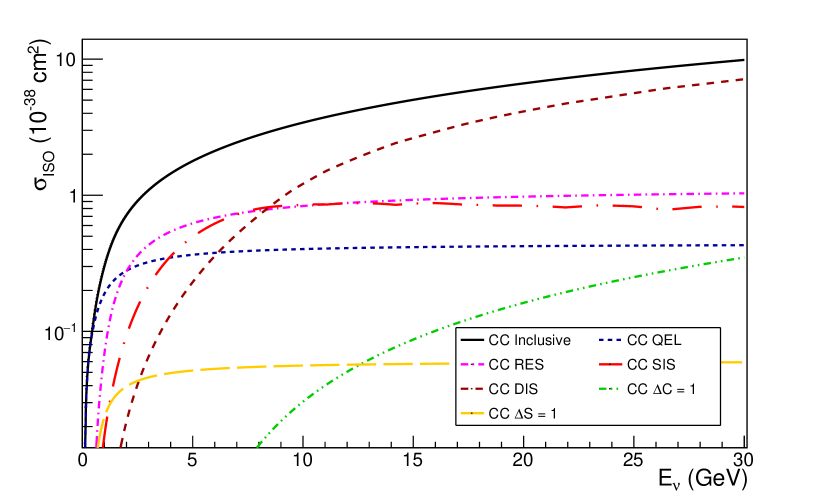
(b) $\bar{\nu}_{\mu}$ CC on isoscalar targets.

Figure 1: Summary of neutrino and anti-neutrino cross sections on isoscalar targets.

The term $d^{2}\sigma^{\text{SIS}}/dQ^{2}dW$ requires some elaboration. It represents the cross-section contribution from non-resonance shallow inelastic scattering in the resonance region. In GENIE, this cross section is computed with an empirical model where the Bodeck and Yang inclusive deep inelastic cross section is extrapolated into the resonance region and it is decomposed, via the GENIE AGKY [10] hadronization model, into the cross sections for different hadronic multiplicity channels. The extrapolation of the DIS model down to the inelastic threshold, $W<W_{\text{cut}}$, includes, on average, the effect of the resonances [11]. Notice that, even though the Bodeck and Yang model is capable of describing the inclusive cross section at inelastic threshold, we prefer to utilize an explicit resonance model. The contribution for hadronic multiplicities 2 and 3, that are responsible for producing many final states similar to those produced via resonance excitation, are tuned to remove double counting. This tuning is the main topic of this work.

The non-resonance shallow inelastic scattering cross section can be written as

$$\frac{d^{2}\sigma^{\text{SIS}}}{dQ^{2}dW}=\frac{d^{2}\tilde{\sigma}^{\text{DIS}}}{dQ^{2}dW} \cdot{\Theta}(W_{\text{cut}}-W)$$ (2)

$$\cdot{\sum\limits_{m}}f_{m}(Q^{2},W)$$

where $\tilde{\sigma}^{\text{DIS}}$ represents the extrapolated deep inelastic cross section into the resonance region, and $m$ refers to the multiplicity of the hadronic system. The factor $f_{m}$ relates the total calculated DIS cross section to the DIS contribution to this particular multiplicity channel. These factors are computed as

$$f_{m}(Q^{2},W)=R_{m}P^{\text{had}}_{m}(Q^{2},W)$$ (3)

where $R_{m}$ is an adjustable parameter and $P^{\text{had}}_{m}$ is the probability, taken from the GENIE hadronization model, that the DIS final state hadronic system multiplicity would be equal to $m$,

$$P^{\text{had}}_{m}(Q^{2},W)=\frac{1}{\langle m\rangle}\psi\left(\frac{m}{\langle m\rangle}\right)$$ (4)

The average hadronic multiplicity $\langle m\rangle$ is computed, for each value of hadronic invariant mass W, by

$$\langle m\rangle(Q^{2},W)=\alpha +\beta\ln\left(\frac{W^{2}}{\text{GeV}^{2}\text{/c}^{4}}\right)$$ (5)

$$+\beta^{\prime}\ln\left(\frac{Q^{2}}{\text{GeV}^{2}\text{/c}^{2}}\right)$$

and the function $\psi$ has the following asymptotic form

$$\psi(z)=\frac{2e^{-c}c^{cz+1}}{\Gamma(cz+1)}$$ (6)

In the above expressions, $\alpha$, $\beta$, $\beta^{\prime}$ and $c$ are adjustable parameters. In principle, $\alpha$, $\beta$, $\beta^{\prime}$ $c$ and $R_{m}$, are different for each initial state ($\nu+p$, $\nu+n$, $\bar{\nu}+p$, $\bar{\nu}+n$) and are different for charged current and neutral current interactions. A new tune of the neutrino-induced hadronization models in GENIE is currently in progress and, in future, it may be possible to perform a joint tuning of the GENIE cross section and hadronization modeling components for bare-nucleon targets. However, at this present work, the parameters $\alpha$, $\beta$, $\beta^{\prime}$ and $c$ were kept at the default values of the AGKY model in GENIE v3. For easy reference, the relevant values for the channels studied in this work are included in Tab. 1. No dependence on $Q^{2}$ has been observed in $\nu$ and $\bar{\nu}$ scattering data [12], hence $\beta^{\prime}=0$ for all channels.

For most inelastic processes simulated in neutrino-nucleus scattering by all current GENIE comprehensive model configurations, the total inelastic differential cross section for scattering off bare nucleons takes centre stage. In Fig. 1, the contribution to the $\nu_{\mu}$ CC and $\bar{\nu}_{\mu}$ CC inclusive cross sections on isoscalar targets in GENIE is shown for the different interaction processes. The CC RES and SIS/DIS CC cross-section contribution for different neutrino energies is shown in Fig. 2.

		Initial state
Parameter		$\nu_{\mu}p$	$\nu_{\mu}n$	$\bar{\nu}_{\mu}p$	$\bar{\nu}_{\mu}n$
$\alpha$		0.40	-0.20	0.02	0.80
$\beta$		1.42	1.42	1.28	0.95
$c$		7.93	5.22	5.22	7.93

Table 1: Relevant default GENIE v3 AGKY parameters for $\nu_{\mu}$ and $\bar{\nu}_{\mu}$ CC interactions on proton and neutron.

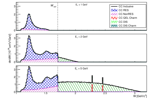
Figure 2: RES and SIS/DIS differential cross section as a function of the invariant mass for three different neutrino energies using a $1/E$-like flux. $W_{\text{cut}}$ divides the SIS and the DIS regions.

III Comprehensive model configurations in GENIE v3

GENIE has a large degree of configuration: for each process (RES, DIS, etc.) the system offers a number of alternative models to be used for event generation. In previous GENIE releases, only one model-process mapping was suggested by the out-of-the-box configuration, despite the availability of alternative models. Yet, there was no guidance on how to correctly use different configurations according to author and developers. In fact, processes are not universal and their definitions are generator dependent. Hence, it was easy to come up with inconsistencies between the model configuration for different processes that were supposed to be used together to get a correct comprehensive physics simulation.

This issue was addressed in GENIE v3 by introducing the concept of comprehensive model configuration (CMC) that is a consistent process-model association. Considering that GENIE already has about 20 different processes only for neutrinos, CMC definitions are quite complex objects and they need to be effectively named so that the community can use them unambiguously. For this purpose, the collaboration developed a specific naming convention, see Sec. III.1. Sec. III.2 describes the models used in CMCs relevant for neutrino interactions.

III.1 Comprehensive model configuration naming convention

A comprehensive model configuration is identified by at least 7-character string in the form:

Gdd_MMv

where

• G is a capital letter string of arbitrary length that identifies the authors of the tune (GENIE).

• dd is a number describing the year during which the model configuration was first developed.

• MM is a number (00, 01, 02, …) identifying a family of model configurations.

• v is a character (a, b, c, …) enumerating different members of the given family of model configurations.

Once a comprehensive model configuration is defined, a number of different tunes may be produced. These may be produced, for example, by a) incorporating different combinations of experimental data, b) considering variations in different combinations of our modelling elements (e.g. bare-nucleon cross sections, nuclear model and nuclear cross sections, neutrino-induced hadronization etc), c) considering different degrees of freedom (different parameterisations) for the variation of each model, or d) incorporating different parameter priors and/or different strategies for eliminating nuisance parameters. A tune is identified by the model configuration name, and additional information enumerating the parameters and datasets. This is at least 14-character string in the form:

Gdd_MMv_PP_xxx

where

• Gdd_MMv describes the model configuration (see above).

• PP is a number identifying the set of tuned parameters. This parameter set is defined uniquely only in the context of a particular model configuration.

• xxx is a number that identifies the dataset used for the model configuration tuning. This may include a unique set of weights associated with each component dataset.

III.2 CMCs available in GENIE v3

Several CMCs are available in GENIE v3, but they can be grouped together as their scopes are common. The first group of CMCs is historically motivated: it is based on the default configuration and simply provides updates for processes that were introduced later. The second family is an improvement of the first group, in terms of the resonance model. The third one was constructed aiming to deliver the most up to date theoretical nuclear matter simulations. Out of these main ideas, a number of CMCs can be constructed simply changing minor aspects like FSI or form factors. Here, we briefly summarise the modeling components used in each comprehensive model configuration available in GENIE v3.

III.2.1 G18_01a, G18_01b, G18_01c and G18_01d

These comprehensive models share an identical cross-section model construction, which is an adiabatic update of the historical default cross-section model of GENIE v2, now named as G00_00a CMC. For interactions on nucleons and nuclei, it relies on implementations of the following models: the Ahrens model [13] for NC elastic, the Llewellyn Smith model [14] for CC quasi-elastic, the Rein-Sehgal model [5] for NC and CC resonance production, the Rein-Sehgal model [15] for NC and CC coherent pion production, the Bodek-Yang model [9] for NC and CC deep inelastic scattering and non-resonance shallow inelastic scattering, the Kovalenko model [16] for quasi-elastic charm production, and the Aivazis-Olness-Tung slow rescaling model [17] for deep inelastic charm production. Nuclear cross sections are calculated within the framework of a relativistic Fermi gas model, following the approach of Bodek-Ritchie [18]. Multi-nucleon processes in neutrino scattering off nuclear targets can be optionally enabled and simulated via an empirical GENIE model [1]. In addition, in GENIE v3, the adiabatic upgrade of the historical comprehensive model includes the simulation of processes that, previously, were either optional or missing. This includes both diffractive pion production based on an implementation of the Rein model [19], and quasi-elastic $|\Delta S|=1$ hyperon ($\Lambda^{0}$, $\Sigma^{-}$, $\Sigma^{0}$) production based on the Pais model [20]. Single Kaon production, although optionally available for neutrinos in GENIE v3 [21], is not yet available for antineutrinos and inclusion in any published GENIE comprehensive configurations was postponed till an antineutrino implementation is available and the Kaon content of hadronic showers produced by GENIE has been retuned following the addition of the single-Kaon generator. Both G18_01a and G18_01b comprehensive models employ a revised resonance decay algorithm and an implementation of the AGKY [10] hadronization model that is unchanged with respect to that used at the latest releases of GENIE v2 series. Four comprehensive model variations are constructed by attaching different intranuclear hadron transport models to the same underlying cross section and hadronization models [22]. G18_01a uses an updated INTRANUKE hA effective intranuclear rescattering model which is unique to GENIE, G18_01b uses the new INTRANUKE hN model implementing a full intranuclear cascade including medium corrections, G18_01c uses an interface to the GEANT4 [23] Bertini intranuclear cascade [24] (version 4.10.2) and G18_01d uses an interface to the INCL++ (version 5.2.9.5) implementation of the Liège intranuclear model [25].

III.2.2 G18_02a, G18_02b, G18_02c and G18_02d

This is family of empirical models which is an evolved version of the G18_01[a-d] ones. The general construction of the cross-section model is similar to the one discussed above, with the exception that the implementations of the Rein-Sehgal models for CC and NC resonance neutrino-production, as well as for CC and NC coherent production of mesons, were replaced with updated models by Berger-Sehgal [8]. Similarly to G18_01[a-d], four comprehensive model variations are constructed by using alternative intranuclear hadron transport models on top of the same underlying cross section and hadronization models (a: INTRANUKE/hA, b: INTRANUKE/hN, c: GEANT4/Bertini, and d: INCL++).

III.2.3 G18_10a, G18_10b, G18_10c and G18_10d

This is a family of models derived from the improved empirical ones (G18_02[a-d]) described above, by substituting both the Llewellyn Smith CC quasi-elastic model [14] and GENIE’s empirical multinucleon model with implementations of the corresponding Valencia models by Nieves et al. [26]. This family of comprehensive models provides a firmer theoretical basis for the simulation of neutrino-nucleus scattering around the quasi-elastic peak. Within this family of models, the nuclear environment is modelled using a Local Fermi Gas, matching the inputs used for the published Valencia calculations. Again, four comprehensive model variations (a-d) are constructed by using alternative intranuclear hadron transport models, following the same naming convention introduced above. The implementation of the Valencia model in GENIE does not predict the kinematics of the outgoing hadrons and its description needs to be accompanied by one of the FSI models available in GENIE (a-d) [27].

III.2.4 G18_10i, G18_10j, G18_10k and G18_10l

These comprehensive models are derived from the G18_10[a-d] ones, by replacing the dipole axial form factor, used in the calculations of quasi-elastic cross sections, with the better-motivated z-expansion model [28], providing a richer set of degrees of freedom for parameterizing quasi-elastic model uncertainties. As in all previous families of models, four comprehensive model variations (i-l) are constructed by using alternative intranuclear hadron transport models, though the labelling is now different (i: INTRANUKE/hA, j: INTRANUKE/hN, k: GEANT4/Bertini, and l: INCL++).

III.3 Free nucleons and CMCs

Although a large number (16) of CMCs was summarised above, with respect to the cross sections for (anti)neutrino scattering off bare nucleons, there are only two different model constructions: The one used in a) G18_01[a-d], and the one used in b) G18_02[a-d], G18_10[a-d] and G18_10[i-l]. The main difference between these two model constructions resides mainly in the treatment of the lepton mass. Although some differences can be expected between G18_10[a-d] and G18_10[i-l], because of different choices in the modelling of the axial form factor for quasi-elastic scattering, they do not manifest themselves in the context of this particular analysis.

Several variations of the tuning procedure were run and evaluated for testing purposes, before converging to the procedure presented in this paper. Preliminary versions of this work were released in the GENIE v3 series (v3.0.0-v3.0.6) in a series of tunes carrying the 02_11a label. The final results presented in the paper will be made available in GENIE v3.2 in a series of 16 tunes, one for each of the 16 comprehensive model configurations summarised above, labelled as 02_11b. For example, the tune G18_10a_02_11b corresponds to the G18_10a comprehensive model with the parameters determined through the tuning procedure discussed in this paper (02_11b). The GENIE tune naming convention was discussed in an earlier section. A full list of GENIE tunes is maintained in http://tunes.genie-mc.org. The preliminary versions (02_11a) of the tunes will be kept in GENIE v3.2, but they will be phased out in subsequent minor releases.

IV Data and model uncertainties review

The data used in this analysis are old and a careful review of the past analysis procedure is required in order to combine all the data together in a global analysis. This section summarises the data details and how the models used in the fit behave in the same energy region.

IV.1 Datasets included in the fit and their systematics

In the current work, we consider Hydrogen and Deuterium data from the ANL 12FT, BNL 7FT, FNAL 15FT and BEBC bubble chamber experiments. The data represent integrated cross sections for different incoming neutrino energy bins for

• $\nu_{\mu}$ and $\bar{\nu}_{\mu}$ CC inclusive scattering [29, 30, 31, 32, 33, 34, 35, 36, 37, 38, 39, 40, 41, 42, 43, 44, 45, 46, 47, 48, 49, 50, 51, 52, 53, 54, 55, 56]

• $\nu_{\mu}$ and $\bar{\nu}_{\mu}$ CC quasi-elastic scattering [29, 39, 53, 57, 58, 59, 60, 61, 62, 63, 64, 65]

• $\nu_{\mu}$ and $\bar{\nu}_{\mu}$ CC single-pion production [66, 67, 68, 69, 70, 71, 72, 58, 73, 74]

  • $\nu_{\mu}+n\rightarrow\mu^{-}+n+\pi^{+}$

  • $\nu_{\mu}+p\rightarrow\mu^{-}+p+\pi^{+}$

  • $\nu_{\mu}+n\rightarrow\mu^{-}+p+\pi^{0}$

  • $\bar{\nu}_{\mu}+p\rightarrow\mu^{+}+p+\pi^{-}$

  • $\bar{\nu}_{\mu}+n\rightarrow\mu^{+}+n+\pi^{-}$

• $\nu_{\mu}$ CC two-pion production [75]

  • $\nu_{\mu}+p\rightarrow\mu^{-}+n+2\pi^{+}$

  • $\nu_{\mu}+p\rightarrow\mu^{-}+p+\pi^{+}+\pi^{0}$

  • $\nu_{\mu}+p\rightarrow\mu^{-}+n+\pi^{+}+\pi^{-}$

Not all of the available historical data has been used for the fit, as some datasets were superseded or reanalysed, as in the case of ANL 12FT and BNL 7FT, datasets. The latest analysis are used. A detailed summary of the datasets used in the fit is shown in Tab. 2 and in Fig. 3. Some of the datasets included in the tune consider Hydrogen-Neon mixtures. The nuclear effects of the neon in the target mixture are shown to be negligible [76].

Low energy bins have a higher contribution to the $\chi^{2}$ due to energy smearing and lack of unfolding in measurements. Hence, data points with $E_{\nu}<0.5$ GeV are removed from the fit. In total, the tune is performed with 169 data points from bubble chamber experiments. Different analysis methods were implemented in each experiment, such as cuts applied on the $W$ invariant mass, the outgoing muon momentum or the total longitudinal momentum of the final state. The associated GENIE prediction has been corrected by applying the same cuts to the generated events. Moreover, datasets from the same experiments are not independent as they share the same neutrino flux, detector, analysis methodology, etc. Although it is clear that some correlated uncertainties exist, the data releases do not contain any information about the correlation between them. In the GENIE database, we added a systematic error to the datasets of 15%. The methodology used to include them in the fit is detailed in Sec. V.3. Other free nucleon data on heavier targets are available but used only for comparison with the GENIE prediction. No correction for nuclear effects is considered for deuterium targets.

Experiment	$\mathbf{N_{p}}$	Energy [GeV]	Target	Cuts	Ref.
$\nu_{\mu}+N\rightarrow\mu^{-}X$
BNL 7FT	13	0.6-10	2H		[44]
BEBC	3	10-50	H-10Ne		[42]
FNAL	6	10-110	2H		[74]
	5	100-110	H-10Ne		[47]
$\bar{\nu}_{\mu}+N\rightarrow\mu^{+}X$
BEBC	3	11-110	1H-10Ne		[30]
	1	10-50	1H-10Ne		[42]
	6	30-110	1H-10Ne		[31]
	1	10-110	1H-10Ne		[43]
BNL 7FT	1	1-4	1H		[53]
FNAL	5	10-110	2H$-^{10}$Ne		[49]
	7	10-80	2H$-^{10}$Ne		[54]
$\nu_{\mu}n\rightarrow\mu^{-}n\pi^{+}$
ANL 12FT	5	0.3-2	1H and 2H		[67]
ANL 12FT,ReAna	7	0.3-3	2H		[68]
BNL 7FT,ReAna	11	0.1-4	2H		[68]
$\nu_{\mu}p\rightarrow\mu^{-}p\pi^{+}$
ANL 12FT,ReAna	8	0-1.6	2H		[68]
BNL 7FT,ReAna	7	0-7	2H		[68]
BEBC	7	1-30	1H	$W<1.4$ GeV	[70]
	6	5-100	2H	$W<2$ GeV	[58]
	5	10-80	1H	$W<2$ GeV	[72]
FNAL	3	10-30	1H	$W<1.4$ GeV	[77]
$\nu_{\mu}n\rightarrow\mu^{-}p\pi^{0}$
ANL 12FT	5	0.2-2	1H and 2H		[67]
ANL 12FT,ReAna	7	0.2-2	2H		[68]
BNL 7FT,ReAna	10	0.4-3	2H		[68]
$\nu_{\mu}p\rightarrow\mu^{-}n\pi^{+}\pi^{+}$
ANL 12FT	5	1-6	2H		[75]
$\nu_{\mu}p\rightarrow\mu^{-}p\pi^{+}\pi^{0}$
ANL 12FT	5	1-6	2H		[75]
$\nu_{\mu}n\rightarrow\mu^{-}p\pi^{+}\pi^{-}$
ANL 12FT	5	8-6	2H		[75]
BNL 7FT	10	0-20	2H		[35]
$\bar{\nu}_{\mu}p\rightarrow\mu^{+}p\pi^{-}$
FNAL	1	5-70	1H	$W<1.9$ GeV	[73]
$\nu_{\mu}+n\rightarrow\mu^{-}+p$
ANL 12FT	7	0-2	2H		[57]
	8	0-2	1H and 2H		[29]
BNL 7FT	4	0.2-2	2H		[62]
BEBC	5	20-40	2H		[58]
FNAL	2	0-50	2H		[59]

Table 2: A summary of cross-section data used in this work. The number of data points released by each analysis ($N_{p}$), the neutrino energy range covered $E_{\nu}$, the type of target and the cuts applied in the analysis procedure are specified in the table.

(a) $\nu_{\mu}$ CC cross section.

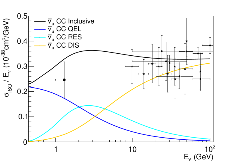
(b) $\bar{\nu}_{\mu}$ CC cross section.

Figure 3: Charged current cross section on isoscalar targets as a function of the incoming neutrino energy. Breakdown of quasi-elastic, one and two pion production and deep inelastic processes is shown. The predictions are computed using the G18_02a_00_000 configuration. The data on hydrogen and deuterium targets from Tab. 2 is shown if available from ANL 12FT ($\bigtriangleup$), BNL 7FT ($\bullet$), BEBC ($\diamond$) and FNAL ($\star$).

IV.2 Model uncertainties

The SIS cross section is tuned within the CMCs using either the Rein-Sehgal or Berger-Sehgal resonance models, see Sec. III.2. The tuning main goal is the best value estimation for nine of the parameters that drive the GENIE predictions in the SIS region. These parameters are the $W_{\text{cut}}$ as defined in Eq. 1, the four $R_{m}$ coefficients for CC interactions on neutron/proton with $m=2,3$ from of the SIS region (Eq. 3), the axial masses used in the dipole form factors for RES and QE interactions, and 2 global scaling factors for the RES cross section and the DIS cross section. For clarity, we will refer to $R_{m}$ parameters with the number of pions in the final state, namely $R_{\nu p}^{\text{CC}1\pi}$,$R_{\nu p}^{\text{CC}2\pi}$, $R_{\nu n}^{\text{CC}1\pi}$ and $R_{\nu n}^{\text{CC}2\pi}$. Tab. 3 summarises the parameter pre-fit values and the allowed ranges. Previous fits to data are taken into account for the determination of the ranges [78, 79].

Parameter	GENIE parameter name	Default value	Min value	Max value	Prior
$W_{\text{cut}}$ (GeV/c2)	Wcut	1.7	1.5	2.3
$M_{A}^{\text{QE}}$ (GeV/c2)	QEL-Ma	0.999	0.75	1.10	$1.014\pm 0.014$ [80]
$M_{A}^{\text{RES}}$ (GeV/c2)	RES-Ma	1.12	0.8	1.3	$1.12\pm 0.03$ [78]
$R_{\nu p}^{\text{CC}1\pi}$	DIS-HMultWgt-vp-CC-m2	0.10	0.0	0.4
$R_{\nu p}^{\text{CC}2\pi}$	DIS-HMultWgt-vp-CC-m3	1.00	0.0	2.0
$R_{\nu n}^{\text{CC}1\pi}$	DIS-HMultWgt-vn-CC-m2	0.30	0.0	0.35
$R_{\nu n}^{\text{CC}2\pi}$	DIS-HMultWgt-vn-CC-m3	1.00	0.8	3.0
$S_{\text{RES}}$	RES-CC-XSecScale	1.0	0.6	1.2
$S_{\text{DIS}}$	DIS-CC-XSecScale	1.032	0.9	1.15	$1\pm 0.05$

Table 3: Parameters of interest of the tunes and their statistical properties as used in the fitting procedures. The Default values correspond to the nominal values from GENIE v2 [1].

Each of the parameters have a different sensitivity to each dataset, as different scattering mechanisms are involved. The response of each parameter in the inclusive and exclusive cross sections is studied by varying each of them independently within the studied range. In Fig. 4, each parameter response is shown for inclusive and exclusive cross sections. When more than one parameter in the plot is impacting the same cross section, i.e. CC inclusive, the variations are added in quadrature.

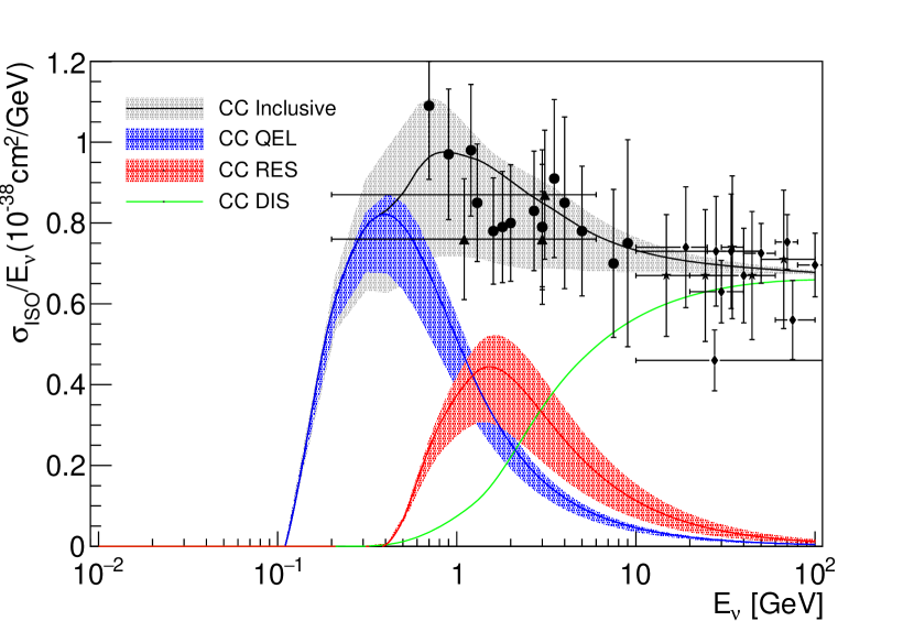
(a) $M_{A}^{\text{RES}}$ and $M_{A}^{\text{QE}}$ impact.

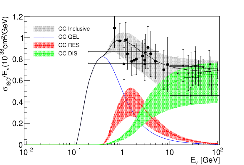
(b) $S_{\text{RES}}$ and $S_{\text{DIS}}$ impact.

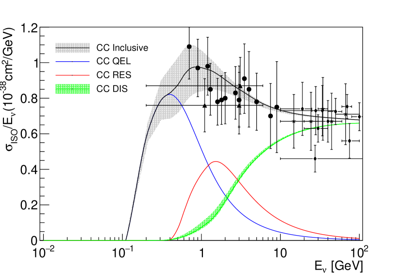
(c) $R_{\nu p}^{\text{CC}1\pi}$, $R_{\nu p}^{\text{CC}2\pi}$, $R_{\nu n}^{\text{CC}1\pi}$ and $R_{\nu n}^{\text{CC}2\pi}$ impact.

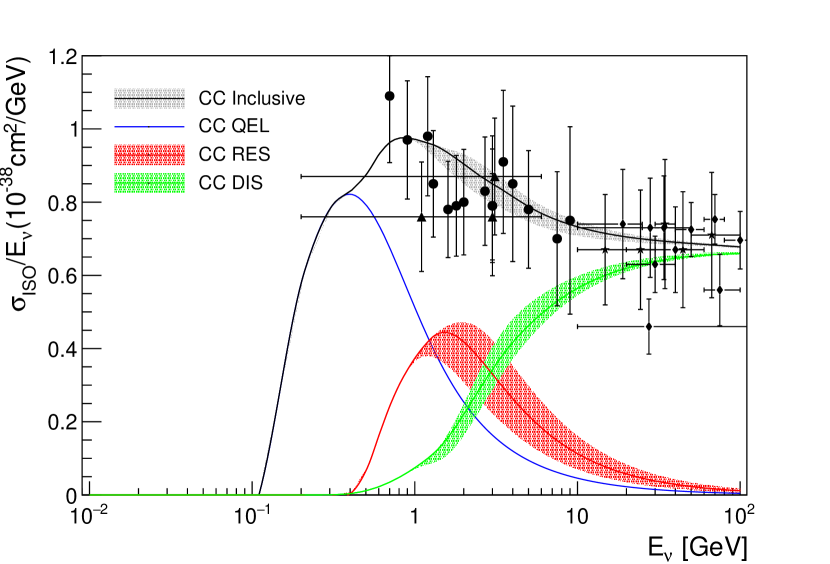
(d) $W_{\text{cut}}$ impact.

Figure 4: $\nu_{\mu}$ CC Inclusive G18_02a prediction against hydrogen and deuterium data. Each parameter response is characterized within the tuned region, specified in Tab. 3. Data corresponding to hydrogen and deuterium targets from ANL 12FT ($\bigtriangleup$), BNL 7FT ($\bullet$), BEBC ($\diamond$) and FNAL 15FT ($\star$).

At the Monte Carlo level, where no correlation between the parameters is considered, the impact of each of the parameters in the cross section can be classified as influencing a variation on

1. The CC Quasi-Elastic cross section

2. The CC RES cross section

3. The CC DIS cross section

For instance, $M_{A}^{\text{QE}}$ will only affect the quasi-elastic cross section prediction, as summarized in Fig.  4(a). Notice though that, at the tune level, this will no longer hold as the introduction of flux nuisance parameters correlates exclusive channels. Hence, this will introduce a correlation between $M_{A}^{\text{QE}}$ and the SIS parameters.

The description of the CC RES cross section will be affected by the RES axial mass $M_{A}^{\text{RES}}$ (Fig. 4(a)), the resonant scaling parameter $S_{\text{RES}}$ (Fig. 4(b)), and $W_{\text{cut}}$ (Fig. 4(d)). The default G18_01a and G18_02a configurations overestimate one-pion production processes, and would favor a reduction in the CC RES cross section. Variations of $M_{A}^{\text{RES}}$ have a huge impact on both exclusive and inclusive CC cross sections in the few-GeV region. However, as it is explained in Sec. V.3, this parameter should agree with the world average extracted from fits to the axial form factor [78] and a deviation from this result is disfavoured by previous fits to data. Consequently, a reduction of $S_{\text{RES}}$ is expected to improve the agreement with one-pion production data. On the other hand, $W_{\text{cut}}$ will play an important role as it determines the number of resonances included in the CC RES calculation. The current default, $W_{\text{cut}}=1.7$ GeV/$c^{2}$, discards the resonances contributing at $W>W_{\text{cut}}$. Therefore, an increase on $W_{\text{cut}}$ will incorporate new resonances in the calculation that were not taken into account in previous tunes. This increase is favoured by two-pion production data, as heavier resonances producing more than one pion are incorporated.

The SIS region is treated by combining two cross-section models, one for DIS and one for RES interactions. Thus, in that region, many parameters have a visible effect on the predictions as can be seen in Fig. 4: regardless of the parameter considered in the plot, there is always a visible error band in the few-GeV region. This is a clear hint for the presence of degeneracy that must be faced by our global tunes. An example of this is given by the $R_{n}$ and the $S_{DIS}$ parameters, which act as scaling factors for the DIS contribution at $W<W{cut}$. As mentioned above, a desired result of the tune is to reduce the one-pion prediction and increase the two pion production. This can be accomplished via alterations of either the $R_{n}$ and/or the $S_{DIS}$ parameters.

V Bare-nucleon cross-section tuning procedure

This section describes the core ideas behind the paper. Most of these are not specific for this work: they are general concepts developed within the GENIE tuning system and can therefore apply to future tune releases.

V.1 Likelihood construction

The GENIE integrated cross-section prediction is denoted with $\sigma^{i}_{\text{th}}(E_{k}|\bm{\theta})$, where $E_{k}$ is the neutrino energy, $\bm{\theta}$ is a vector of the adjustable physics parameters introduced in Sec. IV.2, and $i$ is any of the 10 reaction processes considered in the work presented in Tab. 2. Using $\sigma^{i}_{\text{th}}(E|\bm{\theta})$, we produce the corresponding prediction for the $k$-th energy bin of the $j$-th dataset for the $i$-th reaction type,

$$\sigma^{ij}_{\text{th}}(E_{k}|\bm{\theta})=\varepsilon^{ij}(E_{k},\bm{\theta})\,\sigma^{i}_{\text{th}}(E_{k}|\bm{\theta})$$ (7)

where $\varepsilon^{ij}(E_{k},\bm{\theta})$ are dataset-dependent efficiencies expressing the fraction of events from the $i$-th process that survive the kinematical cuts imposed by the experiment, see Tab. 2. The statistical error due to the MC sample size is also evaluated and this is denoted $\delta\sigma^{ij}\left(E_{k}|\bm{\theta}\right)$.

Performing a multi-parameter brute-force scan and tune using $\sigma^{ij}_{\text{th}}(E_{k}|\bm{\theta})$ is computationally inefficient. As was highlighted in the introduction, the GENIE global analysis framework relies on Professor [2] to reduce the computational complexity of brute-force scans while allowing for massive parallelisation. Using the values of $\sigma^{ij}_{\text{th}}(E_{k}|\bm{\theta})$ computed for a number ($N_{R}$) of randomised P-dimensional vectors $\bm{\theta}$, produced within the P-dimensional hyper-cube defined by the parameter ranges given in Tab. 3, we use Professor to generate a parameterisation of $\sigma^{ij}_{\text{th}}(E_{k}|\bm{\theta})$ and $\delta\sigma^{ij}(E_{k}|\bm{\theta})$ that will be denoted with $\widetilde{\sigma}^{ij}_{\text{th}}(E_{k}|\bm{\theta})$ and $\delta\widetilde{\sigma}^{ij}(E_{k}|\bm{\theta})$ respectively. As discussed in [2], the parameterisation is a generic polynomial of order $M$ in the P-dimensional space, whose analytical form is

$$\widetilde{\sigma}^{ij}_{\text{th}}(E_{k}|\bm{\theta}) = \alpha_{0}^{ijk}+\sum_{n=1}^{P}\beta_{n}^{ijk}\theta_{n}+\sum_{n\leq m}\gamma_{nm}^{ijk}\theta_{n}\theta_{m}$$ (8)

$$+ \ldots+\sum_{n_{1}\leq\ldots\leq n_{M}}\!\!\!\!\!\!\xi^{ijk}_{n_{1}\ldots n_{M}}\prod_{\ell=1}^{M}\theta_{n_{\ell}}$$

where $\theta_{n}$ is the coordinate of the $n$-th parameter. The polynomial order $M$ is set by the user. The coefficients $\alpha_{0}^{ijk}$, $\beta_{n}^{ijk},\gamma_{(nm)}^{ijk},\ldots,\xi^{ijk}_{(n_{1}\ldots n_{M})}$ are determined by Professor fitting the parameterisation against the computed $\sigma^{ij}_{\text{th}}(E_{k}|\bm{\theta})$. In the analysis presented here, a 4${}^{\text{th}}$ order polynomial was used for the G18_01a comprehensive model configuration while a 5${}^{\text{th}}$ order polynomial was used for G18_02a. Particularly, $N_{R}=1500$ for G18_01a and $N_{R}=2183$ for G18_02a. The accuracy of the parameterisation is demonstrated in the residual distributions shown in Fig. 5. The parameterisation $\widetilde{\sigma}^{ij}_{\text{th}}(E_{k}|\bm{\theta})$ is used instead of the exact predictions in order to to estimate the best-fit parameters by minimising the $\chi^{2}$.

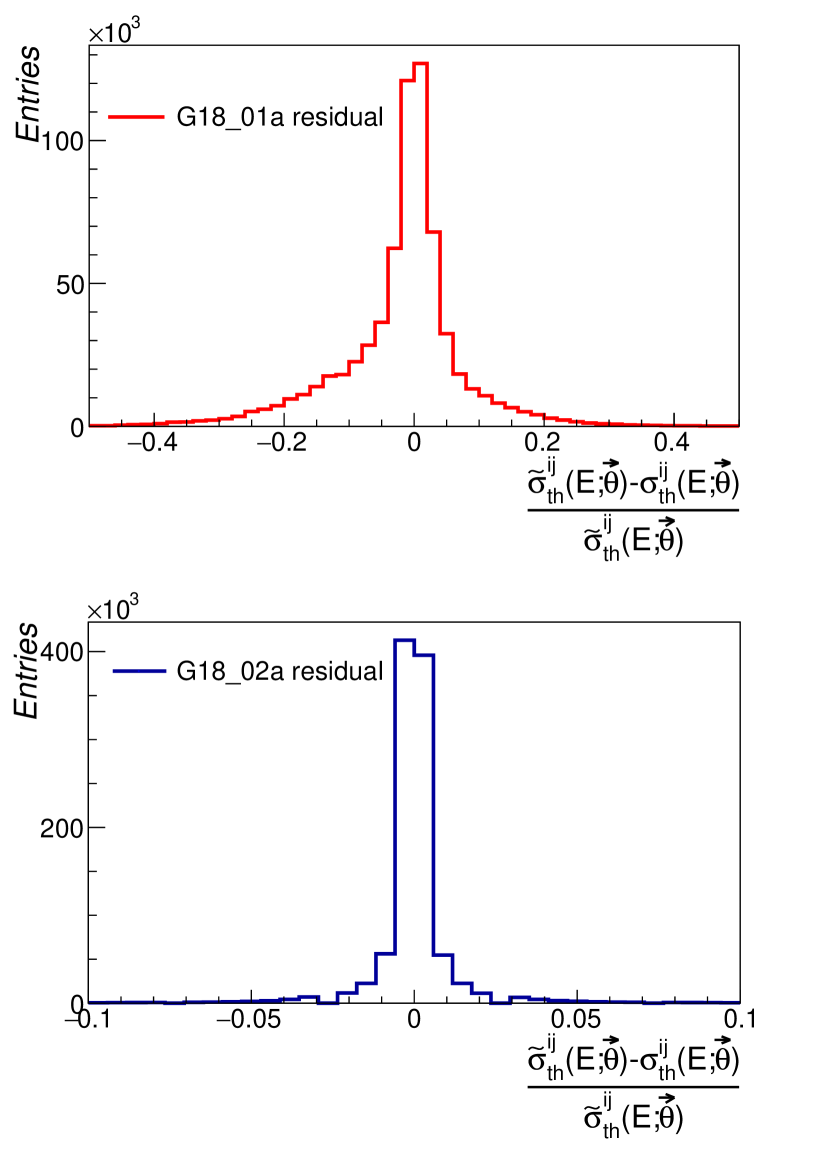
Figure 5: Fractional difference between true Monte Carlo predictions calculated with a given $\vec{\theta}$ set vs the Professor parameterisation for both tunes. The G18_02a(b) parameterisation is improved as the number of scan points used and polynomial order $M$ are higher.

V.2 Treatment of systematic uncertainties

A number of nuisance parameters, each with a corresponding prior, can also be used to tackle the problem of correlated datasets. As seen in Sec. IV.1, there are different datasets coming from the same experiments (ANL 12FT, BNL 7FT, BEBC, and FNAL 15FT). Each of these experiments share the same flux (from either a neutrino or an antineutrino beam), analysis procedure, etc. Therefore, there is a correlation between the datasets, even though it has not been quantified in the data releases. A possible approach is to add nuisance parameters that can connect datasets from experiments that used the same neutrino beam. As the main systematic uncertainty comes from the fluxes, the nuisance parameters will act as scaling factors for our predictions ($\widetilde{\sigma}^{ij}_{\text{th}}(E_{k}|\bm{\theta})$) and are same for datasets sharing the same flux.

Some of the ANL 12FT and BNL 7FT data were already corrected for the flux normalization [68]. Due to this correction, the associated systematic error is smaller and, accordingly, a more restricted nuisance parameter is applied to the re-analysed datasets. These restricted parameters take into account other common systematics like reconstruction procedures, so they multiply all the predictions related to the same experiment. At the end of this procedure, each prediction can be scaled by up to 2 nuisance parameters, one for the flux and one for the remaining systematics. Thus, a total of 9 independent nuisance parameters are used to account for the correlation between datasets. They are all the available combinations of experiment and neutrino flux exposure ($\nu_{\mu}$ and $\bar{\nu}_{\mu}$) plus the restricted parameters for re-analysed data:

$$\bm{f}= \Big{(}f^{\text{AN}L}(\nu_{\mu}),f^{\text{ANL}}_{\text{Re}}(\nu_{\mu}),f^{\text{BNL}}(\nu_{\mu}),$$

$$f^{\text{BNL}}_{\text{Re}}(\nu_{\mu}),f^{\text{BNL}}(\bar{\nu}_{\mu}),f^{\text{BEBC}}(\nu_{\mu}),$$

$$f^{\text{BEBC}}(\bar{\nu}_{\mu}),f^{\text{FNAL}}(\nu_{\mu}),f^{\text{FNAL}}(\bar{\nu}_{\mu})\Big{)}$$

Quasi-elastic data for hydrogen and deuterium targets is included in the tune in order to constrain the nuisance parameters. Even though quasi-elastic data is not directly constraining the SIS parameters, it plays an important role to further constrain the fluxes of each experiment, as it is known at the 15 % level.

The main advantage of this method is the unbiased choice of the nuisance parameters, as their values will be determined by the minimization of the likelihood function. For the calculation of best-fit points and the calculation of intervals, these nuisance parameters are profiled (on every instance of our fit, they are eliminated by substituting them with the value that minimises $\chi^{2}$).

V.3 Discussion of priors

The likelihood is corrected using priors on parameters of interest ($\bm{\theta}$) and nuisance parameters ($\bm{f}$). Priors allow us to incorporate in this analysis the appropriate pre-fit uncertainties and correlations for the parameters of interest. Only Gaussian priors are considered at present.

The priors applied to each nuisance parameter $f_{j}$ have a peak at 1 and different standard deviations $\delta f_{j}$. In general the total scaling factor applied to non-re-analysed datasets are constrained by a conservative 15 % $\delta f$ Gaussian prior, except for those nuisance parameters that act on the same experiment. Thus, the BEBC and FNAL 15FT experiments have only one associated scaling factor $\delta f^{\text{BEBC}}=\delta f^{\text{FNAL}}=0.15$ for both neutrino and anti-neutrino fluxes; the same is true for $f^{\text{BNL}}(\bar{\nu}_{\mu})$. Up to two nuisance parameters can be applied to ANL 12FT and BNL 7FT data (i.e. $f^{ANL}(\nu_{\mu})$ and $f^{ANL}_{Re}(\nu_{\mu})$). The ANL 12FT and BNL 7FT restricted nuisance parameters, $f^{\text{ANL}}_{\text{Re}}(\nu)$ and $f^{\text{BNL}}_{\text{Re}}(\nu)$, have $\delta f=5\%$. $\delta f^{\text{ANL}}$ and $\delta f^{\text{BNL}}$ are such that ANL 12FT and BNL 7FT non-re-analysed datasets data are constrained by an overall $15\%$ Gaussian. The full summary of the nuisance parameters is in Tab. 4.

Parameter	Prior
$f^{\text{ANL}}(\nu_{\mu})$	$1\pm 0.14$
$f^{\text{ANL}}_{\text{Re}}(\nu_{\mu})$	$1\pm 0.05$
$f^{\text{BNL}}(\nu_{\mu})$	$1\pm 0.14$
$f^{\text{BNL}}_{\text{Re}}(\nu_{\mu})$	$1\pm 0.05$
$f^{\text{BNL}}(\bar{\nu}_{\mu})$	$1\pm 0.15$
$f^{\text{BEBC}}(\nu_{\mu})$	$1\pm 0.15$
$f^{\text{BEBC}}(\bar{\nu}_{\mu})$	$1\pm 0.15$
$f^{\text{FNAL}}(\nu_{\mu})$	$1\pm 0.15$
$f^{\text{FNAL}}(\bar{\nu}_{\mu})$	$1\pm 0.15$

Table 4: Nuisance parameters, $f^{j}$, per experiment (ANL 12FT, BNL 7FT, BEBC or FNAL 15FT) and neutrino beam ($\nu_{\mu}$ or $\bar{\nu}_{\mu}$). Priors consider the systematic uncertainty applied to each dataset as $\delta f_{j}$, where $j$ is one of the datasets under study. The allowed range is $[0,2]$ for nuisance parameters considered in the tune.

Priors are applied to the parameters of interest to penalize disagreement with well-established parameter values. For instance, the description of neutrino CC quasi-elastic cross sections and single-pion production through baryon resonances is strongly determined by the shape of the weak axial and vector transition form factors. For the G18_01a(/b/c/d) and G18_02a(/b/c/d) CMCs, the axial form factors are described using the dipole parameterisation which is a function of the invariant transferred momentum ($Q^{2})$:

$$F_{A}(Q^{2})=F_{A}(0)\left(1-\frac{Q^{2}}{M_{A}^{2}}\right)^{-2}$$ (9)

with $F_{A}(0)=g_{A}=-1.2695\pm 0.002$ [83]. The axial mass, $M_{A}$, is extracted from data. There are different masses for every interaction type: $M_{A}^{\text{QEL}}$ and $M_{A}^{\text{RES}}$. Both of these are evaluated from neutrino data on deuterium targets. The latest world average values for the axial masses are:

$$M_{A}^{\text{QE}}= \ 1.014\pm 0.014\enskip\text{GeV}/c^{2}$$ [80]

$$M_{A}^{\text{RES}}= \ 1.12\pm 0.03\enskip\text{GeV}/c^{2}$$ [78]

The extraction of these parameters requires neutrino differential cross sections as a function of $Q^{2}$ that are not used in this analysis. Our goal is not the extraction of the axial masses but the better estimation of the cross section at the SIS region. For this reason, these values are used as priors in our global fits.

Another parameter of interest which is strongly constrained by data is the $S_{\text{DIS}}$ parameter. This parameter dominates the cross-section behaviour at high neutrino energies. Most of the data in that energy range comes from neutrino interactions with heavy nuclear targets and are therefore not included in the fit. A Gaussian prior is considered to ensure that agreement with these data are preserved by our tuning procedure. This would not be the case otherwise as the SIS region data would prefer much higher cross-section values for the DIS contribution. The prior on $S_{\text{DIS}}$ provides a good solution for this problem because the degeneracy between DIS and non-resonant background parameters gives us multiple ways to accommodate good agreement between data and GENIE predictions in the SIS region. In other words, the introduction of the $S_{\text{DIS}}$ prior breaks the degeneracy without adding more datasets to the fit.

V.4 Final form of the $\chi^{2}$

Including all of the contributions from the previous sections and defining $\sigma^{ijk}_{d}$ ($\delta\sigma^{ijk}_{\text{stat}}$) as the data central value (statistical error) corresponding to the $\widetilde{\sigma}^{ij}_{\text{th}}(E_{k}|\bm{\theta})$ prediction, the complete form of our $\chi^{2}$ distribution becomes:

$$\chi^{2}(\bm{\theta},\bm{f})= \sum_{i,j,k}w^{ijk}\frac{(\phi_{j}(\bm{f})\widetilde{\sigma}^{ij}_{\text{th}}(E_{k}|\bm{\theta})-\sigma^{ijk}_{d})^{2}}{(\delta\sigma^{ijk}_{\text{stat}})^{2}}$$

$$+(\bm{\theta}-\bm{\theta}_{0})^{T}\Sigma^{-1}_{\theta}(\bm{\theta}-\bm{\theta}_{0})$$

$$+\sum_{j}\frac{(f_{j}-1)^{2}}{(\delta f_{j})^{2}}$$

where $\phi_{j}(\bm{f})$ is the product of the nuisance scaling factors that are relevant for $j$-th dataset as described in Sec. V.2. $\bm{\theta}_{0}$ and $\Sigma_{\theta}$ are the central values and the covariance matrix of the priors for the parameters of interest, respectively. Equation V.4 represents the full capability of our tuning machinery. However, the priors we applied for the present work were uncorrelated and so only the diagonal entries of $\Sigma_{\theta}$ were used. The details on the priors applied in this analysis are described in Sec. V.3.

The contribution of each point to the likelihood can be (de-)emphasized using weights $w^{ijk}$ to set the relative importance of different datasets (or of individual data points within a dataset). Such weighting schemes have been used extensively in general-purpose event generator tunes for the LHC (for an example, see [85]). In this particular analysis, the weights are used to include or exclude datasets only ($w^{ijk}\in\{0,1\}$).

VI Tuning results

In order to properly understand the global tune, the tensions between datasets must be discussed. These tensions are studied by performing fits using a specific dataset to evaluate the impact of the partially-fitted predictions on the rest of the datasets included in the global tune.

VI.1 Partial fits

Two main subsets were identified in the global dataset in order to study tensions: inclusive and exclusive datasets. The fits consider the G18_02a CMC as the base configuration and include nuisance parameters to take into account the correlation between datasets from the same experiment, see Sec. V for more details. No priors on $M_{A}^{\text{RES}}$ and $M_{A}^{\text{QE}}$ are applied as we are interested to see the impact of each subset on the prediction. The fit to inclusive data only is not sensitive to the scaling multiplicity parameters for the non-resonant background, therefore those parameters are fixed to their default values during the fit.

Parameter	Inclusive	Exclusive
$W_{\text{cut}}(\text{GeV})$	1.52	2.00
$M_{A}^{\text{QE}}(\text{GeV}/\text{c}^{2})$	$0.98\pm 0.01$	$1.003\pm 0.008$
$M_{A}^{\text{RES}}(\text{GeV}/\text{c}^{2})$	$1.15\pm 0.02$	$0.88\pm 0.02$
$R_{\nu p}^{\text{CC}1\pi}$	(0.10)	$0.30\pm 0.02$
$R_{\nu p}^{\text{CC}2\pi}$	(1.00)	$1.28\pm 0.06$
$R_{\nu n}^{\text{CC}1\pi}$	(0.30)	$0.294\pm 0.002$
$R_{\nu n}^{\text{CC}2\pi}$	(1.00)	$3.19\pm 0.09$
$S_{\text{RES}}$	$0.87\pm 0.03$	$0.88\pm 0.02$
$S_{\text{DIS}}$	$1.027\pm 0.005$	$1.026\pm 0.007$

Table 5: Parameter best-fit results for partial fits to inclusive and exclusive data using the G18_02a CMC as base configuration. Values within parentheses are kept fixed during the fit: they are the historical default values.

Partial fit results for inclusive and exclusive data are presented in Tab. 5. The tune against inclusive data only achieves much better agreement with inclusive data than the previous GENIE G18_02a default, see Fig.  6. This difference between the old and new inclusive tune is due to 1) the inclusion of only hydrogen and deuterium datasets and 2) the effect of the nuisance parameters. Particularly, without exclusive data, a small reduction of the resonant cross section is already observed in the CC RES region. The result for $M_{A}^{\text{RES}}$ is consistent with previous results without the addition of priors [78]. $W_{\text{cut}}$ is pulled to the lower edge of the parameter range: the parameter uncertainty could not be estimated as the $\chi^{2}$ minimum was found on the contour.

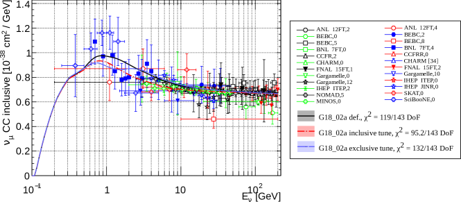
Figure 6: Comparison of $\nu_{\mu}$ CC Inclusive cross section against bubble chamber data. The default GENIE configuration corresponds to the G18_02a CMC. The inclusive tune is performed using the filled datapoints only. The predictions are computed with GENIE version 3.2 using the parameters specified in Tab. 5. The $\chi^{2}$ values are calculated against all inclusive data available from bubble chamber experiments.

As expected, the fit to exclusive data only is able to correctly describe exclusive datasets for one and two pion production. The low cross-section data for one pion production forces all the relevant parameters to decrease with respect to the default values see Fig. 7(a). At the same time, two pion production data forces $R_{\nu p}^{\text{CC}2\pi}$, $R_{\nu n}^{\text{CC}2\pi}$ and $W_{\text{cut}}$ to increase in order to match two pion production data, see Fig. 7(b). The agreement with $\nu_{\mu}$ CC inclusive data is worse, see Fig. 6, but the compatibility is still acceptable given the large uncertainties on the data in that region. On the other hand, the partial fit does not obtain a good prediction for $M_{A}^{\text{RES}}$. $W_{\text{cut}}$ is fixed to its maximum value of 2 GeV to avoid nonphysical regions.

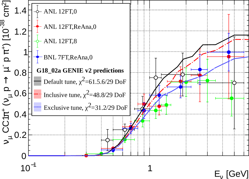
(a) Comparison against $\nu_{\mu}CC1\pi^{+}$ data.

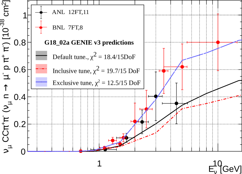
(b) Comparison against $\nu_{\mu}CC\pi^{+}\pi^{-}$ data.

Figure 7: Comparison of $\nu_{\mu}$ CC exclusive channels against bubble chamber data. The default GENIE configuration corresponds to the G18_02a CMC. The exclusive tune is sensitive to the exclusive datasets only, see Tab. 2. The predictions are computed with GENIE version 3.2 using the parameters specified in Tab. 5. The $\chi^{2}$ values are calculated against all exclusive data shown in each plot.

The exclusive fit clearly shows a preference for a larger total cross section in the neutrino energy region between 1 and 10 GeV due to the high value of $R_{\nu p}^{\text{CC}2\pi}$ and $R_{\nu n}^{\text{CC}2\pi}$. This is a tension between exclusive and inclusive datasets as the inclusive prefer a lower value in that $E_{\nu}$ region. Since inclusive data constitute about $40\%$ of all the data points, the inclusion of priors for the axial masses and $S_{\text{DIS}}$ becomes crucial to overcome the tension [87].

VI.2 Global fit

The analysis procedure outlined in previous sections was applied to the comprehensive model configurations listed in Sec. III. The best-fit parameter values obtained from the GENIE analysis for each alternative CMC are shown in Tab. 6 and Tab. 7. The GENIE v3 cross-section curves that correspond to the two sets of tuned parameters are shown in Figs. 8, 9, 10, 12 and 11. For reference, we also show the cross-section predictions made by the default G18_02a CMC that is available in the last public release of the GENIE v3 series (3.2).

Parameter	G18_01a(/b)	G18_02a(/b)
$W_{\text{cut}}$	$1.94$	$1.81$
$M_{A}^{\text{QE}}$	$1.00\pm 0.01$	$1.00\pm 0.013$
$M_{A}^{\text{RES}}$	$1.09\pm 0.02$	$1.09\pm 0.014$
$R_{\nu p}^{\text{CC}1\pi}$	$0.06\pm 0.03$	$0.008$
$R_{\nu p}^{\text{CC}2\pi}$	$1.1\pm 0.2$	$0.94\pm 0.075$
$R_{\nu n}^{\text{CC}1\pi}$	$0.14\pm 0.03$	$0.03\pm 0.010$
$R_{\nu n}^{\text{CC}2\pi}$	$2.8\pm 0.4$	$2.3\pm 0.12$
$S_{\text{RES}}$	$0.89\pm 0.04$	$0.84\pm 0.028$
$S_{\text{DIS}}$	$1.03\pm 0.02$	$1.06\pm 0.01$
$\chi^{2}$/157 DoF	$1.84$	$1.64$

Table 6: Best-fit parameter values and parameter ranges obtained by requiring that ${\Delta\chi^{2}_{\text{profiled}}<\Delta\chi^{2}_{\text{critical}}=1}$. Results are shown for all alternative CMCs considered in this analysis. The best-fit values obtained for the G18_02a(/b) CMC can be used for the G18_10a(/b) as the same bare-nucleon underlying models are used. Moreover, for the G18_10i(/j) CMCs, the best-fit values from the G18_02a(/b) tune can also be used, except for $M_{A}^{\text{QE}}$, as the quasi-elastic axial form factor is parametrised with the z-expansion model instead of a dipole and the corresponding z-expansion parameters are kept to the default values.

Parameter	G18_01a(/b)	G18_02a(/b)
$f^{\text{ANL}}(\nu_{\mu})$	$0.98\pm 0.05$	$0.89\pm 0.05$
$f^{\text{ANL}}_{\text{Re}}(\nu_{\mu})$	$1.12\pm 0.05$	$1.2\pm 0.05$
$f^{\text{BNL}}(\nu_{\mu})$	$1.01\pm 0.04$	$1.06\pm 0.04$
$f^{\text{BNL}}_{\text{Re}}(\nu_{\mu})$	$1.08\pm 0.05$	$1.03\pm 0.04$
$f^{\text{BNL}}(\bar{\nu}_{\mu})$	$1.00\pm 0.10$	$0.99\pm 0.10$
$f^{\text{BEBC}}(\nu_{\mu})$	$0.91\pm 0.04$	$0.86\pm 0.03$
$f^{\text{BEBC}}(\bar{\nu}_{\mu})$	$1.04\pm 0.04$	$0.99\pm 0.03$
$f^{\text{FNAL}}(\nu_{\mu})$	$0.97\pm 0.04$	$0.94\pm 0.04$
$f^{\text{FNAL}}(\bar{\nu}_{\mu})$	$0.95\pm 0.05$	$0.92\pm 0.05$

Table 7: Best-fit nuisance parameters, $f^{j}$, per experiment (ANL 12FT, BNL 7FT, BEBC or FNAL 15FT) and neutrino beam ($\nu_{\mu}$ or $\bar{\nu}_{\mu}$). The nuisance parameters included in the fit are independent of GENIE.

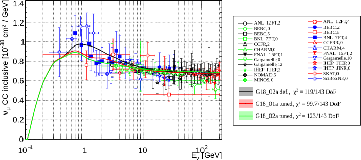
(a) Comparison of $\nu_{\mu}$ CC Inclusive cross-section data against against the default and tuned CMC.

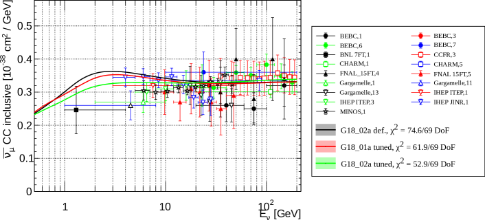
(b) Comparison of $\bar{\nu}_{\mu}$ CC Inclusive cross-section data against against the default and tuned CMCs.

Figure 8: Best fit prediction impact on muon (anti)neutrino CC inclusive cross sections as a function of the neutrino energy ($E_{\nu}$). The associated predictions for the default G18_02a and tuned G18_02a and G18_02a are computed with GENIE v3.0.6. Predictions are compared against all the available data (anti)neutrino interactions on $H$, ²H and heavier targets. Both CMC have been tuned against some $H$, ²H data (filled markers). Each $\chi^{2}$ is computed using all data available. In Tab. 9, the $\chi^{2}$ values per dataset are specified.

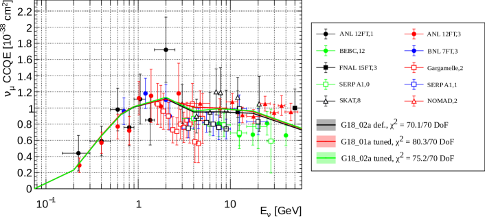
(a) Comparison of $\nu_{\mu}$ CC quasi-elastic cross-section data against the default and tuned CMCs.

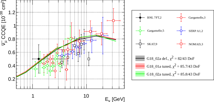
(b) Comparison of $\bar{\nu}_{\mu}$ CC quasi-elastic cross-section data against default and tuned CMCs.

Figure 9: Best fit prediction impact on muon (anti)neutrino CC quasi-elastic cross sections as a function of the neutrino energy ($E_{\nu}$). The associated predictions for the default G18_02a and tuned G18_02a and G18_02a are computed with GENIE v3.0.6. Predictions are compared against all the available data (anti)neutrino interactions on $H$, ²H and heavier targets. Bot CMC have been tuned against some $H$, ²H data (filled markers). Each $\chi^{2}$ is computed using all data available. In Tab. 9, the $\chi^{2}$ values per dataset are specified.

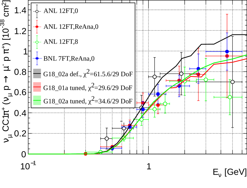
(a) Comparison of $\nu_{\mu}$ CC 1$\pi^{+}$ data on proton against the default and tuned CMCs.

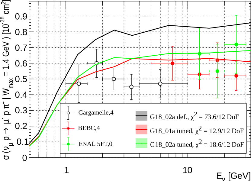
(b) Comparison of $\nu_{\mu}$ CC 1$\pi^{+}$ data on proton against the default and tuned CMCs. Experimental analysis impose a cut on $W$ at 1.4 GeV.

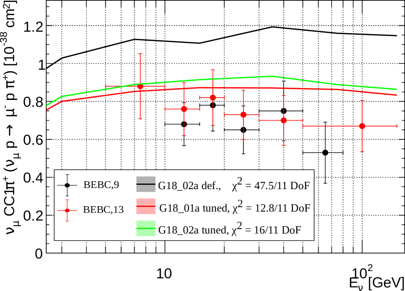
(c) Comparison of $\nu_{\mu}$ CC 1$\pi^{+}$ data on proton against the default and tuned CMCs. Experimental analysis impose a cut on $W$ at 2 GeV.

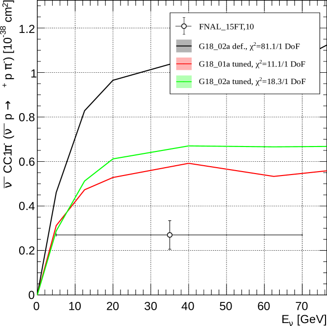
(d) Comparison of $\bar{\nu}_{\mu}$ CC 1$\pi^{+}$ data on proton against the default and tuned CMCs. The FNAL 15FT experiment applied a cut on $W$ at 1.9 GeV

Figure 10: Best fit prediction impact on muon neutrino on proton CC one pion production cross sections as a function of the neutrino energy ($E_{\nu}$). The associated predictions for the default G18_02a and tuned G18_02a and G18_02a are computed with GENIE v3.0.6. Experimental cuts are also applied to the predictions when needed. Predictions are compared against all the available data (anti)neutrino interactions on $H$, ²H and heavier targets. Both CMC have been tuned against some $H$, ²H data (filled markers). Each $\chi^{2}$ is computed using all data available. In Tab. 9, the $\chi^{2}$ values per dataset are specified.

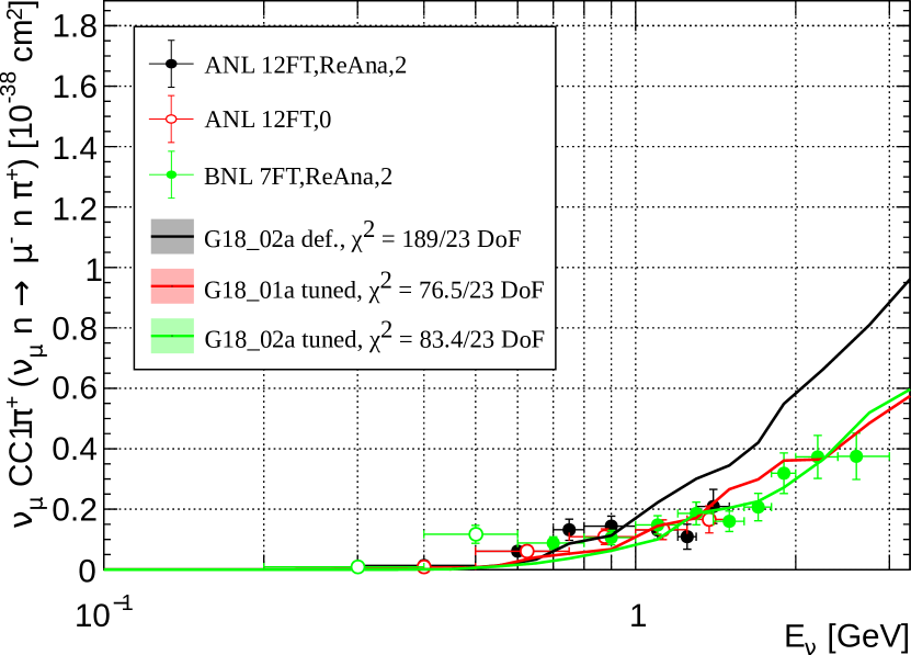
(a) Comparison of $\nu_{\mu}$ CC 1$\pi^{+}$ data on neutron against the default and tuned CMCs.

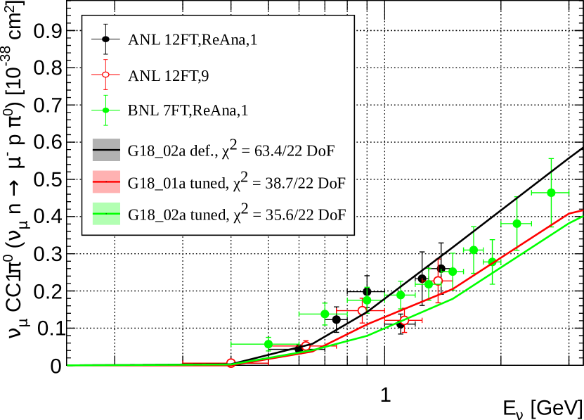
(b) Comparison of $\nu_{\mu}$ CC 1$\pi^{0}$ data on neutron against the default and tuned CMCs.

Figure 11: Best fit prediction impact on muon neutrino on neutron CC one pion production cross sections as a function of the neutrino energy ($E_{\nu}$). The associated predictions for the default G18_02a and tuned G18_02a and G18_02a are computed with GENIE v3.0.6. Predictions are compared against the original and reanalized ANL 12FT and BNL 7FT data [68, 67]. Only reanalized data with $E_{\nu}>0.5$ GeV is used in the tune (filled markers). Each $\chi^{2}$ is computed using all data available.

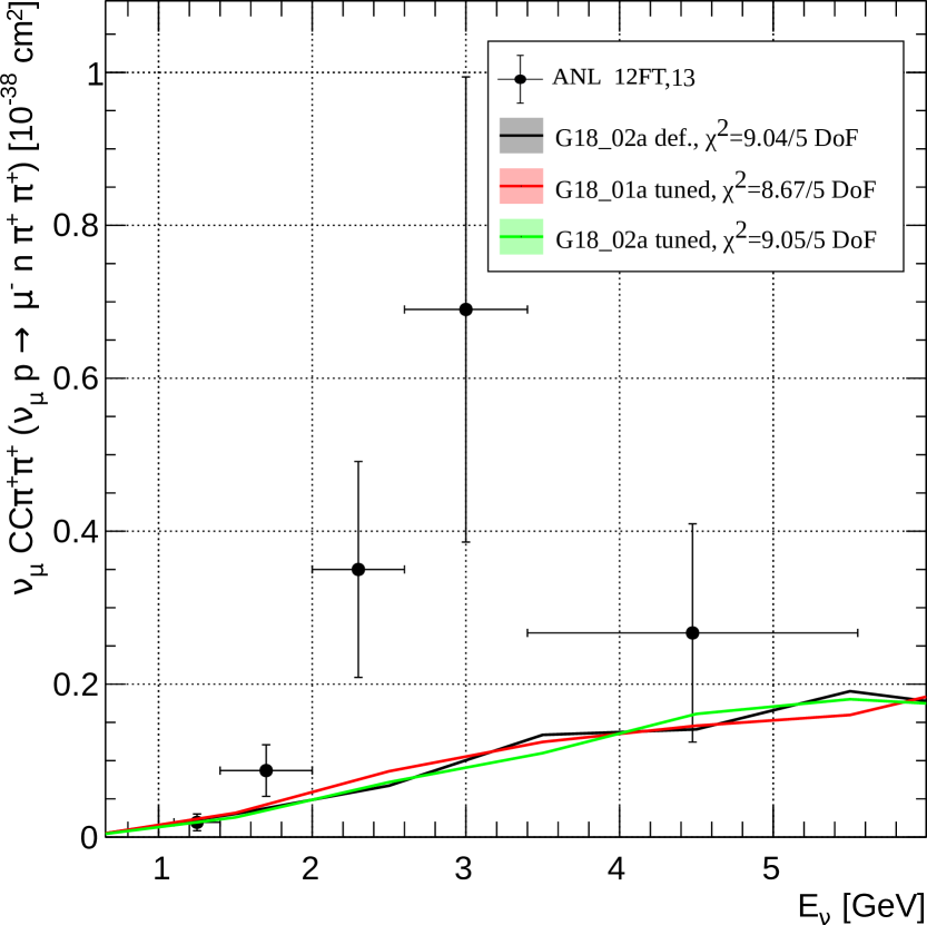
(a) Comparison of $\nu_{\mu}$ CC 2$\pi^{+}$ data on proton.

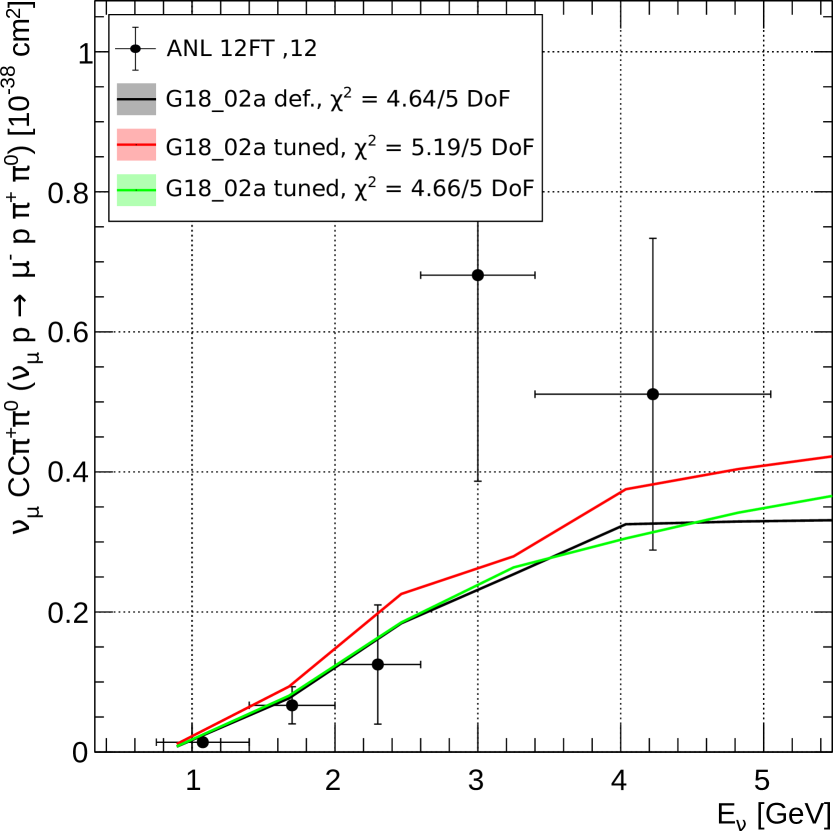
(b) Comparison of $\nu_{\mu}$ CC $\pi^{+}\pi^{0}$ data on proton.

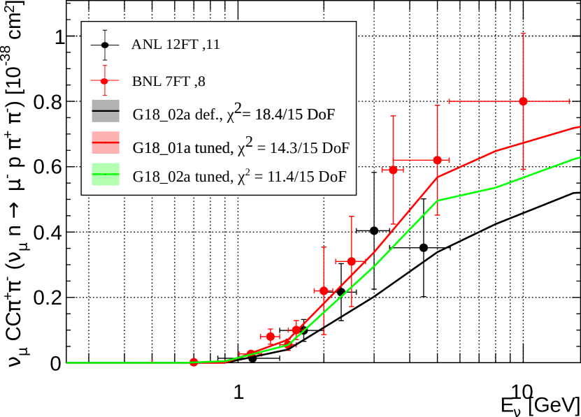
(c) Comparison of $\nu_{\mu}$ CC $\pi^{+}\pi^{-}$ data on neutron.

Figure 12: Best fit prediction impact on muon neutrino CC two-pion production cross sections as a function of the neutrino energy ($E_{\nu}$). The comparisons to two-pion production data are shown against the default and tuned CMCs. The associated predictions for the default G18_02a and tuned G18_02a and G18_02a are computed with GENIE v3.0.6. Predictions are compared against ANL 12FT and BNL 7FT data.

For all CMCs the tune has the most impact on the SIS region. In the inclusive cross-section prediction, this translates into a decrease of both $\nu_{\mu}$ and $\bar{\nu}_{\mu}$ CC inclusive cross section in the 0.5-10 GeV region, see Fig. 8. At the same time, the cross section at higher neutrino energies has barely changed, respecting the constraints of high-energy data. The agreement with quasi-elastic data, included in the tune in order to constrain the fluxes of each experiment, remained the same, see Fig. 9.

As discussed in Sec. VI, this decrease of the inclusive cross section at the SIS region is driven mainly by one pion production data. The impact on one pion exclusive channels is shown for (anti)neutrino on proton, Fig. 10, and neutrino on neutron, Fig. 11. The reduction of the one pion production cross section for neutrino on proton and neutron shows an improvement on $\nu_{\mu}\text{CC}1\pi^{+}$, $\nu_{\mu}$ and $\nu_{\mu}\text{CC}1\pi^{-}$ and $\nu_{\mu}\text{CC}1\pi^{0}$ channels when comparing it with the available data.

Two pion production exclusive cross sections are summarized in Fig. 12. This is the first time that two pion production data are used to tune the SIS region, allowing the $R_{\nu p}^{\text{CC}2\pi}$ and $R_{\nu n}^{\text{CC}2\pi}$ parameters to be constrained. In this case, the two pion exclusive cross section was underestimated by the default tune. For this particular exclusive process, comparisons are made against $\nu_{\mu}\text{CC}\pi^{+}\pi^{+}$, $\nu_{\mu}\text{CC}\pi^{+}\pi^{0}$ and $\nu_{\mu}\text{CC}\pi^{+}\pi^{-}$ data. The shape of the GENIE prediction for the $\nu_{\mu}\text{CC}\pi^{+}\pi^{+}$ and $\nu_{\mu}\text{CC}\pi^{+}\pi^{0}$ channels differs strongly from data, and the models are not able to accommodate this behaviour. However, the agreement with $\nu_{\mu}\text{CC}\pi^{+}\pi^{-}$ data has improved by increasing the cross section with respect to the default cross-section model.

Despite the tensions between inclusive and exclusive data discussed in Sec. IV.2, the overall agreement for both cross-section model constructions has improved, see Tab. 9. Particularly, $\bar{\nu}_{\mu}$ CC inclusive predictions show better agreement after the tune, and the same is observed for $\nu_{\mu}$ CC inclusive predictions for the G18_01a free nucleon tune. Although the impact on the cross-section prediction of the tune is similar for the existing configurations, the response of each model at the parameter level is not expected to be the same. Therefore, each tune is strongly affected by how the model is able to accommodate the data by modifying the tuned parameters. This reflects on the $R_{m}$ parameters and $W_{\text{cut}}$ which best fit values are incompatible in some cases, such as for $R_{\nu n}^{\text{CC}1\pi}$, see Tab. 6. Particularly, the behaviour of $R_{\nu p}^{\text{CC}1\pi}$ on the G18_02a(/b) tune was showing preference for nonphysical regions of the tune, forcing us to fix this value to $R_{\nu p}^{\text{CC}1\pi}=0.008$. On the other hand, the remaining parameters, such as $M_{A}^{\text{RES}}$ and $M_{A}^{\text{QE}}$, show agreement between the tunes and respect the applied priors.

VI.3 Parameter error estimation

An estimate of the parameter uncertainties is shown in Tab. 6. For each parameter of interest allowed to float in the fit, the table shows the range of values that satisfies the condition ${\Delta\chi^{2}_{\text{profile}}(\theta_{i})<\Delta\chi^{2}_{\text{critical}}=1}$. In the previous expression, the function $\Delta\chi^{2}_{\text{profile}}(\theta_{i})$ is constructed by fixing $\theta_{i}$ to a desired value and minimising the quantity $\Delta\chi^{2}(\bm{\theta},\bm{f})=\chi^{2}(\bm{\theta},\bm{f})-\chi^{2}_{\text{min}}$ with respect to all other parameters that were allowed to float in the fit. See Sec. V.1 for the definition of $\chi^{2}(\bm{\theta},\bm{f})$. The constant $\chi^{2}_{\text{min}}$ corresponds to the minimum value of $\chi^{2}(\bm{\theta},\bm{f})$ obtained from the global fit. The $\Delta\chi^{2}_{\text{profile}}(\theta_{i})$ functions we derive from our analysis are shown in Fig. 13, for all parameters $\theta_{i}$ that were allowed to float in the fit, up to $\Delta\chi^{2}_{\text{profile}}$ values of 2. Particularly, $W_{\text{cut}}$ is fixed to the best fit value during this approach, as it is an ad-hoc parameter introduced by the generator: by fixing it, its uncertainty will be reflected on the other parameters. It is important to emphasize that the uncertainties quoted relate only to $\Delta\chi^{2}_{\text{critical}}=1$. However, this region is strongly determined by the underlying model used in the tune.

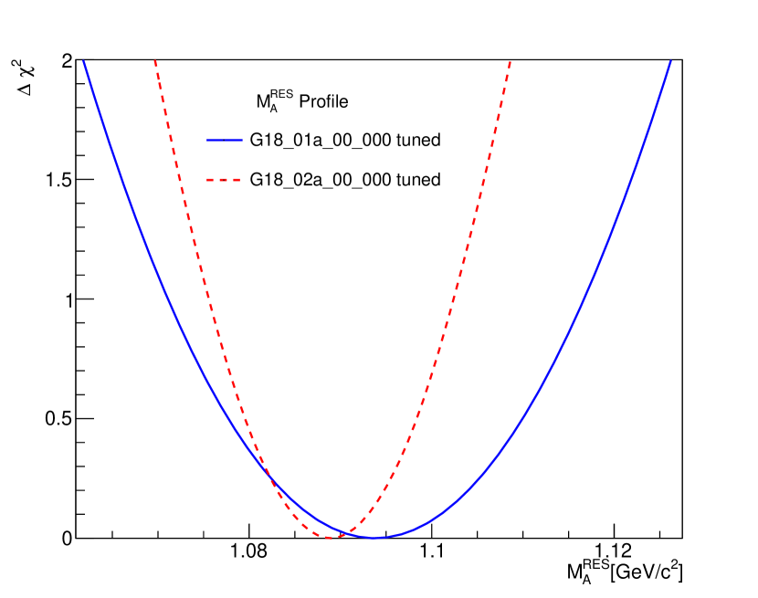
(a) Profile for $M_{A}^{\text{RES}}.$

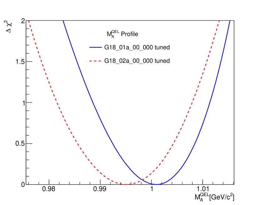
(b) Profile for $M_{A}^{\text{QE}}.$

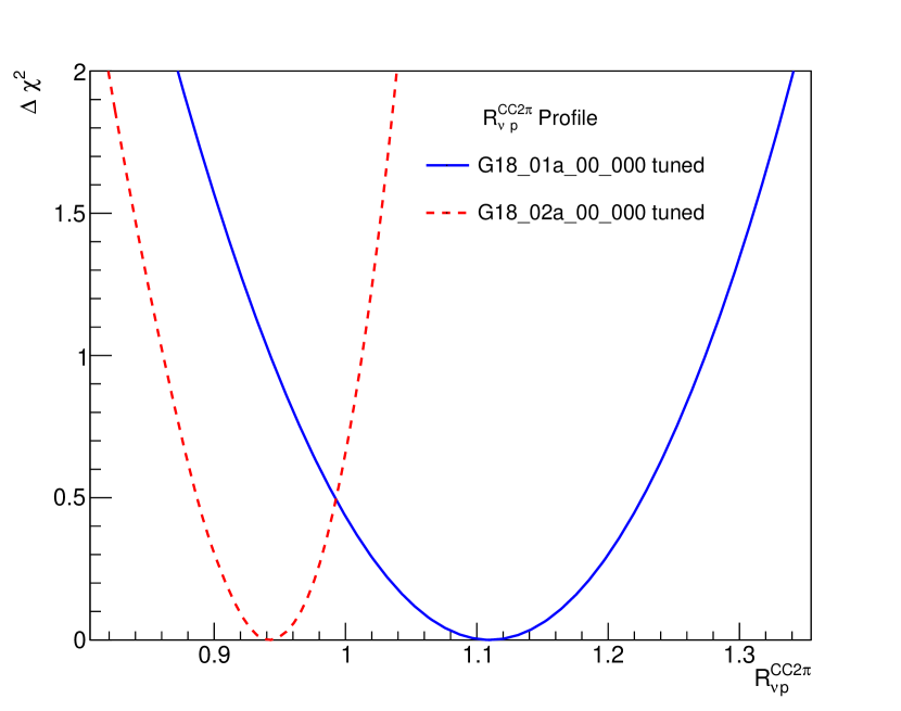
(c) Profile for $R_{\nu p}^{\text{CC}2\pi}$.

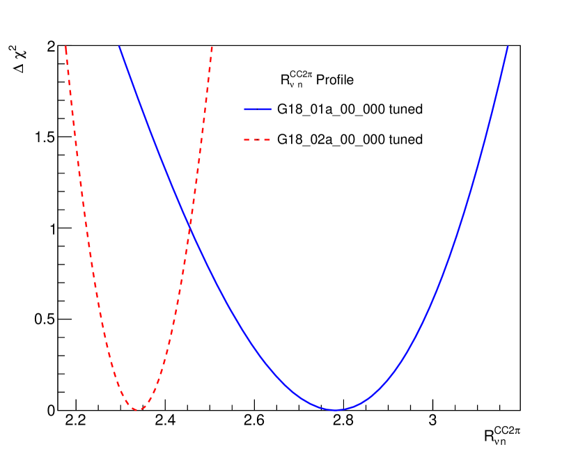
(d) Profile for $R_{\nu n}^{\text{CC}2\pi}$.

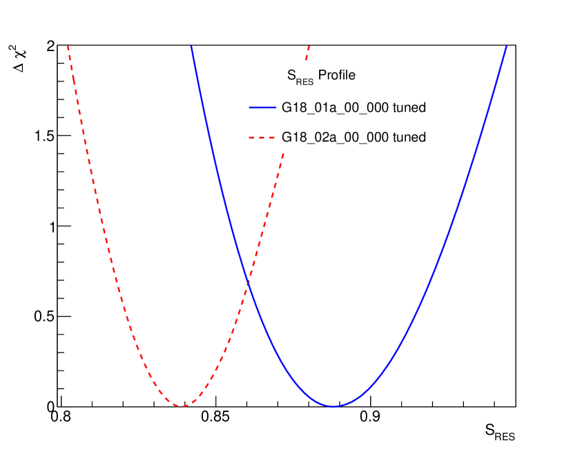
(e) Profile for $S_{\text{RES}}$.

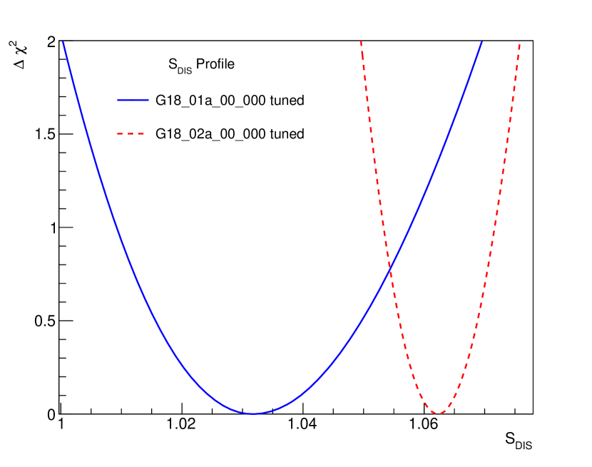
(f) Profile for $S_{\text{DIS}}$.

Figure 13: $\Delta\chi^{2}_{\text{profile}}(\theta_{i})$ functions obtained fixing the parameter under study and minimizing $\Delta\chi^{2}(\theta_{i})=\chi^{2}(\vec{\theta},\vec{f})-\chi^{2}_{\text{min}}$ respect the other parameters in the tune. The profiles for both tunes are shown for each case. The G18_02a profiles show that this configuration is less able to accommodate in the model variations on each parameter best fit values.

A covariance matrix is also obtained through the inversion of the the Hessian of the log-likelihood function at the best-fit parameter point. The corresponding correlation matrices are presented in Tab. 8(a) and Tab. 8(b) for the tunes of all 4 different cross-section model constructions used in this work (see the correlation matrices in Fig. 14 and Fig. 15 for a graphical interpretation). An example of the propagation of model uncertainties from the Professor output to the GENIE Comparisons framework is shown in Fig. 17.

	$M_{A}^{\text{RES}}$	$M_{A}^{\text{QE}}$	$R_{\nu p}^{\text{CC}1\pi}$	$R_{\nu p}^{\text{CC}2\pi}$	$R_{\nu n}^{\text{CC}1\pi}$	$R_{\nu n}^{\text{CC}2\pi}$	$S_{\text{RES}}$	$S_{\text{DIS}}$
$M_{A}^{\text{RES}}$	5.3E-4	-7E-5	5E-5	-8E-4	2.2E-4	-2.4E-3	-4.3E-4	-9E-5
$M_{A}^{\text{QE}}$	-7E-5	1.2E-4	-6E-5	-1.2E-4	-5E-5	-7.6E-4	1.2E-4	1E-5
$R_{\nu p}^{\text{CC}1\pi}$	5E-5	-6E-5	9.3E-4	-1.6E-3	2.6E-4	5.4E-4	-2.8E-4	-6E-5
$R_{\nu p}^{\text{CC}2\pi}$	-8E-4	-1.2E-4	-1.6E-3	2.7E-2	2.0E-5	-2.5E-4	2E-3	-6.2E-4
$R_{\nu n}^{\text{CC}1\pi}$	2.2E-4	-5E-5	2.6E-4	2E-5	7.1E-4	2.3E-3	-5.3E-4	-8E-5
$R_{\nu n}^{\text{CC}2\pi}$	-2.4E-3	-7.6E-4	5.4E-4	-2.5E-4	2.3E-3	9.6E-2	-2.5E-3	-1.4E-3
$S_{\text{RES}}$	-4.3E-4	1.2E-4	-2.8E-4	2E-3	-5.3E-4	-2.5E-3	1.3E-3	1.8E-4
$S_{\text{DIS}}$	-9E-5	1E-5	-6E-5	-6.2E-4	-8E-5	-1.4E-3	1.8E-4	5.1E-4

(a) G18_01a(/b) covariance matrix.

	$M_{A}^{\text{RES}}$	$M_{A}^{\text{QE}}$	$R_{\nu p}^{\text{CC}2\pi}$	$R_{\nu n}^{\text{CC}1\pi}$	$R_{\nu n}^{\text{CC}2\pi}$	$S_{\text{RES}}$	$S_{\text{DIS}}$
$M_{A}^{\text{RES}}$	1.7E-4	2.0E-5	-1.9E-4	-6.0E-5	4.4E-4	6.0E-5	-4.0E-5
$M_{A}^{\text{QE}}$	2.0E-5	1.8E-4	-7.0E-5	3.0E-5	-2.1E-4	1.5E-4	1.0E-5
$R_{\nu p}^{\text{CC}2\pi}$	-1.9E-4	-7.0E-5	5.5E-3	1.5E-4	-2.4E-3	-6.9E-4	3.0E-5
$R_{\nu n}^{\text{CC}1\pi}$	-6.0E-5	3.0E-5	1.5E-4	1.1E-4	-1.0E-4	-6.0E-5	6.0E-5
$R_{\nu n}^{\text{CC}2\pi}$	4.4E-4	-2.1E-4	-2.4E-3	-1.0E-4	1.3E-2	2.3E-4	-8.0E-5
$S_{\text{RES}}$	6.0E-5	1.5E-4	-6.9E-4	-6.0E-5	2.3E-4	6.0E-4	-4.0E-5
$S_{\text{DIS}}$	-4.0E-5	1.0E-5	3.0E-5	6.0E-5	-8.0E-5	-4.0E-5	8.0E-5

(b) G18_02a(/b) covariance matrix.

Table 8: Parameter covariance matrices extracted the GENIE fit for the tuned CMCs.

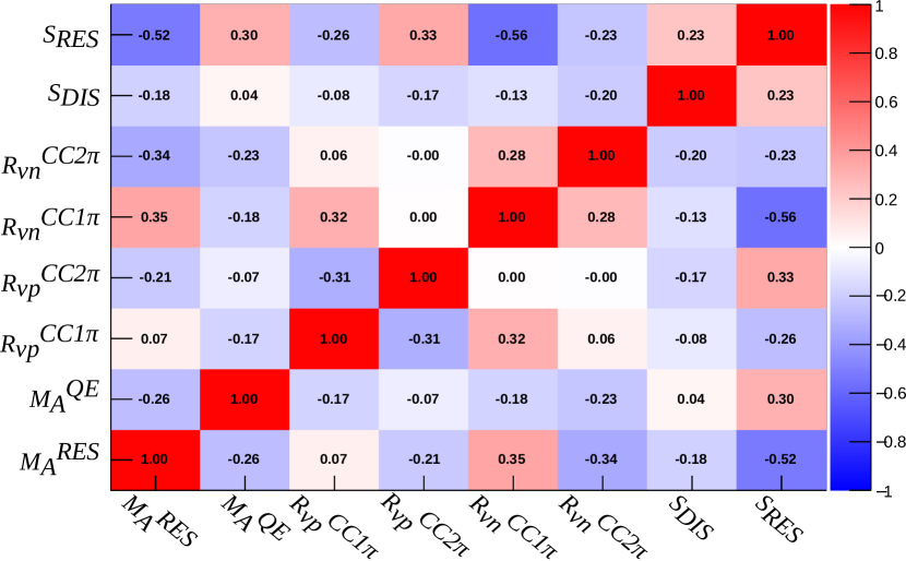
Figure 14: Parameter correlation matrix from the GENIE fit using the G18_01a(/b) CMC correlation matrix.

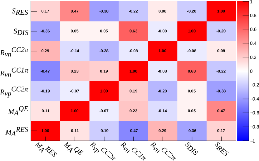
Figure 15: Parameter correlation matrix from the GENIE fit using the G18_02a(/b) CMC correlation matrix.

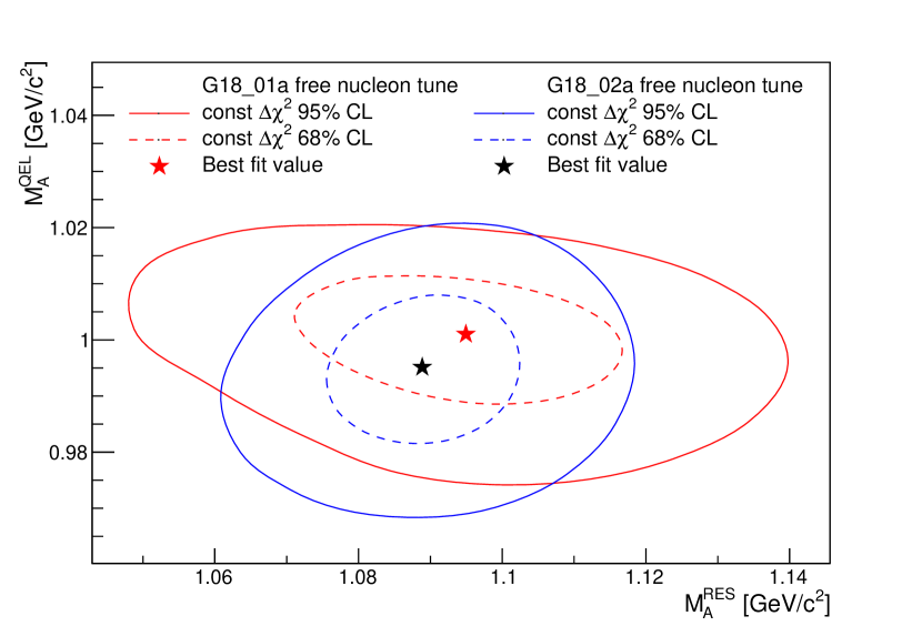
(a) Contour $M_{A}^{\text{RES}}$ vs $M_{A}^{\text{QE}}$

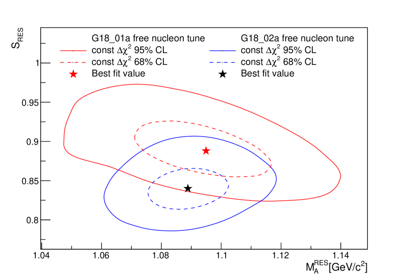
(b) Contour $M_{A}^{\text{RES}}$ vs $S_{\text{RES}}$

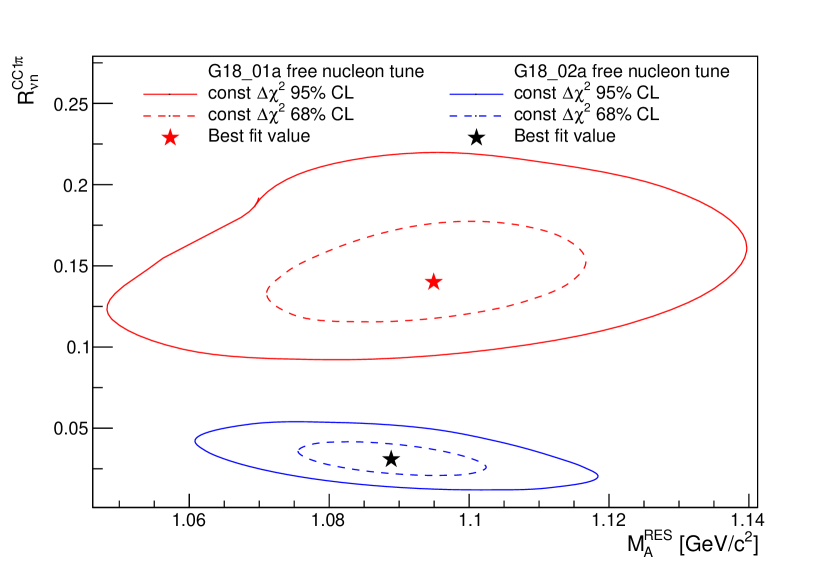
(c) Contour $M_{A}^{\text{RES}}$ vs $R_{\nu n}^{\text{CC}1\pi}$

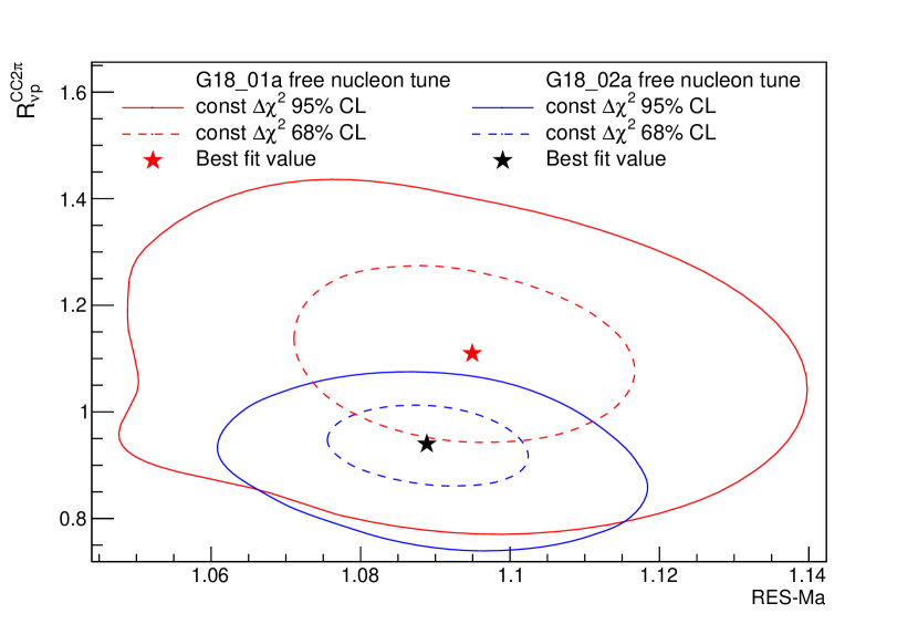
(d) Contour $M_{A}^{\text{RES}}$ vs $R_{\nu p}^{\text{CC}2\pi}$

Figure 16: Joint $\Delta\chi^{2}_{\text{profile}}(\theta_{i},\theta_{j})$ functions obtained fixing the two parameters under study and minimizing $\Delta\chi^{2}(\vec{\theta},\vec{f})$ respect the other parameters in the tune. The contours for both tunes are shown for each case as well as the best fit values of each tune.

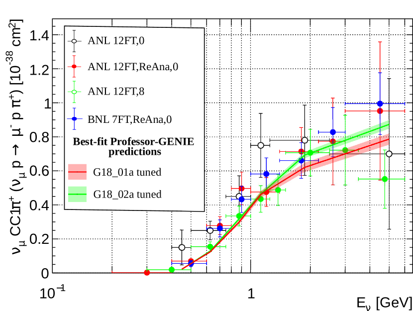
(a) $\nu_{\mu}\text{CC}1\pi^{+}$ comparison.

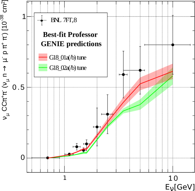
(b) $\nu_{\mu}\text{CC}\pi^{+}\pi^{-}$ comparison.

Figure 17: Comparisons of neutrino data against predictions obtained from the Professor-GENIE parametrization at the best-fit value. The uncertainties of the tune are propagated to the prediction considering the full covariance matrix.

Joint $\Delta\chi^{2}_{\text{profile}}(\theta_{i},\theta_{j})$ functions, constructed by fixing two parameters at a grid of values and minimizing and $\Delta\chi^{2}(\bm{\theta},\bm{f})$ with respect to all other new parameters, are shown in Fig.  16 for selected sets of parameters. In Figs.16, we can see that the coverage of the parameter space for the 68% and 95% confidence level lines is wider for the G18_01a(/b) tunes. This characteristic is again not related with how well we can constrain the parameters from the data, but with the capability of the models to accommodate this data in each model implementation.

VII Conclusions

GENIE has released a number of comprehensive model configurations (CMCs) which consist of different modelling aspects combined altogether. In previous GENIE versions, there was a preferred default comprehensive model which failed to describe both inclusive and exclusive channels due to unresolved tensions between the data. These tensions, which are crucial to understand for the new generation of neutrino experiments, motivated a careful investigation and retune of the bare-nucleon cross-section model for all GENIE comprehensive models available in GENIE v3. Best-fit values and correlations for several parameters influencing the GENIE bare-nucleon cross sections are released in this paper.

In GENIE v3, we focus on improving understanding of the SIS region by tuning the GENIE CMC predictions on hydrogen and deuterium data from ANL 12FT, BNL 7FT, BEBC and FNAL 15FT bubble chamber experiments. The tuning of the non-resonant background takes a central stage in this work in order to remove double counting issues. The SIS region has been tuned against $\nu_{\mu}$ and $\bar{\nu}_{\mu}$ CC inclusive, quasi-elastic, one pion and two pion integrated cross sections as a function of $E_{\nu}$. Quasi-elastic data has been introduced to the fit to better constrain the flux of each experiment.

The global fit is able to describe both inclusive and exclusive cross sections simultaneously. Tensions between inclusive and exclusive data have been re-encountered, and, as a consequence, the inclusive cross section at the 1–10 GeV energy region decreased with respect to the historical default value. The systematic treatment of correlations between datasets and the inclusion of priors were crucial to address tensions. After the tune, GENIE predictions of one pion production cross sections on free nucleons ($\nu_{\mu}$CC p$\pi^{+}$, n$\pi^{+}$, p$\pi^{0}$ and p$\pi^{+}\pi^{-}$) show a decrease in the non-resonant background contribution, improving the agreement with the data. The prediction for two pion production mechanisms is also in better agreement with data for the $\nu_{\mu}n\rightarrow\mu^{-}p\pi^{+}\pi^{-}$ channel by increasing the two pion production non-resonant background contribution.

VIII Acknowledgements

We would like to thank Andy Buckley (University of Glasgow, UK) and Holger Schultz (Institute of Particle Physics Phenomenology, University of Durham, UK) for their support interfacing the Professor tool with the software products that underpin the GENIE global analysis. We are also grateful with Luis Alvarez-Ruso for insightful discussions and the review of this paper. We would like to thank the CC-IN2P3 Computing Center, as well as the Particle Physics Department at Rutherford Appleton Laboratory for providing computing resources and for their support. This work, as well as the ongoing development of several other GENIE physics tunes was enabled through a PhD studentship funded by STFC through LIV.DAT, the Liverpool Big Data Science Centre for Doctoral Training (project reference: 2021488). The initial conceptual and prototyping work for the development of the GENIE / Professor interfaces, as well as for the development of the GENIE global analysis framework that, currently, underpins several analyses, was supported in part through an Associateship Award by the Institute of Particle Physics Phenomenology, University of Durham.

This document was prepared by the GENIE collaboration using the resources of the Fermi National Accelerator Laboratory (Fermilab), a U.S. Department of Energy, Office of Science, HEP User Facility. Fermilab is managed by Fermi Research Alliance, LLC (FRA), acting under Contract No. DE-AC02-07CH11359.

		$\mathbf{\chi^{2}}$ values for G18_01a		$\mathbf{\chi^{2}}$ values for G18_02a
Dataset	$\mathbf{N_{DOF}}$	default	Best Fit	default	Best Fit
$\nu_{\mu}$ CC Inclusive
BNL 7FT [44]	13	11.1	9.95	14.7	7.75
BEBC  [42]	3	0.215	0.101	0.067	0.045
FNAL 15FT  [74, 47]	10	3.85	3.92	4.04	4.98
$\bar{\nu}_{\mu}$ CC Inclusive
BEBC [42, 31, 43]	11	11.17	11.5	9.79	9.8
BNL 7FT [53]	1	1.83	1.51	1.96	0.827
FNAL 15FT [49, 54]	13	3.86	4.12	4.32	4.13
$\nu_{\mu}n\rightarrow\mu^{-}n\pi^{+}$
ANL 12FT [67]	5	11.6	9.88	27.3	14.3
ANL 12FT,ReAna [68]	7	31.3	21.0	48.8	25.2
BNL 7FT,ReAna [68]	11	103	45.7	112	43.9
$\nu_{\mu}p\rightarrow\mu^{-}p\pi^{+}$
ANL 12FT,ReAna  [68]	8	11	8.71	17.8	9.64
BNL 7FT,ReAna  [68]	7	6.16	3.11	9.71	3.9
BEBC [70, 58, 72]	15	33.98	15.9	82.6	21.0
FNAL [77]	3	1.11	0.74	2.87	0.66
$\nu_{\mu}n\rightarrow\mu^{-}p\pi^{0}$
ANL 12FT [67]	5	4.89	4.98	7.57	4.63
ANL 12FT,ReAna [68]	7	12.6	12.0	17.4	11.5
BNL 7FT,ReAna [68]	10	31.8	21.7	38.4	19.4
$\nu_{\mu}p\rightarrow\mu^{-}n\pi^{+}\pi^{+}$
ANL 12FT [75]	5	9.23	8.67	9.04	9.05
$\nu_{\mu}p\rightarrow\mu^{-}p\pi^{+}\pi^{0}$
ANL 12FT [75]	5	4.28	5.19	4.64	4.66
$\nu_{\mu}n\rightarrow\mu^{-}p\pi^{+}\pi^{-}$
ANL 12FT [75]	5	8.24	8.36	8.09	4.95
BNL 7FT [35]	10	11.6	5.96	10.3	6.46
$\nu_{\mu}$ CC QE
ANL 12FT [57, 29]	15	11.7	12.2	11.75	11.58
BNL 7FT [62]	4	6.88	6.91	6.98	7.58
BEBC [58]	5	8.18	9.45	8.21	9.54
FNAL [59]	2	0.886	0.951	0.992	0.893
$\bar{\nu}_{\mu}$ CC QE
BNL 7FT [53]	1	0.161	0.135	0.078	0.106
Total	182	400.6	229.5	459.4	236.5

Table 9: Contributions to the default and best fit $\chi^{2}$ for the datasets included. The data points with ${E_{\nu}<0.5}$ GeV, a total of 10 points, are considered in the $\chi^{2}$ calculations of this table, but were not used in the fit. For the calculation of the $\chi^{2}$, the covariance matrix between the datasets is used instead of Eq. V.4, which incorporates nuisance parameters which are not implemented in GENIE. This explains the difference when comparing with the $\chi^{2}$ out of Professor from Tab. 6.

Experiment	Tag	Ref.
$\nu_{\mu}$ CC Inclusive
ANL 12 FT	ANL 12 FT,2	[29]
BEBC	BEBC,0	[30]
BEBC	BEBC,5	[31]
BNL 7FT	BNL 7FT,0	[32]
CCFR	CCFR,2	[33]
CHARM	CHARM,0	[34]
FNAL 15FT	FNAL 15FT,1	[35]
Gargamelle	Gargamelle,0	[36]
Gargamelle	Gargamelle,12	[37]
IHEP_ITEP	IHEP_ITEP,2	[38]
NOMAD	NOMAD,5	[39]
MINOS	MINOS,0	[40]
ANL 12FT	ANL 12FT,4	[41]
BEBC	BEBC,2	[42]
BEBC	BEBC,8	[43]
BNL 7FT	BNL 7FT,4	[44]
CCFRR	CCFRR,0	[45]
CHARM	CHARM,4	[46]
FNAL 15FT	FNAL 15FT,2	[47]
Gargamelle	Gargamelle,10	[48]
IHEP_ITEP	IHEP_ITEP,0	[49]
IHEP_JINR	IHEP_JINR,0	[50]
SKAT	SKAT,0	[51]
SciBooNE	SciBooNE,0	[52]
$\bar{\nu}_{\mu}$ CC Inclusive
BEBC	BEBC,1	[30]
BEBC	BEBC,6	[31]
BNL 7FT	BNL 7FT,1	[53]
CHARM	CHARM,1	[34]
FNAL 15FT	FNAL 15FT,4	[54]
Gargamelle	Gargamelle,1	[36]
Gargamelle	Gargamelle,13	[37]
IHEP_ITEP	IHEP_ITEP,3	[38]
MINOS	MINOS,1	[40]
BEBC	BEBC,3	[42]
BEBC	BEBC,7	[43]
CCFR	CCFR,3	[33]
CHARM	CHARM,5	[46]
FNAL 15FT	FNAL 15FT,5	[49]
Gargamelle	Gargamelle,11	[55]
IHEP_ITEP	IHEP_ITEP,1	[56]
IHEP_JINR	IHEP_JINR,1	[50]

Experiment	Tag	Ref.
$\nu_{\mu}$ CC Quasi-elastic
ANL 12FT	ANL 12FT,1	[57]
BEBC	BEBC,12	[58]
FNAL 15FT	FNAL 15FT,3	[59]
SERP A1	SERP A1,0	[60]
SKAT	SKAT,8	[61]
ANL 12FT	ANL 12FT,3	[29]
BNL 7FT	BNL 7FT,3	[62]
Gargamelle	Gargamelle,2	[63]
SERP A1	SERP A1,1	[64]
NOMAD	NOMAD,2	[39]
$\bar{\nu}_{\mu}$ CC Quasi-elastic
BNL 7FT	BNL 7FT,2	[53]
Gargamelle	Gargamelle,5	[65]
SKAT	SKAT,9	[61]
Gargamelle	Gargamelle,3	[63]
SERP A1	SERP A1,2	[64]
NOMAD	NOMAD,3	[39]
$\nu_{\mu}\text{CC}1\pi^{+}$ ($\nu_{\mu}p\rightarrow\mu^{-}p\pi^{+}$)
ANL 12FT	ANL 12FT,0	[66]
ANL 12FT	ANL 12FT,ReAna,0	[67]
ANL 12FT	ANL 12FT,8	[68]
BNL 7FT	BNL 7FT,ReAna,0	[68]
Gargamelle	Gargamelle,4	[69]
BEBC	BEBC,4	[70]
FNAL 15FT	FNAL 15FT,0	[71]
BEBC	BEBC,9	[72]
BEBC	BEBC,13	[58]
$\bar{\nu}_{\mu}\text{CC}1\pi^{-}$ ($\bar{\nu}p\rightarrow\mu^{+}p\pi^{-}$)
FNAL 15FT	FNAL 15FT,10	[73]
$\nu_{\mu}\text{CC}1\pi^{+}$ ($\nu n\rightarrow\mu^{-}n\pi^{+}$)
ANL 12FT	ANL 12FT,ReAna,2	[68]
BNL 7FT	BNL 7FT,ReAna,2	[68]
ANL 12FT	ANL 12FT,10	[67]
$\nu_{\mu}\text{CC}1\pi^{0}$ ($\nu n\rightarrow\mu^{-}p\pi^{0}$)
ANL 12FT	ANL 12FT,ReAna,1	[68]
BNL 7FT	BNL 7FT,ReAna,1	[68]
ANL 12FT	ANL 12FT,9	[67]
$\nu_{\mu}\text{CC}1\pi^{+}\pi^{+}$ ($\nu p\rightarrow\mu^{-}n\pi^{+}\pi^{+}$)
ANL 12FT	ANL 12FT,13	[75]
$\nu_{\mu}\text{CC}1\pi^{+}\pi^{0}$ ($\nu p\rightarrow\mu^{-}p\pi^{+}\pi^{0}$)
ANL 12FT	ANL 12FT,12	[75]
$\nu_{\mu}\text{CC}1\pi^{+}\pi^{-}$ ($\nu n\rightarrow\mu^{-}p\pi^{+}\pi^{-}$)
ANL 12FT	ANL 12FT,12	[75]
BNL 7FT	BNL 7FT,8	[74]

Table 10: Summary of data used for comparisons in Figs. 6, 7(a), 7(b), 8, 9, 10, 12, 11 and 17. This table links the experiment and the tag used for the legend in each plot to the corresponding reference.

References

- Andreopoulos et al. [2010] C. Andreopoulos et al., The GENIE Neutrino Monte Carlo Generator, Nucl. Instrum. Meth. A 614, 87 (2010), arXiv:0905.2517 [hep-ph] .
- Buckley et al. [2010a] A. Buckley, H. Hoeth, H. Lacker, H. Schulz, and J. E. von Seggern, Systematic event generator tuning for the LHC, Eur. Phys. J. C 65, 331 (2010a), arXiv:0907.2973 .
- Schulz et al. [2020] H. Schulz et al., Professor web page (2020), https://professor.hepforge.org.
- Rodrigues et al. [2016] P. Rodrigues, C. Wilkinson, and K. McFarland, Constraining the GENIE model of neutrino-induced single pion production using reanalyzed bubble chamber data 10.1140/epjc/s10052-016-4314-3 (2016), arXiv:1601.01888 .
- Rein and Sehgal [1981] D. Rein and L. M. Sehgal, Neutrino-excitation of baryon resonances and single pion production, Ann. Phys. 133, 79 (1981).
- Kuzmin et al. [2004] K. S. Kuzmin, V. V. Lyubushkin, and V. A. Naumov, Lepton polarization in neutrino–nucleon interactions, Mod. Phys. Lett. A19, 2815 (2004), Phys. Part. Nucl. 35, S133 (2004), arXiv:hep-ph/0312107 [hep-ph] .
- Kuzmin et al. [2005] K. S. Kuzmin, V. V. Lyubushkin, and V. A. Naumov, Extended Rein-Sehgal model for tau lepton production, Nucl. Phys. B (Proc. Suppl.) 139, 158 (2005), arXiv:hep-ph/0408106 [hep-ph] .
- Berger and Sehgal [2007] C. Berger and L. M. Sehgal, Lepton mass effects in single pion production by neutrinos, Phys. Rev. D76, 113004 (2007), [Erratum-ibid. D 77, 059901(E) (2008)], arXiv:0709.4378 [hep-ph] .
- Bodek and Yang [2002] A. Bodek and U. Yang, Modeling deep inelastic cross sections in the few GeV region, Nucl. Phys. B (Proc. Suppl.) 112, 70 (2002).
- Yang et al. [2009] T. Yang, C. Andreopoulos, H. Gallagher, K. Hoffmann, and P. Kehayias, A Hadronization Model for Few-GeV Neutrino Interactions, Eur. Phys. J. C63, 1 (2009), arXiv:0904.4043 [hep-ph] .
- Mandula et al. [1969] J. Mandula, C. Rebbi, R. Slansky, J. Weyers, and G. Zweig, Duality and the hadron spectrum, Phys. Rev. Lett. 22, 1147 (1969).
- Grässler et al. [1983] H. Grässler et al., Multiplicities of secondary hadrons produced in and charged current interactions, Nucl. Phys. B 223, 269 (1983).
- Ahrens et al. [1987] L. Ahrens et al., Measurement of neutrino-proton and antineutrino-proton elastic scattering, Phys. Rev. D 35, 785 (1987).
- Llewellyn Smith [1972] C. Llewellyn Smith, Neutrino reactions at accelerator energies, Phys. Rept. 3, 261 (1972).
- Rein and Sehgal [1983] D. Rein and L. M. Sehgal, Coherent Production in Neutrino Reactions, Nucl. Phys. B 223, 29 (1983).
- Kovalenko [1990] S. Kovalenko, Quasielastic neutrino production of charmed baryons from the point of view of local duality, Sov. J. Nucl. Phys. 52, 934 (1990).
- Aivazis et al. [1991] M. A. G. Aivazis, W.-K. Tung, and F. I. Olness, Next-to-leading order QCD formulation of deep inelastic scattering, in Proceedings, The Vancouver Meeting, Particles & Fields’91: Vancouver, Canada, August 18–22, 1991 (1991) pp. 663–665, arXiv:hep-ph/9302305 [hep-ph] .
- Bodek and Ritchie [1981] A. Bodek and J. L. Ritchie, Fermi-motion effects in deep-inelastic lepton scattering from nuclear targets, Phys. Rev. D 23, 1070 (1981).
- Rein [1986] D. Rein, Diffractive pion production in neutrino reactions, Nucl. Phys. B 278, 61 (1986).
- Pais [1971] A. Pais, Weak interactions at high energies, Annals of Physics 63, 361 (1971).
- Rafi Alam et al. [2010] M. Rafi Alam, I. Ruiz Simo, M. Sajjad Athar, and M. J. Vicente Vacas, Weak Kaon Production off the Nucleon, Phys. Rev. D 82, 033001 (2010), arXiv:1004.5484 [hep-ph] .
- Dytman et al. [2021] S. Dytman, Y. Hayato, R. Raboanary, J. Sobczyk, J. Tena-Vidal, and N. Vololoniaina, Comparison of validation methods of simulations for final state interactions in hadron production experiments (2021), arXiv:2103.07535 [hep-ph] .
- Agostinelli et al. [2003] S. Agostinelli et al., Geant4—a simulation toolkit, Nucl. Instrum. and Meth. in Phys. Res. A 506, 250 (2003).
- Heikkinen et al. [2003] A. Heikkinen, N. Stepanov, and J. P. Wellisch, Bertini intranuclear cascade implementation in GEANT4, eConf C0303241, MOMT008 (2003), arXiv:nucl-th/0306008 .
- Mancusi et al. [2015] D. Mancusi, A. Boudard, J. Carbonell, J. Cugnon, J.-C. David, and S. Leray, Improving the description of proton-induced one-nucleon removal in intranuclear-cascade models, Phys. Rev. C 91, 034602 (2015), arXiv:1411.4562 [nucl-th] .
- Nieves et al. [2011] J. Nieves, I. R. Simo, and M. J. V. Vacas, Inclusive charged-current neutrino-nucleus reactions, Phys. Rev. C 83, 045501 (2011).
- Schwehr et al. [2017] J. Schwehr, D. Cherdack, and R. Gran, Genie implementation of ific valencia model for qe-like 2p2h neutrino-nucleus cross section (2017), arXiv:1601.02038 [hep-ph] .
- Meyer et al. [2016] A. S. Meyer, M. Betancourt, R. Gran, and R. J. Hill, Deuterium target data for precision neutrino-nucleus cross sections, Phys. Rev. D 93, 113015 (2016), arXiv:1603.03048 [hep-ph] .
- Barish et al. [1977] S. J. Barish et al., Study of Neutrino Interactions in Hydrogen and Deuterium. 1. Description of the Experiment and Study of the Reaction , Phys. Rev. D16, 3103 (1977).
- Bosetti et al. [1977] P. C. Bosetti et al. (Aachen-Bonn-CERN-London-Oxford-Saclay), Total Cross Sections for Charged-Current Neutrino and anti-neutrino Interactions in BEBC in the Energy Range 20–200 GeV, Phys. Lett. B70, 273 (1977).
- Bosetti et al. [1982] P. Bosetti et al. (Aachen-Bonn-CERN-Democritos-London-Oxford-Saclay), Total cross-sections for and charged-current interactions between 20 and 200 GeV, Phys. Lett. B110, 167 (1982).
- Baltay et al. [1980] C. Baltay et al., Cross-sectons and scaling variable distributions of neutral and charged current neutrino nucleon interactions from a low-energy narrow band beam, Phys. Rev. Lett. 44, 916 (1980).
- Seligman [1997] W. G. Seligman, A Next-to-Leading Order QCD Analysis of Neutrino–Iron Structure Functions at the Tevatron, Ph.D. thesis, Nevis Labs, Columbia U. (1997).
- Jonker et al. [1981] M. Jonker et al. (CHARM), Experimental Study of Neutral-Current and Charged-Current Neutrino Cross Sections, Phys. Lett. B99, 265 (1981), [Erratum-ibid. B 100, 520 (1981)].
- Kitagaki et al. [1986] T. Kitagaki et al., Charged-current exclusive pion production in interactions, Phys. Rev. D34, 2554 (1986).
- Eichten et al. [1973] T. Eichten et al., Measurement of the neutrino-nucleon antineutrino-nucleon total cross sections, Phys. Lett. B46, 274 (1973).
- Morfin et al. [1981] J. G. Morfin et al. (Gargamelle SPS Experiment), Total cross-sections and nucleon structure functions in the Gargamelle SPS neutrino/antineutrino experiment, Phys. Lett. B104, 235 (1981).
- Vovenko [2002] A. S. Vovenko, Total cross section measurements for , interactions in 3–30 GeV energy range with IHEP-JINR detector and future plans, Nucl. Phys. B (Proc. Suppl.) 112, 116 (2002).
- Lyubushkin et al. [2009] V. Lyubushkin et al. (NOMAD Collaboration), A Study of quasi-elastic muon neutrino and antineutrino scattering in the NOMAD experiment, Eur. Phys. J. C63, 355 (2009), arXiv:0812.4543 [hep-ex] .
- Adamson et al. [2010] P. Adamson et al. (MINOS Collaboration), Neutrino and Antineutrino Inclusive Charged-current Cross Section Measurements with the MINOS Near Detector, Phys. Rev. D81, 072002 (2010), arXiv:0910.2201 [hep-ex] .
- Barish et al. [1979] S. J. Barish et al., Study of Neutrino Interactions in Hydrogen and Deuterium: Inelastic Charged Current Reactions, Phys. Rev. D19, 2521 (1979).
- Colley et al. [1979] D. C. Colley et al., Cross-sections for charged current and interactions in the energy range 10 to 50 GeV, Z. Phys. C2, 187 (1979).
- Parker et al. [1984] M. A. Parker et al. (BEBC TST Neutrino), A comparison of charged current cross sections and structure functions for neutrino and anti-neutrinos beams on Hydrogen and Neon, Nucl. Phys. B232, 1 (1984).
- Baker et al. [1982] N. J. Baker et al., Total cross-sections for and charged current interactions in the 7-foot bubble chamber, Phys. Rev. D25, 617 (1982).
- MacFarlane et al. [1984] D. MacFarlane et al., Nucleon Structure Functions from High-Energy Neutrino Interactions with Iron and QCD Results, Z. Phys. C26, 1 (1984).
- Allaby et al. [1988] J. V. Allaby et al. (CHARM), Total cross sections of charged-current neutrino and antineutrino interactions on isoscalar nuclei, Z. Phys. C38, 403 (1988).
- Baker et al. [1983] N. J. Baker et al., Measurement of the charged-current cross section, Phys. Rev. Lett. 51, 735 (1983).
- Ciampolillo et al. [1979] S. Ciampolillo et al. (Gargamelle Neutrino Propane Experiment), Total cross-section for neutrino charged current interactions at 3 and 9 GeV, Phys. Lett. B84, 281 (1979).
- Asratian et al. [1984] A. E. Asratian et al., Total antineutrino-nucleon charged current cross section in the energy range 10–50 GeV, Phys. Lett. B137, 122 (1984).
- Anikeev et al. [1996] V. B. Anikeev et al., Total cross-section measurements for , interactions in 3–30 GeV energy range with IHEP-JINR neutrino detector, Z. Phys. C70, 39 (1996).
- Baranov et al. [1979] D. S. Baranov et al., Measurements of the total cross section at 2–30 GeV in SKAT neutrino experiment, Phys. Lett. B81, 255 (1979).
- Nakajima et al. [2011] Y. Nakajima et al. (SciBooNE Collaboration), Measurement of inclusive charged current interactions on carbon in a few-GeV neutrino beam, Phys. Rev. D83, 012005 (2011), arXiv:1011.2131 [hep-ex] .
- Fanourakis et al. [1980] G. Fanourakis et al., Study of low-energy antineutrino interactions on protons, Phys. Rev. D21, 562 (1980).
- Taylor et al. [1983] G. N. Taylor et al., -Nucleon Charged Current Total Cross Section for 5–250 GeV, Phys. Rev. Lett. 51, 739 (1983).
- Erriquez et al. [1979] O. Erriquez et al., Antineutrino-nucleon total cross section and ratio of antineutrino cross section on neutrons and protons, Phys. Lett. B80, 309 (1979).
- Asratian et al. [1978] A. E. Asratian et al., Charged current neutrino interactions below 30 GeV, Phys. Lett. B76, 239 (1978).
- Mann et al. [1973] W. A. Mann et al., Study of the reaction , Phys. Rev. Lett. 31, 844 (1973).
- Allasia et al. [1990] D. Allasia et al., Investigation of exclusive channels in -deuteron charged current interactions, Nucl. Phys. B343, 285 (1990).
- Kitagaki et al. [1983] T. Kitagaki et al., High-Energy Quasielastic scattering in Deuterium, Phys. Rev. D28, 436 (1983).
- Belikov et al. [1982] S. V. Belikov et al., Quasielastic scattering at 3–30 GeV energy, Yad. Fiz. 35, 59 (1982).
- Brunner et al. [1990] J. Brunner et al. (SKAT), Quasielastic nucleon and hyperon production by neutrons and antineutrinos with energies below 30 GeV, Z. Phys. C45, 551 (1990).
- Baker et al. [1981] N. J. Baker et al., Quasielastic Neutrino Scattering: A Measurement of the Weak Nucleon Axial Vector Form-Factor, Phys. Rev. D23, 2499 (1981).
- Bonetti et al. [1977] S. Bonetti et al., Study of Quasi-elastic Reactions of and in Gargamelle, Nuovo Cim. A38, 260 (1977).
- Belikov et al. [1985] S. V. Belikov et al., Restraints on parameters of oscillations of muon neutrinos from quasielastic scattering data., Yad. Fiz. 41, 919 (1985).
- Armenise et al. [1979] N. Armenise et al., Charged current elastic antineutrino interactions in propane, Nucl. Phys. B152, 365 (1979).
- Campbell et al. [1973] J. Campbell et al., Study of the reaction , Phys. Rev. Lett. 30, 335 (1973).
- Radecky et al. [1982] G. M. Radecky et al., Study of single-pion production by weak charged currents in low-energy interactions, Phys. Rev. D25, 1161 (1982), [Erratum-ibid. D 26, 3297 (1982)].
- Wilkinson et al. [2014] C. Wilkinson, P. Rodrigues, S. Cartwright, L. Thompson, and K. McFarland, Reanalysis of bubble chamber measurements of muon-neutrino induced single pion production, Phys. Rev. D90, 112017 (2014), arXiv:1411.4482 [hep-ex] .
- Lerche et al. [1978] W. Lerche et al. (Gargamelle Neutrino Propane Experiment), Experimental Study of the Reaction , Phys. Lett. 78B, 510 (1978).
- Allen et al. [1980] P. Allen et al. (Aachen-Bonn-CERN-Munich-Oxford), Single production in charged current neutrino-hydrogen interactions, Nucl. Phys. B176, 269 (1980).
- Bell et al. [1978a] J. Bell et al., A study of the reaction at high-energies and comparisons with theory, Phys. Rev. Lett. 41, 1012 (1978a).
- Allen et al. [1986] P. Allen et al. (Aachen-Birmingham-Bonn-CERN-London-Munich-Oxford), A study of single meson production in neutrino and antineutrinos charged-current interactions on protons, Nucl. Phys. B264, 221 (1986).
- Barish et al. [1980] S. J. Barish et al., Study of the reaction , Phys. Lett. B91, 161 (1980).
- Kitagaki et al. [1982] T. Kitagaki et al., Neutrino flux and total charged current cross sections in high-energy neutrino-deuterium interactions, Phys. Rev. Lett. 49, 98 (1982).
- Day et al. [1983] D. Day et al., Study of Charged current two pion production in the threshold region, Phys. Rev. D28, 2714 (1983).
- Berge et al. [1978] J. P. Berge et al., Inclusive negative-hadron production from high-energy -nucleus charged-current interactions, Phys. Rev. D 18, 3905 (1978).
- Bell et al. [1978b] J. Bell et al., Cross section measurements for the reactions and at high energies, Phys. Rev. Lett. 41, 1008 (1978b).
- Kuzmin et al. [2006] K. S. Kuzmin, V. V. Lyubushkin, and V. A. Naumov, Axial masses in quasielastic neutrino scattering and single-pion neutrinoproduction on nucleons and nuclei, Nuclear effects in neutrino interactions. Proceedings, 20th Max Born Symposium, Wroclaw, Poland, December 7–10, 2005, Acta Phys. Polon. B37, 2337 (2006), arXiv:hep-ph/0606184 [hep-ph] .
- Kuzmin et al. [2008] K. S. Kuzmin, V. V. Lyubushkin, and V. A. Naumov, Quasielastic axial-vector mass from experiments on neutrino-nucleus scattering, Eur. Phys. J. C 54, 517 (2008), arXiv:0712.4384 [hep-ph] .
- Bodek et al. [2008] A. Bodek, S. Avvakumov, R. Bradford, and H. S. Budd, Vector and axial nucleon form factors: A duality constrained parameterization, Eur. Phys. J. C53, 349 (2008), arXiv:0708.1946 [hep-ex] .
- Note [1] , , , , , , , , .
- Note [2] For instance, BEBC data on will have an associated nuisance parameter, which will be different from the one applied to BEBC data.
- Zyla and others [Particle Data Group] P. Zyla and others (Particle Data Group), Prog. Theor. Exp. Phys. 083C01 (2020).
- Note [3] The best agreement with all high energy data requires .
- Buckley et al. [2010b] A. Buckley, H. Hoeth, H. Lacker, H. Schulz, and J. E. von Seggern, Systematic event generator tuning for the LHC, Eur. Phys. J. C 65, 331 (2010b), arXiv:0907.2973 [hep-ph] .
- Note [4] Note that in the default GENIE tune, there was no method to include correlation between datasets coming from the same experiment.
- Betancourt et al. [2018] M. Betancourt, S. Bolognesi, J. Calcutt, R. Castillo Fernandez, A. Cudd, S. Dytman, B. Eberly, A. Furmanski, R. Fine, J. Grange, L. Jiang, T. Katori, J. Kleckner, J. Kleykamp, K. Mahn, B. Messerly, G. Perdue, L. Pickering, J. Stowell, J. Sobczyk, N. Suarez, H. Tanaka, R. Tayloe, R. Thornton, M. Wilking, C. Wilkinson, C. Wret, and G. Zeller, Comparisons and challenges of modern neutrino scattering experiments (tensions2016 report), Physics Reports 773-774, 1 (2018), comparisons and challenges of modern neutrino scattering experiments (TENSIONS2016 report).