A Novel Wireless Communication Paradigm for Intelligent Reflecting Surface Based Symbiotic Radio Systems

Abstract

This paper investigates a novel intelligent reflecting surface (IRS)-based symbiotic radio (SR) system architecture consisting of a transmitter, an IRS, and an information receiver (IR). The primary transmitter communicates with the IR and at the same time assists the IRS in forwarding information to the IR. Based on the IRS’s symbol period, we distinguish two scenarios, namely, commensal SR (CSR) and parasitic SR (PSR), where two different techniques for decoding the IRS signals at the IR are employed. We formulate bit error rate (BER) minimization problems for both scenarios by jointly optimizing the active beamformer at the base station and the phase shifts at the IRS, subject to a minimum primary rate requirement. Specifically, for the CSR scenario, a penalty-based algorithm is proposed to obtain a high-quality solution, where semi-closed-form solutions for the active beamformer and the IRS phase shifts are derived based on Lagrange duality and Majorization-Minimization methods, respectively. For the PSR scenario, we apply a bisection search-based method, successive convex approximation, and difference of convex programming to develop a computationally efficient algorithm, which converges to a locally optimal solution. Simulation results demonstrate the effectiveness of the proposed algorithms and show that the proposed SR techniques are able to achieve a lower BER than benchmark schemes.

I Introduction

Recently, intelligent reflecting surfaces (IRSs), also termed reconfigurable intelligent surfaces (RISs), have attracted significant attention from both academia and industry [1, 2, 3]. IRSs are composed of large numbers of reflecting elements (e.g., low-cost printed dipoles) [4]. The elements of an IRS are based on metamaterials with subwavelength structure and are able to adjust the incident signal’s amplitude, phase, frequency, and polarization, thus being able to collaboratively change the reflected signal’s propagation [5]. Different from traditional reflecting surfaces, where the phase shift is fixed after fabrication, the phase shifters of IRSs can be dynamically adjusted between $0$ and $2\pi$ to adapt to varying wireless channel conditions [6]. In addition, different from current base stations (BSs)/active relays, which require power-hungry and high-cost radio frequency (RF) chains, IRSs are much greener and more cost-effective due to their simple integrated passive components, such as varactor diodes, positive-intrinsic-negative (PIN) diodes, micro-electro-mechanical system (MEMS) switches, and field-effect transistors (FETs)[2]. Furthermore, IRSs can be fabricated as artificial thin films and readily attached to existing infrastructures, such as the facades of buildings, indoor ceilings, and even smart t-shirts [1], thus making them promising for implementation in practice. Due to the above appealing benefits, IRSs have been recognized as a key solution for improving both the spectral and energy efficiency in future sixth-generation (6G) cellular wireless networks.

By properly adjusting the phase shifts of a large number of IRS reflecting elements, the signals reflected by a planar IRS coherently add up at desired receivers to boost the received power, while they add up destructively at non-intended receivers to suppress co-channel interference [7, 8]. For example, it was shown in [7] that the received signal-to-noise ratio (SNR) increases quadratically with the number of reflecting elements in a single-user IRS-aided system, which unveiled the fundamental scaling law of IRS. Subsequently, various follow-up works have investigated the application of IRSs for other purposes, such as physical layer security [9, 10, 11, 12], multi-cell cooperation [13, 14, 15], simultaneous wireless information and power transfer [16, 17, 18], and unmanned aerial vehicle communication [19, 20, 21]. Due to the similarities between IRSs and active relaying, some works compared the performance gain provided by IRSs with that of relays [22],[23]. In [22], the authors studied the classical three-node cooperative transmission system and compared the performances of IRSs with that of amplify-and-forward (AF) relays. The results showed that IRS-assisted wireless systems outperform AF relaying wireless systems in terms of the average SNR, outage probability, symbol error rate, and ergodic capacity when the aperture of the IRS is sufficiently large. Similar results were also obtained in [23] for the comparison of IRSs and decode-and-forward (DF) relays with respect to the maximum energy efficiency and the required total transmit power.

Different from the above studies, where IRSs were used only to assist the communication of existing communication systems, a new IRS functionality referred to as symbiotic radio (SR) transmission (also known as passive beamforming and information transfer transmission) was proposed recently [24, 25, 26, 27, 28, 29]. The preliminary concept of simultaneous passive beamforming and information transfer was introduced in [24, 25, 26], where the IRS did not only help the transmitter enhance the transmission of the primary wireless network via passive beamforming but also delivered its own information to receivers by leveraging the reflected signals. For example, a sensing device, which is able to sense and collect environmental information such as illuminating light, temperature, and humidity, can be connected to the smart controller of an IRS, and the smart controller conveys the sensed information (i.e., a sequence of $0$ and $1$ symbols) to the desired receiver via adjusting the on/off state of the IRS. Then, the receiver decodes the information based on the differences of the responses of the IRS for the two states. As such, the information is encoded into the on/off state of the IRS. This concept is similar to spatial modulation transmission, where the indices of active transmit antennas are exploited to encode information to improve spectral efficiency [30].

In this paper, we study a novel wireless communication paradigm for IRS-based SR systems. We consider a network consisting of a BS, an IRS, and an information receiver (IR). The BS and the IR constitute the primary network, and the BS transmits the primary information to the IR. The IRS is deployed nearby the IR, and leverages the radio wave generated by the BS to deliver its own information to the IR by adjusting its on/off state. We aim at minimizing the bit error rate (BER) of the IRS by jointly optimizing the BS beamformer and IRS phase shifts while guaranteeing a minimum required rate for the primary network subject to the BS transmit power budget and the unit-modulus phase-shift constraints. Based on the IRS’s symbol period, two scenarios, namely, commensal SR (CSR) and parasitic SR (PSR), are considered. For the CSR scenario, the IRS’s symbol period is much smaller than that of the primary transmission. During one primary symbol period, the IRS’s transmission can be regarded as an additional multipath component for the primary transmission. As such, the IRS is also used to strengthen the primary network’s transmission. In contrast, for the PSR scenario, where the IRS’s symbol period is comparable to that of the primary transmission, the IRS’s signal is treated as interference when decoding the primary symbol at the receiver. Therefore, different decoding techniques are needed for the above two scenarios, which leads to different expressions for the objective function. We note that the proposed IRS based SR is significantly different from backscatter based SR [31],[32]. Specifically, in the considered system, the IRS acts not only as an information source node but also as a helper for improving the performance of the primary link via passive beamforming. In contrast, backscatter tags are only information sources that transmit their own signals to the receiver by riding on the sinusoidal signal generated by the transmitter. As such, the transmission model and the problem formulation in our paper differ from that for backscatter based SR. Furthermore, compared to [24, 25, 26, 27, 28, 29], this paper is the first work that targets the minimization of the BER of the IRS symbols while taking account into the primary rate requirements. We propose a novel algorithm, namely, the penalty-based algorithm, to solve this problem. In addition, this is also the first work to consider PSR for IRSs, and propose a corresponding bisection search-based algorithm. The main contributions of this paper are summarized as follows:

• For the CSR scenario, we formulate an optimization problem for minimization of the BER, which is shown to be non-convex. To solve this problem efficiently, a novel penalty-based algorithm is proposed, which comprises a two-layer iteration, i.e., an inner layer iteration and an outer layer iteration. The inner layer solves the penalized optimization problem, while the outer layer updates the penalty coefficient from one iteration to the next to guarantee convergence. In particular, in the inner layer, semi-closed-form solutions for both the BS beamformer and the IRS phase shifts are obtained based on Lagrange duality and Majorization-Minimization (MM) techniques, respectively.

• For the PSR scenario, the formulated BER minimization problem is rather complicated and fundamentally different from that for CSR. To overcome this difficulty, a bisection search-based algorithm is proposed. We first derive the search range space, and then find the desired point by checking the feasibility of the resulting problem. To reduce the computational complexity, a semi-closed-form expression for the BS beamformer is derived. To incorporate the unit-modulus IRS phase-shift constraint, we leverage the difference of convex (DC) programming framework instead of the commonly used semidefinite relaxation (SDR) technique to avoid the high probability of obtaining non-rank-one solutions.

• Simulation results demonstrate that for both scenarios, i.e., CSR and PSR, the proposed algorithms for joint BS beamformer and IRS phase shift optimization outperform benchmark schemes employing maximum ratio transmission (MRT) and random IRS phase shifts, respectively. We also find that the BER of CSR is much smaller than that of PSR, since the interference can be harnessed in the former case. Furthermore, we unveil that deploying IRSs nearby the BS or the IR can significantly improve the system performance for both scenarios.

The rest of this paper is organized as follows. Section II introduces the system model and problem formulation for the CSR and PSR scenarios, respectively. In Sections III and IV, we propose efficient algorithms for the two resulting optimization problems, respectively. Numerical results are provided in Section V, and the paper is concluded in Section VI.

Notations: Boldface lower-case and upper-case letters denote vectors and matrices, respectively. ${\mathbb{C}}^{d_{1}\times d_{2}}$ stands for the set of complex $d_{1}\times d_{2}$ matrices. For a complex-valued vector $\bf x$, ${\left\|{\bf x}\right\|}$ represents the Euclidean norm of $\bf x$, ${\rm arg}({\bf x})$ denotes the phase of $\bf x$, and ${\rm diag}(\bf x)$ denotes a diagonal matrix whose main diagonal elements are extracted from vector $\bf x$. For a square matrix $\bf X$, ${\bf X}^{*}$, ${\bf X}^{H}$, ${\rm{Tr}}\left({\bf{X}}\right)$, ${{\bf{X}}^{-1}}$, ${{\bf{X}}^{\dagger}}$, ${\rm{rank}}\left({\bf{X}}\right)$, and ${\left\|{\bf{X}}\right\|_{2}}$ stand for its conjugate, conjugate transpose, trace, inverse, pseudoinverse, rank, and $l$-2 norm, respectively. ${\bf{X}}\succeq{\bf{0}}$ indicates that matrix $\bf X$ is a positive semi-definite matrix. ${\left[{\bf{X}}\right]_{i,i}}$ represents the $i$th main diagonal element of matrix $\bf X$. ${\bf I}$ and $\bf 0$ denote the identity matrix and all-zeros matrix with appropriate dimensions, respectively. A circularly symmetric complex Gaussian (CSCG) random variable $x$ with mean $\mu$ and variance $\sigma^{2}$ is denoted by ${x}\sim{\cal CN}\left({{{\mu}},{{\sigma^{2}}}}\right)$. A real Gaussian random variable $x$ with mean $\mu$ and variance $\sigma^{2}$ is denoted by ${x}\sim{\cal N}\left({{{\mu}},{{\sigma^{2}}}}\right)$. Statistical expectation and statistical variance are denoted by ${\mathbb{E}}\left\{\cdot\right\}$ and ${\mathbb{V}{\rm ar}}\left\{\cdot\right\}$, respectively. ${\mathop{\rm Re}\nolimits}\left\{{x}\right\}$ denotes the real part of a complex variable $x$. ${\cal O}\left(\cdot\right)$ is the big-O computational complexity notation.

Figure 1: A novel wireless communication paradigm for IRS based SR systems.

II System Model and Problem Formulation

II-A System Model

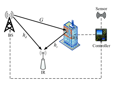
As shown in Fig. 1, we consider an IRS-based SR system consisting of a BS, an IRS, and an IR, where the BS transmits primary signals to the IR and the IRS delivers its own information to the IR by leveraging radio waves generated by the BS. We assume that the BS is equipped with $N$ transmit antennas, the IR is equipped with one antenna, and the IRS has $M$ reflecting elements. Let ${\bf{h}}_{d}\in{{\mathbb{C}}^{N\times 1}}$, ${\bf G}\in{{\mathbb{C}}^{M\times{N}}}$, and ${\bf h}_{r}\in{{\mathbb{C}}^{M\times 1}}$ denote the complex equivalent baseband channels between the BS and the IR, between the BS and the IRS, and between the IRS and the IR, respectively. The IRS reflection can be characterized by a diagonal reflection coefficient matrix ${{\bf{\Theta}}}{\rm{=diag}}\left({{e^{j{\theta_{1}}}},\ldots,{e^{j{\theta_{M}}}}}\right)$, where the reflection amplitude is fixed as $1$, and $\theta_{m}$ denotes the phase shift corresponding to the $m$th IRS reflecting element[4], [7],[33].

The CSR and PSR scenarios considered in this paper are described in the following.

II-A1 CSR scenario

In the CSR scenario, the symbol rate of the IRS transmission is much smaller than that of the primary transmission due to the limited computational and communication capabilities at the IRS. Denote the durations of the IRS symbol and the primary symbol by $T_{s}$ and $T_{x}$, respectively. Without loss of generality, we assume that each IRS symbol spans $L$ primary symbols, i.e., $T_{s}=LT_{x}$. Denote by $x[l]$, $0\leq l\leq L$, and $s$ the BS’s $l$th symbol and the IRS’s symbol, which is generated by the on/off state of the IRS, respectively. The $l$th symbol received by the IR is given by

$${y_{csr,r}}\left[l\right]=\underbrace{{\bf{h}}_{d}^{H}{\bf{w}}x\left[l\right]}_{{\rm{direct}}{\kern 1.0pt}{\kern 1.0pt}{\rm{link}}}+\underbrace{{\bf{h}}_{r}^{H}\left({s{\bf{\Theta}}}\right){\bf{Gw}}x\left[l\right]}_{{\rm{reflected}}{\kern 1.0pt}{\kern 1.0pt}{\rm{link}}}+{n_{r}[l]},$$ (1)

where ${\bf{w}}\in{{\mathbb{C}}^{N\times 1}}$ is the transmit beamforming vector at the BS, ${x[l]}\sim{\cal CN}\left({0,1}\right)$, and ${n_{r}[l]}\sim{\cal CN}\left({0,{\sigma^{2}}}\right)$ denotes the additive white Gaussian noise at the IR. We adopt the simple but widely used on-off keying (OOK) modulation for the information transmission of the IRS, i.e., $s=\left\{{0,1}\right\}$. We assume that the probability for the IRS to send symbol “1” is $\rho$, and that to send symbol “0” is $1-\rho$. Without loss of generality, we assume the IRS sends symbol “1” and symbol “0” with equal probability, i.e., $\rho=\frac{1}{2}$. We note that symbol “1”, i.e., $s=1$, implies the IRS is turned on and symbol “0”, i.e., $s=0$, implies the IRS is turned off.

The instantaneous achievable rate (bps/Hz) of the IRS-assisted primary system is given by

$${\tilde{R}_{csr,x}}\left(s\right)={\log_{2}}\left({1+\frac{{{{\left|{{\bf{h}}_{d}^{H}{\bf{w}}+{\bf{h}}_{r}^{H}\left({s{\bf{\Theta}}}\right){\bf{Gw}}}\right|}^{2}}}}{{{\sigma^{2}}}}}\right).$$ (2)

Since the instantaneous achievable rate ${\tilde{R}_{csr,x}}\left(s\right)$ depends on the IRS’s on/off state, the average achievable rate of the primary system is given by [28],[31]

$${R_{csr,x}} ={\mathbb{E}}_{s}\left\{{{{\tilde{R}}_{csr,x}}\left(s\right)}\right\}$$

$$=\left({1-\rho}\right){\log_{2}}\left({1+\frac{{{{\left|{{\bf{h}}_{d}^{H}{\bf{w}}}\right|}^{2}}}}{{{\sigma^{2}}}}}\right)+\rho{\log_{2}}\left({1+\frac{{{{\left|{{\bf{h}}_{d}^{H}{\bf{w}}+{{\bf{v}}^{H}}{\rm{diag}}\left({{\bf{h}}_{r}^{H}}\right){\bf{Gw}}}\right|}^{2}}}}{{{\sigma^{2}}}}}\right).$$ (3)

where ${{\bf{v}}^{H}}=\left({{e^{j{\theta_{1}}}},\ldots,{e^{j{\theta_{M}}}}}\right)$.

After successfully decoding the primary signal $x[l]$, the receiver can apply successive interference cancellation (SIC) to remove ${\bf{h}}_{d}^{H}{\bf{w}}x\left[l\right]$ from the received composite signal in (1). Thus, after removing this term, we obtain the intermediate IRS signal as follows

$${{\bar{y}}_{csr,r}}\left[l\right]={{\bf{v}}^{H}}{\rm{diag}}\left({{\bf{h}}_{r}^{H}}\right){\bf{Gw}}sx\left[l\right]+{n_{r}[l]},$$ (4)

Since each IRS symbol spans $L$ primary symbols for the CSR scenario, the IRS is affected by time-selective fading. By applying maximal-ratio-combining (MRC), the decision can be based on the following real sufficient statistic [34]

$${{\bar{y}}_{csr,r}} ={\mathop{\rm Re}\nolimits}\left\{{\sum\limits_{l=1}^{L}{{{\left({{{\bf{v}}^{H}}{\rm{diag}}\left({{\bf{h}}_{r}^{H}}\right){\bf{Gw}}x\left[l\right]}\right)}^{*}}{{\bar{y}}_{csr,r}}\left[l\right]}}\right\}$$

$$={\left|{{{\bf{v}}^{H}}{\rm{diag}}\left({{\bf{h}}_{r}^{H}}\right){\bf{Gw}}}\right|^{2}}\sum\limits_{l=1}^{L}{{{\left|{x\left[l\right]}\right|}^{2}}s}+{{\bar{n}}_{r}},$$ (5)

where ${{\bar{n}}_{r}}={\mathop{\rm Re}\nolimits}\left\{{{{\left({{{\bf{v}}^{H}}{\rm{diag}}\left({{\bf{h}}_{r}^{H}}\right){\bf{Gw}}}\right)}^{*}}\sum\limits_{l=1}^{L}{{x^{*}}\left[l\right]{n_{r}[l]}}}\right\}$. It is not difficult to see that

${{{\left({{{\bf{v}}^{H}}{\rm{diag}}\left({{\bf{h}}_{r}^{H}}\right){\bf{Gw}}}\right)}^{*}}\sum\limits_{l=1}^{L}{{x^{*}}\left[l\right]{n_{r}}[l]}}$ is still a CSCG random variable with the expectation and variance given by

$${\mathbb{E}}\left\{{{{\left({{{\bf{v}}^{H}}{\rm{diag}}\left({{\bf{h}}_{r}^{H}}\right){\bf{Gw}}}\right)}^{*}}\sum\limits_{l=1}^{L}{{x^{*}}\left[l\right]{n_{r}[l]}}}\right\}=0,$$

$${\mathop{{\mathbb{V}}{\rm ar}}}\left\{{{{\left({{{\bf{v}}^{H}}{\rm{diag}}\left({{\bf{h}}_{r}^{H}}\right){\bf{Gw}}}\right)}^{*}}\sum\limits_{l=1}^{L}{{x^{*}}\left[l\right]{n_{r}[l]}}}\right\}={{{\left|{{{\bf{v}}^{H}}{\rm{diag}}\left({{\bf{h}}_{r}^{H}}\right){\bf{Gw}}}\right|}^{2}}\sum\limits_{l=1}^{L}{{{\left|{x\left[l\right]}\right|}^{2}}}{\sigma^{2}}}.$$ (6)

As such, ${{\bar{n}}_{r}}$ is a real Gaussian random variable and it follows that

$${{\bar{n}}_{r}}\sim{\cal N}\left({0,{{\left|{{{\bf{v}}^{H}}{\rm{diag}}\left({{\bf{h}}_{r}^{H}}\right){\bf{Gw}}}\right|}^{2}}\sum\limits_{l=1}^{L}{{{\left|{x\left[l\right]}\right|}^{2}}}{\sigma^{2}}/2}\right).$$ (7)

We can rewrite (5) as follows

$${{\bar{y}}_{csr,r}}=\left\{\begin{array}[]{l}{\left|{{{\bf{v}}^{H}}{\rm{diag}}\left({{\bf{h}}_{r}^{H}}\right){\bf{Gw}}}\right|^{2}}\sum\limits_{l=1}^{L}{{{\left|{x\left[l\right]}\right|}^{2}}}+{{\bar{n}}_{r}},{\kern 1.0pt}{\kern 1.0pt}{\kern 1.0pt}s=1\\ {{\bar{n}}_{r}},{\kern 1.0pt}{\kern 1.0pt}{\kern 1.0pt}\qquad\qquad\qquad\qquad\qquad\qquad\quad~{}~{}s=0\end{array}\right.$$ (10)

Suppose that the hypotheses of sending symbol “1” and “0” are denoted by ${\cal H}_{1}$ and ${\cal H}_{0}$, respectively. Following [35], the BER for the IRS symbol assuming maximum likelihood (ML) detection can be expressed as

$${\bar{P}_{csr,e}} =\frac{1}{2}\Pr\left({{{\left|{{{\bf{v}}^{H}}{\rm{diag}}\left({{\bf{h}}_{r}^{H}}\right){\bf{Gw}}}\right|}^{2}}\sum\limits_{l=1}^{L}{{{\left|{x\left[l\right]}\right|}^{2}}}+{{\bar{n}}_{r}}<\bar{y}_{csr,r}^{th}|{{\cal H}_{1}}}\right)$$

$$+\frac{1}{2}\Pr\left({{{\bar{n}}_{r}}\geq\bar{y}_{csr,r}^{th}|{{\cal H}_{0}}}\right),$$ (11)

where $\bar{y}_{csr,r}^{th}={\left|{{{\bf{v}}^{H}}{\rm{diag}}\left({{\bf{h}}_{r}^{H}}\right){\bf{Gw}}}\right|^{2}}\sum\limits_{l=1}^{L}{{{\left|{x\left[l\right]}\right|}^{2}}}/2$. Define probability density function (PDF) ${f_{{{\bar{n}}_{r}}}}\left(t\right)=\frac{1}{{\sqrt{2\pi}{\sigma_{1}}}}\exp\left({-\frac{{{t^{2}}}}{{2\sigma_{1}^{2}}}}\right)$, where $\sigma_{1}^{2}={\left|{{{\bf{v}}^{H}}{\rm{diag}}\left({{\bf{h}}_{r}^{H}}\right){\bf{Gw}}}\right|^{2}}\sum\limits_{l=1}^{L}{{{\left|{x\left[l\right]}\right|}^{2}}{\sigma^{2}}}/2$. Then, the BER for CSR is obtained as

$${\bar{P}_{csr,e}} =\frac{1}{{\sqrt{2\pi}{\sigma_{1}}}}\int_{\bar{y}_{csr,r}^{th}}^{+\infty}{\exp\left({-\frac{{{t^{2}}}}{{2\sigma_{1}^{2}}}}\right)}dt$$

$$=Q\left({\frac{1}{{\sqrt{2}}}\left|{{{\bf{v}}^{H}}{\rm{diag}}\left({{\bf{h}}_{r}^{H}}\right){\bf{Gw}}}\right|\sqrt{\sum\nolimits_{l=1}^{L}{{{\left|{x\left[l\right]}\right|}^{2}}}}/\sigma}\right),$$ (12)

where $Q\left(x\right)=\frac{1}{{\sqrt{2\pi}}}\int_{x}^{\infty}{{e^{-\frac{{{t^{2}}}}{2}}}}dt$. Since $x[l]$ in (12) is a random variable, we are interested in the average BER for CSR. The primary signals are CSCG random variables and are independent identically distributed (i.i.d.), (12) is equivalent to the instantaneous BER for MRC combining of $L$ i.i.d. Rayleigh fading paths. Hence, according to [36], the closed-form expression for the average BER can be obtained as

$${P_{csr,e}}\overset{\triangle}{=}{\mathbb{E}}_{x[l]}\left\{{{{\bar{P}}_{csr,e}}}\right\}={\left({\frac{{1{\rm{-}}\mu}}{2}}\right)^{L}}\sum\limits_{l=0}^{L-1}{\left({\begin{array}[]{*{20}{c}}{L-1+l}\\ l\end{array}}\right)}{\left({\frac{{1+\mu}}{2}}\right)^{l}},$$ (15)

where $\mu=\sqrt{\frac{{{{\left|{{{\bf{v}}^{H}}{\rm{diag}}\left({{\bf{h}}_{r}^{H}}\right){\bf{Gw}}}\right|}^{2}}}}{{{{\left|{{{\bf{v}}^{H}}{\rm{diag}}\left({{\bf{h}}_{r}^{H}}\right){\bf{Gw}}}\right|}^{2}}+4{\sigma^{2}}}}}$ and $\left({\begin{array}[]{*{20}{c}}n\\ k\end{array}}\right)=\frac{{n\left({n-1}\right)\cdots\left({n-k+1}\right)}}{{k\left({k-1}\right)\cdots 1}}$.

II-A2 PSR scenario

Different from the CSR scenario, for PSR, the symbol rate of the IRS is equal to that of the primary transmission, i.e., $T_{s}=T_{x}$. Therefore, for PSR, the detection scheme for decoding the primary symbol and the IRS symbol is fundamentally different from that for CSR. Define by $s[l]$ the IRS’s $l$th transmit symbol. The $l$th received symbol at the IR is given by

$${y_{psr,r}}\left[l\right]=\underbrace{{\bf{h}}_{d}^{H}{\bf{w}}x\left[l\right]}_{{\rm{direct}}{\kern 1.0pt}{\kern 1.0pt}{\rm{link}}}+\underbrace{{\bf{h}}_{r}^{H}\left({s\left[l\right]{\bf{\Theta}}}\right){\bf{Gw}}x\left[l\right]}_{{\rm{reflected}}{\kern 1.0pt}{\kern 1.0pt}{\rm{link}}}+{n_{r}[l]}.$$ (16)

Similar to the CSR scenario, we first decode the primary symbol, i.e., $x[l]$, then subtract ${\bf{h}}_{d}^{H}{\bf{w}}x\left[l\right]$ from the combined signal, and finally extract the IRS symbol $s[l]$. Since $x[l]$ and $s[l]$ have the same symbol rate for PSR, the IRS treats the signal reflected from the IRS as interference with the average power given by ${\mathbb{E}}\left\{{{{\left|{{\bf{h}}_{r}^{H}\left({s\left[l\right]{\bf{\Theta}}}\right){\bf{Gw}}x\left[l\right]}\right|}^{2}}}\right\}=\rho{\left|{{{\bf{v}}^{H}}{\rm{diag}}\left({{\bf{h}}_{r}^{H}}\right){\bf{Gw}}}\right|^{2}}$ when decoding the primary signal $x[l]$. Therefore, the achievable rate for decoding the primary signal is given by

$${R_{psr,x}}={\log_{2}}\left({1+\frac{{{{\left|{{\bf{h}}_{d}^{H}{\bf{w}}}\right|}^{2}}}}{{\rho{{\left|{{{\bf{v}}^{H}}{\rm{diag}}\left({{\bf{h}}_{r}^{H}}\right){\bf{Gw}}}\right|}^{2}}{\rm{+}}{\sigma^{2}}}}}\right),$$ (17)

and then after removing ${\bf{h}}_{d}^{H}{\bf{w}}x\left[l\right]$ from (16), we have

$${\bar{y}_{psr,r}}\left[l\right]={\bf{h}}_{r}^{H}{\bf{\Theta Gw}}s\left[l\right]x\left[l\right]+{n_{r}[l]}.$$ (18)

Similar to the case of CSR, by setting $L=1$ in (15), the average BER for PSR can be expressed as

$${P_{psr,e}}=\frac{1}{2}{\rm{-}}\frac{1}{2}\sqrt{\frac{{{{\left|{{{\bf{v}}^{H}}{\rm{diag}}\left({{\bf{h}}_{r}^{H}}\right){\bf{Gw}}}\right|}^{2}}}}{{{{\left|{{{\bf{v}}^{H}}{\rm{diag}}\left({{\bf{h}}_{r}^{H}}\right){\bf{Gw}}}\right|}^{2}}+4{\sigma^{2}}}}}.$$ (19)

II-B Problem Formulation

II-B1 CSR scenario

Our goal is to minimize the BER of the IRS symbols by jointly optimizing the IRS phase shifts and the BS transmit beamformer while guaranteeing a minimum rate required for the primary network subject to the BS transmit power budget and the unit-modulus phase-shift constraints. Mathematically, the problem can be formulated as follows

$$\left({{\rm{P}}1}\right)\mathop{\min}\limits_{{\bf{w}},{\bf{v}}}{\left({\frac{{1{\rm{-}}\mu}}{2}}\right)^{L}}\sum\limits_{l=0}^{L-1}{\left({\begin{array}[]{*{20}{c}}{L-1+l}\\ l\end{array}}\right)}{\left({\frac{{1+\mu}}{2}}\right)^{l}}$$ (22)

$${\rm{s}}{\rm{.t}}{\rm{.}}~{}\left({1-\rho}\right){\log_{2}}\left({1+\frac{{{{\left|{{\bf{h}}_{d}^{H}{\bf{w}}}\right|}^{2}}}}{{{\sigma^{2}}}}}\right)+\rho{\log_{2}}\left({1+\frac{{{{\left|{{\bf{h}}_{d}^{H}{\bf{w}}+{{\bf{v}}^{H}}{\rm{diag}}\left({{\bf{h}}_{r}^{H}}\right){\bf{Gw}}}\right|}^{2}}}}{{{\sigma^{2}}}}}\right)\geq{R_{csr,{\rm th}}},$$ (23)

$$\qquad\left\|{\bf{w}}\right\|_{2}^{2}\leq{P_{\max}},$$ (24)

$$\qquad\left|{{{\bf{v}}_{m}}}\right|=1,\forall m,$$ (25)

where ${{{\bf{v}}_{m}}}$ denotes the $m$th element of ${\bf{v}}$, ${R_{csr,{\rm{th}}}}$ is the minimum rate required by the primary network for CSR, and ${P_{\max}}$ is the BS’s maximum transmit power. Problem $\left({{\rm{P}}1}\right)$ is non-convex and difficult to solve due to the highly coupled optimization variables in the objective function as well as constraints (23) and (25). There is no standard method for solving non-convex optimization problems optimally. As such, we propose a novel penalty-based algorithm to solve $\left({{\rm{P}}1}\right)$ to obtain a high-quality suboptimal solution in Section III.

II-B2 PSR scenario

Similarly, for PSR, we aim to jointly optimize the IRS phase shifts and the BS transmit beamformer to minimize the BER. Accordingly, the problem can be formulated as

$$\left({{\rm{P}}2}\right)\mathop{\min}\limits_{{\bf{w}},{\bf{v}}}\frac{1}{2}{\rm{-}}\frac{1}{2}\sqrt{\frac{{{{\left|{{{\bf{v}}^{H}}{\rm{diag}}\left({{\bf{h}}_{r}^{H}}\right){\bf{Gw}}}\right|}^{2}}}}{{{{\left|{{{\bf{v}}^{H}}{\rm{diag}}\left({{\bf{h}}_{r}^{H}}\right){\bf{Gw}}}\right|}^{2}}+4{\sigma^{2}}}}}$$

$${\rm{s}}{\rm{.t}}{\rm{.}}{\kern 1.0pt}{\kern 1.0pt}{\kern 1.0pt}{\kern 1.0pt}{\kern 1.0pt}{\kern 1.0pt}{\log_{2}}\left({1+\frac{{{{\left|{{\bf{h}}_{d}^{H}{\bf{w}}}\right|}^{2}}}}{{\rho{{\left|{{{\bf{v}}^{H}}{\rm{diag}}\left({{\bf{h}}_{r}^{H}}\right){\bf{Gw}}}\right|}^{2}}+{\sigma^{2}}}}}\right)\geq{R_{psr,{\rm{th}}}},$$ (26)

$$\qquad\eqref{csrP1const2},\eqref{csrP1const3},$$ (27)

where ${R_{psr,{\rm{th}}}}$ represents the minimum rate required for the primary network for PSR. Problem $\left({{\rm{P}}2}\right)$ is also challenging to solve for the following three reasons. First, the objective function of $\left({{\rm{P}}2}\right)$ is rather complicated, as it is non-convex due to the involvement of coupled optimization variables $\bf w$ and $\bf v$. Second, the optimization variables are intricately coupled in constraint (26). Third, constraint (25) is a unit-modulus constraint. Nevertheless, we propose an efficient bisection search based algorithm to solve problem $\left({{\rm{P}}2}\right)$ in Section IV.

III Penalty-based Algorithm for CSR Optimization Problem

In this section, we study the CSR scenario to minimize the BER of the IRS symbols and propose a novel penalty-based algorithm to solve $\left({{\rm{P}}1}\right)$, which involves a two-layer iteration, i.e., an inner layer iteration and an outer layer iteration. Specifically, the inner layer solves the penalized optimization problem, while the outer layer updates the penalty coefficient. We then alternately optimize the two layer iterations until convergence is achieved. Before proceeding to solving the problem, we observe that ${P_{csr,e}}$ given by (15) is monotonically decreasing in ${{{\left|{{{\bf{v}}^{H}}{\rm{diag}}\left({{\bf{h}}_{r}^{H}}\right){\bf{Gw}}}\right|^{2}}}}$, which implies that minimizing the BER $P_{csr,e}$ is equivalent to maximizing the SNR, i.e., $\frac{{{{\left|{{{\bf{v}}^{H}}{\rm{diag}}\left({{\bf{h}}_{r}^{H}}\right){\bf{Gw}}}\right|}^{2}}}}{{{\sigma^{2}}}}$. Thus, in the following, we adopt the SNR as the objective function to facilitate algorithm design.

III-A Problem Reformulation

We first introduce new auxiliary variables ${{\mu_{1}}}$ and ${{\mu_{2}}}$ satisfying ${\mu_{1}}{\rm{=}}\frac{{{{\bf{v}}^{H}}{\rm{diag}}\left({{\bf{h}}_{r}^{H}}\right){\bf{Gw}}}}{\sigma}$ and ${\mu_{2}}=\frac{{{\bf{h}}_{d}^{H}{\bf{w}}}}{\sigma}$. Then, problem $\left({{\rm{P}}1}\right)$ is equivalent to

$$\left({{\rm{\bar{P}}}1}\right) \mathop{\max}\limits_{{\bf{w}},{\bf{v}},{\mu_{1}},{\mu_{2}}}{\left|{{\mu_{1}}}\right|^{2}}$$

$${\rm{s}}{\rm{.t}}{\rm{.}}{\kern 1.0pt}{\kern 1.0pt}{\kern 1.0pt}{\kern 1.0pt}{\kern 1.0pt}{\kern 1.0pt}\left({1-\rho}\right){\log_{2}}\left({1+{{\left|{{\mu_{2}}}\right|}^{2}}}\right)+\rho{\log_{2}}\left({1+{{\left|{{\mu_{1}}+{\mu_{2}}}\right|}^{2}}}\right)\geq{R_{csr,{\rm{th}}}},$$ (28)

$$\qquad{\mu_{1}}{\rm{=}}\frac{{{{\bf{v}}^{H}}{\rm{diag}}\left({{\bf{h}}_{r}^{H}}\right){\bf{Gw}}}}{\sigma},$$ (29)

$$\qquad{\mu_{2}}=\frac{{{\bf{h}}_{d}^{H}{\bf{w}}}}{\sigma},$$ (30)

$$\qquad\eqref{csrP1const2},\eqref{csrP1const3}.$$ (31)

We then use (29) and (30) as penalty terms that are added to the objective function of $\left({{\rm{\bar{P}}}1}\right)$, yielding the following optimization problem

$$\left({{\rm{\bar{P}}}1{\rm{-}}1}\right) \mathop{\max}\limits_{{\bf{w}},{\bf{v}},{\mu_{1}},{\mu_{2}}}{\left|{{\mu_{1}}}\right|^{2}}-\frac{1}{{2\eta}}\left({{{\left|{{\mu_{1}}-\frac{{{{\bf{v}}^{H}}{\rm{diag}}\left({{\bf{h}}_{r}^{H}}\right){\bf{Gw}}}}{\sigma}}\right|}^{2}}+{{\left|{{\mu_{2}}-\frac{{{\bf{h}}_{d}^{H}{\bf{w}}}}{\sigma}}\right|}^{2}}}\right)$$ (32)

$${\rm{s}}{\rm{.t}}{\rm{.}}{\kern 1.0pt}{\kern 1.0pt}{\kern 1.0pt}{\kern 1.0pt}{\kern 1.0pt}{\kern 1.0pt}\eqref{csrP1const2},\eqref{csrP1const3},\eqref{csrbarP1const1},$$ (33)

where $\eta$ ($\eta>0$) is a penalty coefficient that penalizes the violation of equality constraints (29) and (30). By gradually decreasing the value of $\eta$ in the outer layer until it approaches zero, it follows that $\frac{1}{{2\eta}}\to\infty$. As such, the penalty terms will be forced to zero eventually, i.e., $\left|{{\mu_{1}}-\frac{{{{\bf{v}}^{H}}{\rm{diag}}\left({{\bf{h}}_{r}^{H}}\right){\bf{Gw}}}}{\sigma}}\right|=0$ and $\left|{{\mu_{2}}-\frac{{{\bf{h}}_{d}^{H}{\bf{w}}}}{\sigma}}\right|=0$, which indicates that the newly added equality constraints (29) and (30) will be satisfied after convergence. However, for a given $\eta$, $\left({{\rm{\bar{P}}}1{\rm{-}}1}\right)$ is still a non-convex optimization problem due to the coupled optimization variables in both the objective function and constraint (28), and the unit-modulus constraint in (25). To address this difficulty, we first divide the variables into three blocks, namely, 1) auxiliary variables $\{\mu_{1},\mu_{2}\}$, 2) BS transmit beamformer $\bf w$, and 3) phase shift vector $\bf v$, and alternately optimize each block with the other two blocks of variables fixed until convergence is achieved.

III-B Inner Layer Iteration

1) Optimizing auxiliary variables $\{\mu_{1},\mu_{2}\}$ for the given BS transmit beamformer $\bf w$ and phase shift vector $\bf v$. This subproblem is formulated as

$$\left({{\rm{\bar{P}}}1{\rm{-2}}}\right) \mathop{\max}\limits_{{\mu_{1}},{\mu_{2}}}~{}{\left|{{\mu_{1}}}\right|^{2}}-\frac{1}{{2\eta}}\left({{{\left|{{\mu_{1}}-\frac{{{{\bf{v}}^{H}}{\rm{diag}}\left({{\bf{h}}_{r}^{H}}\right){\bf{Gw}}}}{\sigma}}\right|}^{2}}+{{\left|{{\mu_{2}}-\frac{{{\bf{h}}_{d}^{H}{\bf{w}}}}{\sigma}}\right|}^{2}}}\right)$$

$${\rm{s}}{\rm{.t}}{\rm{.}}{\kern 1.0pt}{\kern 1.0pt}{\kern 1.0pt}{\kern 1.0pt}{\kern 1.0pt}{\kern 1.0pt}\eqref{csrbarP1const1}.$$ (34)

Note that $\left({{\rm{\bar{P}}}1{\rm{-2}}}\right)$ is neither concave nor quasi-concave due to the non-convex constraint (28). In addition, we must have $1{\rm{-}}\frac{1}{{2\eta}}\leq 0$ in the objective function, i.e., $\eta\leq\frac{1}{2}$, since otherwise we can increase $\mu_{1}$ to obtain an infinite value of the objective function. As such, the objective function of $\left({{\rm{\bar{P}}}1{\rm{-2}}}\right)$ is jointly convex w.r.t. $\mu_{1}$ and $\mu_{2}$. In the following, we propose to leverage the successive convex approximation (SCA) technique to solve $\left({{\rm{\bar{P}}}1{\rm{-2}}}\right)$. Recall that any convex function is globally lower-bounded by its first-order Taylor expansion at any feasible point. Therefore, for any given points $\mu^{r}_{1}$ and $\mu^{r}_{2}$ at the $r$th iteration, we have

$${\left|{{\mu_{2}}}\right|^{2}}\geq{-{{\left|{\mu_{2}^{r}}\right|}^{2}}+2{\rm{Re}}\left\{{\mu_{2}^{H}\mu_{2}^{r}}\right\}},$$ (35)

$${\left|{{\mu_{1}}{\rm{+}}{\mu_{2}}}\right|^{2}}\geq{-{{\left|{\mu_{1}^{r}+\mu_{2}^{r}}\right|}^{2}}+2{\rm{Re}}\left\{{{{\left({{\mu_{1}}+{\mu_{2}}}\right)}^{H}}\left({\mu_{1}^{r}+\mu_{2}^{r}}\right)}\right\}}.$$ (36)

As a result, for any given points $\mu^{r}_{1}$ and $\mu^{r}_{2}$, we obtain the following optimization problem

$$\left({{\rm{\bar{P}}}1{\rm{-3}}}\right) \mathop{\max}\limits_{{\mu_{1}},{\mu_{2}}}~{}{\left|{{\mu_{1}}}\right|^{2}}-\frac{1}{{2\eta}}\left({{{\left|{{\mu_{1}}-\frac{{{{\bf{v}}^{H}}{\rm{diag}}\left({{\bf{h}}_{r}^{H}}\right){\bf{Gw}}}}{\sigma}}\right|}^{2}}+{{\left|{{\mu_{2}}-\frac{{{\bf{h}}_{d}^{H}{\bf{w}}}}{\sigma}}\right|}^{2}}}\right)$$

$${\rm{s}}{\rm{.t}}{\rm{.}}{\kern 1.0pt}{\kern 1.0pt}{\kern 1.0pt}{\kern 1.0pt}{\kern 1.0pt}{\kern 1.0pt}\left({1-\rho}\right){\log_{2}}\left({1-{{\left|{\mu_{2}^{r}}\right|}^{2}}+2{\rm{Re}}\left\{{\mu_{2}^{H}\mu_{2}^{r}}\right\}}\right)+$$

$$\qquad\rho{\log_{2}}\left({1-{{\left|{\mu_{1}^{r}+\mu_{2}^{r}}\right|}^{2}}+2{\rm{Re}}\left\{{{{\left({{\mu_{1}}+{\mu_{2}}}\right)}^{H}}\left({\mu_{1}^{r}+\mu_{2}^{r}}\right)}\right\}}\right)\geq{R_{csr,{\rm{th}}}}.$$ (37)

It can be readily verified that the objective function of $\left({{\rm{\bar{P}}}1{\rm{-3}}}\right)$ and new constraint (37) are convex. Thus, $\left({{\rm{\bar{P}}}1{\rm{-3}}}\right)$ can be efficiently solved by using standard convex optimization techniques [37]. It is worth pointing out that the obtained objective value of $\left({{\rm{\bar{P}}}1{\rm{-3}}}\right)$ serves as a lower-bound for $\left({{\rm{\bar{P}}}1{\rm{-2}}}\right)$ due to the Taylor expansion approximation in (35) and (36).

2) Optimizing BS transmit beamformer $\bf w$ for the given phase shift $\bf v$ and auxiliary variables $\{\mu_{1},\mu_{2}\}$. This subproblem can be expressed as

$$\left({{\rm{\bar{P}}}1{\rm{-4}}}\right) \mathop{\min}\limits_{\bf{w}}{\left|{{\mu_{1}}-\frac{{{{\bf{v}}^{H}}{\rm{diag}}\left({{\bf{h}}_{r}^{H}}\right){\bf{Gw}}}}{\sigma}}\right|^{2}}+{\left|{{\mu_{2}}-\frac{{{\bf{h}}_{d}^{H}{\bf{w}}}}{\sigma}}\right|^{2}}$$

$${\rm{s}}{\rm{.t}}{\rm{.}}{\kern 1.0pt}{\kern 1.0pt}{\kern 1.0pt}{\kern 1.0pt}{\kern 1.0pt}{\kern 1.0pt}\eqref{csrP1const2}.$$ (38)

It can be readily observed that $\left({{\rm{\bar{P}}}1{\rm{-4}}}\right)$ is a convex quadratically constrained quadratic program (QCQP), which can be solved by the interior point method [37]. However, the complexity of solving $\left({{\rm{\bar{P}}}1{\rm{-4}}}\right)$ by the interior point method is ${\cal O}{\left(N^{3.5}\right)}$, which is rather high especially when the number of antennas $N$ is large. To reduce the computational complexity, we obtain a semi-closed-form yet optimal solution for the BS transmit beamformer $\bf w$ by using the Lagrange duality method [37]. Specifically, by introducing dual variable $\lambda$ ($\lambda\geq 0$) associated with constraint (24), the Lagrangian function of $\left({{\rm{\bar{P}}}1{\rm{-4}}}\right)$ is given by

$${\cal L}\left({{\bf{w}},\lambda}\right)={\left|{{\mu_{1}}-\frac{{{{\bf{v}}^{H}}{\rm{diag}}\left({{\bf{h}}_{r}^{H}}\right){\bf{Gw}}}}{\sigma}}\right|^{2}}+{\left|{{\mu_{2}}-\frac{{{\bf{h}}_{d}^{H}{\bf{w}}}}{\sigma}}\right|^{2}}+\lambda\left({\left\|{\bf{w}}\right\|_{2}^{2}-{P_{\max}}}\right).$$ (39)

By taking the first-order derivative of ${\cal L}\left({{\bf{w}},\lambda}\right)$ w.r.t. $\bf w$ and setting it to zero, we obtain the optimal solution as

$${\bf{w}}\left(\lambda\right){\rm{=}}{\left({\frac{{{{\bf{G}}^{H}}{\rm{diag}}\left({{{\bf{h}}_{r}}}\right){\bf{v}}{{\bf{v}}^{H}}{\rm{diag}}\left({{\bf{h}}_{r}^{H}}\right){\bf{G}}{\rm{+}}{{\bf{h}}_{d}}{\bf{h}}_{d}^{H}}}{{{\sigma^{2}}}}{\rm{+}}\lambda{{\bf{I}}_{N}}}\right)^{\dagger}}\left({\frac{{{\mu_{1}}{{\bf{G}}^{H}}{\rm{diag}}\left({{{\bf{h}}_{r}}}\right){\bf{v}}{\rm{+}}{\mu_{2}}{{\bf{h}}_{d}}}}{\sigma}}\right).$$ (40)

Recall that for the optimal solution ${{\bf{w}}^{{\rm{opt}}}}\left({{\lambda^{{\rm{opt}}}}}\right)$ and ${\lambda^{{\rm{opt}}}}$, the following complementary slackness condition must be satisfied[37]

$${\lambda^{{\rm{opt}}}}\left({{{\left\|{{{\bf{w}}^{{\rm{opt}}}}\left({{\lambda^{{\rm{opt}}}}}\right)}\right\|}^{2}}-{P_{\max}}}\right)=0.$$ (41)

We first check whether ${\lambda^{{\rm{opt}}}}=0$ is the optimal solution or not. If

$${\left\|{{{\bf{w}}^{{\rm{opt}}}}\left(0\right)}\right\|^{2}}-{P_{\max}}<0,$$ (42)

which indicates that the optimal dual variable $\lambda$ equals $0$, the optimal BS beamformer is given by ${{\bf{w}}^{{\rm{opt}}}}\left(0\right){\rm{=}}{\left({{{{{\bf{G}}^{H}}{\rm{diag}}\left({{{\bf{h}}_{r}}}\right){\bf{v}}{{\bf{v}}^{H}}{\rm{diag}}\left({{\bf{h}}_{r}^{H}}\right){\bf{G}}{\rm{+}}{{\bf{h}}_{d}}{\bf{h}}_{d}^{H}}\mathord{\left/{\vphantom{{{{\bf{G}}^{H}}{\rm{diag}}\left({{{\bf{h}}_{r}}}\right){\bf{v}}{{\bf{v}}^{H}}{\rm{diag}}\left({{\bf{h}}_{r}^{H}}\right){\bf{G}}{\rm{+}}{{\bf{h}}_{d}}{\bf{h}}_{d}^{H}}{{\sigma^{2}}}}}\right.\kern-1.2pt}{{\sigma^{2}}}}}\right)^{{\dagger}}}\left({\frac{{{\mu_{1}}{{\bf{G}}^{H}}{\rm{diag}}\left({{{\bf{h}}_{r}}}\right){\bf{v}}{\rm{+}}{\mu_{2}}{{\bf{h}}_{d}}}}{\sigma}}\right)$, otherwise, the optimal $\lambda$ is a positive value, which can be calculated as follows.

Defining ${\bf{S}}={{\bf{G}}^{H}}{\rm{diag}}\left({{{\bf{h}}_{r}}}\right){\bf{v}}{{\bf{v}}^{H}}{\rm{diag}}\left({{\bf{h}}_{r}^{H}}\right){\bf{G}}{\rm{+}}{{\bf{h}}_{d}}{\bf{h}}_{d}^{H}/{\sigma^{2}}$ and ${\bf{z}}={\mu_{1}}{{\bf{G}}^{H}}{\rm{diag}}\left({{{\bf{h}}_{r}}}\right){\bf{v}}{\rm{+}}{\mu_{2}}{{\bf{h}}_{d}}/\sigma$, we have

$$\left\|{{\bf{w}}\left(\lambda\right)}\right\|_{2}^{2}{\rm{=tr}}\left({{{\left({{\bf{S}}{\rm{+}}\lambda{{\bf{I}}_{N}}}\right)}^{-2}}{\bf{z}}{{\bf{z}}^{H}}}\right).$$ (43)

It can be readily shown that ${\bf{S}}$ is a positive semi-definite matrix. We thus have ${\bf{S}}{\rm{=}}{\bf{U\Sigma}}{{\bf{U}}^{H}}$ by performing eigenvalue decomposition. Substituting ${\bf{S}}{\rm{=}}{\bf{U\Sigma}}{{\bf{U}}^{H}}$ into (43), we arrive at

$$\left\|{{\bf{w}}\left(\lambda\right)}\right\|_{2}^{2} {\rm{=tr}}\left({{{\left({{\bf{\Sigma}}{\rm{+}}\lambda{{\bf{I}}_{N}}}\right)}^{-2}}{{\bf{U}}^{H}}{\bf{z}}{{\bf{z}}^{H}}{\bf{U}}}\right)$$

$${\rm{=}}\sum\limits_{i=1}^{{s_{r}}}{\frac{{{{\left({{{\bf{U}}^{H}}{\bf{z}}{{\bf{z}}^{H}}{\bf{U}}}\right)}_{i,i}}}}{{{{\left({{{\bf{\Sigma}}_{i,i}}+\lambda}\right)}^{2}}}}}+\sum\limits_{i={s_{r}}+1}^{N}{\frac{{{{\left({{{\bf{U}}^{H}}{\bf{z}}{{\bf{z}}^{H}}{\bf{U}}}\right)}_{i,i}}}}{{{\lambda^{2}}}}},$$ (44)

where $s_{r}$ denotes the number of non-zero eigenvalues of ${\bf{S}}$. Note that since each main diagonal element of ${{{\bf{U}}^{H}}{\bf{z}}{{\bf{z}}^{H}}{\bf{U}}}$ is non-negative, $\left\|{{\bf{w}}\left(\lambda\right)}\right\|_{2}^{2}$ is monotonically decreasing w.r.t. dual variable $\lambda$. Therefore, the optimal ${{\lambda^{{\rm{opt}}}}}$ can be obtained by using the bisection search method to find the solution that satisfies the following equation

$$\sum\limits_{i=1}^{{s_{r}}}{\frac{{{{\left({{{\bf{U}}^{H}}{\bf{z}}{{\bf{z}}^{H}}{\bf{U}}}\right)}_{i,i}}}}{{{{\left({{{\bf{\Sigma}}_{i,i}}+{\lambda^{{\rm{opt}}}}}\right)}^{2}}}}}+\sum\limits_{i={s_{r}}+1}^{N}{\frac{{{{\left({{{\bf{U}}^{H}}{\bf{z}}{{\bf{z}}^{H}}{\bf{U}}}\right)}_{i,i}}}}{{{{\left({{\lambda^{{\rm{opt}}}}}\right)}^{2}}}}}={P_{\max}}.$$ (45)

Then, substituting the optimal ${{\lambda^{{\rm{opt}}}}}$ into (40), we obtain the optimal BS beamformer vector ${{\bf{w}}^{{\rm{opt}}}}\left({{\lambda^{{\rm{opt}}}}}\right)$. Note that for the bisection search, the low bound of $\lambda$, denoted by $\lambda^{\rm lb}$, can be set as a sufficiently small non-negative value, while the upper bound of $\lambda$, denoted by $\lambda^{\rm up}$, can be calculated as ${\lambda^{{\rm{up}}}}=\sqrt{\sum\limits_{i=1}^{N}{{{\left({{{\bf{U}}^{H}}{\bf{z}}{{\bf{z}}^{H}}{\bf{U}}}\right)}_{i,i}}}/{P_{\max}}}$. The detailed procedure for solving $\left({{\rm{\bar{P}}}1{\rm{-4}}}\right)$ is summarized in Algorithm 1. Note that the complexity of Algorithm 1 is ${\cal O}\left({\log_{2}\left({\frac{{{\lambda^{{\rm{up}}}}-{\lambda^{{\rm{lb}}}}}}{\varepsilon}}\right)}N^{3}\right)$, which is much lower than that of the interior point method.

Algorithm 1 Proposed Lagrange duality method for solving problem $\left({{\rm{\bar{P}}}1{\rm{-4}}}\right)$.

1:  Initialize ${\lambda^{{\rm{lb}}}}$, ${\lambda^{{\rm{up}}}}$, and $\varepsilon$.

2:  If $\left\|{{\bf{w}}\left(0\right)}\right\|_{2}^{2}\leq{P_{\max}}$, the optimal BS beamforming vector is given by ${{{\bf{w}}^{{\rm{opt}}}}\left(0\right)}$, and then terminate the algorithm; otherwise, go to step $3$.

3:  Repeat

4:   Compute $\lambda=\frac{{{\lambda^{{\rm{lb}}}}+{\lambda^{{\rm{up}}}}}}{2}$.

5:   If $\left\|{{\bf{w}}\left(\lambda\right)}\right\|_{2}^{2}\leq{P_{\max}}$, let ${\lambda^{{\rm{up}}}}=\lambda$, otherwise, let ${\lambda^{{\rm{lb}}}}=\lambda$.

6:  Until $\left|{{\lambda^{{\rm{up}}}}-{\lambda^{{\rm{lb}}}}}\right|\leq\varepsilon$.

7:  Output: Optimal BS beamformer ${{\bf{w}}^{{\rm{opt}}}}\left({{\lambda^{{\rm{lb}}}}}\right)$.

3) Optimizing phase shift vector $\bf v$ for given BS transmit beamformer $\bf w$ and auxiliary variables $\{\mu_{1},\mu_{2}\}$. This subproblem is given by

$$\left({{\rm{\bar{P}}}1{\rm{-5}}}\right) \mathop{\min}\limits_{\bf{v}}{\left|{{\mu_{1}}-\frac{{{{\bf{v}}^{H}}{\rm{diag}}\left({{\bf{h}}_{r}^{H}}\right){\bf{Gw}}}}{\sigma}}\right|^{2}}$$

$${\rm{s}}{\rm{.t}}{\rm{.}}{\kern 1.0pt}{\kern 1.0pt}{\kern 1.0pt}{\kern 1.0pt}{\kern 1.0pt}{\kern 1.0pt}\eqref{csrP1const3}.$$ (46)

Although the objective function of $\left({{\rm{\bar{P}}}1{\rm{-5}}}\right)$ is a quadratic function, the unit-modulus constraints in (25) are still non-convex. In the following, we obtain a locally optimal closed-form solution for $\bf v$ by leveraging the Majorization-Minimization (MM) method[38, 39]. The key idea of using the MM method lies in constructing a convex surrogate function that is an upper bound of the objective function of $\left({{\rm{\bar{P}}}1{\rm{-5}}}\right)$. Define $f\left({\bf{v}}\right)$ as the objective function and ${{{\bf{v}}^{r}}}$ as the initial point for ${\bf{v}}$ at the $r$th iteration, the surrogate function, denoted by $\hat{f}\left({{\bf{v}}{\rm{|}}{{\bf{v}}^{r}}}\right)$, should satisfy with the following three conditions: 1) $\hat{f}\left({{\bf{v}}{\rm{|}}{{\bf{v}}^{r}}}\right)\geq f\left({\bf{v}}\right)$; 2) $\hat{f}\left({{{\bf{v}}^{r}}{\rm{|}}{{\bf{v}}^{r}}}\right)=f\left({{{\bf{v}}^{r}}}\right)$; 3) ${\nabla_{{{\bf{v}}^{r}}}}\hat{f}\left({{{\bf{v}}^{r}}{\rm{|}}{{\bf{v}}^{r}}}\right)={\nabla_{{{\bf{v}}^{r}}}}f\left({{{\bf{v}}^{r}}}\right)$, where 1) means that $\hat{f}\left({{\bf{v}}{\rm{|}}{{\bf{v}}^{r}}}\right)$ serves an upper bound function of $f\left({\bf{v}}\right)$, 2) implies that $\hat{f}\left({{\bf{v}}{\rm{|}}{{\bf{v}}^{r}}}\right)$ and $f\left({\bf{v}}\right)$ have the same function value at point ${{{\bf{v}}^{r}}}$, and 3) indicates $\hat{f}\left({{\bf{v}}{\rm{|}}{{\bf{v}}^{r}}}\right)$ and $f\left({\bf{v}}\right)$ have the same gradient at point ${{{\bf{v}}^{r}}}$. As a result, we have the following lemma:

Lemma 1: Based on [38], at the initial point ${{{\bf{v}}^{r}}}$, a surrogate function $\hat{f}\left({{\bf{v}}{\rm{|}}{{\bf{v}}^{r}}}\right)$ for quadratic function $f({\bf v})={{\bf{v}}^{H}}{\bf{Av}}$ is given by

$$\hat{f}\left({{\bf{v}}|{{\bf{v}}^{r}}}\right)={\lambda_{\max}}{{\bf{v}}^{H}}{\bf{v}}-2{\mathop{\rm Re}\nolimits}\left\{{{{\bf{v}}^{H}}\left({{\lambda_{\max}}{{\bf{I}}_{M}}-{\bf{A}}}\right){{\bf{v}}^{r}}}\right\}+{{\bf{v}}^{r,H}}\left({{\lambda_{\max}}{{\bf{I}}_{M}}-{\bf{A}}}\right){{\bf{v}}^{r}},$$ (47)

where ${\bf{A}}=\frac{{{\rm{diag}}\left({{\bf{h}}_{r}^{H}}\right){\bf{Gw}}{{\bf{w}}^{H}}{{\bf{G}}^{H}}{\rm{diag}}\left({{{\bf{h}}_{r}}}\right)}}{{{\sigma^{2}}}}$, and ${\lambda_{\max}}$ represents the maximum eigenvalue of ${\bf{A}}$.

Substituting $\hat{f}\left({{\bf{v}}|{{\bf{v}}^{r}}}\right)$ for $f\left({\bf{v}}\right)$ and plugging it into the objective function of $\left({{\rm{\bar{P}}}1{\rm{-5}}}\right)$ as well as ignoring the irrelevant constants w.r.t. $\bf v$, the phase shift $\bf v$ can be obtained by solving the following problem

$$\left({{\rm{\bar{P}}}1{\rm{-6}}}\right) \mathop{\max}\limits_{\bf{v}}~{}{\mathop{\rm Re}\nolimits}\left\{{{{\bf{v}}^{H}}{{\bf{q}}^{r}}}\right\}$$

$${\rm{s}}{\rm{.t}}{\rm{.}}{\kern 1.0pt}{\kern 1.0pt}{\kern 1.0pt}{\kern 1.0pt}{\kern 1.0pt}{\kern 1.0pt}\eqref{csrP1const3},$$ (48)

where ${{\bf{q}}^{r}}=\left({{\lambda_{\max}}{{\bf{I}}_{M}}-{\bf{A}}}\right){{\bf{v}}^{r}}+\frac{{{\rm{diag}}\left({{\bf{h}}_{r}^{H}}\right){\bf{Gw}}\mu_{1}^{H}}}{\sigma}$. Obviously, the optimal phase shift vector for $\left({{\rm{\bar{P}}}1{\rm{-6}}}\right)$ is given by ${{\bf{v}}^{{\rm{opt}}}}=\exp\left({j\arg\left({{{\bf{q}}^{r}}}\right)}\right)$. Note that the obtained optimal solution ${{\bf{v}}^{{\rm{opt}}}}$ for $\left({{\rm{\bar{P}}}1{\rm{-6}}}\right)$ is guaranteed to be a locally optimal solution for the original problem $\left({{\rm{\bar{P}}}1{\rm{-5}}}\right)$ [38, 39].

III-C Outer Layer Iteration

In the outer layer, we gradually decrease the value of penalty coefficient $\eta^{r}$ in the $r$th iteration by updating it as follows

$$\eta^{r}=c\eta^{r-1},$$ (49)

where $c$ $(0<c<1)$ is a scaling factor. Here, a larger value of $c$ can achieve better performance but at the cost of more iterations required in the outer layer.

III-D Overall Algorithm

The constraint violation of the proposed penalty-based algorithm is qualified by

$$\xi{\rm{=}}\max\left\{{\left|{{\mu_{1}}-\frac{{{{\bf{v}}^{H}}{\rm{diag}}\left({{\bf{h}}_{r}^{H}}\right){\bf{Gw}}}}{\sigma}}\right|,\left|{{\mu_{2}}-\frac{{{\bf{h}}_{d}^{H}{\bf{w}}}}{\sigma}}\right|}\right\}.$$ (50)

The proposed penalty-based algorithm is summarized in Algorithm 2.

Algorithm 2 Proposed penalty-based algorithm for solving problem $\left({{\rm{\bar{P}}}1-1}\right)$.

1:  Initialize phase shift vector ${\bf v}^{r_{1}}$, auxiliary variables $\{\mu_{1}^{r_{1}},\mu_{2}^{r_{1}}\}$, penalty coefficient $\eta^{r_{2}}$, scaling factor $c$, predefined thresholds $\varepsilon_{1}$ and $\varepsilon_{2}$, inner layer iteration index $r_{1}=0$, outer layer iteration index $r_{2}=0$.

2:  Repeat: outer layer

3:   Repeat: inner layer

4:    Update auxiliary variables, denoted by $\{\mu_{1}^{r_{1}+1},\mu_{2}^{r+1}\}$, by solving problem $\left({{\rm{\bar{P}}}1{\rm{-3}}}\right)$.

5:    Update BS transmit beamformer, denoted by ${\bf w}^{r_{1}+1}$, by solving problem $\left({{\rm{\bar{P}}}1{\rm{-4}}}\right)$.

6:    Update phase shift vector, denoted by ${\bf v}^{r_{1}+1}$, by solving problem $\left({{\rm{\bar{P}}}1{\rm{-6}}}\right)$.

7:    Set $r_{1}=r_{1}+1$.

8:   Until the fractional increase of the objective value of $\left({{\rm{\bar{P}}}1{\rm{-1}}}\right)$ is below $\varepsilon_{1}$.

9:   Update the penalty coefficient, denoted by $\eta^{r_{2}+1}$, based on (49).

10:   Set $r_{2}=r_{2}+1$ and $r_{1}=0$.

11:  Until constraint violation indicator $\xi$ in (50) is smaller than $\varepsilon_{2}$.

Lemma 2: The obtained solution $\{{\bf w},{\bf v},\mu_{1},\mu_{2}\}$ converges to a point fulfilling the Karush–Kuhn –Tucker (KKT) optimality conditions of original problem $\left({{\rm{\bar{P}}}1}\right)$.

Proof: Note that with the proper variable partitioning in our proposed algorithm, there is no constraint coupling between the variables in different blocks, as seen from $\left({{\rm{\bar{P}}}1{\rm{-}}3}\right)$, $\left({{\rm{\bar{P}}}1{\rm{-}}4}\right)$, and $\left({{\rm{\bar{P}}}1{\rm{-}}6}\right)$. In addition, in step $4$ of Algorithm 2, $\left({{\rm{\bar{P}}}1{\rm{-}}3}\right)$ is solved by an SCA method and a locally optimal solution is obtained. In step $5$, a globally optimal solution is obtained by using the Lagrange duality method for $\left({{\rm{\bar{P}}}1{\rm{-}}4}\right)$. In step $6$, a locally optimal solution is obtained by using the MM method to solve $\left({{\rm{\bar{P}}}1{\rm{-}}6}\right)$. Following Theorem 4.1 in [40] together with the fact that for each subproblem in the inner layer at least a locally optimal solution is obtained, the proposed algorithm is guaranteed to find a locally optimal solution of $\left({{\rm{\bar{P}}}1}\right)$.

IV Bisection Search-based Algorithm for PSR Optimization Problem

In this section, we study the PSR scenario and minimize the BER of the IRS symbols. It can be readily seen that the objective function of $\left({{\rm{P}}2}\right)$ is a monotonically decreasing function in ${\left|{{{\bf{v}}^{H}}{\rm{diag}}\left({{\bf{h}}_{r}^{H}}\right){\bf{Gw}}}\right|^{2}}$. Thus, we can equivalently maximize the corresponding SNR instead. The problem can be recast as follows

$$\left({{\rm{\bar{P}}}2}\right) \mathop{\max}\limits_{{\bf{w}},{\bf{v}},\beta}~{}\beta$$

$${\rm s.t.}~{}\frac{{{{\left|{{{\bf{v}}^{H}}{\rm{diag}}\left({{\bf{h}}_{r}^{H}}\right){\bf{Gw}}}\right|}^{2}}}}{{{\sigma^{2}}}}\geq\beta,$$ (51)

$$\qquad\eqref{csrP1const2},\eqref{csrP1const3},\eqref{psrP2const1}.$$ (52)

In the following, we propose an efficient bisection search based algorithm to solve $\left({{\rm{\bar{P}}}2}\right)$. However, the search range for $\beta$ is in principle infinite, which would make the proposed algorithm inefficient. To tackle this issue, we first confine the search space by deriving an upper bound for $\beta$.

IV-A Confined Search Range

Problem $\left({{\rm{\bar{P}}}2}\right)$ can be solved by finding the maximum value of $\beta$ that satisfies all the constraints. Based on (24) and (51), we have the following inequality

$$\beta\leq\frac{{{{\left|{{{\bf{v}}^{H}}{\rm{diag}}\left({{\bf{h}}_{r}^{H}}\right){\bf{Gw}}}\right|}^{2}}}}{{{\sigma^{2}}}}\overset{(a)}{\leq}\frac{{{P_{\max}}{{\left\|{{{\bf{v}}^{H}}{\rm{diag}}\left({{\bf{h}}_{r}^{H}}\right){\bf{G}}}\right\|}^{2}}}}{{{\sigma^{2}}}},$$ (53)

where $(a)$ holds since the optimal beamforming vector $\bf w$ that maximizes ${{{\left|{{{\bf{v}}^{H}}{\rm{diag}}\left({{\bf{h}}_{r}^{H}}\right){\bf{Gw}}}\right|}^{2}}}$ is ${\bf{w}}=\frac{{\sqrt{{P_{\max}}}{{\bf{G}}^{H}}{\rm{diag}}\left({{{\bf{h}}_{r}}}\right){\bf{v}}}}{{\left\|{{{\bf{G}}^{H}}{\rm{diag}}\left({{{\bf{h}}_{r}}}\right){\bf{v}}}\right\|}}$. Similar to Lemma 1, a surrogate function for $\frac{{{{\bf{v}}^{H}}{\rm{diag}}\left({{\bf{h}}_{r}^{H}}\right){\bf{G}}{{\bf{G}}^{H}}{\rm{diag}}\left({{{\bf{h}}_{r}}}\right){\bf{v}}}}{{{\sigma^{2}}}}$ at the initial point ${\bf v}^{r}$ by using MM method is given by

$$\hat{g}\left({{\bf{v}}|{{\bf{v}}^{r}}}\right)={\hat{\lambda}_{\max}}M-2{\mathop{\rm Re}\nolimits}\left\{{{{\bf{v}}^{H}}\left({{\hat{\lambda}_{\max}}{{\bf{I}}_{M}}-{\bf{\hat{A}}}}\right){{\bf{v}}^{r}}}\right\}+{{\bf{v}}^{r,H}}\left({{\hat{\lambda}_{\max}}{{\bf{I}}_{M}}-{\bf{\hat{A}}}}\right){{\bf{v}}^{r}},$$ (54)

where ${\bf{\hat{A}}}{\rm{=}}\frac{{{\rm{diag}}\left({{\bf{h}}_{r}^{H}}\right){\bf{G}}{{\bf{G}}^{H}}{\rm{diag}}\left({{{\bf{h}}_{r}}}\right)}}{{{\sigma^{2}}}}$, and ${\hat{\lambda}_{\max}}$ represents the maximum eigenvalue of ${\bf{\hat{A}}}$. As a result, an upper bound of $\beta$ can be obtained by solving the following optimization problem

$$\left({{\rm{\bar{P}}}2{\rm{-}}1}\right) {\kern 1.0pt}{\kern 1.0pt}{\kern 1.0pt}\mathop{\max}\limits_{\bf{v}}~{}{P_{\max}}\hat{g}\left({{\bf{v}}{\rm{|}}{{\bf{v}}^{r}}}\right)$$

$${\rm{s}}{\rm{.t}}{\rm{.}}~{}\eqref{csrP1const3}.$$ (55)

Obviously, in the $r$th iteration, the optimal solution of problem $\left({{\rm{\bar{P}}}2{\rm{-}}1}\right)$, denoted by ${{\bf{v}}^{r+1}}$, is given by ${{\bf{v}}^{{\rm{r+1}}}}={\rm{-}}\exp\left({j\arg\left({\left({{\lambda_{\max}}{{\bf{I}}_{M}}-{\bf{\hat{A}}}}\right){{\bf{v}}^{r}}}\right)}\right)$. We then successively update the IRS phase-shift vector ${{\bf{v}}^{r+1}}$ according to $\left({{\rm{\bar{P}}}2{\rm{-}}1}\right)$, until convergence is achieved. The converged objective value is denoted by ${\beta}^{\rm up}$.

For any fixed $\beta$, we have to check whether the following problem $\left({{\rm{\bar{P}}}2{\rm{-}}2}\right)$ is feasible

$$\left({{\rm{\bar{P}}}2{\rm{-}}2}\right) {\kern 1.0pt}{\kern 1.0pt}{\kern 1.0pt}{\rm{Find:}}{\kern 1.0pt}{\kern 1.0pt}{\kern 1.0pt}{\kern 1.0pt}{\kern 1.0pt}{\kern 1.0pt}{\kern 1.0pt}{\kern 1.0pt}{\kern 1.0pt}{\kern 1.0pt}\left\{{{\bf{w}},{\bf{v}}}\right\}$$

$${\rm{s}}{\rm{.t}}{\rm{.}}~{}\eqref{csrP1const2},\eqref{csrP1const3},\eqref{psrP2const1},\eqref{psrP2const2}.$$ (56)

If problem $\left({{\rm{\bar{P}}}2{\rm{-}}2}\right)$ is feasible, this indicates that $\beta$ is a feasible solution of problem $\left({{\rm{\bar{P}}}2}\right)$ and $\beta$ can be enlarged to pursue a higher objective value; otherwise $\beta$ is infeasible, which indicates that $\beta$ is too large. However, problem $\left({{\rm{\bar{P}}}2{\rm{-}}2}\right)$ has no objective function. To make it more tractable, $\left({{\rm{\bar{P}}}2{\rm{-}}2}\right)$ can be transformed to

$$\left({{\rm{\bar{P}}}2{\rm{-3}}}\right) \mathop{\max}\limits_{{\bf{w}},{\bf{v}}}{\left|{\frac{{{\bf{h}}_{d}^{H}{\bf{w}}}}{\sigma}}\right|^{2}}-\left({{2^{{R_{psr,{\rm{th}}}}}}-1}\right)\left({\frac{{\rho{{\left|{{{\bf{v}}^{H}}{\rm{diag}}\left({{\bf{h}}_{r}^{H}}\right){\bf{Gw}}}\right|}^{2}}}}{{{\sigma^{2}}}}+1}\right)$$

$${\rm{s}}{\rm{.t}}{\rm{.}}~{}\eqref{csrP1const2},\eqref{csrP1const3},\eqref{psrP2const2}.$$ (57)

The objective function of $\left({{\rm{\bar{P}}}2{\rm{-3}}}\right)$ is obtained by performing simple algebraic operations on (26). If the obtained objective value of $\left({{\rm{\bar{P}}}2{\rm{-3}}}\right)$ is no smaller than zero at the optimal point $\{\bf w,\bf v\}$, this indicates that problem $\left({{\rm{\bar{P}}}2{\rm{-2}}}\right)$ is feasible; otherwise it is no feasible. It is observed that the optimization variables in the objective function and constraint (51) are intricately coupled, which motivates us to apply the block coordinate descent method to solve $\left({{\rm{\bar{P}}}2{\rm{-3}}}\right)$ by properly partitioning the optimization variables into different blocks. Specifically, $\left({{\rm{\bar{P}}}2{\rm{-3}}}\right)$ is divided into two subproblems, namely, the BS beamforming optimization subproblem and IRS phase shift optimization subproblem, and then we alternately optimize the two subproblems until convergence is reached.

IV-B Lagrange Duality Method for BS Beamforming Optimizaiton

For any given phase shift vector $\bf v$, the BS beamforming optimization subproblem is given by

$$\left({{\rm{\bar{P}}}2{\rm{-4}}}\right) \mathop{\max}\limits_{\bf{w}}{\left|{\frac{{{\bf{h}}_{d}^{H}{\bf{w}}}}{\sigma}}\right|^{2}}-\left({{2^{{R_{psr,{\rm{th}}}}}}-1}\right)\left({\frac{{\rho{{\left|{{{\bf{v}}^{H}}{\rm{diag}}\left({{\bf{h}}_{r}^{H}}\right){\bf{Gw}}}\right|}^{2}}}}{{{\sigma^{2}}}}+1}\right)$$

$${\rm{s}}{\rm{.t}}{\rm{.}}~{}\eqref{csrP1const2},\eqref{psrP2const2}.$$ (58)

Problem $\left({{\rm{\bar{P}}}2{\rm{-4}}}\right)$ is still non-convex due to the non-convex objective function as well as non-convex constraint (51). Note that both the objective function and the left-hand-side of (51) are quadratic functions, the SCA method can be applied to address this difficulty efficiently. Specifically, based on the first-order Taylor expansion at any given point ${\bf w}^{r}$, we have the following inequality

$${\left|{\frac{{{\bf{h}}_{d}^{H}{\bf{w}}}}{\sigma}}\right|^{2}}\geq-{\left|{\frac{{{\bf{h}}_{d}^{H}{{\bf{w}}^{r}}}}{\sigma}}\right|^{2}}+\frac{{2{\mathop{\rm Re}\nolimits}\left\{{{{\bf{w}}^{r,H}}{{\bf{h}}_{d}}{\bf{h}}_{d}^{H}{\bf{w}}}\right\}}}{{{\sigma^{2}}}}\overset{\triangle}{=}f_{1}^{{\rm{lb}}}\left({\bf{w}}\right),$$ (59)

$$\frac{{{{\left|{{{\bf{v}}^{H}}{\rm{diag}}\left({{\bf{h}}_{r}^{H}}\right){\bf{Gw}}}\right|}^{2}}}}{{{\sigma^{2}}}} \geq-\frac{{{{\left|{{{\bf{v}}^{H}}{\rm{diag}}\left({{\bf{h}}_{r}^{H}}\right){\bf{G}}{{\bf{w}}^{r}}}\right|}^{2}}}}{{{\sigma^{2}}}}+\frac{{2{\mathop{\rm Re}\nolimits}\left\{{{{\bf{w}}^{r,H}}{{\bf{G}}^{H}}{\rm{diag}}\left({{{\bf{h}}_{r}}}\right){\bf{v}}{{\bf{v}}^{H}}{\rm{diag}}\left({{\bf{h}}_{r}^{H}}\right){\bf{Gw}}}\right\}}}{{{\sigma^{2}}}}$$

$$\overset{\triangle}{=}f_{2}^{{\rm{lb}}}\left({\bf{w}}\right).$$ (60)

It can be readily seen that both $f_{1}^{{\rm{lb}}}\left({\bf{w}}\right)$ and $f_{2}^{{\rm{lb}}}\left({\bf{w}}\right)$ are linear and thus convex w.r.t. ${\bf w}$. As a result, for a given point ${\bf w}^{r}$, we have the following optimization problem

$$\left({{\rm{\bar{P}}}2{\rm{-5}}}\right) \mathop{\max}\limits_{\bf{w}}f_{1}^{{\rm{lb}}}\left({\bf{w}}\right)-\left({{2^{{R_{psr,{\rm{th}}}}}}-1}\right)\left({\frac{{\rho{{\left|{{{\bf{v}}^{H}}{\rm{diag}}\left({{\bf{h}}_{r}^{H}}\right){\bf{Gw}}}\right|}^{2}}}}{{{\sigma^{2}}}}+1}\right)$$ (61)

$${\rm{s}}{\rm{.t}}{\rm{.}}{\kern 1.0pt}{\kern 1.0pt}{\kern 1.0pt}{\kern 1.0pt}{\kern 1.0pt}f_{2}^{{\rm{lb}}}\left({\bf{w}}\right)\geq\beta,$$ (62)

$$\qquad\eqref{csrP1const2}.$$ (63)

Although $\left({{\rm{\bar{P}}}2{\rm{-5}}}\right)$ is a convex optimization problem and can be solved with the interior point method, the resulting computational complexity is ${\cal O}\left({{N^{3.5}}}\right)$. In the following, we exploit the Lagrange duality method to reduce the complexity. Note that compared to $\left({{\rm{\bar{P}}}1{\rm{-4}}}\right)$ for CSR in Section III-B, $\left({{\rm{\bar{P}}}2{\rm{-5}}}\right)$ for PSR has a different objective function and an additional constraint in (62). Define by ${\tau_{1}}\geq 0$ the dual variable associated with (24). The partial Lagrange function of $\left({{\rm{\bar{P}}}2{\rm{-5}}}\right)$ is given by

$${{\cal L}_{1}}\left({{\bf{w}},{\tau_{1}}}\right) =f_{1}^{{\rm{lb}}}\left({\bf{w}}\right)-\left({{2^{{R_{psr,{\rm{th}}}}}}-1}\right)\left({\frac{{\rho{{\left|{{{\bf{v}}^{H}}{\rm{diag}}\left({{\bf{h}}_{r}^{H}}\right){\bf{Gw}}}\right|}^{2}}}}{{{\sigma^{2}}}}+1}\right)$$

$$+{\tau_{1}}\left({{P_{\max}}-\left\|{\bf{w}}\right\|_{2}^{2}}\right).$$ (64)

Thus, the corresponding dual function is given as follow

$$\left({{\rm{\bar{P}}}2{\rm{-5-dual}}}\right) {\kern 1.0pt}\mathop{\max}\limits_{\bf{w}}{\cal L}_{1}\left({{\bf{w}},{\tau_{1}}}\right)$$

$${\rm{s}}{\rm{.t}}{\rm{.}}{\kern 1.0pt}{\kern 1.0pt}{\kern 1.0pt}{\kern 1.0pt}{\kern 1.0pt}\eqref{psr_beamfroming_const1}.$$ (65)

To maximize $\left({{\rm{\bar{P}}}2{\rm{-5-dual}}}\right)$ for a given $\tau_{1}$, we introduce the dual variable ${\tau_{2}}\geq 0$ associated with (62). Then, the Lagrange function of $\left({{\rm{\bar{P}}}2{\rm{-5-dual}}}\right)$ is given as follow

$${{\cal L}_{2}}\left({{\bf{w}},{\tau_{2}}}\right)={{\cal L}_{1}}\left({{\bf{w}},{\tau_{1}}}\right){\rm{+}}{\tau_{2}}\left({f_{2}^{{\rm{lb}}}\left({\bf{w}}\right){\rm{-}}\beta}\right).$$ (66)

By taking the first-order derivative of ${{\cal L}_{2}}\left({{\bf{w}},{\tau_{2}}}\right)$ w.r.t. $\bf w$ and setting it to zero, we obtain

$${\bf{w}}\left({{\tau_{1}},{\tau_{2}}}\right){\rm{=}}{\left({{{\bf{D}}_{1}}{\rm{+}}{\tau_{1}}{\bf{I}}}\right)^{\dagger}}\left({\frac{{{{\bf{h}}_{d}}{\bf{h}}_{d}^{H}{{\bf{w}}^{r}}}}{{{\sigma^{2}}}}{\rm{+}}{\tau_{2}}{{\bf{d}}_{2}}}\right),$$ (67)

where ${{\bf{D}}_{1}}{\rm{=}}\left({{2^{{R_{psr,{\rm{th}}}}}}-1}\right)\left({\frac{{\rho{{\left({{{\bf{v}}^{H}}{\rm{diag}}\left({{\bf{h}}_{r}^{H}}\right){\bf{G}}}\right)}^{H}}{{\bf{v}}^{H}}{\rm{diag}}\left({{\bf{h}}_{r}^{H}}\right){\bf{G}}}}{{{\sigma^{2}}}}}\right)$ and ${{\bf{d}}_{2}}{\rm{=}}\frac{{\rho{{\bf{G}}^{H}}{\rm{diag}}\left({{{\bf{h}}_{r}}}\right){\bf{v}}{{\bf{v}}^{H}}{\rm{diag}}\left({{\bf{h}}_{r}^{H}}\right){\bf{G}}{{\bf{w}}^{r}}}}{{{\sigma^{2}}}}$. For any given $\tau_{1}$, the optimal value of $\tau_{2}$ must be chosen such that the following complementary slackness condition is satisfied:

$$\tau_{2}^{{\rm{opt}}}\left({\beta{\rm{-}}f_{2}^{{\rm{lb}}}\left({{\bf{w}}\left({{\tau_{1}},\tau_{2}^{{\rm{opt}}}}\right)}\right)}\right){\rm{=}}0.$$ (68)

As such, if $\beta{\rm{-}}f_{2}^{{\rm{lb}}}\left({{\bf{w}}\left({{\tau_{1}},0}\right)}\right)<0$ holds, the optimal beamformer is ${{\bf{w}}\left({{\tau_{1}},0}\right)}$; otherwise, the optimal beamformer is ${{\bf{w}}\left({{\tau_{1}},\tau_{2}^{{\rm{opt}}}}\right)}$ with ${\tau_{2}^{{\rm{opt}}}}$ given by

$${\tau^{\rm opt}_{2}}{\rm{=}}\frac{{\beta{\rm{+}}\frac{{\rho{{\left|{{{\bf{v}}^{H}}{\rm{diag}}\left({{\bf{h}}_{r}^{H}}\right){\bf{G}}{{\bf{w}}^{r}}}\right|}^{2}}}}{{{\sigma^{2}}}}{\rm{-}}2{\mathop{\rm Re}\nolimits}\left\{{{\bf{d}}_{2}^{H}{{\left({{{\bf{D}}_{1}}{\rm{+}}{\tau_{1}}{\bf{I}}}\right)}^{{\dagger}}}\frac{{{{\bf{h}}_{d}}{\bf{h}}_{d}^{H}{{\bf{w}}^{r}}}}{{{\sigma^{2}}}}}\right\}}}{{2{\mathop{\rm Re}\nolimits}\left\{{{\bf{d}}_{2}^{H}{{\left({{{\bf{D}}_{1}}{\rm{+}}{\tau_{1}}{\bf{I}}}\right)}^{{\dagger}}}{{\bf{d}}_{2}}}\right\}}}.$$ (69)

To solve $\left({{\rm{\bar{P}}}2{\rm{-5}}}\right)$, we need to calculate the optimal $\tau^{\rm opt}_{1}$. The optimal value of $\tau_{1}$ must be chosen to satisfy the following complementary slackness condition

$$\tau_{1}^{{\rm{opt}}}\left({\left\|{{\bf{w}}\left({\tau_{1}^{{\rm{opt}}},{\tau^{\rm opt}_{2}}}\right)}\right\|_{2}^{2}{\rm{-}}{P_{\max}}}\right){\rm{=}}0.$$ (70)

If ${\left\|{{\bf{w}}\left({0,\tau_{2}^{{\rm{opt}}}}\right)}\right\|^{2}}\leq{P_{\max}}$ holds, the optimal beamformer is given by ${\bf{w}}\left({0,\tau_{2}^{{\rm{opt}}}}\right)$; otherwise, we need to calculate the optimal $\tau^{\rm opt}_{1}$ that satisfies ${P_{\max}}{\rm{=}}\left\|{{\bf{w}}\left({\tau_{1}^{{\rm{opt}}},\tau_{2}^{{\rm{opt}}}}\right)}\right\|_{2}^{2}$. However, since there is no closed-form expression for $\tau_{1}$ w.r.t. $\tau_{2}$, it is difficult to show that $\left\|{{\bf{w}}\left({\tau_{1},\tau_{2}}\right)}\right\|_{2}^{2}$ is monotonic w.r.t. $\tau_{1}$. This problem is addressed in the following lemma.

Lemma 3: $\left\|{{\bf{w}}\left({\tau_{1},\tau_{2}}\right)}\right\|_{2}^{2}$ is a non-increasing function of $\tau_{1}$.

Proof: Please refer to the Appendix A.

Based on Lemma 3, we can use a bisection search-based method to find the optimal $\tau_{1}$. The details of the proposed Lagrange duality method for solving $\left({{\rm{\bar{P}}}2{\rm{-5}}}\right)$ are summarized in Algorithm 3.

Algorithm 3 Lagrange duality method for solving problem $\left({{\rm{\bar{P}}}2{\rm{-5}}}\right)$.

1:  Initialize ${\tau_{1}^{{\rm{lb}}}}$, ${\tau_{1}^{{\rm{up}}}}={{\bar{\tau}}_{1}^{{\rm{up}}}}$, and $\varepsilon$.

2:  If $\beta{\rm{-}}f_{2}^{{\rm{lb}}}\left({{\bf{w}}\left({0,0}\right)}\right)\leq 0$ holds, $\tau_{1}^{\rm opt}=0$ and $\tau_{2}^{\rm opt}=0$; otherwise $\tau_{1}^{\rm opt}=0$, and $\tau_{2}^{\rm opt}$ is given by (69).

3:  If $\left\|{{\bf{w}}\left({0,\tau_{2}^{{\rm{opt}}}}\right)}\right\|_{2}^{2}\leq{P_{\max}}$, the optimal beamformer is given by ${\bf{w}}\left({0,\tau_{2}^{{\rm{opt}}}}\right)$, and go to step 10; otherwise go to step 4.

4:  Repeat

5:   Compute $\tau_{1}=\frac{{{\tau_{1}^{{\rm{lb}}}}+{\tau_{1}^{{\rm{up}}}}}}{2}$.

6:   If $\beta{\rm{-}}f_{2}^{{\rm{lb}}}\left({{\bf{w}}\left({{\tau_{1}},0}\right)}\right)\leq 0$ holds, $\tau_{2}^{\rm opt}$ is set to zero; otherwise $\tau_{2}^{\rm opt}$ is given by (69).

7:   Update beamformer ${\bf{w}}\left({{\tau_{1}},{\tau_{2}^{\rm opt}}}\right)$ according to (67).

8:   If $\left\|{{\bf{w}}\left({{\tau_{1}},\tau_{2}^{{\rm{opt}}}}\right)}\right\|_{2}^{2}\leq{P_{\max}}$, set ${\tau_{1}^{{\rm{up}}}}=\tau_{1}$, otherwise, set ${\tau_{1}^{{\rm{lb}}}}=\tau_{1}$.

9:  Until $\left|{{\tau_{1}^{{\rm{up}}}}-{\tau_{1}^{{\rm{lb}}}}}\right|\leq\varepsilon$.

10:  If $\left|{{\tau_{1}^{{\rm{lb}}}}-{{\bar{\tau}_{1}}^{{\rm{up}}}}}\right|\leq\varepsilon$, which indicates problem $\left({{\rm{\bar{P}}}2{\rm{-5}}}\right)$ is infeasible, we terminate the algorithm.

11:  Output: Optimal BS beamformer ${{\bf{w}}\left({\tau_{1}^{{\rm{opt}}},\tau_{2}^{{\rm{opt}}}}\right)}$ according to (67).

IV-C DC Method for IRS Phase Shift Optimization

For any given BS beamformer $\bf w$, by ignoring constants that do not depend on $\bf v$, the IRS phase shift optimization subproblem can be formulated as follows

$$\left({{\rm{\bar{P}}}2{\rm{-6}}}\right) \mathop{\min}\limits_{\bf{v}}\frac{{{{\left|{{{\bf{v}}^{H}}{\rm{diag}}\left({{\bf{h}}_{r}^{H}}\right){\bf{Gw}}}\right|}^{2}}}}{{{\sigma^{2}}}}$$

$${\rm s.t.}~{}\eqref{csrP1const3},\eqref{psrP2const2}.$$ (71)

Due to the unit-modulus constraint in (25), a commonly used approach is to reformulate $\left({{\rm{P}}2{\rm{-6}}}\right)$ as a semidefinite programming (SDP) problem [7, 16]. Specifically, define ${\bf{V}}{\rm{=}}{\bf{v}}{{\bf{v}}^{H}}$, which needs to satisfy ${\bf V}\succeq{\bf 0}$ and ${\rm{rank}}\left({\bf{V}}\right)=1$. As a result, problem $\left({{\rm{\bar{P}}}2{\rm{-6}}}\right)$ is equivalent to

$$\left({{\rm{\bar{P}}}2{\rm{-7}}}\right) {\kern 1.0pt}{\kern 1.0pt}{\kern 1.0pt}\mathop{\min}\limits_{\bf{V}\succeq{\bf 0}}{\rm{tr}}\left({{\bf{VB}}}\right)$$

$${\rm{s}}{\rm{.t}}{\rm{.}}{\kern 1.0pt}{\kern 1.0pt}{\kern 1.0pt}{\kern 1.0pt}{\kern 1.0pt}{\rm{tr}}\left({{\bf{VB}}}\right)\geq\beta,$$ (72)

$$\qquad{{\bf{V}}_{i,i}}=1,\forall m,$$ (73)

$$\qquad{\rm{rank}}\left({\bf{V}}\right)=1,$$ (74)

where ${\bf{B}}{\rm{=diag}}\left({{\bf{h}}_{r}^{H}}\right){\bf{Gw}}{\left({{\rm{diag}}\left({{\bf{h}}_{r}^{H}}\right){\bf{Gw}}}\right)^{H}}/{\sigma^{2}}$. It can be seen that the objective function, and constraints (72) and (73) are all linear w.r.t. $\bf V$, while constraint (74) is non-convex. A common method for addressing this issue is to apply SDR by dropping the non-convex rank-one constraint, i.e., constraint (74), and then solve the relaxed problem via standard convex optimization techniques [7]. If the solution $\bf V$ of the relaxed version of problem $\left({{\rm{\bar{P}}}2{\rm{-7}}}\right)$ is rank-one, the optimal phase shift $\bf v$ can be optimally obtained by applying Cholesky decomposition of $\bf V$. Otherwise, the Gaussian randomization technique can be applied to construct a rank-one solution from the obtained high-rank solution $\bf V$[41]. However, Gaussian randomization may not be able to guarantee a locally and/or globally optimal solution, especially when the dimension of matrix $\bf V$ (which is equal to the number of IRS reflecting elements) is large. To overcome this drawback, we apply DC programming to solve $\left({{\rm{P}}2{\rm{-7}}}\right)$, which guarantees convergence to a KKT point [42],[43]. We first introduce the following important lemma needed for the development of the proposed DC method.

Lemma 4: For a positive semidefinite matrix $\bf V$ and ${\rm{rank}}\left({\bf{V}}\right)\geq 1$, we have the following equivalence [43], [44],

$${\rm{rank}}\left({\bf{V}}\right)=1\Leftrightarrow{\rm{tr}}\left({\bf{V}}\right)-{\left\|{\bf{V}}\right\|_{2}}=0.$$ (75)

Note that it can be readily checked that ${{\rm{tr}}\left({\bf{V}}\right)\geq{{\left\|{\bf{V}}\right\|}_{2}}}$. By adding the term ${{\rm{tr}}\left({\bf{V}}\right)-{{\left\|{\bf{V}}\right\|}_{2}}}$ in the objective function of $\left({{\rm{\bar{P}}}2{\rm{-7}}}\right)$ as a penalized term, problem $\left({{\rm{\bar{P}}}2{\rm{-7}}}\right)$ can be rewritten as follows

$$\left({{\rm{\bar{P}}}2{\rm{-8}}}\right) {\kern 1.0pt}{\kern 1.0pt}{\kern 1.0pt}\mathop{\min}\limits_{{\bf{V}}\succeq{\bf{0}}}{\rm{tr}}\left({{\bf{VB}}}\right)+\frac{1}{\bar{\eta}}\left({{\rm{tr}}\left({\bf{V}}\right)-{{\left\|{\bf{V}}\right\|}_{2}}}\right)$$

$${\rm s.t.}~{}\eqref{psr_p2_7_const1},\eqref{psr_p2_7_const2},$$ (76)

where ${\bar{\eta}}$ is a penalty coefficient. Then, we can apply a similar two-stage penalty-based method to solve $\left({{\rm{\bar{P}}}2{\rm{-8}}}\right)$ as was presented in Section III. Specifically, we update the penalty coefficient ${\bar{\eta}}$ in the outer layer, and solve the penalized optimization problem in the inner layer. In the inner layer, for a fixed ${\bar{\eta}}$, the objective function of $\left({{\rm{\bar{P}}}2{\rm{-8}}}\right)$ is not convex and is still difficult to solve. The main idea behind DC programming is to construct a sequence of convex surrogates to replace the non-convex term, and solve the constructed convex surrogates in an iterative manner. Specifically, by linearizing the term $-{{{\left\|{\bf{V}}\right\|}_{2}}}$ at a given point ${\bf V}^{r}$ at the $r$th iteration, we obtain the following optimization problem

$$\left({{\rm{\bar{P}}}2{\rm{-9}}}\right) {\kern 1.0pt}{\kern 1.0pt}{\kern 1.0pt}\mathop{\min}\limits_{{\bf{V}}\succeq{\bf 0}}{\rm{tr}}\left({{\bf{VB}}}\right)+\frac{1}{\bar{\eta}}{\rm{Re}}\left\{{{\rm{tr}}\left({\left({{\bf{I}}{\rm{-}}{{\left({\partial{{\left\|{{{\bf{V}}^{r}}}\right\|}_{2}}}\right)}^{H}}}\right){\bf{V}}}\right)}\right\}$$

$${\rm s.t.}~{}\eqref{psr_p2_7_const1},\eqref{psr_p2_7_const2},$$ (77)

where ${\partial{{\left\|{{{\bf{V}}^{r}}}\right\|}_{2}}}$ denotes the subgradient of $\bf V$ at point ${\bf V}^{r}$. It is worth pointing out that ${\partial{{\left\|{{{\bf{V}}^{r}}}\right\|}_{2}}}$ can be calculated from Proposition 4 of reference [43] and is given by

$$\partial{\left\|{\bf{V}}\right\|_{2}}{\rm{=}}{\bf{v}}_{p}{{\bf{v}}_{p}^{H}},$$ (78)

where ${{\bf{v}}_{p}}$ denotes the eigenvector corresponding to the largest eigenvalue of ${\bf V}$. Both the objective function and the constraints of $\left({{\rm{\bar{P}}}2{\rm{-9}}}\right)$ are convex. Thus, $\left({{\rm{\bar{P}}}2{\rm{-9}}}\right)$ can be efficiently solved by the standard convex optimization techniques [37]. We then successively update ${\bf V}$ obtained from $\left({{\rm{\bar{P}}}2{\rm{-9}}}\right)$, until convergence is reached. Note that the solution $\bf V$ obtained from $\left({{\rm{\bar{P}}}2{\rm{-9}}}\right)$ after convergence must be rank-one, we thus can uniquely reconstruct the beamforming vector $\bf v$ from the obtained solution $\bf V$ via Cholesky decomposition.

IV-D Overall Algorithm

Based on the solutions to the above subproblems, a bisection search-based method is proposed, which is summarized in Algorithm 4. Note that if the finally obtained objective value of $\left({{\rm{\bar{P}}}2{\rm{-3}}}\right)$, denoted by ${f}_{\rm obj}$, is smaller than zero, this indicates that there is no feasible solution for problem $\left({{\rm{\bar{P}}}2}\right)$. Since stationary points are obtained for both blocks defined by problems $\left({{\rm{\bar{P}}}2{\rm{-5}}}\right)$ and $\left({{\rm{\bar{P}}}2{\rm{-9}}}\right)$ in steps 6 and 7, respectively, Algorithm 4 is guaranteed to converge to a KKT solution of problem $\left({{\rm{\bar{P}}}2}\right)$[45]. The computational complexity of Algorithm 4 can be determined as follows. In step $2$, the complexity of computing ${{\beta^{{\rm{up}}}}}$ is mainly caused by the calculation of the maximum eigenvalue of ${\bf{\hat{A}}}$, which is given by ${\cal O}\left({{M^{3}}}\right)$. In step $6$, the complexity of calculating beamforming vector $\bf w$ via the Lagrange duality method is ${\cal O}\left({{{\log}_{2}}\left({\frac{{\tau_{1}^{{\rm{up}}}-\tau_{1}^{{\rm{lb}}}}}{\varepsilon}}\right){N^{3}}}\right)$. In step $7$, the complexity of calculating the IRS phase shift matrix $\bf V$ based on SDP is ${\cal O}\left({{M^{3.5}}}\right)$. Therefore, the overall complexity of Algorithm 4 is given by ${\cal O}\left({{M^{3}}+{{\log}_{2}}\left({\frac{{{\beta^{{\rm{up}}}}-{\beta^{{\rm{lb}}}}}}{{{\varepsilon_{2}}}}}\right)\left({{{\log}_{2}}\left({\frac{{\tau_{1}^{{\rm{up}}}-\tau_{1}^{{\rm{lb}}}}}{\varepsilon}}\right){N^{3}}+I{M^{3.5}}}\right)}\right)$, where $I$ denotes the number of iterations required by the penalty-based method for reaching convergence.

Algorithm 4 Bisection search-based algorithm for solving problem $\left({{\rm{\bar{P}}}2}\right)$.

1:  Initialize $\beta^{\rm lb}$, $\bar{\eta}$, phase shift vector ${\bf v}^{r_{1}}$, beamforming vector ${\bf w}^{r_{1}}$, predefined thresholds $\varepsilon_{1}$, $\varepsilon_{2}$, iteration index $r_{1}=0$.

2:  Calculate $\beta^{\rm up}$ based on $\left({{\rm{\bar{P}}}2{\rm{-1}}}\right)$.

3:  Repeat

4:   Calculate $\beta=\frac{{{\beta^{{\rm{lb}}}}+{\beta^{{\rm{up}}}}}}{2}$.

5:   Repeat

6:    Update ${\bf w}^{r_{1}+1}$ in problem $\left({{\rm{\bar{P}}}2{\rm{-5}}}\right)$ by using Algorithm 3. If problem $\left({{\rm{\bar{P}}}2{\rm{-5}}}\right)$ is   infeasible, set ${\beta^{{\rm{up}}}}=\beta$ and go to step $4$.

7:    Update ${\bf v}^{r_{1}+1}$ in $\left({{\rm{\bar{P}}}2{\rm{-9}}}\right)$ by using a penalty-based method as in Algorithm 2.

8:   Until the fractional increase of the objective value of $\left({{\rm{\bar{P}}}2{\rm{-3}}}\right)$ is below $\varepsilon_{1}$.

9:   Calculate the objective value of $\left({{\rm{\bar{P}}}2{\rm{-3}}}\right)$, denoted by ${f}_{\rm obj}$. If the value of ${f}_{\rm obj}\geq 0$, set  ${\beta^{{\rm{lb}}}}=\beta$, $r_{1}=0$; otherwise, set ${\beta^{{\rm{up}}}}=\beta$, $r_{1}=0$.

10:  Until $\left|{{\beta^{{\rm{up}}}}-{\beta^{{\rm{lb}}}}}\right|\leq{\varepsilon_{2}}$.

V Numerical Results

In this section, we provide numerical results to validate the performance of the proposed algorithms for IRS-based SR transmission systems. We assume that the BS is equipped with a uniform linear array with $N=10$ elements, while the IRS is equipped with a uniform rectangular array with $M=M_{x}M_{z}$, where $M_{x}$ and $M_{z}$ denote the numbers of reflecting elements along the $x$-axis and $z$-axis, respectively. We fix $M_{x}=5$ and increase $M_{z}$ linearly with $M$. We assume that the antenna spacing is half a wavelength. The BS, IRS, and IR are located at $(0,0,0)$, $(100~{}\rm m,0,2.5~{}\rm m)$, and $(100~{}\rm m,0,0)$ in $3$D Cartesian coordinates, respectively. In addition, the large-scale path loss is modeled as ${L_{\rm loss}}={{L}_{0}}{\left({{d\over{{d_{0}}}}}\right)^{-\alpha}}$, where ${L}_{0}$ denotes the channel power gain at the reference distance of ${{d_{0}}}=1~{}\rm m$, $d$ is the link distance, and $\alpha$ is the path loss exponent. We assume that the BS-IRS and IRS-IR links are Rician fading with a Rician factor of $3~{}\rm dB$, and the BS-IR link is Rayleigh fading. In addition, the path loss exponents for the BS-IRS, IRS-IR, and BS-IR links are set as $2.6$, $2.6$, and $3.6$, respectively. Unless otherwise stated, we set $R_{csr,{\rm th}}=1~{}{\rm bps/Hz}$, $R_{psr,{\rm th}}=1~{}{\rm bps/Hz}$, ${{{L}}_{0}}=-30~{}{\rm{dB}}$, $P_{\max}=40~{}\rm dBm$, $\eta=0.1$, ${\bar{\eta}}=10^{2}$, ${\sigma^{2}}=-80~{}{\rm{dBm}}$, $\rho=0.5$, $L=15$, $c=0.7$, $\varepsilon=10^{-6}$, $\varepsilon_{1}=\varepsilon_{2}=10^{-4}$, $\beta^{\rm lb}=0$, ${\tau_{1}^{{\rm{lb}}}}=\beta^{\rm lb}=0$, ${\lambda^{{\rm{lb}}}}=10^{-5}$, and ${\tau_{1}^{{\rm{up}}}}={{\bar{\tau}}_{1}^{{\rm{up}}}}=10^{6}$.

(a) Constraint violation $\xi$.

(b) The penalized objective value.

Figure 2: One channel realization is considered to illustrate the convergence behaviour of Algorithm 2.

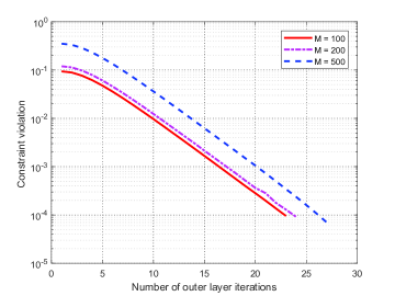
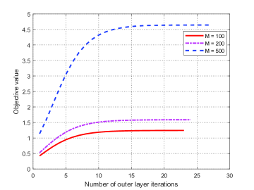
Before discussing the performance of the proposed schemes, we first verify the effectiveness of the proposed penalty-based Algorithm 2 for CSR. The constraint violation and convergence behaviour of Algorithm 2 are shown in Fig. 2 for one channel realization for different numbers of IRS reflecting elements $M$, namely, $M=100$, $M=200$, and $M=500$. From Fig. 2(a), it is observed that the constraint violation $\xi$ converges very fast to the predefined violation accuracy of $10^{-4}$ after about $23$ iterations for $M=100$, which indicates that equality constraints (29) and (30) in $\left({{\rm{\bar{P}}}1}\right)$ are eventually satisfied. Even for $M=500$, only $27$ iterations are required for reaching the predefined violation accuracy, which demonstrates the effectiveness of Algorithm 2. This can be observed more clearly in Fig. 2(b), where the penalized objective values of $\left({{\rm{\bar{P}}}1{\rm{-}}1}\right)$ obtained for different $M$ all increase quickly with the number of iterations and finally converge.

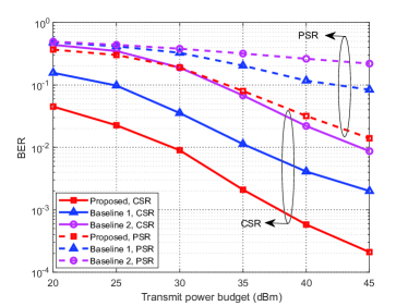
In order to evaluate the performance of the proposed IRS-based SR system, we compare the following schemes for CSR and PSR: 1) Proposed scheme: We jointly optimize the BS beamformer and phase shifts to minimize the BER of the IRS symbols. For CSR, Algorithm 2 is used, while for PSR, Algorithm 4 is applied; 2) Baseline Scheme $1$: we set ${\bf{w}}={{\sqrt{{P_{\max}}}{{\bf{h}}_{d}}}\mathord{\left/{\vphantom{{\sqrt{{P_{\max}}}{{\bf{h}}_{d}}}{\left\|{{{\bf{h}}_{d}}}\right\|}}}\right.\kern-1.2pt}{\left\|{{{\bf{h}}_{d}}}\right\|}}$ to achieve MRT for the BS-IR direct link, and the BER of the IRS symbols is minimized by optimizing the phase shifts; and 3) Baseline Scheme $2$: the IRS phase shifts are random and follow uniform distributions, and the BER of the IRS symbols is minimized by optimizing the BS beamformer. In Fig. 4, we compare the BER of the IRS symbols obtained for the above schemes versus $P_{\max}$ for $M=400$. Note that all results shown are obtained by simulation where we average $200$ channel realizations. As can be observed for all considered schemes, the BER of the IRS symbols decreases with $P_{\max}$. This is expected since from the objective functions of $(\rm P1)$ and $(\rm P2)$, it can be easily seen that as $P_{\max}$ grows, the SNR increases with the transmit power, thereby reducing the BER of the IRS symbols. In addition, for CSR, it is observed that the proposed scheme outperforms both Baseline Schemes $1$ and $2$, which demonstrates that the BER of the IRS symbols can indeed be reduced significantly with the joint BS beamformer and IRS phase shift optimization. A similar behavior is also observed for PSR. Furthermore, it is observed that the BER of the IRS symbols for CSR is significantly lower than that for PSR. This is because for CSR, one IRS symbols spans $L$ primary symbols. Thus, a diversity gain is obtained by exploiting MRT to coherently add up the multi-path signals to increase the SNR at the receiver. In contrast, for PSR, the period of the IRS symbol is equal to that of the primary symbol. Hence, the IRS reflected signals are treated as interference for the primary network, which thus degrades the system performance. In other words, the interference is harnessed in CSR, while it is harmful in PSR.

Figure 3: BER versus transmit power budget $P_{\max}$.

Figure 4: BER versus the number of IRS reflecting elements $M$.

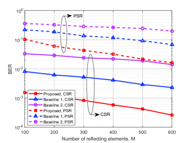
In Fig. 4, we show the BER of the IRS symbols versus the number of reflecting elements $M$. It is observed that the BER of the IRS symbols obtained by all considered schemes decreases with $M$. This is because more reflecting elements help achieve a higher passive beamforming gain, thereby improving the SNR. More importantly, since the IRS is passive with low power consumption and low hardware cost, it is promising to apply large IRSs with hundreds of reflecting elements. Moreover, for CSR, our proposed scheme outperforms Baseline Scheme $1$, which illustrates the benefits introduced by BS beamformer optimization. Furthermore, Baseline Scheme $2$ achieves some performance gains for CSR since the IRS is able to reflect some of the dissipated signals back to the receiver. A similar behavior is also observed for PSR. In addition, similar to Fig. 4, the BER of the IRS symbols obtained with CSR is lower than that obtained with PSR since the interference is harnessed in CSR.

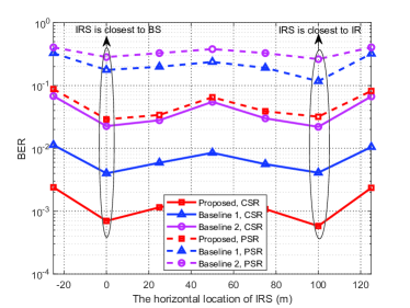
In Fig. 6, we study the impact of the IRS location on the BER of the IRS symbols for $M=400$. Specifically, we study the BERs obtained with the considered schemes versus the IRS’s horizontal location ($x$-coordinate), ranging from $-25~{}\rm m$ to $125~{}\rm m$. Note that for $x=0~{}\rm m$, the IRS is closest to the BS, while for $x=100~{}\rm m$, the IRS is closest to the IR. As can be observed, if the IRS is deployed close to the BS or IR, the BER decreases. This is because for a short distance between IRS and BS or IR, the signal attenuation in the BS-IRS-IR link is reduced due to the smaller double path loss [2]. Additionally, for CSR, the proposed scheme still outperforms Baseline Schemes $1$ and $2$. Similar results are also obtained for PSR. This further demonstrates the benefits of the proposed joint IRS phase shift and BS beamforming optimization.

Figure 5: The impact of IRS location on BER.

Figure 6: Outage probability versus $R_{\rm th}$.

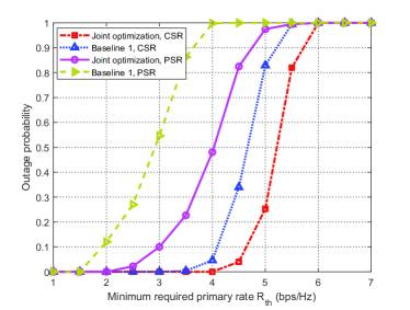
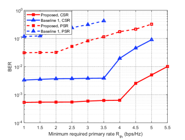
In Fig. 6, we plot the outage probability of the proposed schemes versus the required primary rate. For ease of exposition, we set $R_{csr,\rm th}=R_{psr,\rm th}=R_{\rm th}$. The outage probability is defined as the probability that the received primary rate at the IR is lower than a predefined minimum required primary rate $R_{\rm th}$. For the joint optimization scheme for CSR, we check the feasibility of $(\rm P1)$ by jointly optimizing the beamformer and the phase shifts, while for Baseline Scheme $1$, we optimize the phase shifts for the given MRT beamformer for the BS-IR link. For PSR, we make a similar comparisons for $(\rm P2)$. It is observed that the outage probability of all schemes increases with $R_{\rm th}$ and approaches $1$ for large $R_{\rm th}$. This is expected since the primary rate is upper bounded by a finite value due to the limited BS transmit power budget. For the CSR scenario, the joint optimization scheme has a lower outage probability than Baseline Scheme $1$, especially when $R_{\rm th}$ is larger than $4~{}{\rm bps/Hz}$. For example, the outage probability for the joint optimization scheme is about $0.042$ for $R_{\rm th}=4.5~{}{\rm bps/Hz}$, while that for Baseline Scheme $1$ is about $0.339$. This can also be deduced from $\left({{\rm{P}}1}\right)$. For any given phase shift $\bf v$, the left-hand-side of (23) obtained by optimizing the BS beamformer $\bf w$ is larger than that obtained by applying MRT, which indicates that the joint optimization scheme has a higher probability of satisfying constraint (23). For the PSR scenario, the joint optimization scheme has a lower outage probability than Baseline Scheme $1$. This can be deduced from $\left({{\rm{P}}2}\right)$. For any given phase shifts $\bf v$, the left-hand-side of (26) obtained by optimizing the BS beamformer $\bf w$ is larger than that obtained by applying MRT. In addition, the outage probability of the joint optimization scheme for CSR is lower than that for PSR. This can be readily derived from (23) and (26), where the left-hand-side of (23) is evidently larger than that of (26), which implies that a higher primary rate can be obtained with CSR. To see this more clearly, Fig. 7 studies the BER of the IRS symbols versus $R_{\rm th}$. It can be observed that for small $R_{\rm th}$, the BER remains nearly unchanged, while for large $R_{\rm th}$, the BER increases substantially. This is because as $R_{\rm th}$ becomes larger, the primary rate requirement constraint becomes stringent, so the optimization of the beamformer and phase shifts needs to fulfill the primary rate requirement at the cost of sacrificing the system performance.

Figure 7: BER versus $R_{\rm th}$.

VI Conclusion

In this paper, we have studied novel paradigms for IRS-based SR systems. Depending on the IRS’s symbol period, two scenarios, namely, CSR and PSR, have been considered with the objective of minimizing the BER of the IRS symbols by jointly optimizing the active beamformer at the base station and the phase shifts at the IRS while guaranteeing the minimum primary rate requirements. For the CSR scenario, we have decomposed the original problem into three subproblems, which allowed us to obtain semi-closed-form solutions for the BS beamformer and the IRS phase shifts. Then, a penalty-based algorithm with a two-stage iteration has been proposed to obtain a high-quality solution. For the PSR scenario, a bisection search based algorithm has been proposed. In particular, we have obtained a semi-closed-form solution for the BS beamformer, and leveraged the DC programming framework to obtain a rank-one solution. Our simulation results have shown that the proposed SR techniques achieve lower BERs as compared with two benchmark schemes and demonstrated that the BER can be significantly reduced by jointly optimizing the BS beamformer and IRS phase shifts for both scenarios. In addition, our results have also shown that the BER can be significantly reduced by proper positioning of the IRS, especially by placing the IRS close to the BS and/or IR. The results in this paper can be further extended by considering multiple IRSs, frequency-selective channel models, imperfect CSI, etc., which are interesting topics for future work in this area.

Appendix A Proof of Lemma 3

Define two dual variables $\tau_{1}$ and $\tau_{1}^{{}^{\prime}}$ corresponding to problem $\left({{\rm{\bar{P}}}2{\rm{-5}}}\right)$. Then, the corresponding beamforming vectors are denoted by ${{\bf{w}}\left({{\tau_{1}},\tau_{2}^{{\rm{opt}}}}\right)}$ and ${{\bf{w}}\left({\tau_{1}^{{}^{\prime}},\tau_{2}^{{\rm{{{}^{\prime}}opt}}}}\right)}$, respectively. In addition, we set $\tau_{1}>\tau_{1}^{{}^{\prime}}$. Since ${{\bf{w}}\left({{\tau_{1}},\tau_{2}^{{\rm{opt}}}}\right)}$ is the optimal beamformer with given ${{\tau_{1}}}$, we have

$${{\cal L}_{1}}\left({{\bf{w}}\left({{\tau_{1}},\tau_{2}^{{\rm{opt}}}}\right),{\tau_{1}}}\right)\geq{{\cal L}_{1}}\left({{\bf{w}}\left({\tau_{1}^{{}^{\prime}},\tau_{2}^{{\rm{{{}^{\prime}}opt}}}}\right),{\tau_{1}}}\right),$$ (79)

$${{\cal L}_{1}}\left({{\bf{w}}\left({\tau_{1}^{{}^{\prime}},\tau_{2}^{{\rm{{{}^{\prime}}opt}}}}\right),\tau_{1}^{{}^{\prime}}}\right)\geq{{\cal L}_{1}}\left({{\bf{w}}\left({\tau,\tau_{2}^{{\rm{opt}}}}\right),\tau_{1}^{{}^{\prime}}}\right).$$ (80)

Adding the above two inequalities, we have

$$\left({{\tau_{1}}-\tau_{1}^{{}^{\prime}}}\right)\left({{{\left\|{{\bf{w}}\left({\tau_{1}^{{}^{\prime}},\tau_{2}^{{\rm{{{}^{\prime}}opt}}}}\right)}\right\|}^{2}}-{{\left\|{{\bf{w}}\left({{\tau_{1}},\tau_{2}^{{\rm{opt}}}}\right)}\right\|}^{2}}}\right)\geq 0.$$ (81)

Since $\tau_{1}>\tau_{1}^{{}^{\prime}}$, we directly arrive at ${\left\|{{\bf{w}}\left({\tau_{1}^{{}^{\prime}},\tau_{2}^{{\rm{{{}^{\prime}}opt}}}}\right)}\right\|^{2}}\geq{\left\|{{\bf{w}}\left({{\tau_{1}},\tau_{2}^{{\rm{opt}}}}\right)}\right\|^{2}}$. This thus completes the proof.

References

• [1] M. Di Renzo, M. Debbah, D.-T. Phan-Huy, A. Zappone, M.-S. Alouini, C. Yuen, V. Sciancalepore, G. C. Alexandropoulos, J. Hoydis, H. Gacanin et al., “Smart radio environments empowered by reconfigurable AI meta-surfaces: An idea whose time has come,” EURASIP J. Wireless Commun. Netw., vol. 2019, no. 1, pp. 1–20, May 2019.
• [2] Q. Wu, S. Zhang, B. Zheng, C. You, and R. Zhang, “Intelligent reflecting surface aided wireless communications: A tutorial,” IEEE Trans. Commun., to appear, 2020.
• [3] C. Huang, S. Hu, G. C. Alexandropoulos, A. Zappone, C. Yuen, R. Zhang, M. Di Renzo, and M. Debbah, “Holographic MIMO surfaces for 6G wireless networks: Opportunities, challenges, and trends,” IEEE Wireless Commun., 2020, early access, doi: 10.1109/MWC.001.1900534.
• [4] Q. Wu and R. Zhang, “Towards smart and reconfigurable environment: Intelligent reflecting surface aided wireless network,” IEEE Commun. Mag., vol. 58, no. 1, pp. 106–112, Jan. 2020.
• [5] T. J. Cui, S. Liu, and L. Zhang, “Information metamaterials and metasurfaces,” J. Phys. Chem. C, vol. 5, no. 15, pp. 3644–3668, 2017.
• [6] B. O. Zhu, J. Zhao, and Y. Feng, “Active impedance metasurface with full 360 reflection phase tuning,” Scientific Reports, vol. 3, 2013.
• [7] Q. Wu and R. Zhang, “Intelligent reflecting surface enhanced wireless network via joint active and passive beamforming,” IEEE Trans. Wireless Commun., vol. 18, no. 11, pp. 5394–5409, Nov. 2019.
• [8] Q. Wu and R. Zhang, “Beamforming optimization for wireless network aided by intelligent reflecting surface with discrete phase shifts,” IEEE Trans. Commun., vol. 68, no. 3, pp. 1838–1851, Mar. 2020.
• [9] X. Guan, Q. Wu, and R. Zhang, “Intelligent reflecting surface assisted secrecy communication: Is artificial noise helpful or not?” IEEE Wireless Commun. Lett., vol. 9, no. 6, pp. 778–782, Jun. 2020.
• [10] Z. Zhang, L. Lv, Q. Wu, H. Deng, and J. Chen, “Robust and secure communications in intelligent reflecting surface assisted NOMA networks,” IEEE Commun. Lett., 2020, early access, doi: 10.1109/LCOMM.2020.3039811.
• [11] X. Yu, D. Xu, Y. Sun, D. W. K. Ng, and R. Schober, “Robust and secure wireless communications via intelligent reflecting surfaces,” IEEE J. Sel. Areas Commun., vol. 38, no. 11, pp. 2637–2652, Nov. 2020.
• [12] B. Feng, Y. Wu, M. Zheng, X.-G. Xia, Y. Wang, and C. Xiao, “Large intelligent surface aided physical layer security transmission,” IEEE Trans. Signal Process., vol. 68, pp. 5276–5291, 2020.
• [13] C. Pan, H. Ren, K. Wang, W. Xu, M. Elkashlan, A. Nallanathan, and L. Hanzo, “Multicell MIMO communications relying on intelligent reflecting surfaces,” IEEE Trans. Wireless Commun., vol. 19, no. 8, pp. 5218–5233, Aug. 2020.
• [14] M. Hua, Q. Wu, D. W. K. Ng, J. Zhao, and L. Yang, “Intelligent reflecting surface-aided joint processing coordinated multipoint transmission,” IEEE Trans. Commun., 2020, early access, doi: 10.1109/TCOMM.2020.3042275.
• [15] H. Xie, J. Xu, and Y. F. Liu, “Max-min fairness in IRS-aided multi-cell MISO systems with joint transmit and reflective beamforming,” IEEE Trans. Wireless Commun., 2020, early access, doi: 10.1109/TWC.2020.3033332.
• [16] Q. Wu and R. Zhang, “Weighted sum power maximization for intelligent reflecting surface aided SWIPT,” IEEE Wireless Commun. Lett., vol. 9, no. 5, pp. 586–590, May 2020.
• [17] C. Pan, H. Ren, K. Wang, M. Elkashlan, A. Nallanathan, J. Wang, and L. Hanzo, “Intelligent reflecting surface enhanced MIMO broadcasting for simultaneous wireless information and power transfer,” IEEE J. Sel. Areas Commun., vol. 38, no. 8, pp. 1719–1734, Aug. 2020.
• [18] Z. Li, W. Chen, and Q. Wu, “Joint beamforming design and power splitting optimization in IRS-assisted SWIPT NOMA networks,” 2020. [Online]. Available: https://arxiv.org/abs/2011.14778.
• [19] Y. Pan, K. Wang, C. Pan, H. Zhu, and J. Wang, “UAV-assisted and intelligent reflecting surfaces-supported terahertz communications,” 2020. [Online]. Available: https://arxiv.org/abs/2010.14223.
• [20] H. Long, M. Chen, Z. Yang, B. Wang, Z. Li, X. Yun, and M. Shikh-Bahaei, “Reflections in the sky: Joint trajectory and passive beamforming design for secure UAV networks with reconfigurable intelligent surface,” 2020. [Online]. Available: https://arxiv.org/abs/2005.10559.
• [21] S. Li, B. Duo, M. Di Renzo, M. Tao, and X. Yuan, “Robust secure UAV communications with the aid of reconfigurable intelligent surfaces,” 2020. [Online]. Available: https://arxiv.org/abs/2008.09404.
• [22] A. A. Boulogeorgos and A. Alexiou, “Performance analysis of reconfigurable intelligent surface-assisted wireless systems and comparison with relaying,” IEEE Access, vol. 8, pp. 94 463–94 483, 2020.
• [23] E. Björnson, Ö. Özdogan, and E. G. Larsson, “Intelligent reflecting surface versus decode-and-forward: How large surfaces are needed to beat relaying?” IEEE Wireless Commun. Lett., vol. 9, no. 2, pp. 244–248, Feb. 2019.
• [24] W. Yan, X. Yuan, Z. Q. He, and X. Kuai, “Passive beamforming and information transfer design for reconfigurable intelligent surfaces aided multiuser MIMO systems,” IEEE J. Sel. Areas Commun., vol. 38, no. 8, pp. 1793–1808, Aug. 2020.
• [25] W. Yan, X. Yuan, and X. Kuai, “Passive beamforming and information transfer via large intelligent surface,” IEEE Wireless Commun. Lett., vol. 9, no. 4, pp. 533–537, Apr. 2020.
• [26] J. Hu, Y.-C. Liang, and Y. Pei, “Reconfigurable intelligent surface enhanced multi-user MISO symbiotic radio system,” IEEE Trans. Commun., 2020, early access, doi: 10.1109/TCOMM.2020.3047444.
• [27] S. Lin, B. Zheng, G. C. Alexandropoulos, M. Wen, M. Di Renzo, and F. Chen, “Reconfigurable intelligent surfaces with reflection pattern modulation: Beamforming design and performance analysis,” IEEE Trans. Wireless Commun., 2020, early access, doi: 10.1109/TWC.2020.3028198.
• [28] Q. Zhang, Y. Liang, and H. V. Poor, “Large intelligent surface/antennas (LISA) assisted symbiotic radio for IoT communications,” 2020. [Online]. Available: https://arxiv.org/abs/2002.00340v1.
• [29] M. Hua, L. Yang, Q. Wu, C. Pan, C. Li, and A. L. Swindlehurst, “UAV-assisted intelligent reflecting surface symbiotic radio system,” 2020. [Online]. Available: https://arxiv.org/abs/2007.14029.
• [30] R. Y. Mesleh, H. Haas, S. Sinanovic, C. W. Ahn, and S. Yun, “Spatial modulation,” IEEE Trans. Veh. Technol., vol. 57, no. 4, pp. 2228–2241, Jul. 2008.
• [31] R. Long, Y.-C. Liang, H. Guo, G. Yang, and R. Zhang, “Symbiotic radio: A new communication paradigm for passive internet of things,” IEEE Internet of Things J., vol. 7, no. 2, pp. 1350–1363, Feb. 2019.
• [32] R. Long, H. Guo, L. Zhang, and Y.-C. Liang, “Full-duplex backscatter communications in symbiotic radio systems,” IEEE Access, vol. 7, pp. 21 597–21 608, 2019.
• [33] S. Zhang and R. Zhang, “Capacity characterization for intelligent reflecting surface aided MIMO communication,” IEEE J. Sel. Areas Commun., vol. 38, no. 8, pp. 1823–1838, Aug. 2020.
• [34] D. Tse and P. Viswanath, Fundamentals of Wireless Communication.   Cambridge university press, 2005.
• [35] S. M. Kay, Fundamentals of Statistical Signal Processing.   Prentice Hall PTR, 1993.
• [36] J. G. Proakis, Digital communication.   New York: McGraw-Hill, 1995.
• [37] S. Boyd and L. Vandenberghe, Convex Optimization.   Cambridge University Press, 2004.
• [38] J. Song, P. Babu, and D. P. Palomar, “Sequence design to minimize the weighted integrated and peak sidelobe levels,” IEEE Trans. Signal Process., vol. 64, no. 8, pp. 2051–2064, Apr. 2016.
• [39] Y. Sun, P. Babu, and D. P. Palomar, “Majorization-minimization algorithms in signal processing, communications, and machine learning,” IEEE Trans. Signal Process., vol. 65, no. 3, pp. 794–816, Feb. 2016.
• [40] Q. Shi, M. Hong, X. Gao, E. Song, Y. Cai, and W. Xu, “Joint source-relay design for full-duplex MIMO AF relay systems,” IEEE Trans. Signal Process., vol. 64, no. 23, pp. 6118–6131, Dec. 2016.
• [41] N. D. Sidiropoulos, T. N. Davidson, and Z.-Q. Luo, “Transmit beamforming for physical-layer multicasting,” IEEE Trans. Signal Process., vol. 54, no. 6, pp. 2239–2251, Jun. 2006.
• [42] P. D. Tao and L. T. H. An, “Convex analysis approach to DC programming: Theory, algorithms and applications,” Acta Math. Vietnamica, vol. 22, no. 1, pp. 289–355, 1997.
• [43] K. Yang, T. Jiang, Y. Shi, and Z. Ding, “Federated learning via over-the-air computation,” IEEE Trans. Wireless Commun., vol. 19, no. 3, pp. 2022–2035, Mar. 2020.
• [44] T. Jiang and Y. Shi, “Over-the-air computation via intelligent reflecting surfaces,” in Proc. 2019 IEEE Global Communications Conference (GLOBECOM), pp. 1–6.
• [45] X. Yu, D. Xu, D. W. K. Ng, and R. Schober, “IRS-assisted green communication systems: Provable convergence and robust optimization,” 2020. [Online]. Available: https://arxiv.org/abs/2011.06484.