Multifractality and Fock-space localization in many-body localized states:
one-particle density matrix perspective

Abstract

Many-body localization (MBL) is well characterized in Fock space. To quantify the degree of this Fock space localization, the multifractal dimension $D_{q}$ is employed; it has been claimed that $D_{q}$ shows a jump from the delocalized value $D_{q}=1$ in the ETH phase (ETH: eigenstate thermalization hypothesis) to a smaller value $0<D_{q}<1$ at the ETH-MBL transition, yet exhibiting a conspicuous discrepancy from the fully localized value $D_{q}=0$, which indicate that multifractality remains inside the MBL phase. Here, to better quantify the situation we employ, instead of the commonly used computational basis, the one-particle density matrix (OPDM) and use its eigenstates (natural orbitals) as a Fock state basis for representing many-body eigenstates $|\psi\rangle$ of the system. Using this basis, we compute $D_{q}$ and other indices quantifying the Fock space localization, such as the local purity $S$, which is derived from the occupation spectrum $\{n_{\alpha}\}$ (eigenvalues of the OPDM). We highlight the statistical distribution of Hamming distance $x_{\mu\nu}$ occurring in the pair-wise coefficients $|a_{\mu}|^{2}|a_{\nu}|^{2}$ in $S$, and compare this with a related quantity considered in the literature.

I Introduction

A many-body, i.e., interacting system tends to thermalize under its own dynamics, Deutsch (1991); Srednicki (1994); Rigol et al. (2008); D’Alessio et al. (2016) and at weak disorder realizes delocalized eigenstates. However, in the regime of strong disorder, the so-called local integrals of motion (LIOMs) Serbyn et al. (2013a); Huse et al. (2014); Ros et al. (2015) are emergent and hinder thermalization and transport in the system, leading the system to a many-body localization (MBL) phase. The existence of such an intriguing phase was first suggested theoretically,Basko et al. (2006) then supported by experiments mainly in cold-atom systems. Schreiber et al. (2015); Choi et al. (2016); Smith et al. (2016); Roushan et al. (2017); Xu et al. (2018) Emergence of the LIOMs in the MBL phase leads to various unusual properties of the MBL phase, Imbrie et al. (2017) such as Poisson level statistics,Oganesyan and Huse (2007) area-law behavior of the entanglement entropy,Bauer and Nayak (2013); Khemani et al. (2017) and its very slow (logarithmic) spreading in time,Žnidarič et al. (2008); Bardarson et al. (2012); Serbyn et al. (2013b) etc. While the Anderson localization Anderson (1958) for a non-interacting system occurs in the real space, MBL can be regarded as localization in the Fock space. Altshuler et al. (1997); Roy et al. (2019); Roy and Logan (2020) After intensive study in the last decade both from theoretical and experimental sides, the basic understanding on the physics of MBL has now been established. Nandkishore and Huse (2015); Altman and Vosk (2015); Alet and Laflorencie (2018); Abanin et al. (2019)

In the regime of weak disorder delocalized eigenstates follow the eigenstate thermalization hypothesis (ETH) Deutsch (1991); Srednicki (1994); Rigol et al. (2008); D’Alessio et al. (2016); i.e., the eigenstates are also delocalized in the Fock space, realizing effectively a micro-canonical ensemble; under such a circumstance the expectation value of a local observable, e.g., the local magnetization,Luitz (2016) takes a well-defined thermodynamic value in a given energy window between $E$ and $E+\Delta E$. In the MBL phase, on the other hand, realized eigenstates involve only a fraction of the available Fock space, and in the extremely localized limit, the eigenstates become a simple product of LIOM orbitals, i.e., the Anderson localization orbitals dressed by the interaction. In such a MBL phase, the system is no longer in equilibrium, and the expectation value of local observables fluctuate.Luitz (2016) To quantify such different situations in the ETH and MBL phases, one considers the inverse participation ratio (IPR) in the Fock space [defined in Eq. (38)], or a related quantity, the multifractal dimension $D_{q}$ [defined in Eq. (39)]. Note that $D_{q}=1$ for a fully delocalized state, while $D_{q}=0$ for a fully localized state, and the intermediate situation: $0<D_{q}<1$ is called multifractal. In non-interacting higher dimensional systems delocalization-localization occurs at a single point, and only at this point the system becomes multifractal ($0<D_{q}<1$). Here, in 1D interacting systems the situation is rather different; preceding works Tikhonov and Mirlin (2018); Tarzia (2020); Luitz et al. (2020); Macé et al. (2019); Tomasi et al. (2020) have suggested that $D_{q}=1$ in the ETH phase, while after the ETH-MBL transition $D_{q}$ remains multifractal ($0<D_{q}<1$), reflecting the many-body nature of the system; i.e., at the ETH-MBL transition $D_{q}$ does not show a complete transition to the ideal value $D_{q}=0$ corresponding to true localization as far as the disorder strength is finite. Still, $D_{q}$ shows a partial discontinuity at the ETH-MBL transition, and a similar discontinuity is also expected in the entanglement entropy. De Tomasi and Khaymovich (2020); Tomasi et al. (2020) In Refs. Laflorencie et al., 2020; Tomasi et al., 2020 the meaning of the finiteness of $D_{q}$ in the MBL phase has been analyzed, and its relation to the nature of ETH-MBL phase transition is discussed; the latter is claimed to be KT-like.Dumitrescu et al. (2019) In the MBL phase $D_{q}$ also strongly fluctuates, and said to be non self-averaging.Solórzano et al. (2021) In the avalanche scenario, proposed in Refs. Thiery et al., 2018; Luitz et al., 2017; De Roeck and Huveneers, 2017 the multifractalty in the MBL phase may be given the following natural interpretation: in a generic situation in the MBL phase LIOMs are formed, but some “spins” are still active in the pseudospin picture; i.e., LIOMs are not precisely good quantum numbers. It is natural to presume that under such circumstances a many-body eigenstate is only partially localized in the Fock space (IPR$\neq 1$, $D_{q}\neq 0$). When disorder is no longer strong enough, the density of active spins reaches a certain threshold value, at which an avalanche of active spins occurs, destroying (melting) completely the frozen LIOMs, resulting in the ETH situation: IPR$\simeq 0$, $D_{q}\simeq 1$.

Here, in the remainder of the paper we focus on this intriguing partial localization in the Fock space in the generic MBL phase. To what extent a many-body eigenstate $|\psi\rangle$ in Eq. (2) is localized in the Fock space depends on the basis one employs for representing $|\psi\rangle$. In numerics, one a priori employs the computational basis (4), in which the coefficients $a_{\{n_{j}\}}$ in Eq. (2) show a rather broad distribution; i.e., $|\psi\rangle$ is not much localized in the corresponding Fock space even in the MBL phase and even in the theoretical LIOM limit. To quantify the degree of Fock-space localization in the MBL phase more properly, it is ideal to employ the basis of LIOM orbitals, but this is not straightforward, since in a generic MBL situation LIOMs are coupled to a thermal bath; not commuting with the total Hamiltonian, they are no longer in the strict sense integrals of the motion.Luitz et al. (2017) Under such circumstances, instead of seeking for constructing LIOMs, it may be more realistic to employ the eigenstates of the one-particle density matrix (OPDM).Bera et al. (2015, 2017) Under an assumption in the deep MBL phase (see Sec. II-B) the eigenvectors of OPDM, called natural orbitals, are shown to coincide with the LIOMs. In a more generic situation in the MBL phase they are assumed to be still good approximations of the LIOMs. The OPDM approach has been employed in the study of MBL in various models Villalonga et al. (2018); Lin et al. (2018); Macé et al. (2019); Chen et al. (2020); Orito et al. (2020); Hopjan and Heidrich-Meisner (2020) and in the study of out-of-equilibrium phenomena. Lezama et al. (2017); Hopjan et al. (2020)

In this work, we have computed $D_{q}$ and other indices quantifying the Fock space localization in the OPDM and other bases, and have compared the results. With the use of OPDM basis, mimicking the LIOM basis, one can remove, or at least minimize effects of the finiteness of Fock-space localization length, which manifests, e.g., in the finiteness of $D_{q}$ in the MBL phase. We expect that this will result in a better description of the ETH-MBL transition/crossover regime. Our analyses in the OPDM basis show that the finiteness of $D_{q}$ in the computational basis reported in the literature is indeed due to the finiteness of the Fock-space localization length. The eigenenergies $\rho_{\alpha}$ of the OPDM (occupation spectrum) shows a characteristic gapped distribution in the MBL phase, reminiscent of a renormalized Fermi distribution in Fermi liquids. Bera et al. (2015) In the idealized LIOM case, this becomes a simple step function as in Fermi gas, indicating that the corresponding many-body state $|\psi\rangle$ can be expressed by a single Slater determinant. Thus, the degree of Fock-space localization is encoded in how close the occupation spectrum is to a simple step function. Or, one can numerate this resemblance to a step function by a single index, called the local purity.Viola and Brown (2007)

The remainder of the paper is organized as follows. In Sec. II we highlight various aspects of the OPDM approach to many-body localization with a particular emphasis on the behavior of occupation spectrum and Fock-space IPR. and, in Sec. III we introduce the quantity called local purity, an index quantifying the nature of occupation spectrum. We compare the behavior of the local purity with that of the Fock-space IPR from the viewpoint of the distribution of Hamming distance $x_{\mu\nu}$ in the pairwise coefficients $|a_{\mu}|^{2}|a_{\nu}|^{2}$. Sec. IV is devoted to Concluding Remarks. Some details are postponed to three sections in the Appendices.

II The OPDM approach to MBL

To fix the notation let us first introduce our model:

$$H=\sum_{j=1}^{L}\Big{[}-t(c_{j+1}^{\dagger}c_{j}+c_{j}^{\dagger}c_{j+1})+W_{j}\left(\hat{n}_{j}-\frac{1}{2}\right)$$

$$+V\left(\hat{n}_{j}-\frac{1}{2}\right)\left(\hat{n}_{j+1}-\frac{1}{2}\right)\Big{]},$$ (1)

where $j$ represents a site in real space, and $L$ is the size of the system. $c_{j}^{\dagger}$ ($c_{j}$) creates (annihirates) an electron at site $j$, and $\hat{n}_{j}=c_{j}^{\dagger}c_{j}$ counts the local electron density at site $j$. In the first two terms of Eq. (1), $t$ represents the strength of hopping between the nearest-neighbor sites, and in the third term the strength $W_{j}$ of the on-site impurity potential is a random variable at each site $j$ and each obeys the uniform distribution of magnitude $W$; $W_{j}\in[-W,W]$. In the second line $V$ represents the strength of nearest-neighbor interaction. The system prescribed by Eq. (1) represents one of the paradigmatic models for describing the many-body localization phenomenon. Abanin et al. (2019) The on-site potential term of strength $W$ tends to localize the electronic wave functions, while the hopping and the interaction terms, each parametrized, respectively, by $t$ and $V$, tend to delocalize them. The competition of these three different types of contributions, each represented by the parameters, $t$, $W$ and $V$, determine the localization/delocalization feature of the system (cf. e.g., the phase diagram of Ref. Luitz et al., 2015. Note that in Eq. (1) we presume a periodic boundary condition so that $c_{j+L}\equiv c_{j}$.

Figure 1: The occupation spectrum $\{\overline{\rho_{\alpha}}\}$ [panels (a)-(c)] and the corresponding probability distribution $P(\rho_{\alpha})$ [panels (d)-(f)] in different many-body bases [(a), (d): the computational, (b), (e): the AL orbital, and (c), (f): the OPDM bases].

A generic many-body eigenstate $|\psi\rangle$ of the Hamiltonian such as Eq. (1), satisfying $H|\psi\rangle=E|\psi\rangle$, takes the following form:

$$|\psi\rangle = \sum_{\{n_{j}\}}a_{\{n_{j}\}}|\{n_{j}\}\rangle,$$ (2)

i.e., a superposition of

$$N=\frac{L!}{N_{e}!(L-N_{e})!}$$ (3)

different electron configurations:

$$|\{n_{j}\}\rangle \equiv |n_{1}n_{2}\cdots n_{L}\rangle$$ (4)

$$= (c_{L}^{\dagger})^{n_{L}}\cdots(c_{2}^{\dagger})^{n_{2}}(c_{1}^{\dagger})^{n_{1}}|0\rangle,$$

with a suitable weight $a_{\{n_{j}\}}$. The notation $\{n_{j}\}$ specifies a Fock representation:

$$\{n_{j}\}=(n_{1},n_{2},\cdots,n_{L}),$$ (5)

where $n_{j}=0,1$ (fermionic statistics), and $c_{j}^{\dagger}$ creates an electron on a site $j$. $\sum_{j=1}^{L}n_{j}=N_{e}$ represents the number of electrons. In numerics, the many-body basis (4) is usually employed; therefore dubbed as computational basis. In the following we focus on the typical case of half-filling: $N_{e}=L/2$. In numerical simulations we also set the parameters at the following typical values: $t=1/2$ and $V=1$.

II.1 The OPDM and its eigenvalues (the occupation spectrum)

For a given many-body eigenstate $|\psi\rangle$ we introduce a one-particle density matrix (OPDM) $\rho$ whose $(i,j)$-element $\rho_{ij}$ is defined as

$$\rho_{ij}=\langle\psi|c_{i}^{\dagger}c_{j}|\psi\rangle,$$ (6)

where $i,j=1,2,\cdots,L$ represent a site in real space. We then diagonalize the $L\times L$ matrix $\rho$ (i.e., the OPDM) so that

$$\rho u^{(\alpha)}=\rho_{\alpha}u^{(\alpha)}.$$ (7)

The set of eigenvalues $\rho_{\alpha}$ is called the occupation spectrum, while the corresponding eigenstates are called natural orbitals $u^{(\alpha)}$ (for reasons that will become clear below). Bera et al. (2015, 2017)

Creating an electron in the $\alpha$th natural orbital,

$$u^{(\alpha)}=(u^{(\alpha)}_{1},u^{(\alpha)}_{2},\cdots,u^{(\alpha)}_{L})^{t}$$ (8)

can be represented by a creation operator,

$$c_{\alpha}^{\dagger}=\sum_{j=1}^{L}u^{(\alpha)*}_{j}c_{j}^{\dagger}.$$ (9)

The occupation of the $\alpha$th natural orbital in the many-body eigenstate $|\psi\rangle$ is specified by the quantity:

$$\langle\psi|c_{\alpha}^{\dagger}c_{\alpha}|\psi\rangle=\sum_{ij}u^{(\alpha)*}_{i}u^{(\alpha)}_{j}\langle\psi|c_{i}^{\dagger}c_{j}|\psi\rangle,$$ (10)

but recalling the definitions of the OPDM $\rho$ and of the natural orbitals $u_{\alpha}$ [Eq. (6) and Eq. (7)], one immediately finds that this is identical to $\rho_{\alpha}$ given in Eq. (7). Thus, the set of eigenvalues,

$$\{\rho_{\alpha}\}=(\rho_{\alpha_{1}},n_{\alpha_{2}},\cdots,\rho_{\alpha_{L}})$$ (11)

of the OPDM $\rho$ specifies how $L$ natural orbitals $u^{(\alpha)}$ are occupied in the state $|\psi\rangle$.

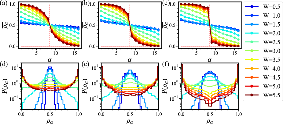
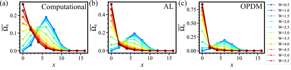
The occupation spectrum $\{\rho_{\alpha}\}$ computed in the OPDM (natural orbital) basis is shown in Fig. 1 (c). The set of OPDM eigenvalues $\{\rho_{\alpha}\}$ is obtained by numerically diagonalizing the matrix $\rho$ for a state $|\psi\rangle$, then we have labelled them in the descending order of $\rho_{\alpha}$ such that

$$\rho_{\alpha_{1}}>\rho_{\alpha_{2}}>\cdots>\rho_{\alpha_{L}}.$$ (12)

We repeat this procedure for different eigenstates $|\psi\rangle$ in the middle of the spectrum, then for different disorder configurations. Each component $\rho_{\alpha}$ in the set $\{\rho_{\alpha}\}$ is then averaged over different samples: $\rho_{\alpha}\rightarrow\overline{\rho_{\alpha}}$, and the sample-averaged occupation spectrum:

$$[\overline{\rho_{\alpha}}]=\left(\overline{\rho_{\alpha_{1}}},\overline{\rho_{\alpha_{2}}},\cdots,\overline{\rho_{\alpha_{L}}}\right)$$ (13)

is found, where $\overline{\cdots}$ represents sample averaging. In Fig. 1 (c) we have repeated this calculation for different disorder strength $W$, and at each value of $W$ we have plotted the sample-averaged occupation spectrum $[\overline{\rho_{\alpha}}]$ as a function of $\alpha$. At each value of $W\geq 2.5$, we have averaged in total over $5\times 10^{3}$ samples.

In the deep MBL regime: $W\gg 3.5$, $\rho_{\alpha}$ shows a sharp jump $\Delta\rho_{\alpha}$ from $\alpha=L/2$ to $\alpha=L/2+1$; the entire shape of the spectrum is close to the form of a step function; i.e.,

$$\rho_{\alpha} = \theta(\alpha-L/2)$$ (16)

$$= \left\{\begin{array}[]{ll}1&({\rm for}\ \alpha>L/2)\\ 0&({\rm for}\ \alpha\leq L/2)\end{array}\right..$$

As $W$ decreases, the magnitude of the jump $\Delta\rho_{\alpha}$ diminishes, and the spectrum $\rho_{\alpha}$ tends to become a smooth function that varies only in a small range of values around $\rho_{\alpha}=0.5$ in the ETH regime: $W\ll 3.5$.

How close the shape of the occupation spectrum is to a step function (16) is a measure of how close the given many-body eigenstate $|\psi\rangle$ is to a simple product state; i.e., to what extent the state is Fock-space localized in the basis chosen. If the state $|\psi\rangle$ is expressed in some basis as a simple product state:

$$|\psi\rangle=\gamma_{\beta_{L/2}}^{\dagger}\cdots\gamma_{\beta_{2}}^{\dagger}\gamma_{\beta_{1}}^{\dagger}|0\rangle\equiv|[\beta_{0}]\rangle_{\rm LIOM},$$ (17)

where $\gamma_{\beta}^{\dagger}$ creates an electron in the $\beta$th orbital in this basis, and if one measures the occupation spectrum $\rho_{\beta}$ in the same basis, then the occupation

$$\rho_{\beta}=\langle\psi|\gamma_{\beta}^{\dagger}\gamma_{\beta}|\psi\rangle$$ (18)

becomes a simple step function as Eq. (16), since in this case $\{\rho_{\beta}\}$ reduces to the simple Fock representation:

$$\{n_{\beta}\} = (n_{\beta_{1}},\cdots,n_{\beta_{L/2}},n_{\beta_{L/2+1}},\cdots,n_{\beta_{L}})$$ (19)

$$= (1,\cdots,1,0,\cdots,0)$$

of the state $|[\beta_{0}]\rangle_{\rm LIOM}$; i.e., $n_{\beta}=1$ if $\beta$ is occupied, while $n_{\beta}=0$ othehrwise. The last line holds if the orbitals $\beta$ are arranged in the descending order of $n_{\beta}$.

II.2 Relation to LIOM, comparison with other bases

In the deep MBL regime in which the local integrals of motion (LIOMs) become good quantum numbers, the many-body eigenstate $|\psi\rangle$ can be expressed as a single Slater determinant as in Eq. (17) in terms of the LIOM creation operators:Bera et al. (2017)

$$\gamma_{\alpha}^{\dagger}=\sum_{i}A^{(\alpha)*}_{i}c_{i}^{\dagger}+\sum_{ijk}B^{(\alpha)*}_{ijk}c_{i}^{\dagger}c_{j}^{\dagger}c_{k}+\cdots,$$ (20)

where $A^{(\alpha)}_{j}$ represents the principal part of the LIOM wave function, while $B^{(\alpha)*}_{ijk}$ represents a correction associate with a particle-hole excitation. $\cdots$ represents higher-order corrections that stem from higher-order terms in the perturbative expansion of LIOM. Here, we consider the extremely localized limit, and hypothesize that only the first term of Eq. (20) is relevant, and neglect the terms of order higher than two.Tomasi et al. (2020) Then, it is natural to assume that the amplitudes $A^{(\alpha)}_{j}$ are orthonormal:

$$\sum_{i}A^{(\alpha)*}_{i}A^{(\beta)}_{i}=\delta_{\alpha\beta},\ \ \sum_{\alpha}A^{(\alpha)}_{i}A^{(\alpha)*}_{j}=\delta_{ij},$$ (21)

since they are simply LIOM wave functions. Using Eq. (21), one can invert Eq. (20) as

$$c_{i}^{\dagger}\simeq\sum_{\alpha}A^{(\alpha)}_{i}\gamma_{\alpha}^{\dagger}.$$ (22)

Then, the OPDM matrix $\rho$ [Eq. (6)] becomes

$$\rho_{ij} = \langle\psi|c_{i}^{\dagger}c_{j}|\psi\rangle$$ (23)

$$\simeq \sum_{\alpha\beta}A^{(\alpha)}_{i}A^{(\beta)*}_{j}\langle\psi|\gamma_{\alpha}^{\dagger}\gamma_{\beta}|\psi\rangle$$

$$= \sum_{\alpha}n_{\alpha}A^{(\alpha)}_{i}A^{(\alpha)*}_{j}=\sum_{\alpha:{\rm occupied}}A^{(\alpha)}_{i}A^{(\alpha)*}_{j}.$$

In the intermediate step, we have used

$$\langle\psi|\gamma_{\alpha}^{\dagger}\gamma_{\beta}|\psi\rangle=n_{\alpha}\delta_{\alpha\beta},$$ (24)

where $n_{\alpha}$’s are as given in Eq. (19). Note that Eq. (23) is nothing but the spectral decomposition of the OPDM matrix $\rho$ such that

$$\rho_{ij}=\sum_{\alpha}\rho_{\alpha}u^{(\alpha)}_{i}u^{(\alpha)*}_{j},$$ (25)

in the case of $\rho_{\alpha}=n_{\alpha}$. This signifies that the LIOM orbitals $A^{(\alpha)}_{j}$ are identical to natural orbitals $u^{(\alpha)}_{j}$ in this limit, and the corresponding occupation spectrum $\{\rho_{\alpha}\}$ reduces to a simple occupation $\{n_{\alpha}\}$ [i.e., the Fock representation as given in Eq. (19)] of LIOM orbitals; the latter becomes a simple step function as given in Eq. (16).

In a generic situation in the MBL phase, the LIOM creation operator (20) will be still valid, but higher order terms therein may play some role. In this case the natural orbitals are no longer identical to LIOM orbitals but still close to them, and the occupation spectrum $\{\rho_{\alpha}\}$ is no longer an ideal step function but still shows a jump $\Delta\rho_{\alpha}<1$ from $\alpha=L/2$ to $\alpha=L/2+1$. Such features can indeed be seen in Fig. 1 (c) in the deep MBL regime: $W\gg 3.5$.

Panels (a) and (b) of Fig. 1 show the occupation spectrum $\{\rho_{\alpha}\}$ calculated (a) in the computational, and (b) in the AL orbital bases, for comparison. In cases (a) and (b),

$$\rho_{j} = \langle\psi|c_{j}^{\dagger}c_{j}|\psi\rangle=\rho_{jj},$$

$$\rho_{\alpha}^{(AL)} = \langle\psi|c_{AL}^{(\alpha)\dagger}c_{AL}^{(\alpha)}|\psi\rangle$$ (26)

$$= \sum_{ij}\psi_{AL}^{(\alpha)*}(i)\psi_{AL}^{(\alpha)}(j)\rho_{ij}$$

have been calculated, respectively, and then sample-averaged, where $\rho_{ij}$ is the OPDM matrix, and

$$c_{AL}^{(\alpha)\dagger}=\sum_{j=1}^{L}\psi_{AL}^{(\alpha)*}(j)c_{j}^{\dagger},$$ (27)

creates an electron in the $\alpha$th AL orbital $\psi_{AL}^{(\alpha)}$.

In the ETH regime ($W$: small $\ll 3.5$) the occupation spectrum $\rho_{\alpha}$ becomes a smooth function that varies only in a small range of values around $\rho_{\alpha}=0.5$ in all the three bases; i.e., the local observable $\overline{\rho_{\alpha}}$ exhibits a well-defined thermodynamical value at a given energy (for a given $|\psi\rangle$), realizing a situation consistent with the hypothesis of ETH. In the MBL regime ($W$: large $\gg 3.5$), on the other hand, the values of $\overline{\rho_{\alpha}}$ differ on the two sides of the jump at $\alpha=L/2$, breaking the hypothesis of ETH. This also implies localization in the Fock space.

In the deep MBL regime: $W\gg 3.5$, the occupation spectrum $\rho_{\alpha}$ is closest to a step function in (c) the OPDM (natural orbital) basis, indicating that in this basis the many-body eigenstate is predominantly described by a single Slater determinant. This also implies that the corresponding natural orbitals are close to those of LIOMs. In cases of (a) and (b), the occupation spectrum $\rho_{\alpha}$ deviates significantly from a simple step function; the AL orbitals [case of panel (b)] and those of the computational basis; i.e., $\psi_{j}(x)=\delta(x-j)$, are not particularly close to LIOM orbitals.

II.3 Probability distribution of $\rho_{\alpha}$

To see why the occupation spectrum $\rho_{\alpha}$ deviates significantly, especially, in cases of (a) and (b), from a simple step function, even in the MBL phase, we then consider the (statistical) distribution of $\rho_{\alpha}$ in each and different realizations; here we cease to order $\rho_{\alpha}$’s in each realization [as in Eq. (12)] and focus on the occurrence of the quantal expectation value (26) in cases (a) and (b) and the eigenvalue $\rho_{\alpha}$ of the OPDM [Eq. (7)] for $\alpha=1,2,\cdots,L$ and in different realizations and its distribution in the range $[0,1]$. We have counted the number of occurrences $\rho_{\alpha}$ in the bins $[\rho_{\alpha},\rho_{\alpha}+\Delta\rho_{\alpha}]$, and establish a histogram of $\rho_{\alpha}$; then after normalization one finds the distribution $P(\rho_{\alpha})$.

In the ETH limit the distribution $P(\rho_{\alpha})$ is expected to be a narrow gaussian function centered at $\rho_{\alpha}=1/2$, while in the deep MBL phase $\rho_{\alpha}$ takes either 0 or 1; as a result $P(\rho_{\alpha})$ is expected to become a bimodal function sharply peaked at 0 and 1. In Fig. 1 we show such distribution $P(\rho_{\alpha})$, (d) in the computational, (e) in the Anderson localization orbital, and (f) in the OPDM (natural orbital) bases. The width of the bins is chosen as $\Delta\rho_{\alpha}=1/40$. At weak $W$, in the ETH regime: $W\ll 3.5$, the distribution $P(\rho_{\alpha})$ shows a peak centered at $\rho_{\alpha}=1/2$ in all three different bases, while the peak broadens as $W$ increases. In the MBL regime: $W\gg 3.5$, $P(\rho_{\alpha})$ becomes a bimodal function peaked at 0 and 1, but with a relatively long tail, in cases of (d) and (e), extended toward the center of the distribution $\rho_{\alpha}=1/2$.

The reason why $\rho_{\alpha}$ takes such values away from the extreme values 0 and 1 is that the LIOM wave function has a finite localization length even in the deep MBL phase. In the LIOM limit the many-body eigenstate $|\psi\rangle$ is expressed by a simple product state as in Eq. (17), in which $\gamma_{\alpha}^{\dagger}$ represents a LIOM creation operator as in Eq. (20). Then, the occupation $\langle n_{j}\rangle$ in the computational basis can be expressed as a superposition of LIOM orbitals as

$$\rho_{j}=\langle\psi|c_{j}^{\dagger}c_{j}|\psi\rangle\simeq\sum_{\alpha:{\rm occupied}}|A^{(\alpha)}_{j}|^{2},$$ (28)

where, for simplicity, we have kept only the first term of Eq. (20), and have neglected the higher order terms. In this case the creation operator $c_{j}^{\dagger}$ in the computational basis can be written as in Eq. (22). The LIOM orbital $A^{(\alpha)}_{j}$ has a finite spread in real space; i.e., a finite localization length $\xi_{\alpha}$ such that Laflorencie et al. (2020)

$$A^{(\alpha)}_{j}\simeq\sqrt{\tanh\frac{1}{2\xi_{\alpha}}}\exp\left(-\frac{|j-j_{\alpha}|}{2\xi_{\alpha}}\right),$$ (29)

which indicates that Eq. (28) represents a superposition of exponentially decaying amplitudes centered at localization centers $j_{\alpha}$. At a generic site $j$, contributions of the tails from different localization centers $j_{\alpha}$ superpose and give a finite amplitude, where $\alpha\in$ occupied states. The distribution $P(\langle n_{j}\rangle)$ in this case is expected to have a relatively long tail away from the extreme values $\langle n_{j}\rangle=0,1$.

In the AL orbital basis, one measures, instead of $c_{j}^{\dagger}$, $c_{AL}^{(\alpha)\dagger}$ given in Eq. (27). Here, in the LIOM limit, using Eq. (22), one rewrites Eq. (27) as

$$c_{AL}^{(\alpha)\dagger} = \sum_{j=1}^{L}\psi_{AL}^{(\alpha)*}(j)c_{j}^{\dagger}$$ (30)

$$= \sum_{j,\beta}\psi_{AL}^{(\alpha)*}(j)A^{(\beta)}_{j}\gamma_{\beta}^{\dagger}=\sum_{\beta}\tilde{A}^{(\beta)}_{\alpha}\gamma_{\beta}^{\dagger},$$

where we have introduced the amplitude

$$\tilde{A}^{(\beta)}_{\alpha}=\sum_{j}\psi_{AL}^{(\alpha)*}(j)A^{(\beta)}_{j}.$$ (31)

Clearly, $\tilde{A}^{(\beta)}_{\alpha}$ represents the overlap of the $\alpha$th AL orbital and $\beta$th LIOM orbital. In the non-interacting limit, the orbitals coincide so that Eq. (31) reduces to an orthogonality relation: $\tilde{A}^{(\beta)}_{\alpha}=\delta_{\alpha\beta}$. In case of $V\neq 0$, $\tilde{A}^{(\beta)}_{\alpha}$ is no longer $\delta_{\alpha\beta}$, but is still close. In the reversed relation:

$$\gamma_{\beta}^{\dagger}=\sum_{\alpha}\tilde{A}^{(\beta)*}_{\alpha}c_{AL}^{(\alpha)\dagger},$$ (32)

$\tilde{A}^{(\beta)}_{\alpha}$ can be also regarded as the amplitude of $\beta$th LIOM wave function in the AL orbital basis $\alpha$. The LIOM wave function $A^{(\alpha)}_{j}$ has a finite spread in the real space basis $j$ as in Eq. (29), while in the AL orbital basis $\tilde{A}^{(\beta)}_{\alpha}$ is closer to a $\delta$-function $\delta_{\alpha\beta}$; at least it will be more localized than in the real space basis. Using Eq. (30), one can express the occupation $\rho_{\alpha}^{(AL)}$ of the $\alpha$th AL orbital as

$$\rho_{\alpha}^{(AL)}=\langle\psi|c_{AL}^{(\alpha)\dagger}c_{AL}^{(\alpha)}|\psi\rangle\simeq\sum_{\beta:{\rm occupied}}|\tilde{A}^{(\beta)}_{\alpha}|^{2},$$ (33)

i.e., in the form of a superposition of localized orbitals as in Eq. (28). The difference is that here each contribution is more localized in the space of AL orbitals; therefore, the distribution $P(\rho_{\alpha}^{(AL)})$ is expected to have a larger weight in the vicinity of two extreme values $\rho_{\alpha}^{(AL)}=0,1$.

In the case of OPDM basis, if one considers the same LIOM limit under the hypothesis of neglecting the higher order terms of Eq. (20), then the natural orbitals $u^{(\alpha)}_{j}$ are shown to be identical to LIOM wave functions $A^{(\alpha)}_{j}$. As compared to the case of AL orbital basis, $\psi_{AL}^{(\alpha)*}(j)$ should be replaced with $u^{(\alpha)*}_{j}$ in the expression for $\tilde{A}^{(\beta)}_{\alpha}$ in Eq. (31). Then, $u^{(\alpha)}_{j}=A^{(\alpha)}_{j}$ signifies

$$\tilde{A}^{(\beta)}_{\alpha}=\sum_{j}u^{(\alpha)*}_{j}A^{(\beta)}_{j}=\delta_{\alpha\beta},$$ (34)

i.e., the LIOM wave function $\tilde{A}^{(\beta)}_{\alpha}$ is ultimately localized in the OPDM basis. Conferring to Eq. (33), this implies that the distribution $P(\rho_{\alpha})$ in the OPDM basis becomes a ultimately sharp bimodal function peaked at $\rho_{\alpha}=0,1$. Of course, in reality the higher order terms of Eq. (20) play some role, so that Eq. (34) does not literally hold. As a result, $P(\rho_{\alpha})$ still has some weights (though much suppressed) away from the extreme values $\rho_{\alpha}=0,1$.

In the MBL phase, $P(\rho_{\alpha})$ is a U-shaped function in cases of (a) and (b), showing a broad minimum around $\rho_{\alpha}=1/2$, while in case (c), as $W$ increases, a dip evolves at $\rho_{\alpha}=1/2$, deforming the global shape to V-shaped. This explains why in Fig. 1 the occupation spectrum $\{\rho_{\alpha}\}$ becomes a sharp step function in case (c) in the deep MBL regime, while the step is washed out in cases (a), (b). The U-shaped $P(\rho_{\alpha})$ in cases (a), (b) has a non-negligible amplitude at and around $\rho_{\alpha}=1/2$ enough to wash out the step in the occupation spectrum $\{\rho_{\alpha}\}$ at $\alpha=L/2$ to $\alpha=L/2+1$, while such contributions are exponentially supressed in case (c); note the semi-log scale in the plots in Fig. 1 (d-f).

Figure 2: Probability distribution of $\sum_{\{\alpha\}}\rm{IPR^{(\alpha)}}\rm{/L}$ for different disorder strength (a) $W=0.5$, (b) $W=3.5$, (c) $W=5.5$. (d) Ratio of IPR in AL orbital and OPDM bases.

Figure 3: Multifractal dimension $D_{2}$ [panels (a)-(c)] and and its probability distribution [panels (d)-(f)] under different many-body bases [(a), (d): the computational basis, (b), (e): the AL orbital basis, (c), (f): the OPDM basis]. The system size is $L=16$.

II.4 Natural orbitals and IPR in real space

The eigenvectors $u^{(\alpha)}$ of the OPDM (natural orbitals), on the other hand, inherit the localization/delocalization nature of the given many-body eigenstate $|\psi\rangle$ in its spatial profile (8). In the MBL phase the “wave function” $\psi(j)=u^{(\alpha)}_{j}$ is localized exponentially in the vicinity of a localization center $j=j_{\alpha}$, while it is extended in the ETH phase.Bera et al. (2017) In the non-interacting limit, the natural orbitals $u^{(\alpha)}_{j}$ reduce to the one-body Anderson localization orbitals $\psi_{AL}^{(\alpha)}(j)$.

To quantify the localization/delocalization feature of the natural orbital $u^{(\alpha)}$ one may consider the IPR of $u^{(\alpha)}$ in real space, i.e.,

$${\rm IPR}^{(\alpha)}=\sum_{j=1}^{L}|u^{(\alpha)}_{j}|^{4}.$$ (35)

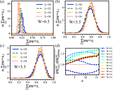
In Fig. 2 (a-c) we plot the probability distribution of IPR; here, we have calculated

$$\frac{1}{L}\sum_{\{\alpha\}}{\rm IPR}^{(\alpha)}$$ (36)

for different eigenstates $|\psi\rangle$ and for different disorder configurations, then considered its distribution as in the case of $P(\rho_{\alpha})$ in Sec. II B for different values of $W$ [(a) $W=0.5$, (b) $W=3.5$, (c) $W=5.5$]. The obtained $P(\sum{\rm IPR}/L)$ shows a sharply peaked distribution in the ETH phase [case (a)] peaked at a value $\propto 1/L$, while as $W$ increases, the center of the distribution is shifted to larger values; the peak also broadens in the regime of ETH-MBL transition. In the MBL phase the center of the distribution further approaches 1. A similar result has been reported in Fig. 3 of Ref. Bera et al., 2015. Thus, the real space character of the OPDM eigenvector, the natural orbitals $u^{(\alpha)}$ can be also used, together with the distribution of its eigenvalues, the occupation spectrum, to quantify the ETH-MBL transition.

We have repeated the same calculation in the basis of AL orbitals, and compared the results with those in the OPDM basis. Recall that AL orbitals are constructed in the non-interacting limit, while those of OPDM (natural orbitals) stem from an eigenstate of the full interacting system, and in this sense one can naturally assume that they represent dressed AL orbitals. The obtained $P(\sum{\rm IPR}/L)$ in the basis of AL orbitals shows features qualitatively similar to those in the OPDM basis, but still differs quantitatively, reflecting the effects of interaction in the natural orbitals. To highlight the difference, we plot in panel (d) the ratio of IPR in AL and OPDM bases; here, we have relabelled the eigenstates in the ascending order of IPR such that

$${\rm IPR}^{(\alpha_{1})}<{\rm IPR}^{(\alpha_{2})}<\cdots<{\rm IPR}^{(\alpha_{L})},$$ (37)

and consider the ratio: $\overline{{\rm IPR}^{(\alpha)}_{AL}}/\overline{{\rm IPR}^{(\alpha)}_{\rm OPDM}}$ at each $\alpha$, where $\overline{\cdots}$ represents sample averaging. In the regime of large $W$ (in the MBL phase) the above ratio shows a value superior to 1, typically for eigenstates with relatively small IPR; i.e., the natural orbitals are slightly more extended than AL orbitals. This is natural in the phenomenological LIOM picture, since LIOMs are considered to be dressed AL orbitals, while the natural orbitals are expected to mimic such LIOMs. The eigenstates with $\alpha\simeq\alpha_{L}$ showing IPR$\simeq 1$ are almost frozen and unaffected by the interaction; the above ratio is close to 1.

II.5 The multifractal dimension (IPR in Fock space)

To quantify the degree of localization in the Fock space more directly, we here consider, instead of Eq. (35), the IPR in the Fock space defined as

$${\cal IPR}_{\{n_{j}\}} = \sum_{\{n_{j}\}}\left|a_{\{n_{j}\}}\right|^{2q},$$ (38)

measuring to what extent a many-body eigenstate $|\psi\rangle$ spreads in the Fock space spanned by a many-body basis as given in Eq. (4). To demonstrate our numerical results we also employ a related quantity,

$$D_{q}=-\frac{\overline{\log{\cal IPR}_{\{n_{j}\}}}}{\log N},$$ (39)

called the multifractal dimension, where $N$ is the dimension of Hilbert space defined in Eq. (3). In the actual computation we consider the typical case of $q=2$. In Eq. (39), we have made explicit the specific way to take the ensemble average, since it may be more conventional to define $D_{q}$ such that

$$D_{q}=-\frac{\log\overline{{\cal IPR}_{\{n_{j}\}}}}{\log N},$$ (40)

while ${\cal IPR}_{\{n_{j}\}}$ is not self-averaging; i.e., $\overline{{\cal IPR}_{\{n_{j}\}}}$ does not converge rapidly.Solórzano et al. (2021) Here, to accelerate this convergence, we employ an alternative definition (39), in which we first take the logarithm of IPR_q to reduce the fluctuation, then sample average. Note that the logarithm of the IPR_q is often dubbed as participation Rényi entropy.

In Eq. (38) we have in mind that $|\psi\rangle$ is represented in the computational basis as in Eq. (2). In the ETH phase, the coefficients $a_{\{n_{j}\}}$’s are all on the same order; i.e., $|a_{\{n_{j}\}}|\simeq 1/\sqrt{N}$, so that IPR${}_{\{n_{j}\}}\sim 1/N$, or $D_{2}\simeq 1$, while we may a priori assume that IPR${}_{\{n_{j}\}}\simeq 1$ in the MBL phase (at the zeroth order) so that $D_{2}\simeq 0$. Hence, $D_{2}$ is presumed to show a jump: $1\rightarrow 0$ at the ETH-MBL transition. However, as pointed out in Refs. Macé et al., 2019; Tomasi et al., 2020, this is not precise; $D_{2}$ actually remains finite in the MBL phase. Here, we show through numerical simulations and the subsequent analytical considerations to what extent this remains finite depends, however, on the basis one employs for constructing the Fock space.

Using the OPDM creation operator (9), one can construct the many-body OPDM basis states:

$$|[\alpha]\rangle_{\rm OPDM} = c_{\alpha_{L/2}}^{\dagger}\cdots c_{\alpha_{2}}^{\dagger}c_{\alpha_{1}}^{\dagger}|0\rangle,$$ (41)

where the notation $[\alpha]$ has been introduced for distinguishing it from the full list $\{\alpha\}$. Unlike $\{\alpha\}$, $[\alpha]$ specify a selected list of states occupied in Eq. (41). In terms of these OPDM basis states we rewrite the many-body eigenstate $|\psi\rangle$ as

$$|\psi\rangle=\sum_{[\alpha]}a_{[\alpha]}|[\alpha]\rangle_{\rm OPDM}.$$ (42)

Using the coefficients $a_{[\alpha]}$ introduced above, we can define the Fock-space IPR in the OPDM basis as

$${\cal IPR}_{[\alpha]}=\sum_{[\alpha]}\left|a_{[\alpha]}\right|^{4}.$$ (43)

The coefficients $a_{[\alpha]}$ are computed from those in the computational basis [see Eq. (94)]. Similarly, one can define the Fock-space IPR in the AL orbital basis, employing in Eq. (43) the coefficients $a_{[\alpha]}^{(AL)}$ introduced in in Eq. (57) instead of the $a_{[\alpha]}$’s in Eq. (42). To find these coefficients $a_{[\alpha]}$ in the natural and AL orbital bases is numerically rather costly (see Appendix A).

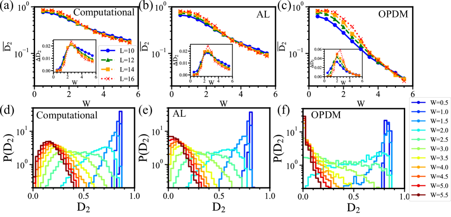
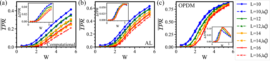
In Fig. 3 the fractal dimension $D_{2}$ has been computed (a) in the computational, (b) in the AL orbital, and (c) in the natural orbital (OPDM) bases, and its sample averaged values $\overline{D_{2}}$ are shown in the corresponding panels (a)-(c). The histograms (the probability distributions) of $D_{2}$ corresponding to the above three panels are shown in panels (d)-(f). Recall that $D_{2}$ is directly related to the Fock-space IPR (38) through the relation (39).

In the computational basis [panel (a) and (d)] one can confirm the characteristic behavior of $D_{2}$ in the ETH and MBL phases reported in Refs. Tomasi et al., 2020, i.e., $D_{2}\simeq 1$ in the ETH phase, while $D_{2}<1$ and fluctuates in the MBL phase. At $W\leq 1$ the histogram of $D_{2}$ shows a sharp peak at a value $\sim 0.8$ close 1. In the MBL regime: $W>3.5$, $D_{2}$ decreases but still takes a value $>10^{-1}$. The histogram of $D_{2}$ shows a broad maximum at a value approaching to 0 as $W$ increases.

In the OPDM basis [panel (c) and (f)] one can see that $D_{2}$ is clearly much suppressed ($<10^{-1}$) in the MBL regime [compare the MBL regime of panel (c) and that of panel (a); the order of $D_{2}$ differs; note the semi-log scale in the plots]. The shape of the histograms also differ in the MBL regime [panel (f) vs. panel (d)]. In panel (f), as $W$ increases, the distribution $P(D_{2})$ tends to be sharply peaked at $D_{2}=0$. In addition, the variance of $D_{2}$ shows a peak at the ETH-MBL transition much more enhanced in the OPDM basis; the height of the peak is three times larger ($\simeq 0.06$) than in other bases ($\Delta D_{2}\simeq 0.02$). At the transition $W\simeq 3$ the distribution $P(D_{2})$ becomes almost uniform, indicating that the multi-fractal dimension $D_{q}$ is actually non self-averaging.Tomasi et al. (2020); Solórzano et al. (2021) The finiteness of the Fock-space localization length is not only relevant to the finiteness of $D_{2}$ (i.e., $D_{2}\neq 0$) in the MBL phase but also to its behavior in the ETH-MBL crossover regime. These are part of the main findings in this work. Such peculiar behaviors of $\Delta D_{2}$ and $P(D_{2})$ at the putative ETH-MBL phase transition can be also seen away from the center of the spectrum: $\epsilon=0.5$, where

$$\epsilon=\frac{E-E_{min}}{E_{max}-E_{min}},$$ (44)

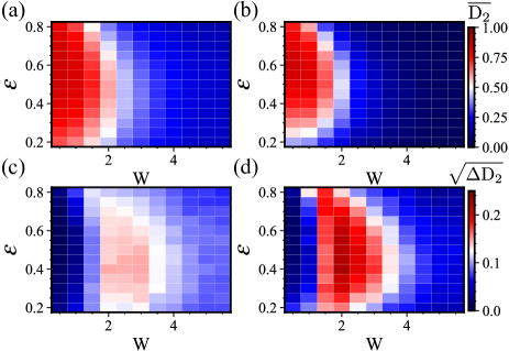
with $E_{min}$ and $E_{max}$ being respectively the minimum and maximum value of the eigenenergy $E$. In Appendix C, four panels of Fig. 8 show ETH-MBL phase diagrams determined by the calculated values of $D_{2}$ and its fluctuation. In the OPDM basis [panel (b)] sharply contrasting values of $D_{2}$ are found in the ETH and MBL phases, subsutantially improving the quality of the phase diagram as compared to the one in the computational basis [panel (a)]. In panel (d) the fluctuation $\Delta D_{2}$ shows a conspicuous peak in the ETH-MBL crossover regime, a behavior consistent with Fig. 3 (f); see Appendix C for details. Results in the AL orbital basis [panel (b) and (e)] show features intermediate between the OPDM and the computational bases.

Such a conspicuous suppression of $D_{2}$ in the MBL regime under the OPDM basis confirms that the natural orbitals are indeed good approximation of the LIOM orbitals. We have previously argued that under the assumption that only the first term of LIOM creation operator (20) is relevant, and the higher order terms are negligible, the natural orbitals $u_{\alpha}$ coincide with the LIOM orbitals. We then hypothesized that in a generic MBL situation this assumption approximately holds, leading to a consistent description of the behavior of the occupation spectrum and its probability distribution. Here, the behavior of multifractal dimension $D_{2}$ confirms this hypothesis.

In terms of the LIOM creation operators $\gamma_{\alpha}^{\dagger}$, a many-body eigenstate $|\psi\rangle$ can be written in the simple product form as in Eq. (17). This means that if $|\psi\rangle$ is represented in the (hypothetical) LIOM basis as

$$|\psi\rangle=\sum_{[\beta]}a_{[\beta]}|[\beta]\rangle_{\rm LIOM},$$ (45)

then a single component $a_{[\beta_{0}]}=1$ is finite, and others vanish: $a_{[\alpha\neq\beta_{0}]}=0$. The resulting ${\cal IPR}_{[\beta]}$ in this idealized LIOM basis is strictly 1, and the corresponding $D_{2}$ strictly vanishes, implying that in this case a ultimately restricted part of the total Hilbert space is available for the realized eigenstates. In a generic interacting many-body eigenstate $|\psi\rangle$, such (i.e., $D_{2}=0$) usually does not happen, and is unique to the case in which $|\psi\rangle$ is expressed as in Eq. (17) in a simple product form.

In the computational basis the same $|\psi\rangle$ is expressed as in Eq. (2), or here we rather express it as

$$|\psi\rangle=\sum_{[j]}a_{[j]}|[j]\rangle,$$ (46)

where for specifying a basis in the computational basis we have employed, instead of Eq. (4), an alternative notation:

$$|[j]\rangle=c_{j_{L/2}}^{\dagger}\cdots c_{j_{2}}^{\dagger}c_{j_{1}}^{\dagger}|0\rangle.$$ (47)

Then, the coefficient $a_{[j]}$ is given a simple expression:

$$a_{[j]} = \langle[j]|[\beta_{0}]\rangle_{\rm LIOM},$$ (48)

where $\langle[j]|[\beta]\rangle_{\rm LIOM}$ is given by the following Slater determinant:

$$\langle[j]|[\beta]\rangle_{\rm LIOM} = \det\left[\begin{array}[]{cccc}A^{(\beta_{1})}_{j_{1}}&A^{(\beta_{2})}_{j_{1}}&\cdots&A^{(\beta_{L/2})}_{j_{1}}\\ A^{(\beta_{1})}_{j_{2}}&A^{(\beta_{2})}_{j_{2}}&\cdots&A^{(\beta_{L/2})}_{j_{2}}\\ \vdots&\vdots&&\vdots\\ A^{(\beta_{1})}_{j_{L/2}}&A^{(\beta_{2})}_{j_{L/2}}&\cdots&A^{(\beta_{L/2})}_{j_{L/2}}\end{array}\right]$$ (53)

of LIOM orbitals $A^{(\beta)}_{j}$, which is assumed to behave as in Eq. (29); i.e., Then, among the coefficients $a_{[j]}$’s in Eq. (48) the dominant contribution is from $[j]=[j_{0}]$ such that all the $j$’s in $[j_{0}]$ coincide with one of the localization centers $j_{\beta}$ of an occupied state in $|[\beta_{0}]\rangle_{\rm LIOM}$ [see Eq. (29)], and is found to be

$$a_{[j_{0}]} = \langle[j]|[\beta_{0}]\rangle_{\rm LIOM}\simeq\prod_{\beta\in[\beta_{0}]}A^{(\beta)}_{j_{\beta}}$$ (54)

$$\simeq \prod_{\beta\in[\beta_{0}]}\sqrt{\tanh\frac{1}{2\xi_{\beta}}}\equiv\left(\tanh\frac{1}{2\overline{\xi}}\right)^{L/4},$$

where in the estimation of the determinants (53), we have kept only the dominant contribution from the diagonal terms $A^{(\beta_{j})}_{j}$, while in the last step we have introduced the typical localization length $\overline{\xi}$. The coefficients $a_{[j]}$ in the computational basis is distributed around the single site ${[j_{0}]}$ in the Fock space. At the leading order, $a_{[j]}$ has contributions from “sites” ${[j^{\prime}]}$ such that one of the $j$’s in $[j^{\prime}]$ is found to be in a neighboring site of a localization center $j_{\beta}$, while others coincide with one of the remaining $j_{\beta}$’s of an occupied state. The contribution from such sites ${[j^{\prime}]}$ is on the order of

$$a_{[j^{\prime}]}\simeq e^{-1/(2\overline{\xi})},$$ (55)

and there are order $L$ of such sites. As for contributions to IPR, the dominant correction to the ideal value 1 is from the correction given in (54), and the correction from $a_{[j^{\prime}]}$ gives only a subdominant contribution; i.e.,

$$IPR \simeq |a_{[j_{0}]}|^{4}+L|a_{[j^{\prime}]}|^{4}+\cdots$$ (56)

$$\simeq \left(\tanh\frac{1}{2\overline{\xi}}\right)^{L}+Le^{-1/(2\overline{\xi})}+\cdots.$$

We have checked the validity of the formulas (54), (55) and (56) numerically [see Appendix B]. This, in turn, at least indirectly certifies the validity of our hypothesis that the many-body eigenstate $|\psi\rangle$ can be expressed as a simple product of LIOM orbitals as in Eq. (17), and of the subsequent assumptions on LIOMs.

In the AL orbital basis, one expresses $|\psi\rangle$, instead of Eq. (46), as

$$|\psi\rangle=\sum_{[\alpha]}a_{[\alpha]}^{(AL)}|[\alpha]\rangle_{AL}.$$ (57)

where $|[\alpha]\rangle_{AL}$ represents the AL orbital basis:

$$|[\alpha]\rangle_{AL} = c_{AL}^{(\alpha_{L/2})\dagger}\cdots c_{AL}^{(\alpha_{2})\dagger}c_{AL}^{(\alpha_{1})\dagger}|0\rangle,$$ (58)

while the AL orbital creation operator $c_{AL}^{(\alpha)\dagger}$ has been defined in Eq. (27). The coefficients $a_{[\alpha]}^{(AL)}$ in Eq. (57) are given a simple expression:

$$a_{[\alpha]}^{(AL)} = \ {}_{AL}\langle[\alpha]|[\beta_{0}]\rangle_{\rm LIOM},$$ (59)

where the unitary transformation $\langle[\alpha]|[\beta]\rangle_{\rm LIOM}$ is given by the following determinant:

$$\ {}_{AL}\langle[\alpha]|[\beta]\rangle_{\rm LIOM} = \det\left[\begin{array}[]{cccc}\tilde{A}^{(\beta_{1})}_{\alpha_{1}}&\tilde{A}^{(\beta_{2})}_{\alpha_{1}}&\cdots&\tilde{A}^{(\beta_{L/2})}_{\alpha_{1}}\\ \tilde{A}^{(\beta_{1})}_{\alpha_{2}}&\tilde{A}^{(\beta_{2})}_{\alpha_{2}}&\cdots&\tilde{A}^{(\beta_{L/2})}_{\alpha_{2}}\\ \vdots&\vdots&&\vdots\\ \tilde{A}^{(\beta_{1})}_{\alpha_{L/2}}&\tilde{A}^{(\beta_{2})}_{\alpha_{L/2}}&\cdots&\tilde{A}^{(\beta_{L/2})}_{\alpha_{L/2}}\end{array}\right]$$ (64)

of $\tilde{A}^{(\beta)}_{\alpha}$ given in Eq. (31), representing physically the overlap of the $\alpha$th AL orbital and $\beta$th LIOM orbital. Unlike in the computational basis, in which this overlap becomes each component of the LIOM wave function $A^{(\beta)}_{j}$, here $\tilde{A}^{(\beta)}_{\alpha}$ in Eq. (64) represents the overlap (31), which becomes on the diagonal terms of Eq. (64)

$$\tilde{A}^{(\beta)}_{\beta}=\sum_{j}\psi_{AL}^{(\beta)*}(j)A^{(\beta)}_{j},$$ (65)

and takes a value close to 1; at least, a value closer to 1 than the simple peak value:

$$A^{(\beta)}_{j_{\beta}}\simeq\sqrt{\tanh\left(\frac{1}{2\xi_{\beta}}\right)}.$$ (66)

One can check this hypothesis by assuming the following explicit form for the AL orbitals:

$$\psi_{\alpha}^{(AL)}(j)=\sqrt{\tanh\frac{1}{2\xi_{\alpha}^{(AL)}}}\exp\left(-\frac{|j-j_{\alpha}|}{2\xi_{\alpha}^{(AL)}}\right).$$ (67)

Then, one finds that the inequality $\tilde{A}^{(\beta)}_{\beta}>A^{(\beta)}_{j_{\beta}}$ holds for a relatively broad range of $\xi_{\alpha}^{(AL)}$. As a result, ${\cal IPR}_{[\alpha]}^{(AL)}$ in the AL orbital basis dominated by the term:

$$a_{[\beta_{0}]}^{(AL)} = \ {}_{AL}\langle[\beta_{0}]|[\beta_{0}]\rangle_{\rm LIOM}\simeq\prod_{\beta\in[\beta_{0}]}\tilde{A}^{(\beta)}_{\beta},$$ (68)

takes a value much closer to 1 than in the computational basis, and the corresponding $D_{2}$ is more suppressed in the MBL phase. In the OPDM basis, this tendency is further accentuated: ${\cal IPR}_{[\alpha]}\simeq 1$, and the corresponding $D_{2}$ practically vanishes. These results confirm that the OPDM basis is closest to LIOM orbitals; AL orbitals are less appropriate approximation of them, while the effect of a finite spread of LIOM orbitals in real space [see Eq. (29)] is most visible in the Fock-space IPR represented in the computational basis.

This observation on the practical vanishing of $D_{2}\simeq 0$ in the Fock space (under the OPDM basis and in the MBL phase) is consistent with the behavior of the gapped occupation spectrum $\{\rho_{\alpha}\}$ and the corresponding V-shaped probability distribution $P(\rho_{\alpha})$ we have described in Secs. II A and C. In the deep MBL phase, the eigenstate is predominantly expressed by a product state (17) of LIOM $\simeq$ OPDM orbitals, in which the occupation spectrum $\rho_{\alpha}$ in principle coincides with the occupation number $n_{\alpha}=0,1$ specifying the basis state $|[\beta_{0}]\rangle_{\rm LIOM}$; $n_{\alpha}=1$ ($n_{\alpha}=0$) represents simply the occupation (vacancy) of the $\alpha$th orbital. The resulting probability distribution $P(\rho_{\alpha})$ tends to become bimodal; this tendency has been seen in the V-shaped distribution in Fig. 3 (f). The occupation spectrum in the computational basis is, on the other hand, directly susceptible of a finite spread of LIOM orbitals in real space [see Eq. (29)]; as a result the jump of the occupation spectrum tends to be washed out, and the corresponding probability distribution becomes U-shaped [Fig. 3 (d)]. In the AL orbital basis, we have seen features intermediate of the above two cases.

In Ref. Tomasi et al., 2020 it has been pointed out that the multifractal dimension of an eigenstate constructed from a single Slater determinant remains finite and fluctuates, even in the localized phase. This is very much consistent with what we have described above in the case of computational basis, and here it has been more thoroughly analyzed from the scope of our study on the basis dependence of the multifractal dimension behavior.

In reality, on the other hand, one cannot fully escape from thermal region effects; i.e., higher-order terms in the LIOM creation operator (20) introduce particle-hole excitations to the product state (17), transforming it to a superposition state; i.e., entanglement is generated. In real space this appears as thermal regions, while in Fock space more states become available for realized eigenstates. In the next section, we focus on the quantity dubbed as the local purity and shed light on the relation between the occupation spectrum and the multifractal dimension.

The comparison of Eqs. (38) and Eqs. (43) has been done in Ref. Buijsman et al., 2018, and it was found that the coefficients $a_{\{\alpha\}}$ in the OPDM basis are more localized in the MBL phase than $a_{\{n_{j}\}}$ in the computational basis; i.e., IPR_{α} is closer to 1 than IPR${}_{\{n_{j}\}}$ in the MBL phase; to be precise the authors of Ref. Buijsman et al., 2018 compared the participation ratio ($=1/$IPR) in the computational and in the OPDM bases [see two panels of Fig. 2 in Ref. Buijsman et al., 2018].

We have typically sampled $10^{1}-10^{2}$ eigenstates for each disorder realization, and the number of disorder realizations are $2\times 10^{2}(W\leq 2.5,L=16)-10^{3}$. The total number of samples in the OPDM basis is more than $10^{4}$ for $L\leq 14$ and $2\times 10^{3}(W\leq 2.5)-5\times 10^{3}(W\geq 3.0)$ for $L=16$. This is $2-5$ times more than those of Ref. Buijsman et al., 2018, and obtained results are consistent with those of Ref. Buijsman et al., 2018.

Figure 4: The ensemble average of the local purity $\overline{S}$ evaluated in different many-body bases: (a) the computational basis, (b) the AL orbital basis, and (c) natural orbital (OPDM) basis, at different strength $W$ of disorder. In the curves represented by solid lines $S$ is evaluated in its full form [as in Eq. (69), or in Eq. (80)], while in those represented by dashed lines in an approximate form [as given in the second line of Eq. (89)]. The insets show its variance $\Delta S$.

III Local purity and its moments, Hamming distance

III.1 From occupation spectrum to local purity

The degree of Fock-space localization is also encoded in how close the occupation spectrum $\rho_{\alpha}$ is to a simple step function (16). Here, to quantify this we employ the quantity, referred to as the local purity in Ref. Viola and Brown, 2007. The local purity $S$ of a many-body state $|\psi\rangle$ is defined as

$$S=\frac{1}{L}\sum_{\alpha=\alpha_{1}}^{\alpha_{L}}\langle\psi|\hat{\sigma}_{{\alpha}}|\psi\rangle^{2},$$ (69)

where

$$\hat{\sigma}_{\alpha}=2\hat{n}_{\alpha}-1=2c_{\alpha}^{\dagger}c_{\alpha}-1$$ (70)

measures how the occupation of $j$th orbital $\langle\hat{n}_{\alpha}\rangle=\langle\psi|\hat{n}_{\alpha}|\psi\rangle$ deviates from 1/2; i.e., $\langle\hat{\sigma}_{\alpha}\rangle=1$ if $\langle\hat{n}_{\alpha}\rangle=1$ while $\langle\hat{\sigma}_{\alpha}\rangle=-1$ if $\langle\hat{n}_{\alpha}\rangle=0$. In a maximally localized MBL state and if ${\alpha}_{j}$’s are chosen to be LIOM orbitals, then $S=1$, while in the ETH phase $\langle\hat{n}_{\alpha}\rangle\simeq 1/2$ so that $S\simeq 0$. Here, we have in mind a situation in which the state $|\psi\rangle$ is expressed as a superposition of many-body basis states $|\mu\rangle$ as

$$|\psi\rangle=\sum_{\mu}a_{\mu}|\mu\rangle,$$ (71)

where $\mu$ is, e.g., specified by a Fock representation:

$$\mu=\{n_{\alpha}\}=(n_{\alpha_{1}},n_{\alpha_{2}},\cdots,n_{\alpha_{L}}).$$ (72)

The integers $n_{\alpha}=0,1$ specify how many electrons are in the state $\alpha$ ($\alpha$th orbital) in the basis state $|\mu\rangle$. For basis orbitals $\alpha$’s we consider the specific cases of natural (OPDM) and AL orbitals as concrete examples. In the case of computational basis a basis state $|\mu\rangle$ specified by Eq. (72) reduces to Eq. (4). Note that in the new notation $\mu$ we label a many-body basis state such as the ones given in Eqs. (4), (41), or (58) by a single label $\mu$, which is later specified by a single number: $\mu=0,1,2,\cdots,N-1$. Note also that the choice of our operator $\hat{\sigma}_{\alpha}$ in Eq. (70) is basis dependent, and chosen in such a way that $\hat{\sigma}_{\alpha}$ is a good quantum number for a basis state $|\mu\rangle$; i.e., $\hat{\sigma}_{\alpha}=+1$ if $n_{\alpha}=1$ in $\mu$, while $\hat{\sigma}_{\alpha}=-1$ if $n_{\alpha}=0$ in $\mu$. Thus, the contribution of a basis state $|\mu\rangle$ to the quantity $\langle\hat{\sigma}_{\alpha}\rangle=\langle\psi|\hat{\sigma}_{\alpha}|\psi\rangle$ is either $+1$ if $n_{\alpha}=1$ in $\mu$, or $-1$ if $n_{\alpha}=0$ in $\mu$. Based on these two types of contributions to $\langle\hat{\sigma}_{\alpha}\rangle$, let us classify the set of $N$ basis states $\{\mu\}$ into two categories: $\{\alpha_{\uparrow}\}$ and $\{\alpha_{\downarrow}\}$, where $\mu\in\{\alpha_{\uparrow}\}$ if $n_{\alpha}$ in Eq. (72) is $+1$, while $\mu\in\{\alpha_{\downarrow}\}$ if $n_{\alpha}$ in Eq. (72) is $-1$. This allows us to express $\langle\hat{\sigma}_{\alpha}\rangle$ as

$$\langle\hat{\sigma}_{\alpha}\rangle = \langle\psi|\hat{\sigma}_{\alpha}|\psi\rangle$$ (73)

$$= \left(\sum_{\mu\in\{\alpha_{\uparrow}\}}-\sum_{\mu\in\{\alpha_{\downarrow}\}}\right)|a_{\mu}|^{2}$$

Substituting Eq. (73) into the definition of the local purity (69), one can prove Viola and Brown (2007) (see Appendix B),

$$S = \frac{1}{L}\sum_{\alpha=\alpha_{1}}^{\alpha_{L}}\langle\hat{\sigma}_{\alpha}\rangle^{2}$$ (74)

$$= 1-\frac{4}{L}\sum_{\mu<\nu}x_{\mu\nu}|a_{\mu}|^{2}|a_{\nu}|^{2},$$

where $x_{\mu\nu}$ represents the Hamming distance between the two basis states $|\mu\rangle$ and $|\nu\rangle$. In the last step to find the final expression for the purity in Eq. (74) we have noted the following identity:

$$\sum_{\alpha=\alpha_{1}}^{\alpha_{L}}\sum_{\mu\in\{\alpha_{\uparrow}\}}\sum_{\nu\in\{\alpha_{\downarrow}\}}|a_{\mu}|^{2}|a_{\nu}|^{2}=\sum_{\mu<\nu}x_{\mu\nu}|a_{\mu}|^{2}|a_{\nu}|^{2}$$ (75)

where $\sum_{\mu\in\{\alpha_{\uparrow}\}}$, $\sum_{\nu\in\{\alpha_{\downarrow}\}}$, or rather the underlying classification of the states $|\mu\rangle$ into $\{\alpha_{\uparrow}\}$ and $\{\alpha_{\downarrow}\}$ is (implicitly) dependent on $j$, since at each $j$ we have classified $|\mu\rangle$ based on the value of $n_{\alpha}$ in $|\mu\rangle$. To verify Eq. (75) let us consider how many times a given combination $|a_{\mu}|^{2}|a_{\nu}|^{2}$ appears in the summation on the l.h.s. of Eq. (75). Provided that $\mu\neq\nu$, $n_{\alpha}$’s in $\mu$ and $\nu$ differ at least some $\alpha$, and at this $\alpha\equiv\tilde{\alpha}_{1}$ either $\mu\in\{\alpha_{\uparrow}\}$ and $\nu\in\{\alpha_{\downarrow}\}$ or vice versa holds; i.e., at this $\alpha$ the combination $|a_{\mu}|^{2}|a_{\nu}|^{2}$ is eligible for being included in the summation on the l.h.s. of Eq. (75), i.e., in $\sum_{\mu\in\{\alpha_{\uparrow}\}}\sum_{\nu\in\{\alpha_{\downarrow}\}}|a_{\mu}|^{2}|a_{\nu}|^{2}$. If $n_{\alpha}$’s in $\mu$ and $\nu$ also differ at some another $\alpha=\tilde{\alpha}_{2}$, then at this value of $\alpha=\tilde{\alpha}_{2}$ the combination $|a_{\mu}|^{2}|a_{\nu}|^{2}$ is again eligible for being included in the same summation; and the same may happen again at $\alpha=\tilde{\alpha}_{3}$, etc. Thus, the combination $|a_{\mu}|^{2}|a_{\nu}|^{2}$ appears on the l.h.s. of Eq. (75) $x_{\mu\nu}$ times, where $x_{\mu\nu}$ is the number of times in which $n_{\alpha}$’s in $\mu$ and $\nu$ differ, and this number $x_{\mu\nu}$, measuring the distance in Fock space between the two states $|\mu\rangle$ and $|\nu\rangle$ is often referred to as Hamming distance. Tomasi et al. (2020); Roy et al. (2019); Roy and Logan (2020)

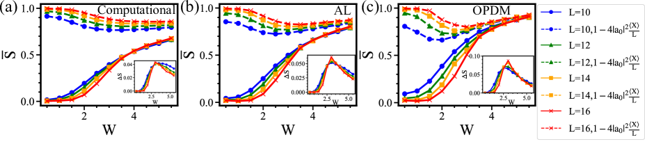
In Fig. 4, the purity $S$ evaluated in the three different many-body bases; (a) computational, (b) AL orbital, and (c) natural orbital (OPDM) bases. is shown as a function of $W$ and compared. In the three bases, one can see the expected tendencies: i.e., the purity $S$ tends to vanish in the ETH phase: $S\simeq 0$ as $L$ increase, while in the MBL phase $S$ takes a value on the order of unity. Thus, in the limit of large $L$, as $W$ increases, the value $S=0$ in the ETH phase is expected to jump into a finite value at the ETH-MBL transition: $W\simeq 3.5-4$, while the magnitude of this jump $\delta S$ is largest (smallest) in the OPDM (computational) basis. As $W$ is further increased, the value of $S$ tends to approach the ideal value 1 in the OPDM basis, while in the computational basis it remains to be a value considerably smaller than 1. In the AL orbital basis, features intermediate between the two cases are seen.

In the computational basis the deviation of $S$ from the ideal value 1 has two independent sources. One is the imperfection of the Fock-space localization in the MBL phase due to higher-order terms in Eq. (20); i.e., the effect of thermal regions, while the other is the finite localization length; i.e., a finite spread of the hypothetical LIOM wave functions in real space [cf. Eq. (29)]. We have previously seen that in the computational basis one is strongly susceptible of the second effect; cf. discussion on the multifractal dimension in the computational basis (Sec. II-E). On the other hand, in the OPDM basis, one is almost free from this extrinsic effect (second effect). Therefore, the remaining deviation of $S$ in the MBL phase from the ideal value 1 in the OPDM basis quantifies the degree of intrinsic imperfection of the Fock-space localization due to the presence of thermal regions, and the finiteness of the jump $\Delta S$ is possibly related to the KT nature of the ETH-MBL transition.

Figure 5: The distribution $\Omega_{x}$ [see Eq. (77)] of the Hamming distance $x$ computed in the different many-body bases: (a) computational, (b) AL orbital, and (c) natural orbital (OPDM).

III.2 Purity vs. Fock-space IPR

Let us compare the expression (74) for the local purity with the one for IPR in Fock space:

$${\cal IPR} = \sum_{\mu}|a_{\mu}|^{4}$$ (76)

$$= 1-2\sum_{\mu<\nu}|a_{\mu}|^{2}|a_{\nu}|^{2}.$$

In the second line, ${\cal IPR}$ has been rewritten in a form similar to Eq. (74); see Appendix C for its derivation. The local purity $S$ and ${\cal IPR}$ are similar quantities, both measuring the degree of Fock-space localization, taking values $\simeq 1$ in the MBL (Fock-space localized) phase, while $\simeq 0$ in the ETH (Fock-space delocalized) phase. Comparing Eqs. (74) and (76), one can see that the two quantities, indeed follow a similar expression, except one remarkable difference; in the sum collecting the contributions from pairwise amplitudes $|a_{\mu}|^{2}|a_{\nu}|^{2}$, each contribution is weighted in Eq. (74) by the Hamming distance $x_{\mu\nu}$ between the two basis states between $|\mu\rangle$ and $|\nu\rangle$, while it is not in Eq. (76).

To quantify the contributions from different Hamming distance pairs let us introduce the quantity:

$$\Omega_{x}=\sum_{\mu<\nu s.t.x_{\mu\nu}=x}|a_{\mu}|^{2}|a_{\nu}|^{2},$$ (77)

where the summation is for all pairs $\mu<\nu$ such that their Hamming distance $x_{\mu\nu}$ is constrained to a specific value $x=1,2,\cdots$. For $x=0$, let us define $\Omega_{0}$ such that

$$\Omega_{0}=\sum_{\mu}|a_{\mu}|^{4}={\cal IPR}_{\{a_{\mu}\}}$$ (78)

Using $\Omega_{x}$, one can reexpress the second term of Eq. (74) as

$$\sum_{\mu<\nu}x_{\mu\nu}|a_{\mu}|^{2}|a_{\nu}|^{2} = \sum_{x}x\sum_{\mu<\nu s.t.x_{\mu\nu}=x}|a_{\mu}|^{2}|a_{\nu}|^{2}$$ (79)

$$= \sum_{x=1}^{\infty}x\Omega_{x},$$

i.e.,

$$S = 1-\frac{4}{L}\sum_{x=1}^{\infty}x\Omega_{x}.$$ (80)

Using $\Omega_{x}$, one can also rewrite Eq. (38) as

$${\cal IPR} = 1-2\sum_{x=1}^{\infty}\Omega_{x}.$$ (81)

The form of Eqs. (80) and (81) suggests that $\Omega_{x}$ plays the role of a probability distribution for $x$. It indeed is for the occurrence of a pair $c_{\alpha_{\mu}}^{\dagger}$ and $c_{\alpha_{\nu}}^{\dagger}$ in the given many-body (eigen)states $|\psi\rangle$. Also, the summation in Eqs. (80) and (81) starts from $x=1$ in the generic case, while in our present context with a fixed electron density (to $\nu=1/2$), the summation actually starts from 2, and $x$ takes only even integer values provided that $L$ is even.

In three panels of Fig. 5 the pairwise distribution $\Omega_{x}$ computed under different bases has been ensemble averaged and plotted against the Hamming distance $x$. The plots show the evolution of the distribution $\Omega_{x}$ as a function of $W$. At weak $W$; i.e. in the ETH phase, the distribution $\Omega_{x}$ shows a broad maximum around the center of the Fock-space hypercube $x\simeq L/2$, while as $W$ increases, the center of mass of the distribution gradually shifts to $x=0$, and in the MBL phase $\Omega_{x}$ becomes maximal at $x=0$. In the OPDM basis [panel (c)] $\Omega_{x}$ is sharply peaked at $x=0$; the peak is sharp and high: $\Omega_{0}\simeq 0.8$, while in the computational basis [panel (a)] $\Omega_{x}$ exhibits a relatively long tail that extends almost as far as $x=L/2$. In the AL orbital basis the behavior of $\Omega_{x}$ is intermediate between the two cases.

The height of the peak at $x=0$ is $\Omega_{0}$ [see Eq. (78)], which is nothing but the value of Fock-space IPR discussed in the previous section. In the computational basis [panel (a)] the Fock-space IPR is, as was also the case in the local purity $S$, strongly susceptible of the finite localization length; i.e., a finite spread of the hypothetical LIOM wave functions in real space [cf. Eq. (29) and Eqs. (54), (55), (56)]. Note that the peak of the LIOM wave function diminishes since it spreads; diminishes to compensate for the normalization, giving the principal reason why $\Omega_{0}$ is relatively small in panel (a). In the OPDM basis [panel (c)], on the other hand, this extrinsic effect is almost removed so that the peak height $\Omega_{0}$ is close to the ideal value 1 in the deep MBL regime. To quantify the behavior of $\Omega_{x}$ in a broader regime of $W$, let us further analyze the nature of this quantity in the next subsection.

Figure 6: Comparison of the total Fock-space IPR and the contribution from $|a_{0}|^{4}$ [cf. Eq. (90)] (a) in the computational, (b) in the AL orbital, and (c) in the natural orbital (OPDM) bases. The insets show the variance $\Delta{\cal IPR}$.

III.3 $\Omega_{x}$ vs. $\Pi(x)$

In the MBL phase the state $|\psi\rangle$ is close to a simple product state such as the one given in Eq. (17); i.e., in the superposition of Eq. (71), the contribution from a single component $\mu=\mu_{0}$ predominates, and those from other basis states $\mu\neq\mu_{0}$ are minor. To make clear the situation, let us relabel $\mu$’s such that

$$|a_{0}|>|a_{1}|>|a_{2}|>\cdots,$$ (82)

then one can naturally assume that

$$|a_{0}|\gg|a_{1}|,|a_{2}|,\cdots.$$ (83)

In Fig. 5 (c) the value of $\Omega_{0}$ [cf. Eq. (78)] is closest to 1 in panel (c); i.e., in the OPDM basis: $\Omega_{0}=|a_{0}|^{4}\simeq 0.8$ in the deep MBL regime, so that $|a_{0}|^{2}$ will be even closer to 1. Therefore, $|a_{0}|^{2}\gg$ all other $a_{\mu}$’s. The inequality (83) signifies that among the contribution from various pairs $|a_{\mu}|^{2}|a_{\nu}|^{2}$ in Eq. (77) only terms containing $|a_{0}|^{2}$ give principal contributions, i.e., Eq. (77) can be well-approximated as

$$\Omega_{x} = \sum_{\mu<\nu s.t.x_{\mu\nu}=x}|a_{\mu}|^{2}|a_{\nu}|^{2}$$ (84)

$$\simeq |a_{0}|^{2}\sum_{\mu{\rm s.t.}x_{\mu,0}=x}|a_{\mu}|^{2}\equiv|a_{0}|^{2}\Pi(x).$$

In the last line we have introduced the quantity

$$\Pi(x)=\sum_{\mu{\rm s.t.}x_{\mu,0}=x}|a_{\mu}|^{2},$$ (85)

which has been dubbed as radial distribution in Ref. Tomasi et al., 2020. As a distribution, this quantity $\Pi(x)$ may be better behaved than our $\Omega_{x}$ given in Eq. (77) in the sense that with a natural convention of $\Pi(0)=|a_{0}|^{2}$, $\Pi(x)$ has been automatically normalized:

$$\sum_{x=0}^{\infty}\Pi(x) = \sum_{x=0}^{\infty}\sum_{\mu{\rm s.t.}x_{\mu,0}=x}|a_{\mu}|^{2}=\sum_{\mu}|a_{\mu}|^{2}=1.$$ (86)

The radial distribution $\Pi(x)$ measures the Hamming distance $x$ from a principal component $|\mu_{0}\rangle$, while the distribution $\Omega_{x}$ measures its occurrence in the entire distribution of basis states $|\mu\rangle$. In the light of Eq. (84) let us further interpret the results shown in Fig. 5. We have previously considered the case in which $W$ is strong enough for the system to be in the deep MBL limit, where the many-body eigenstate $|\psi\rangle$ is expressed by a simple product state as in Eq. (17), then $\Omega_{x}$ is sharply peaked at $x=0$. This is typically the case in panel (c) in the OPDM basis, since the natural orbitals $\simeq$ LIOMs, and in the OPDM basis $|\psi\rangle$ may still be well approximated by the simple product state:

$$|\psi\rangle\simeq c_{\beta_{L/2}}^{\dagger}\cdots c_{\beta_{2}}^{\dagger}c_{\beta_{1}}^{\dagger}|0\rangle\equiv|[\beta_{0}]\rangle_{\rm OPDM},$$ (87)

where $c_{\beta}^{\dagger}$ creates an electron in the $\beta$th natural orbital. As $W$ decreases, however, higher-order terms of LIOM; i.e., such as the $B$-terms in Eq. (20) become non-negligible, and add to the principal product state (87) those terms that can be created by particle-hole excitations; i.e.,

$$|\psi\rangle\simeq\left[1+\sum_{\alpha\beta}\tilde{B}_{\alpha\beta}c_{\alpha}^{\dagger}c_{\beta}+\cdots\right]|[\beta_{0}]\rangle_{\rm OPDM},$$ (88)

where the second and higher-order terms create states that are detached from $|[\beta_{0}]\rangle_{\rm OPDM}$ in Fock space by the Hamming distance $x$ equal to twice the number of particle-hole excitations. As $W$ decreases and the system approaches the MBL-ETH transition, such higher-order terms tend to become more important. As a result, the state $|\psi\rangle$ initially point-localized in the Fock space at $[\beta]=[\beta_{0}]$ acquires a finite expanse specified by the distribution $\Omega_{x}$. In panels (c) and (b) of Fig. 5 the distribution $\Omega_{x}$ is sharply peaked at $x=0$ in the deep MBL phase, while as $W$ decreases it resolves itself into a broader distribution extended to the region of $x\neq 0$. Such an evolution is well explained by the appearance of higher-order terms in Eq. (88) that physically represent particle-hole excitations. How much weight the distribution $\Omega_{x}$ has away from $x=0$ is a measure of to what degree such states created by particle-hole excitations are mixed with the principal product state $|[\beta_{0}]\rangle_{\rm OPDM}$ in the realized eigenstate $|\psi\rangle$.

In terms of $\Pi(x)$ and in the MBL phase Eq. (80) may be rewritten as

$$S = 1-\frac{4}{L}\sum_{x=1}^{\infty}x\Omega_{x}$$ (89)

$$\simeq 1-\frac{4}{L}|a_{0}|^{2}\sum_{x=1}^{\infty}x\Pi(x).$$

In Fig. 4 the purity $S$ is evaluated both in its full [as in the first line of Eq. 89)] and asymptotic [as in the second line of Eq. 89)] forms, and they are plotted together for comparison in the three different bases: (a) computational, (b) AL orbital, and (c) natural orbital (OPDM). The two quantities tend to merge in the MBL phase in the three bases, but the agreement is best and almost perfect in the OPDM basis and in the deep MBL regime. Note that the two quantities coincide signifies that the principal component $a_{0}$ is indeed predominant, and the assumption (83) is well justified. The fact that $S$ deviates significantly from its asymptotic expression [the second line of Eq. 89)] signifies that the quantity $S$ well describes the expanse the weight of $|\psi\rangle$ on $a_{\mu}$ around $a_{0}$.

Using $\Omega_{x}$, one can also rewrite Eq. (81) as

$${\cal IPR} = 1-2\sum_{x=1}^{\infty}\Omega_{x}$$ (90)

$$\simeq 1-2|a_{0}|^{2}\sum_{x=1}^{\infty}\Pi(x)$$

$$= 1-2|a_{0}|^{2}+2|a_{0}|^{4}\geq|a_{0}|^{4}.$$

In Fig. 6 the total Fock-space IPR and the contribution from $|a_{0}|^{4}$ (cf. the last expression above) have been plotted together and compared in the three different bases: (a) computational, (b) AL orbital, and (c) natural orbital (OPDM). The plots show that actually in all the bases and in all range of $W$, the two quantities almost coincide; i.e., $|a_{0}|^{4}$ is a good approximation of the Fock-space IPR, and the agreement is almost perfect in the OPDM basis. This, in turn, implies that unlike the local purity $S$ in Fig. 4 the Fock-space IPR is almost exclusively determined by the principal term $a_{0}$ and not much sensitive to the expanse of the weight of $|\psi\rangle$ in the Fock space around $a_{0}$.

IV Concluding remarks

To highlight the nature of many-body localization (MBL), especially focusing on its aspect of Fock-space localization, we have considered a paradigmatic model of MBL; a one-dimension spinless fermion model (1). As a practical tool of the analysis we have employed the one-particle density matrix (OPDM) approach [see Eq. (6)]. The natural orbitals, i.e., the eigenvectors of the OPDM are expected to mimic the local integrals of motion (LIOMs) emergent in the MBL phase. We have thus expected that the use of natural orbitals as basis states (i.e., the use of OPDM basis), minimizing effects of the finiteness of Fock-space localization length, qualitatively improves our description of the ETH-MBL crossover regime.

We begin by investigating the occupation spectrum $\rho_{\alpha}$ (the eigenvalues of OPDM) and the natural orbitals as a measure for quantifying the degree of Fock-space localization prevailing in the system. In the MBL phase, $\rho_{\alpha}$ becomes almost bimodal, taking values close to either 0 or 1, implying that the predominant part of the eigenstate $|\psi\rangle$ is expressed by a simple product of basis orbitals [Eq. (17)]. In other words, the system is strongly Fock-space localized. To visualize this situation the distribution of $\{\rho_{\alpha}\}$ has been represented in the form of a sharp step function [Fig. 1 (c)]. In the computational and AL orbital bases the occupation spectrum exhibits much smeared-off steps [see panels (a) and (b) of Fig. 1], implying that $\rho_{\alpha}$ fluctuates strongly [see U-shaped distribution of $P(\rho_{\alpha})$ in panels (a) and (b) of Fig. 2]. We have shown that this strong fluctuation of $\rho_{\alpha}$ in the computational and AL orbital bases stems from a finite spread; i.e., a finite localization length of the LIOM wave functions in real space [Eq. (29)].

We have also investigated the multifractal dimension $D_{q}$ in the computational, AL orbital and OPDM bases. It has been previously suggested that $D_{q}$ is also affected by the fluctuations due to a finite localization length, alike in the case of occupation spectrum. In the OPDM basis $D_{q}$ exhibits a conspicuously strong suppression [Fig. 3 (c)] in the MBL phase and it also weakly fluctuates [see Fig. 3 (f)]. These imply that the natural orbitals are good approximation of LIOM orbitals, and correspondingly, quantities represented in the OPDM basis are immune to extrinsic fluctuations induced by a finite localization length of the LIOM orbitals. Thus the use of OPDM basis, indeed minimizing the effects of the finiteness of Fock-space localization length, improves our description of the ETH-MBL crossover regime; see also the phase diagram in Appendix C. Our analysis shows that the finiteness of $D_{q}$ in the computational basis reported in the literature is indeed due to the finiteness of the Fock-space localization length.

Finally, we have introduced the quantity $\Omega_{x}$ [Eq. (77)] which plays the role of linking the Fock-space IPR $\simeq$ multifractal dimension with the local purity, an index quantifying the nature of occupation spectrum. This $\Omega_{x}$ characterizes how the many-body wave function $|\psi\rangle$ spreads in the Fock space, using the Hamming distance as the metric in this space. In the ETH phase, $\Omega_{x}$ shows a broad maximum around the center of the Fock-space hypercube $x=L/2$, while in the MBL phase, it is peaked at $x=0$. The center of mass of the distribution $\Omega_{x}$ is directly linked to the local purity, while $\Omega_{0}$ represents the Fock-space IPR. The departure of $\Omega_{x}$ from $x=0$; i.e., the departure of weight of $|\psi\rangle$ from the principal component $a_{0}$ is identified as contributions from particle-hole excitations [see Eq. (88)], stemming from non-negligible higher-order corrections in the LIOM creation operator (20); note that such terms must appear in the perturbative expansion of LIOM. Interestingly, the lower bound of the Fock-space IPR and of the local purity is both given in terms of $a_{0}$ [see Eqs. (89) and (90)]. In particular, it is interesting to note that in the OPDM basis, the Fock-space IPR is well approximated by $a_{0}^{4}$ implying that when a finite jump occurs in $D_{q}$ it is also expected to occur in the local purity.

Appendix A Unitary transformation of the many-body basis

To compute, e.g., the Fock-space IPR (38) in the computational basis, one needs to find the coefficients $a_{\{n_{j}\}}$ in Eq. (2). For that, it suffices to once diagonalize (numerically) the many-body Hamiltonian (1); i.e., the many-body eigenstate $|\psi\rangle$ is an eigenvector of the $N\times N$ matrix

$$H_{\{m_{i}\}\{n_{j}\}}=\langle\{m_{i}\}|H|\{n_{j}\}\rangle,$$ (91)

where to be precise, Eq. (91) gives its $(\{m_{i}\},\{n_{j}\})$-matrix element, and the coefficient $a_{\{n_{j}\}}$ is the $\{n_{j}\}$th component of the eigenvector $|\psi\rangle$. To compute the same quantity in a localized orbital basis, one needs to find the coefficients $a_{[\alpha]}$ as given in Eq. (42), using a unitary transformation, from the ones in the computational basis. Numerically, this turns out to be rather costly.

A.1 OPDM (natural orbital) basis

Noticing the completeness of the OPDM basis,

$$1=\sum_{[\alpha]}|[\alpha]\rangle\langle[\alpha]|,$$ (92)

one can rewrite Eq. (2) as

$$|\psi\rangle = \sum_{\{n_{j}\}}a_{\{n_{j}\}}|\{n_{j}\}\rangle=\sum_{[j]}a_{[j]}|[j]\rangle$$ (93)

$$= \sum_{[j]}a_{[j]}\sum_{[\alpha]}|[\alpha]\rangle\langle[\alpha]|[j]\rangle$$

$$= \sum_{[\alpha]}\left(\sum_{[j]}a_{[j]}\langle[\alpha]|[j]\rangle\right)|[\alpha]\rangle$$

$$\equiv \sum_{[\alpha]}a_{[\alpha]}^{\rm(OPDM)}|[\alpha]\rangle_{\rm OPDM},$$

where in the first line, we have rewritten the Fock representation $\{n_{j}\}$ in a different notation (48), which is more convenient here. The last identity signifies that the the coefficients $a_{[\alpha]}$ in the opdm basis can be computed from $a_{\{n_{j}\}}$ or from $a_{[j]}$, using the relation:

$$a_{[\alpha]}^{\rm(OPDM)}=\sum_{[j]}a_{[j]}\ {}_{\rm OPDM}\langle[\alpha]|[j]\rangle,$$ (94)

where $\ {}_{\rm OPDM}\langle[\alpha]|[j]\rangle=\langle[j]|[\alpha]\rangle_{\rm OPDM}^{*}$ can be calculated from the following Slater determinant:

$$\langle[j]|[\alpha]\rangle_{\rm OPDM}=\det\left[\begin{array}[]{cccc}u^{(\alpha_{1})*}_{j_{1}}&u^{(\alpha_{2})*}_{j_{1}}&\cdots&u^{(\alpha_{L/2})*}_{j_{1}}\\ u^{(\alpha_{1})*}_{j_{2}}&u^{(\alpha_{2})*}_{j_{2}}&\cdots&u^{(\alpha_{L/2})*}_{j_{2}}\\ \vdots&\vdots&&\vdots\\ u^{(\alpha_{1})*}_{j_{L/2}}&u^{(\alpha_{2})*}_{j_{L/2}}&\cdots&u^{(\alpha_{L/2})*}_{j_{L/2}}\end{array}\right].$$ (99)

Let us finally estimate how costly is to calculate the coefficients $\{a_{[\alpha]}\}$; i.e., the set of $N$ coefficinets in the OPDM basis from the ones in the computational basis through the unitary transformation (94). The complexity of this task may be estimated as

$$N^{2}\times(L/2)^{4}\times({\rm number\ of\ samples})$$ (100)

where one needs $(L/2)^{4}$ loops to estimate the determinant (99) to find each element of the unitary matrix $\langle[j]|[\alpha]\rangle$; there are $N$ of such elements, then multiplying with this the coefficients $\{a_{[j]}\}$ in the computational basis to find the coefficients $\{a_{[\alpha]}\}$’s. For $L=16$ and $N\simeq 10^{4}$ the total complexity (100) is roughly on the same order of the one for diagonalizing the Hamiltonian (91), which is $\sim N^{3}$.

Figure 7: Check of Eqs. (54), (55) and of the underlying hypothesis. The inverse of the typical localization length, $1/(2\overline{\xi})$ estimated through Eqs. (109) and (110) are plotted as a function of $W$ and compared.

A.2 Anderson localization orbital basis

In Sec. II-E, in parallel with Eq. (43), we have also calculated the Fock-space IPR in AL orbital basis:

$${\cal IPR}_{[\alpha]}^{(AL)}=\sum_{[\alpha]}\left|a_{[\alpha]}^{(AL)}\right|^{4},$$ (101)

where the coefficients $a_{[\alpha]}^{(AL)}$’s are given in Eq. (57). The coefficients $a_{[\alpha]}^{(AL)}$’s are related to the ones in the computational basis, i.e., to $a_{[j]}$’s through the relation:

$$a_{[\alpha]}^{(AL)}=\sum_{[j]}\ {}_{AL}\langle[\alpha]|[j]\rangle a_{[j]},$$ (102)

where $\ {}_{AL}\langle[\alpha]|[j]\rangle=\langle[j]|[\alpha]\rangle^{*}_{AL}$ is a complex conjugate of the following Slater determinant:

$$\langle[j]|[\alpha]\rangle_{AL}=$$

$$\det\left[\begin{array}[]{cccc}\psi_{AL}^{(\alpha_{1})*}(j_{1})&\psi_{AL}^{(\alpha_{2})*}(j_{1})&\cdots&\psi_{AL}^{(\alpha_{L/2})*}(j_{1})\\ \psi_{AL}^{(\alpha_{1})*}(j_{2})&\psi_{AL}^{(\alpha_{2})*}(j_{2})&\cdots&\psi_{AL}^{(\alpha_{L/2})*}(j_{2})\\ \vdots&\vdots&&\vdots\\ \psi_{AL}^{(\alpha_{1})*}(j_{L/2})&\psi_{AL}^{(\alpha_{2})*}(j_{L/2})&\cdots&\psi_{AL}^{(\alpha_{L/2})*}(j_{L/2})\end{array}\right].$$ (107)

The computational task to find the coefficients $\{a_{[\alpha]}^{(AL)}\}$ from the ones in the computational basis through the unitary transformation [Eqs. (102) and (107)] is on the same order of the ones in the case of OPDM basis. Here, the only difference is that for a given disorder configuration one can use the same matrix (107) in the computation of $\{a_{[\alpha]}^{(AL)}\}$ in each sampling of the eigenstate $|\psi\rangle$. The total complexity of the task in the AL orbital basis is, instead of (100),

$$N^{2}\times(L/2)^{4}\times 1.$$ (108)

Thus, sampling many eigenstates $|\psi\rangle$ is numerically less costly in the AL orbital basis.

Appendix B Check of Eqs. (54), (55) and of the underlying hypothesis

Here, we numerically evaluate Eqs. (54), (55), and by checking the consistencies of these formulas, certify the validity of the underlying assumption that $|\psi\rangle$ is expressed as a simple product of LIOM orbitals as in Eq. (17). To ease the comparison of Eqs. (54) and (55), let us rewrite Eq. (54) as

$$\tanh^{-1}a_{[j_{0}]}^{4/L}=\frac{1}{2\overline{\xi}}.$$ (109)

Similarly, Eq. (55) may be rewritten as

$$-\log a_{[j^{\prime}]}=\frac{1}{2\overline{\xi}}.$$ (110)

Suppose that the coefficients $a_{\{n_{j}\}}$ as given in Eq. (2) found in the computational basis are ordered in the ascending order of $|a_{\{n_{j}\}}|$, then relabeled as $a_{\mu}$ ($\mu=0,1,2,\cdots$). It is natural to identify $a_{0}$ as $a_{[j_{0}]}$, and also $\frac{1}{L}\sum_{\mu=1}^{L}a_{\mu}$ as $a_{[j^{\prime}]}$. Then, we can explicitly evaluate the left-hand sides of Eqs. (109) and (110). In Fig. 7 these two quantities are plotted as a function of $W$ after ensemble averaging. One can see that the two quantities tend to merge in the regime large $W$: i.e., in the MBL regime, where $|\psi\rangle$ is presumed to take the simple product form (17).

Appendix C Phase diagram in the ($W,\epsilon$)-plane

In six panels of Fig. 3 the behaviors of multi-fractal dimension $D_{2}$ and its fluctuation have been considered in the vicinity of the center of the energy band: $\epsilon=0.5$, where $\epsilon$ has been defined in Eq. (44). Here, we repeat such analyses away from the $\epsilon=0.5$ region and establish the “ETH-MBL phase diagram” in the ($W,\epsilon$)-plane; see Fig. 8. In the first two panels [(a) and (b)] the multi-fractal dimension $D_{2}$ has been estimated at different values of $W$ and $\epsilon$ in the computational [panel (a)] and in the OPDM [panel (b)] bases. A contrasting behavior of $D_{2}$ in the ETH and MBL regions shows the location of ETH-MBL phase boundary (i.e., the location of mobility edge) in the ($W,\epsilon$)-plane. Note that this contrast is much sharper in panel (b), i.e., in the OPDM basis than in panel (a), i.e., in the computational basis; compare the contrast of dominant colors in the two representative regions. Thus, one can see that the use of OPDM basis accentuates the difference of ETH and MBL regions, leading to a substantial improvement of the ETH-MBL phase diagram. Panels (c) and (d) show the standard deviation of $D_{2}$ in the computational [panel (c)] and in the OPDM [panel (d)] bases. In the latter the standard deviation of $D_{2}$ is sharply peaked in the ETH-MBL crossover regime.

Here, we have sampled $10$ eigenstates close to the target energy region for each disorder realization, and have averaged the result over $10^{2}$ disorder realizations. Due to long computational time the system size has been restricted to $L=14$.

Figure 8: The behavior of multi-fractal dimension $D_{2}$ [panels (a),(b)] and its standard deviation [panels (c),(d)] away from the mid spectrum ($\epsilon=0.5$); in the computational [(a),(c)] and in the OPDM [(b),(d)] bases.

Appendix D Proof of two formulas in Sec. III

D.1 Proof of Eq. (74)

Let us first recall Eq. (73);

$$\langle\hat{\sigma}_{\alpha}\rangle = \langle\psi|\hat{\sigma}_{\alpha}|\psi\rangle$$ (111)

$$= \left(\sum_{\mu\in\{\alpha_{\uparrow}\}}-\sum_{\mu\in\{\alpha_{\downarrow}\}}\right)|a_{\mu}|^{2}$$

$$= \left(\sum_{\mu_{\uparrow}}-\sum_{\mu_{\downarrow}}\right)|a_{\mu}|^{2},$$

where the notations $\mu_{\uparrow}$ and $\mu_{\downarrow}$ have been introduced in Sec. III A [slightly before Eq. (73)]. In the last line we have introduced short-hand notations:

$$\sum_{\mu_{\uparrow}}=\sum_{\mu\in\{\alpha_{\uparrow}\}},\ \ \ \sum_{\mu_{\downarrow}}=\sum_{\mu\in\{\alpha_{\downarrow}\}}.$$ (112)

Using the above notation one can reexpress the $j$-th component in the summation on the r.h.s. of Eq. (69), which defines the local purity, as

$$\langle\hat{\sigma}_{\alpha}\rangle^{2} = \left\{\left(\sum_{\mu_{\uparrow}}-\sum_{\mu_{\downarrow}}\right)|a_{\mu}|^{2}\right\}^{2}$$ (113)

$$= \left(\sum_{\mu_{\uparrow},\nu_{\uparrow}}+\sum_{\mu_{\downarrow},\nu_{\downarrow}}-\sum_{\mu_{\uparrow},\nu_{\downarrow}}-\sum_{\mu_{\downarrow},\nu_{\uparrow}}\right)|a_{\mu}|^{2}|a_{\nu}|^{2},$$

where $\sum_{\mu_{\uparrow},\nu_{\downarrow}}$ is a short-hand notation:

$$\sum_{\mu_{\uparrow},\nu_{\downarrow}}=\sum_{\mu\in\{\alpha_{\uparrow}\}}\sum_{\nu\in\{\alpha_{\downarrow}\}}.$$ (114)

Since the many-body state $|\psi\rangle$ is normalized as

$$\sum_{\mu}|a_{\mu}|^{2}=1,$$ (115)

the following identity holds:

$$1 = \sum_{\mu}|a_{\mu}|^{2}\sum_{\nu}|a_{\nu}|^{2}$$ (116)

$$= \left(\sum_{\mu_{\uparrow},\nu_{\uparrow}}+\sum_{\mu_{\downarrow},\nu_{\downarrow}}+\sum_{\mu_{\uparrow},\nu_{\downarrow}}+\sum_{\mu_{\downarrow},\nu_{\uparrow}}\right)|a_{\mu}|^{2}|a_{\nu}|^{2}.$$

Comparing Eqs. (113) and (116), one finds

$$\langle\hat{\sigma}_{\alpha}\rangle^{2} = 1-2\left(\sum_{\mu_{\uparrow},\nu_{\downarrow}}+\sum_{\mu_{\downarrow},\nu_{\uparrow}}\right)|a_{\mu}|^{2}|a_{\nu}|^{2}$$ (117)

$$= 1-4\sum_{\mu_{\uparrow},\alpha_{\downarrow}}|a_{\mu}|^{2}|a_{\nu}|^{2}$$

$$= 1-4\sum_{\mu\in\{\alpha_{\uparrow}\}}\sum_{\nu\in\{\alpha_{\downarrow}\}}|a_{\mu}|^{2}|a_{\nu}|^{2}.$$

Finally, we plug this expression back into the summation in the formula (69), and find Eq. (74). In the last step we also note Eq. (75).

D.2 Proof of Eq. (76)

Recalling Eq. (115), and noting the identity:

$$\sum_{\mu,\nu}=\sum_{\mu=\nu}+2\sum_{\mu<\nu},$$ (118)

one finds

$$1 = \sum_{\mu,\nu}|a_{\mu}|^{2}|a_{\nu}|^{2}$$ (119)

$$= \left(\sum_{\mu=\nu}+2\sum_{\mu<\nu}\right)|a_{\mu}|^{2}|a_{\nu}|^{2}$$

$$= \sum_{\mu}|a_{\mu}|^{4}-2\sum_{\mu<\nu}|a_{\mu}|^{2}|a_{\nu}|^{2}.$$

Using this, one can rewrite ${\cal IPR}$ in a form similar to Eq. (74); i.e., as in Eq. (76).

References

- Deutsch (1991) J. M. Deutsch, Phys. Rev. A 43, 2046 (1991).
- Srednicki (1994) M. Srednicki, Phys. Rev. E 50, 888 (1994).
- Rigol et al. (2008) M. Rigol, V. Dunjko, and M. Olshanii, Nature 452, 854 (2008).
- D’Alessio et al. (2016) L. D’Alessio, Y. Kafri, A. Polkovnikov, and M. Rigol, Advances in Physics 65, 239 (2016).
- Serbyn et al. (2013a) M. Serbyn, Z. Papić, and D. A. Abanin, Phys. Rev. Lett. 111, 127201 (2013a).
- Huse et al. (2014) D. A. Huse, R. Nandkishore, and V. Oganesyan, Phys. Rev. B 90, 174202 (2014).
- Ros et al. (2015) V. Ros, M. Müller, and A. Scardicchio, Nuclear Physics B 891, 420 (2015).
- Basko et al. (2006) D. Basko, I. Aleiner, and B. Altshuler, Annals of Physics 321, 1126 (2006).
- Schreiber et al. (2015) M. Schreiber, S. S. Hodgman, P. Bordia, H. P. Luschen, M. H. Fischer, R. Vosk, E. Altman, U. Schneider, and I. Bloch, Science 349, 842â845 (2015).
- Choi et al. (2016) J.-y. Choi, S. Hild, J. Zeiher, P. Schauss, A. Rubio-Abadal, T. Yefsah, V. Khemani, D. A. Huse, I. Bloch, and C. Gross, Science 352, 1547â1552 (2016).
- Smith et al. (2016) J. Smith, A. Lee, P. Richerme, B. Neyenhuis, P. W. Hess, P. Hauke, M. Heyl, D. A. Huse, and C. Monroe, Nature Physics 12, 907â911 (2016).
- Roushan et al. (2017) P. Roushan, C. Neill, J. Tangpanitanon, V. M. Bastidas, A. Megrant, R. Barends, Y. Chen, Z. Chen, B. Chiaro, A. Dunsworth, and et al., Science 358, 1175â1179 (2017).
- Xu et al. (2018) K. Xu, J.-J. Chen, Y. Zeng, Y.-R. Zhang, C. Song, W. Liu, Q. Guo, P. Zhang, D. Xu, H. Deng, K. Huang, H. Wang, X. Zhu, D. Zheng, and H. Fan, Phys. Rev. Lett. 120, 050507 (2018).
- Imbrie et al. (2017) J. Z. Imbrie, V. Ros, and A. Scardicchio, Annalen der Physik 529, 1600278 (2017).
- Oganesyan and Huse (2007) V. Oganesyan and D. A. Huse, Phys. Rev. B 75, 155111 (2007).
- Bauer and Nayak (2013) B. Bauer and C. Nayak, Journal of Statistical Mechanics: Theory and Experiment 2013, P09005 (2013).
- Khemani et al. (2017) V. Khemani, S. P. Lim, D. N. Sheng, and D. A. Huse, Phys. Rev. X 7, 021013 (2017).
- Žnidarič et al. (2008) M. Žnidarič, T. c. v. Prosen, and P. Prelovšek, Phys. Rev. B 77, 064426 (2008).
- Bardarson et al. (2012) J. H. Bardarson, F. Pollmann, and J. E. Moore, Phys. Rev. Lett. 109, 017202 (2012).
- Serbyn et al. (2013b) M. Serbyn, Z. Papić, and D. A. Abanin, Phys. Rev. Lett. 110, 260601 (2013b).
- Anderson (1958) P. W. Anderson, Phys. Rev. 109, 1492 (1958).
- Altshuler et al. (1997) B. L. Altshuler, Y. Gefen, A. Kamenev, and L. S. Levitov, Phys. Rev. Lett. 78, 2803 (1997).
- Roy et al. (2019) S. Roy, J. T. Chalker, and D. E. Logan, Phys. Rev. B 99, 104206 (2019).
- Roy and Logan (2020) S. Roy and D. E. Logan, Phys. Rev. B 101, 134202 (2020).
- Nandkishore and Huse (2015) R. Nandkishore and D. A. Huse, Annual Review of Condensed Matter Physics 6, 15â38 (2015).
- Altman and Vosk (2015) E. Altman and R. Vosk, Annual Review of Condensed Matter Physics 6, 383â409 (2015).
- Alet and Laflorencie (2018) F. Alet and N. Laflorencie, Comptes Rendus Physique 19, 498â525 (2018).
- Abanin et al. (2019) D. A. Abanin, E. Altman, I. Bloch, and M. Serbyn, Rev. Mod. Phys. 91, 021001 (2019).
- Luitz (2016) D. J. Luitz, Phys. Rev. B 93, 134201 (2016).
- Note (1) In this limit, only a certain single coefficient in Eq. (17) is finite, and all others vanish ( for ), where .
- Tikhonov and Mirlin (2018) K. S. Tikhonov and A. D. Mirlin, Phys. Rev. B 97, 214205 (2018).
- Tarzia (2020) M. Tarzia, Phys. Rev. B 102, 014208 (2020).
- Luitz et al. (2020) D. J. Luitz, I. M. Khaymovich, and Y. B. Lev, SciPost Phys. Core 2, 6 (2020).
- Macé et al. (2019) N. Macé, F. Alet, and N. Laflorencie, Phys. Rev. Lett. 123, 180601 (2019).
- Tomasi et al. (2020) G. D. Tomasi, I. M. Khaymovich, F. Pollmann, and S. Warzel, “Rare thermal bubbles at the many-body localization transition from the fock space point of view,” (2020), arXiv:2011.03048 [cond-mat.dis-nn] .
- De Tomasi and Khaymovich (2020) G. De Tomasi and I. M. Khaymovich, Phys. Rev. Lett. 124, 200602 (2020).
- Laflorencie et al. (2020) N. Laflorencie, G. Lemarié, and N. Macé, Phys. Rev. Research 2, 042033 (2020).
- Dumitrescu et al. (2019) P. T. Dumitrescu, A. Goremykina, S. A. Parameswaran, M. Serbyn, and R. Vasseur, Phys. Rev. B 99, 094205 (2019).
- Solórzano et al. (2021) A. Solórzano, L. F. Santos, and E. J. Torres-Herrera, “Multifractality and self-averaging at the many-body localization transition,” (2021), arXiv:2102.02824 [cond-mat.dis-nn] .
- Thiery et al. (2018) T. Thiery, F. m. c. Huveneers, M. Müller, and W. De Roeck, Phys. Rev. Lett. 121, 140601 (2018).
- Luitz et al. (2017) D. J. Luitz, F. m. c. Huveneers, and W. De Roeck, Phys. Rev. Lett. 119, 150602 (2017).
- De Roeck and Huveneers (2017) W. De Roeck and F. m. c. Huveneers, Phys. Rev. B 95, 155129 (2017).
- Bera et al. (2015) S. Bera, H. Schomerus, F. Heidrich-Meisner, and J. H. Bardarson, Phys. Rev. Lett. 115, 046603 (2015).
- Bera et al. (2017) S. Bera, T. Martynec, H. Schomerus, F. Heidrich-Meisner, and J. H. Bardarson, Annalen der Physik 529, 1600356 (2017).
- Villalonga et al. (2018) B. Villalonga, X. Yu, D. J. Luitz, and B. K. Clark, Phys. Rev. B 97, 104406 (2018).
- Lin et al. (2018) S.-H. Lin, B. Sbierski, F. Dorfner, C. Karrasch, and F. Heidrich-Meisner, SciPost Phys. 4, 002 (2018).
- Macé et al. (2019) N. Macé, N. Laflorencie, and F. Alet, SciPost Phys. 6, 50 (2019).
- Chen et al. (2020) C. P. Chen, M. Szyniszewski, and H. Schomerus, Phys. Rev. Research 2, 023118 (2020).
- Orito et al. (2020) T. Orito, Y. Kuno, and I. Ichinose, “Effects of power-law correlated disorders in xxz spin chain: Many-body localized to thermal phase transition and its critical regime,” (2020), arXiv:2002.12575 [cond-mat.stat-mech] .
- Hopjan and Heidrich-Meisner (2020) M. Hopjan and F. Heidrich-Meisner, Phys. Rev. A 101, 063617 (2020).
- Lezama et al. (2017) T. L. M. Lezama, S. Bera, H. Schomerus, F. Heidrich-Meisner, and J. H. Bardarson, Phys. Rev. B 96, 060202 (2017).
- Hopjan et al. (2020) M. Hopjan, F. Heidrich-Meisner, and V. Alba, “Scaling properties of a spatial one-particle density-matrix entropy in many-body localized systems,” (2020), arXiv:2011.02200 [cond-mat.str-el] .
- Viola and Brown (2007) L. Viola and W. G. Brown, Journal of Physics A: Mathematical and Theoretical 40, 8109 (2007).
- Luitz et al. (2015) D. J. Luitz, N. Laflorencie, and F. Alet, Phys. Rev. B 91, 081103 (2015).
- Note (2) At half-filling: , the dimension of the many-body Hilbert space becomes maximal for a given . For the summation in Eq. (2) should be taken over different realizations of the basis states (4), and this number increases rapidly with increasing the system size (e.g., for ). In the present-day computor performance a simple diagonalization of the Hamiltonian such as the one given in Eq. (91) can be done up to the size of possibly with the help of shift-invert method within a reasonable duration of order secs. In this work much of computation time has been spent for the calculation of the coefficients in different many-body bases. As a result, the maximal system size considered in this work has been limited to .
- Note (3) To avoid the effect of mobility edges that may appear near the top and bottom of the band.
- Buijsman et al. (2018) W. Buijsman, V. Gritsev, and V. Cheianov, SciPost Phys. 4, 38 (2018).
- Note (4) This is in a sense an idea presuming the situation of half-filling .
- Weinberg and Bukov (2017) P. Weinberg and M. Bukov, SciPost Phys. 2, 003 (2017).
- Weinberg and Bukov (2019) P. Weinberg and M. Bukov, SciPost Phys. 7, 20 (2019).