Photoionization of negatively charged NV centers in diamond:
theory and ab initio calculations

Abstract

We present ab-initio calculations of photoionization thresholds and cross sections of the negatively charged nitrogen–vacancy (NV) center in diamond from the ground ${}^{3}\!A_{2}$ and the excited ${}^{3}\!E$ states. We show that after the ionization from the ${}^{3}\!E$ level the NV center transitions into the metastable ${}^{4}\!A_{2}$ electronic state of the neutral defect. We reveal how spin polarization of $\rm{NV}^{-}$ gives rise to spin polarization of the ${}^{4}\!A_{2}$ state, providing an explanation of electron spin resonance experiments. We obtain smooth photoionization cross sections by employing dense $k$-point meshes for the Brillouin zone integration together with the band unfolding technique to rectify the distortions of the band structure induced by artificial periodicity of the supercell approach. Our calculations provide a comprehensive picture of photoionization mechanisms of $\rm{NV}^{-}$. They will be useful in interpreting and designing experiments on charge-state dynamics at NV centers. In particular, we offer a consistent explanation of recent results of spin-to-charge conversion of NV centers.

I Introduction

Over the past two decades the nitrogen-vacancy (NV) center in diamond [1] has become one of the key platforms [2] to test and eventually implement various quantum technologies. Most technology-ready applications have been in the field of quantum sensing [3], but progress in quantum communication [4] and quantum computing [5, 6] has been eminent, too. The spin of the negatively charged NV center can be polarized and read out optically [7]. It has been established that the use of optical excitation can lead to the photoionization of $\rm{NV}^{-}$, whereby an electron from the NV center is excited to the conduction band and $\rm{NV}^{-}$ is converted to $\rm{NV}^{0}$ [8, 9, 10]. In many situations this is a detrimental process for the operation of $\rm{NV}^{-}$ and it has to be avoided by carefully choosing experimental parameters. Photoionization is also disadvantageous for the operation of diamond lasers based on NV centers [11], as it competes with stimulated emission. To better differentiate between the two mechanisms, the knowledge of the photoionization threshold and cross section from the ${}^{3}\!E$ state would be very helpful.

In cases discussed above photoionization of $\rm{NV}^{-}$ is detrimental. However, deliberate photoionization of $\rm{NV}^{-}$ can be also very beneficial. In particular, it has been used to develop the so-called photocurrent detection of magnetic resonance (PDMR) [12]. This technique can in principle reach spin read-out rates superior to optical protocols, as the latter are ultimately limited by radiative lifetimes. PDMR imaging of a single NV center has been achieved [13] and, very recently, the detection of a single nuclear spin by PDMR has been demonstrated [14]. Photoionization of NV centers is also used for spin read-out via spin-to-charge conversion [15, 16, 17]. Lastly, excitation to the conduction band plays an important role in a proposed protocol to couple two remote NV centers using spatial stimulated Raman adiabatic passage [18].

The atomic structure of the NV center and the energy-level diagram of its negative charge state are shown in Fig. 1. There are four electronic levels: spin-triplet states ${}^{3}\!A_{2}$ and ${}^{3}\!E$, as well as metastable spin singlets ${}^{1}\!E$ and ${}^{1}\!A_{1}$. It has been established that photoionization of $\rm{NV}^{-}$ can occur either via a one-photon or a two-photon mechanism [8, 9, 10]. In a single-photon ionization an electron from the ${}^{3}\!A_{2}$ ground state is directly promoted to the conduction band. The threshold for the process has been experimentally determined to be ${\sim}2.6$ eV [10]. The second mechanism is a sequential process of a two-photon absorption [8, 9, 10]. In this case the NV center is first excited to the ${}^{3}\!E$ state; the zero-phonon line (ZPL) of this transition is $E_{\textrm{ZPL}}=1.945$ eV [1]. Subsequently, the NV center is ionized from the ${}^{3}\!E$ state. In most practical situations, both when photoionization is beneficial or detrimental, it is the latter process that is most important [8, 9, 10]. These two processes do not exhaust all the possibilities. After the absorption of the first photon the NV center can undergo an inter-system crossing (ISC) to the singlet ${}^{1}\!A_{1}$ level (Fig. 1) [1]. This is a short-lived state with a lifetime of $0.1$ ns [19], from which there is a mostly nonradiative transition to the ${}^{1}\!E$ state. The latter is long-lived with a lifetime $150\mbox{--}450$ ns [20], enabling photoionization from this state via the absorption of the second photon. This is the third photoionization mechanism. Photoionization from the singlets was invoked previously [21], but the mechanism of the process was not investigated in detail in literature.

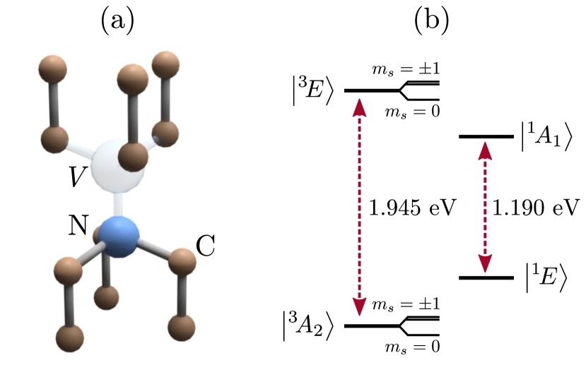
Figure 1: (a) Atomic structure of the nitrogen-vacancy center in diamond. (b) Electronic level diagram of $\rm{NV}^{-}$. Energies of the ZPL between the triplets and the singlets are indicated. Spin sublevels of ${}^{3}\!A_{2}$ and ${}^{3}\!E$ states are not to scale.

Experimental measurements of photoionization cross sections and thresholds for the NV center are not straightforward, in particular regarding the photoionization from the excited state ${}^{3}\!E$. The first difficulty is related to the fact that light can induce both the transition $\rm{NV}^{-}\to\rm{NV}^{0}$ (ionization) and $\rm{NV}^{0}\to\rm{NV}^{-}$ (recombination), often making it hard to disentangle the two processes [8, 9, 10]. Moreover, for the NV center in the excited triplet state photoionization competes with stimulated emission, whereby the NV center returns back to the ground state [11, 22], marring the experimental handle of the photoionization process even further. To the best of our knowledge, neither absolute photoionization cross sections from ${}^{3}\!A_{2}$, ${}^{3}\!E$, and ${}^{1}\!E$ states, nor photoionization thresholds from ${}^{3}\!E$ and ${}^{1}\!E$ states have yet been determined experimentally.

In this paper we address the question of the photoionization thresholds and absolute photoionization cross sections using ab-initio calculations. In the two-photon ionization the intra-defect absorption precedes the ionization step. Therefore, we calculate the cross section for that process as well. We also report calculations for the cross section of the stimulated emission from the ${}^{3}\!E$ state. Our work provides important new knowledge about ionization mechanisms that differs from earlier work [9]. The main focus of our work is photoionization from triplet states ${}^{3}\!A_{2}$ and ${}^{3}\!E$. However, we also discuss photoionization from the ${}^{1}\!E$ state. Ab initio treatment of the ${}^{1}\!E$ state is more complicated [23] and we resort to a semi-quantitative analysis based on available experimental data and calculations for the other two states.

This paper is organized as follows. In Sec. II we discuss the mechanism of photoionization of $\rm{NV}^{-}$ centers in more detail. We give the expressions for photoionization thresholds and cross sections, as well as cross sections for intra-defect absorption and stimulated emission. In Sec. III we discuss the particulars of the electronic structure, introduce computational methods and approximations to calculate photoionization thresholds and cross sections, as well as cross sections for intra-defect absorption and stimulated emission. We present the results of calculations and their analysis in Sec. IV. The consequences of our work to the physics of NV centers are discussed in Sec. V. Finally, Sec. VI concludes our work. The target groups of our paper are (i) broad community working on the physics and applications of color centers and (ii) theorists interested in the development of computational methodologies for point defects in solids. The first group can skip a rather technical Sec. III. In the paper we use $\epsilon$ for photon energies, $E$ for electron energies.

II NV center photoionization mechanisms

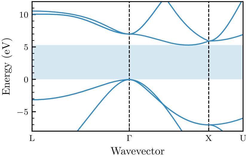
Figure 2: Band structure of bulk diamond calculated using the HSE density functional (see Sec. III for more details about computational methods). The shaded area corresponds to the band gap. Photoionization threshold is determined by electrons being excited to the CBM that occurs between $\Gamma$ and $X$ points.

II.1 Photoionization thresholds

A threshold for photoionization corresponds to electron being excited to the conduction band minimum (CBM). In the case of diamond the CBM occurs along the $\Gamma-X$ line in the Brillouin zone, as shown in Fig. 2.

II.1.1 Photoionization from the ${}^{3}\!A_{2}$ state

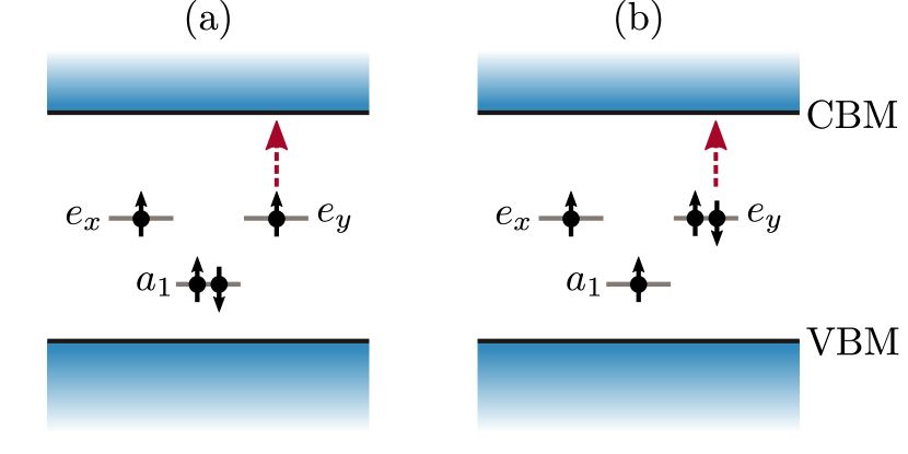
Figure 3: Photoionization of $\rm{NV}^{-}$ center in the single-electron picture. (a) Electronic configuration of the $m_{s}=1$ spin sublevel of the ${}^{3}\!A_{2}$ state. (b) Electronic configuration of the $m_{s}=1$ spin sublevel of the $E_{x}$ component of the ${}^{3}\!E$ manifold. Red arrows show one possibility of photoionization, whereby an $e_{y}$ electron is excited to the conduction band (see text for a more in-depth discussion).

The ground state of $\rm{NV}^{-}$, ${}^{3}\!A_{2}$, is described by an electron configuration $a_{1}^{2}e^{2}$, where $a_{1}$ and $e$ label irreducible representations of single-particle levels [1]. $m_{s}=\pm 1$ spin sublevels of the triplet manifold can be described as single Slater determinants. The $m_{s}=1$ state is illustrated in Fig. 3(a); in the ket notation it can be written as $\mathchoice{\left|a_{1}\bar{a}_{1}e_{x}e_{y}\right\rangle}{|a_{1}\bar{a}_{1}e_{x}e_{y}\rangle}{|a_{1}\bar{a}_{1}e_{x}e_{y}\rangle}{|a_{1}\bar{a}_{1}e_{x}e_{y}\rangle}$, where “bar” indicates spin-down electrons. In the single-particle picture ionization is a process whereby one electron from the $e$ level is excited to the conduction band, turning $\rm{NV}^{-}$ into $\rm{NV}^{0}$. This is illustrated by a red dotted arrow in Fig. 3(a). After the $\rm{NV}^{-}$ is ionized, NV center transitions into the ${}^{2}\!E$ ground state of the neutral center with electron configuration $a_{1}^{2}e^{1}$. The photoionization process can be depicted using the energy-level diagram of the entire system, i.e. $\rm{NV}^{-}$ or $\rm{NV}^{0}$ plus an electron at the CBM, as shown in Fig. 4. Photoionization threshold from the ${}^{3}\!A_{2}$ state, $\mathrm{IP}(^{3}\!A_{2})$, has been measured experimentally by Aslam et al. [10]. Careful study of charge conversion dynamics as a function of wavelength and intensity of laser illumination provided the value $\mathrm{IP}(^{3}\!A_{2})=2.6$ eV; the error bar of this value can be assumed to be ${\sim}0.1$ eV [10]. Previous state-of-the-art theoretical calculations yielded the result $\textrm{IP}(^{3}\!A_{2})=2.64$ eV [24], in excellent agreement with experiment.

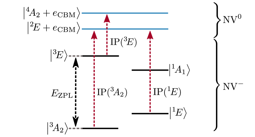
Figure 4: Photoionization of $\rm{NV}^{-}$ from ${}^{3}\!A_{2}$, ${}^{3}\!E$, and ${}^{1}\!E$ states. Horizontal lines indicate the energy of the system: black for $\rm{NV}^{-}$ and blue for $\rm{NV}^{0}$ plus an electron at the CBM. All energies are to scale. Red arrows indicate possible photoionization mechanisms, $E_{\text{ZPL}}$ is the ZPL energy of the triplet transition.

II.1.2 Photoionization from the ${}^{3}\!E$ state

Compared to the photoionization from the ground state, the physics of the photoionization from the ${}^{3}\!E$ state is presently less understood. To the best of our knowledge, the photoionization threshold for photoionization from the excited triplet state is not known. The electronic configuration of the ${}^{3}\!E$ state is $a_{1}^{1}e^{3}$. The $m_{s}=1$ spin sublevel of the $E_{x}$ orbital component, $\mathchoice{\left|a_{1}e_{x}e_{y}\bar{e}_{y}\right\rangle}{|a_{1}e_{x}e_{y}\bar{e}_{y}\rangle}{|a_{1}e_{x}e_{y}\bar{e}_{y}\rangle}{|a_{1}e_{x}e_{y}\bar{e}_{y}\rangle}$, is illustrated in Fig. 3(b). Removing one electron from the $e$ level [red dotted arrow in Fig. 3(b)] yields the configuration $a_{1}^{1}e^{2}$. The lowest-energy state with this configuration is the spin-quartet ${}^{4}\!A_{2}$ state of $\rm{NV}^{0}$. Therefore, the final state of the $\rm{NV}^{0}$ after the photoionization is the meta-stable state ${}^{4}\!A_{2}$ and not the ground state ${}^{2}\!E$, as it was sometimes assumed [9]. The energy-level diagram for this photoionization process is shown in Fig. 4: the initial state is $\rm{NV}^{-}$ in the ${}^{3}\!E$ state, while the final state is $\rm{NV}^{0}$ in the ${}^{4}\!A_{2}$ state plus an electron in the conduction band. The expression for the threshold of photoionization, $\textrm{IP}(^{3}\!E)$, can be read from Fig. 4:

$$\textrm{IP}(^{3}\!E)=\textrm{IP}(^{3}\!A_{2})-E_{\textrm{ZPL}}+\left[E\left({}^{4}\!A_{2}\right)-E\left({}^{2}\!E\right)\right].$$ (1)

The equation above enables the determination of the threshold for the photoionization from the ${}^{3}\!E$ state. Unfortunately, the energy difference $\left[E\left({}^{4}\!A_{2}\right)-E\left({}^{2}\!E\right)\right]$ between the two states of $\rm{NV}^{0}$ is not known experimentally. Therefore, the “experimental” value of $\textrm{IP}(^{3}\!E)$ cannot be deduced from this relationship. Even though the experimental values of $\textrm{IP}(^{3}\!A_{2})$ and $E_{\textrm{ZPL}}$ are known, to benefit from possible cancellation of errors in theoretical calculations, in this paper we will calculate all the quantities that appear in Eq. (1) using the same computational setup, described in Sec. III.

Apart from the ${}^{4}\!A_{2}$ state, there are other $\rm{NV}^{0}$ states with the electron configuration $a_{1}e^{2}$, the lowest of which is ${}^{2}\!A_{2}$ [1]. Using the equation similar to Eq. (1) we can determine the “experimental” threshold for the photoionization via this process to be about 2.8 eV. This is outside the range of energies we consider in this work and therefore this process will be not be analyzed further.

II.1.3 Photoionization from the ${}^{1}\!E$ state

Unlike $m_{s}=\pm 1$ spin sublevels of the triplet states, the two components of the orbital doubled ${}^{1}\!E$ are described by multi-determinant wavefunctions, as discussed in, e.g., Ref. [23]. However, as in the case of ${}^{3}\!A_{2}$, the electronic configuration of the ${}^{1}\!E$ state is $a_{1}^{2}e^{2}$. During the photoionization one $e$ electron is promoted to the conduction band, and NV center transitions to the ${}^{2}\!E$ ground state of the neutral defect with electronic configuration $a_{1}^{2}e^{1}$. It is straightforward to deduce the photoionization threshold from the ${}^{1}\!E$ state (Fig. 4):

$$\textrm{IP}(^{1}\!E)=\textrm{IP}(^{3}\!A_{2})-\left[E\left({}^{1}\!E\right)-E\left({}^{3}\!A_{2}\right)\right].$$ (2)

The energy difference $\left[E\left({}^{1}\!E\right)-E\left({}^{3}\!A_{2}\right)\right]$ has not been measured directly. However, the analysis of the ISC between the ${}^{3}\!E$ and the ${}^{1}\!A_{1}$, as well as the knowledge of the ZPL energy between the two singlets, enables one to determine this energy difference to be about $0.38$ eV [25]. As a result, $\textrm{IP}(^{1}\!E)$ can be estimated to be $2.2\pm 0.1$ eV.

II.2 Photoionization cross sections

The general theory of optical absorption in semiconductors is given in a number of textbooks, e.g., Refs. [26, 27]. Let $\tilde{\sigma}_{\rm{ph}}(\epsilon)$ be the photoionization cross section as a function of photon energy $\epsilon$ in the absence of lattice relaxation. It is given by (cf. Eq. (10.2.4) in Ref. [27]):

$$\tilde{\sigma}_{\rm{ph}}(\epsilon)= \frac{4\pi^{2}\alpha}{3n_{D}}\epsilon\sum_{j}r_{ij}^{2}\delta\left(\epsilon-E_{ij}\right).$$ (3)

Here $\alpha$ is the fine-structure constant and $n_{D}=2.4$ is the refractive index of diamond. Label $i$ denotes the initial state $\Psi_{i}$ and the sum runs over all final states $\Psi_{j}$; $E_{ij}=E_{j}-E_{i}$ is the energy difference between the two states. $\vec{r}_{ij}$ are transition dipole moments (that we will also call optical matrix elements), discussed in Sec. III.2. We consider the absorption light by an ensemble of randomly oriented NV centers. This is the reason for the appearance of the factor $1/3$ in Eq. (3).

Vibrational broadening is introduced by replacing $\delta(\epsilon)$ in Eq. (3) with normalized spectral functions of electron–phonon coupling $A(\epsilon)$ (for a more thorough discussion see, e.g., Refs. [28, 29]). In this case we can write actual cross section as a convolution:

$$\sigma_{\rm{ph}}(\epsilon) =\epsilon\int_{-\infty}^{\infty}\frac{1}{\epsilon^{\prime}}\tilde{\sigma}_{\rm{ph}}(\epsilon^{\prime})A(\epsilon-\epsilon^{\prime})\,\mathrm{d}\epsilon^{\prime}.$$ (4)

Temperature dependence of the photoionization cross section occurs mainly via the temperature dependence of the spectral functions $A(\epsilon)$. In the remainder of the paper we will assume a $T=0$ K limit for these functions.

II.3 Cross section of the intra-defect absorption and stimulated emission

As discussed in Sec. I, photoionization from the ${}^{3}\!E$ state competes with stimulated emission that returns $\rm{NV}^{-}$ back to the ground state ${}^{3}\!A_{2}$. The cross section of stimulated emission (the process ${}^{3}\!E\rightarrow{{}^{3}\!A_{2}}$) is given by an expression:

$$\sigma_{\rm{st}}(\epsilon)=\frac{4\pi^{2}\alpha}{3n_{D}}\epsilon r_{ij}^{2}A\left(E_{\mathrm{ZPL}}-\epsilon\right).$$ (5)

Here $r_{ij}$ is the optical matrix element for the transition ${{}^{3}\!A_{2}}\rightarrow{{}^{3}\!E}$, $E_{\rm{ZPL}}=1.945$ eV, and $A(\epsilon)$ is the spectral function for electron–phonon coupling for stimulated emission, which is identical to that of spontaneous emission (luminescence).

Another important parameter needed to understand the whole two-step photoionization process is the cross section for intra-defect absorption ${}^{3}\!A_{2}\to{{}^{3}\!E}$. Its cross section is given by:

$$\sigma_{\rm{intra}}(\epsilon)=g\frac{4\pi^{2}\alpha}{3n_{D}}\epsilon r_{ij}^{2}A\left(\epsilon-E_{\mathrm{ZPL}}\right).$$ (6)

Here $A(\epsilon)$ is spectral function of electron–phonon coupling for the absorption ${}^{3}\!A_{2}\to{{}^{3}\!E}$, and $g=2$ is the orbital degeneracy factor of the final state ${}^{3}\!E$.

III Theory and methods

III.1 Electronic structure methods

Calculations have been performed within the framework of density functional theory (DFT). For the geometry optimization, as well as the calculation of excitation energies and ionization thresholds we used the hybrid exchange and correlation functional of Heyd, Scuseria, and Ernzerhof (HSE) [30]. In this functional a fraction $a=1/4$ of screened Fock exchange is ad-mixed to the semi-local exchange based on the generalized gradient approximation in the form of Perdew, Burke, and Ernzerhof [31]. As discussed below, in order to obtain converged photoionization cross sections, we have to perform integration on a dense $k$-point grid in the Brillouin zone. Unfortunately, such calculations are computationally too expensive if done with the HSE functional. For this purpose the optical matrix elements have been calculated using the PBE functional. Calculations for selected transitions have shown that HSE and PBE matrix elements differ by less than 10%. We used the projector-augmented wave approach with a plane-wave energy cutoff of 500 eV. Calculations have been performed with the Vienna Ab-initio Simulation Package (Vasp) [32].

HSE functional provides a very good description of diamond, yielding the band gap of $E_{g}=5.34$ eV (experimental value $5.46$ eV), and the lattice constant $a=3.548$ Å (experimental value $3.567$ Å). Geometry relaxation of the NV center has been performed using $4\times 4\times 4$ supercells [33] with 512 atomic sites and a single $\Gamma$ point for the Brillouin zone sampling. Ionization potential from the ground state $\textrm{IP}(^{3}\!A_{2})$ has been determined from computed charge-state transition levels as discussed in, e.g., Ref. [33] with finite-size electrostatic corrections of Ref. [34]. Spectral functions of electron–phonon coupling $A(\epsilon)$ that appear in Eq. (4) have been calculated following the methodology of Ref. [29] (see the Sec. I of the Supplemental Material [35] for a more detailed discussion). Spectral functions for absorption and stimulated emission in Eqs. (5) and (6) have been taken from Ref. [29].

The energies of excited states ${}^{3}\!E$ and ${}^{4}\!A_{2}$ that appear in Eq. (1) have been calculated using the delta-self-consistent-field ($\Delta$SCF) method [36], first applied to the NV center by Gali et al. [37]. To calculate the energy of the ${}^{3}\!E$ state the spin-minority electron in the $a_{1}$ level is promoted to the $e$ level. The total energy of the ${}^{4}\!A_{2}$ state was calculated setting the spin projection to $m_{s}=+3/2$. The $\Delta$SCF method typically performs very well when (i) the state is described by single Slater determinant and (ii) the state has a different spin and/or orbital symmetry from the ground state [36]. This is indeed the case for ${}^{3}\!E$ and ${}^{4}\!A_{2}$ states in with spin projections $m_{s}=\pm 1$ and $m_{s}=\pm 3/2$, respectively.

III.2 The nature of electronic states and calculations of optical matrix elements

The initial state $\Psi_{i}$ that enters in the calculation of the matrix element $\vec{r}_{ij}$ in Eq. (3) represents the entire solid with an embedded negatively charged defect. The final state $\Psi_{j}$ represents the solid with a neutral defect plus an excited electron in the conduction band. The optical matrix element $\vec{r}_{ij}$ and energy difference $E_{ij}$ should then be calculated for these many-electron states. The calculation of the matrix elements for multi-electron wavefunctions is a computationally difficult problem and we will use approximations as described below.

III.2.1 Photoionization from the ${}^{3}\!A_{2}$ state

Let us first assume that $\rm{NV}^{-}$ is initially in the $m_{s}=1$ spin sublevel. As already discussed above, this state can be described by a single Slater determinant $\mathchoice{\left|{}^{3}\!A_{2};1\right\rangle}{|^{3}\!A_{2};1\rangle}{|^{3}\!A_{2};1\rangle}{|^{3}\!A_{2};1\rangle}=\mathchoice{\left|a_{1}\bar{a}_{1}e_{x}e_{y}\right\rangle}{|a_{1}\bar{a}_{1}e_{x}e_{y}\rangle}{|a_{1}\bar{a}_{1}e_{x}e_{y}\rangle}{|a_{1}\bar{a}_{1}e_{x}e_{y}\rangle}$ [Fig. 3(a)]. The final state $\mathchoice{\left|(^{2}\!E_{x/y};\tfrac{1}{2})\nobreak\otimes\nobreak\phi_{c}\right\rangle}{|(^{2}\!E_{x/y};\tfrac{1}{2})\nobreak\otimes\nobreak\phi_{c}\rangle}{|(^{2}\!E_{x/y};\tfrac{1}{2})\nobreak\otimes\nobreak\phi_{c}\rangle}{|(^{2}\!E_{x/y};\tfrac{1}{2})\nobreak\otimes\nobreak\phi_{c}\rangle}=\mathchoice{\left|a_{1}\bar{a}_{1}e_{x/y}\phi_{c}\right\rangle}{|a_{1}\bar{a}_{1}e_{x/y}\phi_{c}\rangle}{|a_{1}\bar{a}_{1}e_{x/y}\phi_{c}\rangle}{|a_{1}\bar{a}_{1}e_{x/y}\phi_{c}\rangle}$ is an antisymmetrized product of $\rm{NV}^{0}$ in the ${}^{2}\!E$ state with spin sublevel $m_{s}=\tfrac{1}{2}$, $\mathchoice{\left|{}^{2}\!E_{x/y};\tfrac{1}{2}\right\rangle}{|^{2}\!E_{x/y};\tfrac{1}{2}\rangle}{|^{2}\!E_{x/y};\tfrac{1}{2}\rangle}{|^{2}\!E_{x/y};\tfrac{1}{2}\rangle}=\mathchoice{\left|a_{1}\bar{a}_{1}e_{x/y}\right\rangle}{|a_{1}\bar{a}_{1}e_{x/y}\rangle}{|a_{1}\bar{a}_{1}e_{x/y}\rangle}{|a_{1}\bar{a}_{1}e_{x/y}\rangle}$, and a spin-up electron in the conduction band with a wavefunction $\phi_{c}$.

Let $\hat{O}=\sum_{i}\vec{r}_{i}$ be the many-electron dipole operator. To simplify the calculation of matrix elements we will assume that all single-electron orbitals from which many-electron wavefunctions are formed are the same in the initial and the final state; the final state differs from initial one by a single occupied orbital, which corresponds to electron in the $e$ state being excited to the conduction band. Such simplification allows to adopt the Slater–Condon rule and reduce the matrix element calculated for a many-body wavefunctions to a matrix element between the two Kohn-Sham states:

$$\vec{r}_{ij}\equiv\mathchoice{\left\langle{}^{3}\!A_{2};1\middle|\hat{O}\middle|(^{2}\!E_{x/y};\tfrac{1}{2})\otimes\phi_{c}\right\rangle}{\langle^{3}\!A_{2};1|\hat{O}|(^{2}\!E_{x/y};\tfrac{1}{2})\otimes\phi_{c}\rangle}{\langle^{3}\!A_{2};1|\hat{O}|(^{2}\!E_{x/y};\tfrac{1}{2})\otimes\phi_{c}\rangle}{\langle^{3}\!A_{2};1|\hat{O}|(^{2}\!E_{x/y};\tfrac{1}{2})\otimes\phi_{c}\rangle}=\mathchoice{\left\langle e_{y/x}\middle|\vec{r}\middle|\phi_{c}\right\rangle}{\langle e_{y/x}|\vec{r}|\phi_{c}\rangle}{\langle e_{y/x}|\vec{r}|\phi_{c}\rangle}{\langle e_{y/x}|\vec{r}|\phi_{c}\rangle}.$$ (7)

As the final state is an orbital doublet, we can calculate, for example, only transition to the $E_{x}$ state and multiply the final result by the degeneracy factor $g=2$. The reasoning for the $m_{s}=-1$ sublevel is analogous, with the only difference that the spin-down electron is excited to the conduction band.

The spin state $m_{s}=0$ is a sum of two Slater determinants $\mathchoice{\left|{}^{3}\!A_{2};0\right\rangle}{|^{3}\!A_{2};0\rangle}{|^{3}\!A_{2};0\rangle}{|^{3}\!A_{2};0\rangle}=1/\sqrt{2}(\mathchoice{\left|a_{1}\bar{a}_{1}{e}_{x}\bar{e}_{y}\right\rangle}{|a_{1}\bar{a}_{1}{e}_{x}\bar{e}_{y}\rangle}{|a_{1}\bar{a}_{1}{e}_{x}\bar{e}_{y}\rangle}{|a_{1}\bar{a}_{1}{e}_{x}\bar{e}_{y}\rangle}+\mathchoice{\left|a_{1}\bar{a}_{1}\bar{e}_{x}{e}_{y}\right\rangle}{|a_{1}\bar{a}_{1}\bar{e}_{x}{e}_{y}\rangle}{|a_{1}\bar{a}_{1}\bar{e}_{x}{e}_{y}\rangle}{|a_{1}\bar{a}_{1}\bar{e}_{x}{e}_{y}\rangle})$. In this case the transition is possible to all four states of the ${}^{2}\!E$ manifold, each with matrix element of the type $\mathchoice{\left\langle e_{y/x}\middle|\vec{r}\middle|\phi_{c}\right\rangle}{\langle e_{y/x}|\vec{r}|\phi_{c}\rangle}{\langle e_{y/x}|\vec{r}|\phi_{c}\rangle}{\langle e_{y/x}|\vec{r}|\phi_{c}\rangle}\sqrt{2}$. The resulting overall cross section is the same as for the $m_{s}=\pm 1$ spin projections.

III.2.2 Photoionization from the ${}^{3}\!E$ state

The situation with the photoionization from the ${}^{3}\!E$ is more delicate. Let us first consider the $m_{s}=1$ spin sublevel with a wavefunction $\mathchoice{\left|{}^{3}\!E_{x/y};1\right\rangle}{|^{3}\!E_{x/y};1\rangle}{|^{3}\!E_{x/y};1\rangle}{|^{3}\!E_{x/y};1\rangle}=\mathchoice{\left|a_{1}e_{x}e_{y}\bar{e}_{y/x}\right\rangle}{|a_{1}e_{x}e_{y}\bar{e}_{y/x}\rangle}{|a_{1}e_{x}e_{y}\bar{e}_{y/x}\rangle}{|a_{1}e_{x}e_{y}\bar{e}_{y/x}\rangle}$. Now there are two different channels for photoionization. (i) A spin-down electron is promoted to the conduction band [red arrow in Fig. 3(b)]. The final state is an antisymmetrized product of $\mathchoice{\left|{}^{4}\!A_{2};\tfrac{3}{2}\right\rangle}{|^{4}\!A_{2};\tfrac{3}{2}\rangle}{|^{4}\!A_{2};\tfrac{3}{2}\rangle}{|^{4}\!A_{2};\tfrac{3}{2}\rangle}$, describing $\rm{NV}^{0}$ in the ${}^{4}\!A_{2}$ manifold with spin projection $m_{s}=3/2$, and a spin-down electron in the conduction band: $\mathchoice{\left|(^{4}\!A_{2};\tfrac{3}{2})\otimes\bar{\phi}_{c}\right\rangle}{|(^{4}\!A_{2};\tfrac{3}{2})\otimes\bar{\phi}_{c}\rangle}{|(^{4}\!A_{2};\tfrac{3}{2})\otimes\bar{\phi}_{c}\rangle}{|(^{4}\!A_{2};\tfrac{3}{2})\otimes\bar{\phi}_{c}\rangle}=\mathchoice{\left|a_{1}e_{x}e_{y}\bar{\phi}_{c}\right\rangle}{|a_{1}e_{x}e_{y}\bar{\phi}_{c}\rangle}{|a_{1}e_{x}e_{y}\bar{\phi}_{c}\rangle}{|a_{1}e_{x}e_{y}\bar{\phi}_{c}\rangle}$. Since both states are single Slater determinants, using the Slater–Condon rule we obtain:

$$\vec{r}_{ij}\equiv\mathchoice{\left\langle{}^{3}\!E_{x/y};1\middle|\hat{O}\middle|(^{4}\!A_{2};\tfrac{3}{2})\otimes\bar{\phi}_{c}\right\rangle}{\langle^{3}\!E_{x/y};1|\hat{O}|(^{4}\!A_{2};\tfrac{3}{2})\otimes\bar{\phi}_{c}\rangle}{\langle^{3}\!E_{x/y};1|\hat{O}|(^{4}\!A_{2};\tfrac{3}{2})\otimes\bar{\phi}_{c}\rangle}{\langle^{3}\!E_{x/y};1|\hat{O}|(^{4}\!A_{2};\tfrac{3}{2})\otimes\bar{\phi}_{c}\rangle}=\mathchoice{\left\langle\bar{e}_{y/x}\middle|\vec{r}\middle|\bar{\phi}_{c}\right\rangle}{\langle\bar{e}_{y/x}|\vec{r}|\bar{\phi}_{c}\rangle}{\langle\bar{e}_{y/x}|\vec{r}|\bar{\phi}_{c}\rangle}{\langle\bar{e}_{y/x}|\vec{r}|\bar{\phi}_{c}\rangle}.$$ (8)

(ii) A spin-up $e$ electron can also be excited to the conduction band. In this case the NV center transitions to the $m_{s}=1/2$ spin sublevel of the ${}^{4}\!A_{2}$ manifold, which is a multi-determinant state. The final state of the entire system can be written as: $\mathchoice{\left|(^{4}\!A_{2};\tfrac{1}{2})\otimes\phi_{c}\right\rangle}{|(^{4}\!A_{2};\tfrac{1}{2})\otimes\phi_{c}\rangle}{|(^{4}\!A_{2};\tfrac{1}{2})\otimes\phi_{c}\rangle}{|(^{4}\!A_{2};\tfrac{1}{2})\otimes\phi_{c}\rangle}=1/\sqrt{3}(\mathchoice{\left|\bar{a}_{1}e_{x}e_{y}\phi_{c}\right\rangle}{|\bar{a}_{1}e_{x}e_{y}\phi_{c}\rangle}{|\bar{a}_{1}e_{x}e_{y}\phi_{c}\rangle}{|\bar{a}_{1}e_{x}e_{y}\phi_{c}\rangle}+\mathchoice{\left|a_{1}\bar{e}_{x}e_{y}\phi_{c}\right\rangle}{|a_{1}\bar{e}_{x}e_{y}\phi_{c}\rangle}{|a_{1}\bar{e}_{x}e_{y}\phi_{c}\rangle}{|a_{1}\bar{e}_{x}e_{y}\phi_{c}\rangle}+\mathchoice{\left|a_{1}e_{x}\bar{e}_{y}\phi_{c}\right\rangle}{|a_{1}e_{x}\bar{e}_{y}\phi_{c}\rangle}{|a_{1}e_{x}\bar{e}_{y}\phi_{c}\rangle}{|a_{1}e_{x}\bar{e}_{y}\phi_{c}\rangle})$. Applying the Slater–Condon rule we obtain:

$$\vec{r}_{ij}\equiv\mathchoice{\left\langle{}^{3}\!E_{x/y};1\middle|\hat{O}\middle|(^{4}\!A_{2};\tfrac{1}{2})\otimes{\phi}_{c}\right\rangle}{\langle^{3}\!E_{x/y};1|\hat{O}|(^{4}\!A_{2};\tfrac{1}{2})\otimes{\phi}_{c}\rangle}{\langle^{3}\!E_{x/y};1|\hat{O}|(^{4}\!A_{2};\tfrac{1}{2})\otimes{\phi}_{c}\rangle}{\langle^{3}\!E_{x/y};1|\hat{O}|(^{4}\!A_{2};\tfrac{1}{2})\otimes{\phi}_{c}\rangle}=\frac{1}{\sqrt{3}}\mathchoice{\left\langle{e}_{y/x}\middle|\vec{r}\middle|{\phi}_{c}\right\rangle}{\langle{e}_{y/x}|\vec{r}|{\phi}_{c}\rangle}{\langle{e}_{y/x}|\vec{r}|{\phi}_{c}\rangle}{\langle{e}_{y/x}|\vec{r}|{\phi}_{c}\rangle}.$$ (9)

As the photoionization rate depends on $r_{ij}^{2}$, we see that the probability of the transition to the $m_{s}=1/2$ sublevel of the ${}^{4}\!A_{2}$ manifold is 3 times smaller than to the $m_{s}=3/2$ sublevel (we will ignore the difference between matrix elements calculated for spin-up and spin-down Kohn-Sham states). Formally, when evaluating the total photoionization cross section pertaining to the $m_{s}=1$ sublevel of the ${}^{3}\!E$ state via Eq. (3), we can consider only the excitation of the spin-down electron and multiply the final result by the “degeneracy factor” $g=4/3$. This is the procedure we have chosen in this work. Analogous reasoning holds for the photoionization from the $m_{s}=-1$ spin sublevel.

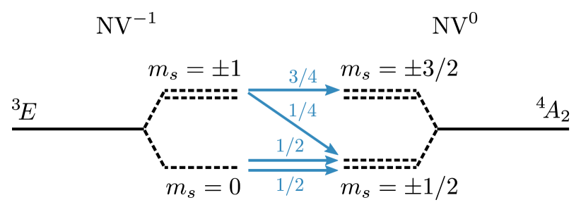
Figure 5: Spin physics of the photoionization from the ${}^{3}\!E$ state. Numbers near arrows show relative probabilities of the transition during photoionization. The $m_{s}=+1$ ($-1$) spin sublevel transitions into either the $m_{s}=+3/2$ ($-3/2$) or the $m_{s}=+1/2$ ($-1/2$) sublevel of the ${}^{4}\!A_{2}$ manifold with different probabilities. The $m_{s}=0$ sublevel transitions to the $m_{s}=\pm 1/2$ sublevels with equal probability. Spin sublevels are separated by zero-field splittings $D(^{3}\!E)=1.42$ GHz [1] and $D(^{4}\!A_{2})=1.69$ GHz [38].

If $\rm{NV}^{-}$ is initially in the $m_{s}=0$ sublevel $\mathchoice{\left|{}^{3}\!E_{x/y};0\right\rangle}{|^{3}\!E_{x/y};0\rangle}{|^{3}\!E_{x/y};0\rangle}{|^{3}\!E_{x/y};0\rangle}=1/\sqrt{2}(\mathchoice{\left|a_{1}\bar{e}_{x}e_{y/x}\bar{e}_{y/x}\right\rangle}{|a_{1}\bar{e}_{x}e_{y/x}\bar{e}_{y/x}\rangle}{|a_{1}\bar{e}_{x}e_{y/x}\bar{e}_{y/x}\rangle}{|a_{1}\bar{e}_{x}e_{y/x}\bar{e}_{y/x}\rangle}+\mathchoice{\left|\bar{a}_{1}e_{x}e_{y/x}\bar{e}_{y/x}\right\rangle}{|\bar{a}_{1}e_{x}e_{y/x}\bar{e}_{y/x}\rangle}{|\bar{a}_{1}e_{x}e_{y/x}\bar{e}_{y/x}\rangle}{|\bar{a}_{1}e_{x}e_{y/x}\bar{e}_{y/x}\rangle})$, the final state of $\rm{NV}^{0}$ is either the $m_{s}=1/2$ or the $m_{s}=-1/2$ sublevel of the ${}^{4}\!A_{2}$ manifold. Following the same reasoning as above one can show that optical matrix elements for these transitions are of the type $\sqrt{2/3}\mathchoice{\left\langle e_{y/x}\middle|\vec{r}\middle|\phi_{c}\right\rangle}{\langle e_{y/x}|\vec{r}|\phi_{c}\rangle}{\langle e_{y/x}|\vec{r}|\phi_{c}\rangle}{\langle e_{y/x}|\vec{r}|\phi_{c}\rangle}$. The resulting cross section is identical to the cross section in the case of $m_{s}=\pm 1$ states. Relative transition probabilities between spin sublevels of ${}^{3}\!E$ and ${}^{4}\!A_{2}$ manifolds are summarized in Fig. 5.

III.2.3 Photoionization from the ${}^{1}\!E$ state

The two orbital components of the ${}^{1}\!E$ state can be written as $\mathchoice{\left|{}^{1}\!E_{x}\right\rangle}{|^{1}\!E_{x}\rangle}{|^{1}\!E_{x}\rangle}{|^{1}\!E_{x}\rangle}=1/\sqrt{2}(\mathchoice{\left|a_{1}\bar{a}_{1}e_{x}\bar{e}_{x}\right\rangle}{|a_{1}\bar{a}_{1}e_{x}\bar{e}_{x}\rangle}{|a_{1}\bar{a}_{1}e_{x}\bar{e}_{x}\rangle}{|a_{1}\bar{a}_{1}e_{x}\bar{e}_{x}\rangle}-\mathchoice{\left|a_{1}\bar{a}_{1}{e}_{y}\bar{e}_{y}\right\rangle}{|a_{1}\bar{a}_{1}{e}_{y}\bar{e}_{y}\rangle}{|a_{1}\bar{a}_{1}{e}_{y}\bar{e}_{y}\rangle}{|a_{1}\bar{a}_{1}{e}_{y}\bar{e}_{y}\rangle})$ and $\mathchoice{\left|{}^{1}\!E_{y}\right\rangle}{|^{1}\!E_{y}\rangle}{|^{1}\!E_{y}\rangle}{|^{1}\!E_{y}\rangle}=1/\sqrt{2}(\mathchoice{\left|a_{1}\bar{a}_{1}\bar{e}_{x}{e}_{y}\right\rangle}{|a_{1}\bar{a}_{1}\bar{e}_{x}{e}_{y}\rangle}{|a_{1}\bar{a}_{1}\bar{e}_{x}{e}_{y}\rangle}{|a_{1}\bar{a}_{1}\bar{e}_{x}{e}_{y}\rangle}-\mathchoice{\left|a_{1}\bar{a}_{1}{e}_{x}\bar{e}_{y}\right\rangle}{|a_{1}\bar{a}_{1}{e}_{x}\bar{e}_{y}\rangle}{|a_{1}\bar{a}_{1}{e}_{x}\bar{e}_{y}\rangle}{|a_{1}\bar{a}_{1}{e}_{x}\bar{e}_{y}\rangle})$ [39]. Following the same reasoning as above, one can show that after ionization the NV center transitions to any of the four states of the ${}^{2}\!E$ manifold of $\rm{NV}^{0}$ with equal probability. The photoionization process is described by matrix elements of the type $1/\sqrt{2}\mathchoice{\left\langle e_{x/y}\middle|\vec{r}\middle|\phi_{c}\right\rangle}{\langle e_{x/y}|\vec{r}|\phi_{c}\rangle}{\langle e_{x/y}|\vec{r}|\phi_{c}\rangle}{\langle e_{x/y}|\vec{r}|\phi_{c}\rangle}$. Due to a multi-determinant nature of ${}^{1}\!E$, the application of a simple $\Delta$SCF procedure to calculate its energy is not straightforward. From the theoretical standpoint, there is no consensus regarding the position of this state above the ${}^{3}\!A_{2}$ ground state [1]. However, as discussed in Sec. II.1.3, energy difference of $\left[E\left({}^{1}\!E\right)-E\left({}^{3}\!A_{2}\right)\right]=0.38$ eV was obtained in Ref. [25]. The main focus of the current paper is photoionization from the triplet states, so in the case of photoionization from ${}^{1}\!E$ our calculations will be more approximate. To make calculations possible we will assume that optical matrix elements are identical to those of the photoionization from the ${}^{3}\!A_{2}$ state. In addition, we will use the same spectral function $A(\epsilon)$ as for the ground state, ignoring the occurrence of the Jahn-Teller effect in the ${}^{1}\!E$ state. The resulting cross section is then nearly identical to of the ${}^{3}\!A_{2}$ state, with the only difference that the energies that appear in Eqs. (3) and (4) differ for the two processes.

III.2.4 Calculation of optical matrix elements and transition energies

The application of the Slater–Condon rule enables us to evaluate the transition dipole moment $\vec{r}_{ij}$ for Kohn-Sham states $\psi_{i}$ and $\psi_{j}$ rather than many-electron states $\Psi_{i}$ and $\Psi_{j}$. As the position operator is not well-defined in periodic boundary conditions, matrix elements are calculated as $\vec{r}_{ij}=\langle u_{i}|i\vec{\nabla}_{\vec{k}}|u_{j}\rangle$, were $u_{i}$ and $u_{j}$ are lattice-periodic parts of wavefunctions $\psi_{i}$ and $\psi_{j}$. Eq. (3) is often alternatively formulated in terms of momentum matrix elements [26], defined as $\vec{p}_{ij}=im(\epsilon/\hbar)\vec{r}_{ij}$.

When replacing the many-electron formulation with the formulation based on Kohn-Sham states, $E_{ij}$ in Eq. (3) is the difference between Kohn–Sham eigenvalues of the defect state and the perturbed bulk state. Since the smallest value of $E_{ij}$ does not necessarily correspond to photoionization thresholds, obtained from total energy calculations [$\textrm{IP}(^{3}\!A_{2})$ or $\textrm{IP}(^{3}\!E)$], we apply a rigid shift so that calculated cross sections are consistent with thresholds. As discussed in Sec. III.2.3, the calculations for the ${}^{1}\!E$ state are more approximate. In this case we use Kohn-Sham states pertaining to the ${}^{3}\!A_{2}$ ground state, but the rigid shift of energies corresponds to the “experimental” threshold $\textrm{IP}(^{1}\!E)$.

III.3 The choice of the charge state

When replacing many-electron wavefunctions with single-particle ones, an important issue arises regarding the charge state for which single-particle energies and single-particle Kohn–Sham states are calculated. On the one hand, since a negatively charged defect is the one that is being ionized, performing calculations for a defect in the $q=-1$ charge state could seem natural. However, while the defect wavefunctions are represented correctly in this charge state, conduction band wavefunctions are not. Indeed, the final state $\psi_{j}$ is a conduction band state perturbed by the neutral defect, and not a negative one. As a result of long-range Coulomb interactions these perturbations are much more significant for the negatively charged defect. On the other hand, supercell calculations of the neutral NV center adequately capture perturbations to the conduction bands, but these calculations do not give a totally accurate account of the initial defect state. The question is then: which of the two calculations approximates the calculation based on many-electron wavefunctions better? Due to a localized nature of defect states we can expect that the difference of their single-particle Kohn–Sham wavefunctions calculated in two charge states, $q=0$ and $q=-1$, is much smaller than the corresponding difference between delocalized perturbed bulk states. Following the methodology of Ref. [40] we estimated overlap integrals between defect levels in the case of the neutral and the negatively charged defect. Our result show that more than 99.6% of the wavefunction character is preserved when the charge state is changed. We conclude that performing calculations in the neutral charge state is a much more accurate approximation. This approximation will be employed in this paper.

III.4 Brillouin zone integration and supercell effects

In the supercell formulation, one obtains an appropriately normalized cross section if one replaces the sum over $j$ in Eq. (3) with the sum over $k$-points of the Brillouin zone of the supercell via $\sum_{j}\rightarrow 1/N\sum_{n,\vec{k}}$, where $N$ is the number of uniformly distributed $k$-points and $n$ runs over all conduction bands states for a fixed $\vec{k}$. Matrix elements $\vec{r}_{ij}$ are calculated between the defect state and the perturbed conduction band state (normalized in the supercell) for the same $\vec{k}$. In practice the sum is performed in the irreducible wedge of the Brillouin zone.

In order to converge the cross section $\sigma_{\rm{ph}}(\epsilon)$ for a given supercell, a very dense $k$-point mesh is required. Increasing the mesh in self-consistent calculations of supercells becomes computationally very expensive even at the PBE level. Charge density converges much faster as the $k$-point mesh is increased. Thus, we performed self-consistent calculations using the $6\times 6\times 6$ Monkhorst-Pack $k$-point mesh for the charge density. Photoionization cross sections have been calculated by performing non-self-consistent calculations using much denser $14\times 14\times 14$ meshes. In this way one obtains photoionization cross sections of a periodically repeated array of NV centers (albeit correctly normalized per one absorber).

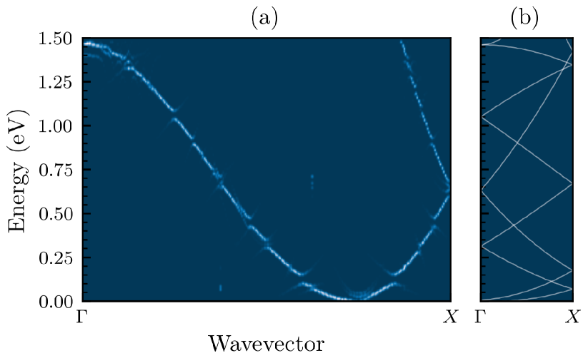
Figure 6: (a) Unfolded band structure of conduction band states perturbed by the NV center along the $\Gamma\mbox{--}X$ path. The color indicates a relative spectral weight (dark blue is zero), see Ref. [41] for more details. (b) The band structure of bulk diamond, folded to the first Brillouin zone of the $4\times 4\times 4$ supercell along the $\Gamma\mbox{--}X$ path of the supercell.

Artificial periodicity of the supercell approach gives rise to two undesirable effects: (i) defect–defect interaction and (ii) spurious perturbation of conduction band states. Aspect (i) affects defect wavefunctions. To check the convergence of these wavefunctions as a function of the supercell size one can, for example, calculate the optical matrix element $\vec{r}_{ij}$ [Eqs. (5) and (6)] for the transition between $a_{1}$ and $e$ levels of the NV center. The comparison of $4\times 4\times 4$ and $5\times 5\times 5$ supercells shows that matrix elements calculated in these two supercells differ by less than 3%.

Effect (ii), however, is more subtle. Periodically repeated NV centers form a superlattice and one could expect the formation of sub-bands and the opening of “mini-gaps” in the same way it occurs in traditional semiconductor superlattices. This is indeed what we observe. In Fig. 6(a) we show the band structure of the $4\times 4\times 4$ supercell unfolded [41] onto the Brillouin zone of a primitive diamond cell. For illustration purposes we choose the band structure of a neutral NV in the ${}^{4}\!A_{2}$ state. In Fig. 6(a) one can clearly identify discontinuities in the band structure. To understand why these discontinuities form at specific energies and $k$ vectors, in Fig. 6(b) we show the band structure of bulk diamond folded onto Brillouin zone of the $4\times 4\times 4$ supercell. Such folding introduces degeneracies at the band crossing points and Brillouin zone boundaries. When perturbations, such as the potential of periodically repeated NV centers, are present, these degeneracies are removed, explaining the formation of “mini-gaps” in Fig. 6(a). Apart from the density of states (DOS), we find that the values optical matrix element $\vec{r}_{ij}$ are also affected by artificial periodicity. We observe jumps of $r^{2}_{ij}$ across the “mini gaps”. These jumps can be explained using the textbook picture of the behavior of electronic wavefunctions close to the band gap in pristine solids via the formation of standing electronic waves (see, e.g., Fig. 3 in Chapter 7 of Ref. [42]). The wave-function on one edge of the “mini-gap” has a vanishing weight on the NV center and $\vec{r}_{ij}$ pertaining to this state tends to zero. The wavefunction on the other edge has maximum weight on the NV center, and $\vec{r}_{ij}$ pertaining to that state attains a finite value. We conclude that artificial periodicity affects both the energies of conduction band states and the values of optical matrix elements. This is the origin for our observed slow convergence of calculated cross sections as a function of the supercell (not shown), even when the Brillouin zone integration itself is already converged.

In this paper we use the following ad hoc solution to this problem. (i) Each perturbed conduction band state of the defect supercell is unfolded to the Brillouin zone of the primitive cell using the methodology of Ref. 41. Each $k$-point of the Brillouin zone of the defect supercell unfolds onto several $k$-points of the Brillouin zone of the primitive cell. (ii) We take the $k$-vector with the highest spectral weight and find the bulk state with the same $k$ which is closest in energy (typical differences $<0.08$ eV). This is the energy that we use in Eq. (3). In this way we get rid of the discontinuities of the conduction band state energies. The procedure also yields the band index $n$. In the case of degeneracy this $k$-point is assigned to multiple $n$’s. (iii) For a given perturbed conduction band state the value of the optical matrix element $r^{2}_{ij}$ is averaged in the Brillouin zone of the primitive cell. The averaging is performed for each $n$ separately, taking the mean of the points situated closer than $\Delta r_{k}=0.57$ nm^-1 in the reciprocal lattice. This “smears” the jumps of the optical matrix elements across “mini gaps”. The overall procedure results in smooth calculated values of $\sigma_{\rm{ph}}(\epsilon)$ as a function of $\epsilon$. The effect of such smoothing is illustrated in Sec. II of the Supplemental Material [35].

III.5 Local-field effects

In the expressions for photoionization cross sections (3), (5), and (6) we have omitted so-called local-field effects [27, 26]. These effects appear due to the scattering of light on the defect, which can result in the electric field on the defect site being different from that in the bulk. Historically, these effects have been included phenomenologically by multiplying the cross sections by an enhancement factor ${(\mathcal{E}_{\rm{eff}}/\mathcal{E}_{0})}^{2}$. Here $\mathcal{E}_{\rm{eff}}$ is the electric field on the defect site, while $\mathcal{E}_{0}$ is the electric field in the bulk. Classical considerations lead to a variety of models [26, 27], from which the so-called Onsager model typically performs best, even though it slightly overestimates the enhancement factor (see Table 10.3 in Ref. [27]). In the Onsager model the ratio between fields is given by:

$$\frac{\mathcal{E}_{\rm{eff}}}{\mathcal{E}_{0}}=\frac{3\varepsilon_{\infty}}{2\varepsilon_{\infty}+1},$$ (10)

where $\varepsilon_{\infty}$ is the dielectric constant of diamond. Using $\varepsilon_{\infty}=5.7$, we obtain $(\mathcal{E}_{\rm{eff}}/\mathcal{E}_{0})=1.38$.

An alternative method to estimate local-field effects is empirical. Radiative emission rate for the ${{}^{3}\!E}\to{{}^{3}\!A_{2}}$ transition is given via:

$$\Gamma_{\rm{rad}}=\frac{1}{\tau_{\rm{rad}}}={\left(\frac{\mathcal{E}_{\rm{eff}}}{\mathcal{E}_{0}}\right)}^{2}\frac{n_{D}E_{\rm{ZPL}}^{3}r_{ij}^{2}}{3\pi\varepsilon_{0}c^{3}\hbar^{4}}.$$ (11)

Here $\varepsilon_{0}$ is vacuum permittivity, and $r_{ij}$ is the transition dipole moment for the transition ${{}^{3}\!E}\to{{}^{3}\!A_{2}}$. Comparing the value calculated without local-field effects with the experimental result can provide an estimate for $(\mathcal{E}_{\rm{eff}}/\mathcal{E}_{0})$. Employing the PBE functional, our calculated radiative lifetime without local field effects is $\tau_{\rm{th}}=12.2$ ns (using the experimental ZPL energy), in excellent accord with the experimental value $\tau=12$ ns [1]. This yields $(\mathcal{E}_{\rm{eff}}/\mathcal{E}_{0})\approx 1.01$. We conclude that the Onsager model over-estimates the value of $(\mathcal{E}_{\rm{eff}}/\mathcal{E}_{0})$, in accord with the results for F-centers in alkali halides [27]. Note, however, that the theoretical value (and therefore possible differences with experiment) are affected not only by the inclusion/exclusion of local fields, but also by other approximations that we employed (density functionals, calculations of matrix elements using Kohn–Sham states, etc.). Regardless, we estimate that in the case of NV centers $(\mathcal{E}_{\rm{eff}}/\mathcal{E}_{0})$ is in the range $(1\mbox{--}1.4)$, and very likely close to $1$. In the remainder of this paper we will therefore set the enhancement factor ${(\mathcal{E}_{\rm{eff}}/\mathcal{E}_{0})}^{2}$ to 1.

IV Results

IV.1 Excitation energies and photoionization thresholds

For the photoionization threshold from the ground state ${}^{3}\!A_{2}$ we obtain the value $\textrm{IP}(^{3}\!A_{2})=2.67$ eV. This is close to the previously published ab-initio result of 2.64 eV [24]. We attribute a small difference of 0.03 eV to a slightly larger kinetic energy cutoff used in the current work, and, probably more importantly, a different finite-size correction scheme (cf. Ref. [34]). Both of the calculated thresholds are in a very good agreement with the experimental one of ${\sim}2.6$ eV, determined in Ref. [10]. This establishes an error bar of about $0.1$ eV for the agreement of ab-initio calculations with experimental data regarding photoionization thresholds.

The ZPL energy of the intra-defect transition ${{}^{3}\!A_{2}}\rightarrow{{}^{3}\!E}$ is found to be $E(^{3}\!E)-E(^{3}\!A_{2})=1.996$ eV. This is again in agreement with previous calculations [37] and the experimental value of $1.945$ eV, exhibiting an accuracy better than $0.1$ eV. Finally, for the energy difference $[E(^{4}\!A_{2})-E(^{2}\!E)]$ in the case of $\rm{NV}^{0}$ we obtain the value of $0.48$ eV. As discussed in Sec. II.1, the experimental energy difference is not available. Previous calculations based on the diagonalization of the Hubbard Hamiltonian (albeit with a rather small basis) [43] yielded a value of 0.68 eV for the vertical transition (i.e., keeping the atoms fixed in the geometry of the ${}^{2}\!E$) state. Including our calculated relaxation energy of 0.12 eV we obtain a corrected value of 0.56 eV, in good agreement with our result. Eventually, using Eq. (1), we obtain the photoionization threshold from the ${}^{3}\!E$ state $\textrm{IP}(^{3}\!E)=1.15$ eV. Calculated and experimental thresholds for photoionization from ${}^{3}\!A_{2}$, ${}^{3}\!E$, and ${}^{1}\!E$ states are summarized in Table 1. Photoionization threshold from the ${}^{1}\!E$ state has not been measured directly, but is deduced from the analysis in Ref. [25].

	$\textrm{IP}(^{3}\!A_{2})$	$\textrm{IP}(^{3}\!E)$	$\textrm{IP}(^{1}\!E)$
theory	2.67	1.15	–
experiment	2.6	–	2.2

Table 1: Thresholds for photoionization from the ${}^{3}\!A_{2}$, ${}^{3}\!E$, and ${}^{1}\!E$ states of $\rm{NV}^{-}$ (in eV). The experimental result for $\textrm{IP}(^{3}\!A_{2})$ from Ref. [10]. The value of $\textrm{IP}(^{1}\!E)$ has not been measured directly, but deduced from Ref. [25] (shown in italic). The assumed experimental error bar of the latter two thresholds is 0.1 eV.

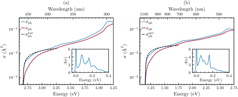
Figure 7: Photoionization cross sections from (a) the ${}^{3}\!A_{2}$ and (b) the ${}^{3}\!E$ state of $\rm{NV}^{-}$. Blue lines: cross sections $\tilde{\sigma}_{\rm{ph}}(\epsilon)$ without vibrational broadening [Eq. (3)]; red lines: actual cross sections $\sigma_{\rm{ph}}(\epsilon)$ [Eq. (4)]; dashed lines show $\tilde{\sigma}_{\rm{ph}}$ calculated using a constant momentum matrix element in Eq. (3) and DOS corresponding to a parabolic band (see text). Insets show the spectral function of electron–phonon coupling $A(\epsilon)$.

IV.2 Cross sections

Before we present the results for NV centers, let us first briefly review some aspects regarding the existing knowledge of photoionization cross sections of deep defects in solids [26]. The overall shape of the function $\tilde{\sigma}_{\rm{ph}}(\epsilon)$ depends on the specifics of the defect wavefunction and of the bulk conduction band structure. Over the years many analytical and semi-analytical models of photoionization of deep defects have been developed [26]. Most of these models use the formulation based on the momentum matrix element $\vec{p}_{ij}=im(\epsilon/\hbar)\vec{r}_{ij}$, which we will also follow in this Section.

For the conduction band with a parabolic dispersion close to the CBM, photoionization threshold corresponds to the excitation to the CBM with the electronic density of states $D(E)\sim{\left(E-E_{\rm{CBM}}\right)}^{1/2}$. In this situation there are two limit cases regarding the dependence of the momentum matrix element $\vec{p}_{ij}$ on $\Delta\vec{k}$, where $\Delta\vec{k}$ is the quasi-momentum measured with respect to the value at the CBM. One limit corresponds to a system where the character of the defect wavefunction is essentially the same as the character of bulk states near the CBM. In this case one obtains [26] $\vec{p}_{ij}\sim\Delta\vec{k}$, which yields the cross section (without electron-phonon coupling) close to the threshold $\tilde{\sigma}_{\rm{ph}}(\epsilon)\sim$${(\epsilon-\epsilon_{\rm{th}})}^{3/2}$. Here $\epsilon_{\rm{th}}$ is the threshold for photoionization, i.e., $\textrm{IP}(^{3}\!A_{2})$, $\textrm{IP}(^{3}\!E)$, or $\textrm{IP}(^{1}\!E)$ from Table 1. One could say that the transition from the defect state to the CBM is dipole-forbidden. Such a scenario is described, e.g., by the widely-used Lucovsky model [44]. Another limit describes a dipole-allowed transition to the CBM. This happens, for example, when the defect state has $p$ character, while the conduction band states have $s$ character, or vice versa. In this case, to a very good approximation, $\vec{p}_{ij}$ is constant for small $\Delta\vec{k}$ [26], and one obtains $\tilde{\sigma}_{\rm{ph}}(\epsilon)\sim$${(\epsilon-\epsilon_{\rm{th}})}^{1/2}$ close to the absorption edge.

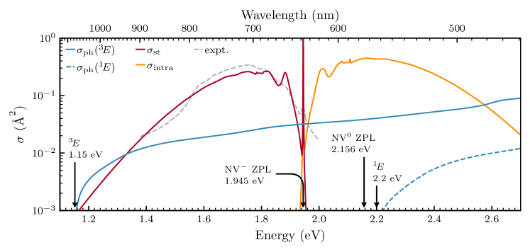
Figure 8: Calculated cross section as a function of photon energy. Solid blue: photoionization from the excited state ${}^{3}\!E$, $\sigma_{\rm{ph}}$; dark red: stimulated emission, $\sigma_{\rm{st}}$; orange: intra-defect absorption, $\sigma_{\rm{intra}}$; dashed blue: photoionization from the singlet state ${}^{1}\!E$. Dashed gray line shows cross section for stimulated emission from Ref. [22]. Photoionization threshold from ${}^{3}\!E$ and ${}^{1}\!E$ are indicated (estimated error bar 0.1 eV), together with the experimental values of the ZPL energy for $\rm{NV}^{-}$ and $\rm{NV}^{0}$.

The photoionization cross section $\tilde{\sigma}_{\rm{ph}}(\epsilon)$ for the ground state ${}^{3}\!A_{2}$ is shown in Fig. 7(a) (blue solid line). $\delta$ functions in Eq. (3) have been replaced by Gaussians with width $\sigma=30$ meV. We find that near the threshold $\tilde{\sigma}_{\rm{ph}}(\epsilon)$$\sim$${(\epsilon-\epsilon_{\rm{th}})}^{1/2}$, indicating that the transition to the band edge is dipole-allowed and the momentum matrix element near the CBM attains a constant value (for more details, see Sec. III of the Supplemental Material [35]). $\tilde{\sigma}_{\rm{ph}}(\epsilon)$ pertaining to this constant value of the momentum matrix element and DOS corresponding to a parabolic band is also shown in Fig. 7(a) (dashed line). The parabolic dispersion is characterized by effective electron masses $m_{\parallel}$ and $m_{\perp}$. In our calculations we used our obtained theoretical values $m_{\parallel}=1.66m_{e}$ and $m_{\perp}=0.32m_{e}$ that are in a good agreement with experimental ones [45]. At larger photon energies $\tilde{\sigma}_{\rm{ph}}(\epsilon)$ starts to deviate from the $\sim$${(\epsilon-\epsilon_{\rm{th}})}^{1/2}$ behavior because the DOS of conduction band states departs from that of the parabolic band and momentum matrix elements start to deviate from a value at the threshold [35]. Lastly and most importantly, Fig. 7(a) shows the actual photoionization cross section $\sigma_{\rm{ph}}(\epsilon)$ (dark red line) that includes the effects of vibrational broadening; the inset depicts the spectral function of electron–phonon coupling $A(\hbar\omega)$ [29, 35]. Vibrational broadening shifts the weight of the cross section to higher energies and $\sigma_{\rm{ph}}(\epsilon)$ no longer exhibits the $\sim$$(\epsilon-\epsilon_{\rm{th}})^{1/2}$ behavior close to the absorption edge. In passing, we note that the results regarding a constant value of $p_{ij}$ around the CBM confirm the assumptions and the value of the momentum matrix element used in our recent calculations on NV centers in diamond nanowires [18].

Calculated cross sections for the photoionization from the ${}^{3}\!E$ state are shown in Fig. 7(b). The behavior of $\tilde{\sigma}_{\rm{ph}}(\epsilon)$ as a function of photon energy $\epsilon$ (blue line) can be explained similarly as for the ground state. In short: (i) close to the threshold $\tilde{\sigma}_{\rm{ph}}(\epsilon)$$\sim$$(\epsilon-\epsilon_{\rm{th}})^{1/2}$ (dashed line); (ii) at larger photon energies $\tilde{\sigma}_{\rm{ph}}(\epsilon)$ starts to deviate from this functional form because the electronic DOS departs from that of the parabolic band and momentum matrix elements can no longer be assumed constant; (iii) actual photoionization cross section $\sigma_{\rm{ph}}(\epsilon)$, which includes the vibrational broadening, exhibits a blue-shift with respect to $\tilde{\sigma}_{\rm{ph}}(\epsilon)$ (dark red line).

The main results of the current paper are presented in Fig. 8. Therein, the photoionization cross section from the excited state ${}^{3}\!E$ (solid blue line) is shown together with the calculated cross sections for stimulation emission $\sigma_{\rm{st}}(\epsilon)$ from the excited state ${}^{3}\!E$ [Eq. (5), dark red line], absorption from the ground state ${{}^{3}\!A_{2}}$ [Eq. (6), orange line], and photoionization cross section from the ${}^{1}\!E$ state (dashed blue line). Photoionization cross section from the ${}^{3}\!A_{2}$ state is not shown. The result for $\sigma_{\rm{st}}(\epsilon)$ is in good agreement with the one presented by Jeske et al. in Ref. [22] (dashed gray line). In that paper the value of the cross section was deduced from the expression identical to Eq. (5), but using the “experimental” value of the optical matrix element and the experimental spectral function $A(\hbar\omega)$. The optical matrix element was calculated from the experimental value of the spontaneous emission rate as in Eq. (11). The consequences of our findings for the physics and technology of NV centers are discussed in the next Section.

V Discussion

V.1 Existing understanding of the photoionization of NV centers

DFT calculations of absorption cross sections from the ground state ${}^{3}\!A_{2}$ have been previously reported in Ref. [46]. Our work differs from the results of these authors in the following aspects: (i) In our work we present absolute values for $\sigma_{\rm{ph}}(\epsilon)$, while in Ref. [46] the cross section has been determined in arbitrary units. (ii) The issues regarding the Brillouin zone integration and supercell size convergence (see Sec. III.4) had not been fully dealt with in Ref. [46], which yielded spurious oscillations of the cross section (Fig. 3 of Ref. [46]). (iii) The coupling to phonons was included in our calculations via the spectral function $A(\hbar\omega)$, while this coupling was omitted from Ref. [46].

The mechanism of the photoionization process from the excited state ${}^{3}\!E$ has been first analyzed in Ref. [9]. These authors suggested that after the photoionization of $\rm{NV}^{-}$ an Auger process takes place, whereby an electron from the conduction band transitions to the $a_{1}$ level, while an electron from the $e$ level is excited to the conduction band. It is our conviction that Auger capture rates have been significantly over-estimated in the calculations of Ref. [9], as they were obtained assuming exceedingly large effective electron densities $\sim$$3\times 10^{20}$ cm^-3. In our opinion, no Auger process takes place. Assuming a realistic electron velocity of $10^{7}$ cm/s after photoionization, one can estimate that within the first picosecond the electron moves away from the NV center by a distance of 100 nm, making any non-radiative capture process very unlikely. Instead, as we propose in the current work, the NV center directly transitions to the ${}^{4}\!A_{2}$ electronic state of $\rm{NV}^{0}$, resulting in the expression for the threshold Eq. (1).

To the best of our knowledge, the details of the photoionization from the ${}^{1}\!E$ states have not been addressed previously.

V.2 ${}^{4}\!A_{2}$ as a state of $\rm{NV}^{0}$ directly after photoionization

The fact that after photoionization from the ${}^{3}\!E$ state NV centers transitions into the metastable ${}^{4}\!A_{2}$ state of $\rm{NV}^{0}$ has important consequences for charge dynamics of NV centers. In particular, this can explain ESR experiments of Ref. [38], where a signal related to the ${}^{4}\!A_{2}$ state was clearly observed. The results of that work allowed the authors to conclude that the existence of a strong ESR signal was due to spin polarization in the ${}^{4}\!A_{2}$ manifold. One possible explanation of spin polarization is that the inter-system crossing from the ${}^{2}\!A_{2}$ excited state of the $\rm{NV}^{0}$ center might lead to spin polarization the same way as it occurs for the negative charge state. However, we propose a different scenario which straightforwardly follows from our results.

The spin physics of the photoionization from the ${}^{3}\!E$ state was discussed in Sec. III.2.2. Fig. 5 summarizes transitions from different sublevels of the ${}^{3}\!E$ manifold of $\rm{NV}^{-}$ to spin sublevels of the ${}^{4}\!A_{2}$ manifold of $\rm{NV}^{0}$. Numbers indicate relative transition probabilities from a given state. In particular, if the defect is initially in the $m_{s}=+1$ ($-1$) spin sublevel, the probability of the transition to the $m_{s}=+3/2$ ($-3/2$) sublevel is $3/4$, while that to the $m_{s}=+1/2$ ($-1/2$) sublevel is $1/4$. If the initial spin state is $m_{s}=0$, after the ionization $\rm{NV}^{0}$ is in any of the $m_{s}=\pm 1/2$ spin states of the ${}^{4}\!A_{2}$ manifold with equal probability. Importantly, one can deduce from Fig. 5 that if $\rm{NV}^{-}$ is initially spin-unpolarized (occupation of different spin sublevels is equal), then there is no spin polarization of the ${}^{4}\!A_{2}$ state after photoionization.

In Ref. [38] the ESR signal pertaining to the ${}^{4}\!A_{2}$ state was only observed for laser wavelengths above the ZPL of the neutral NV center, 2.156 eV [38]. For such illumination the NV center is constantly switching between the negative and the neutral state [8, 10]. When the NV center is in the negative charge state, intrinsic processes within the electronic states of $\rm{NV}^{-}$ lead to a preferential population of the $m_{s}=0$ spin sublevel in the ${}^{3}\!A_{2}$ and the ${}^{3}\!E$ spin triplets [1]. Thus, photoionization mostly occurs from the $m_{s}=0$ sublevel of the ${}^{3}\!E$ state. As per transition probabilities shown in Fig. 5, $m_{s}=\pm 1/2$ spin sublevels of the ${}^{4}\!A_{2}$ are preferentially occupied after the photoionization. $m_{s}=\pm 1/2$ and $m_{s}=\pm 3/2$ spin sublevels are separated by a zero-field splitting $D(^{4}\!A_{2})=1.69$ GHz [38], and thus the population of $m_{s}=\pm 1/2$ sublevels lays ground to a strong ESR signal. In fact, we take the experimental results of Ref. [38] as an indirect confirmation of our proposal regarding the involvement of the ${}^{4}\!A_{2}$ state in the photoionization from the ${}^{3}\!E$ state. Simply put, spin polarization of the ${}^{4}\!A_{2}$ state of $\rm{NV}^{0}$ found in Ref. [38] directly stems from spin polarization of $\rm{NV}^{-}$.

V.3 Spin-to-charge conversion under dual-beam excitation

Turning now to our calculated cross sections and their relevance to the photophysics of NV centers, we emphasize that the body of experimental work on charge-state dynamics at NV centers is large. To consistently interpret all of that work the knowledge of photoionization of $\rm{NV}^{-}$ is often insufficient and the knowledge of similar processes for $\rm{NV}^{0}$ is needed. This is especially true for steady-state experiments, where, depending on the wavelength of laser(s), the NV center can constantly switch between the two charge states. As the study of $\rm{NV}^{0}$ is beyond the scope of the current work, we will focus only on a few selected experiments that we are now able to explain using our data. It is important to stress at the outset that the quality of samples in these studies is crucial. We discuss only experiments done on high-quality bulk samples and will not mention numerous experiments performed on nanodiamonds. The existence of surfaces and possibly various surface defects makes the charge-state dynamics of NV centers in nanodiamonds highly complex and not always reproducible.

One important set of such experiments is spin-to-charge conversion upon dual-beam excitation at cryogenic temperatures [47, 48]. In these protocols one narrow laser is used to resonantly excite $\rm{NV}^{-}$ in a pre-selected spin state, e.g., $m_{s}=0$. Another laser pulse is then used to photoionize the defect from the ${}^{3}\!E$ state. In order not to disturb other spin states, the photoionization is performed with sub-ZPL illumination. In the work of Irber et al. efficient photoionization was obtained using a visible laser emitting at 642 nm (1.93 eV) [48]. At variance, Zhang et al. used a NIR laser emitting at 1064 nm (1.17 eV) [47]; the overall scheme reached high spin read-out fidelities, implying a rather effective photoionization. These results naturally prompt the question: are these two energies, 1.17 eV and 1.93 eV, special?

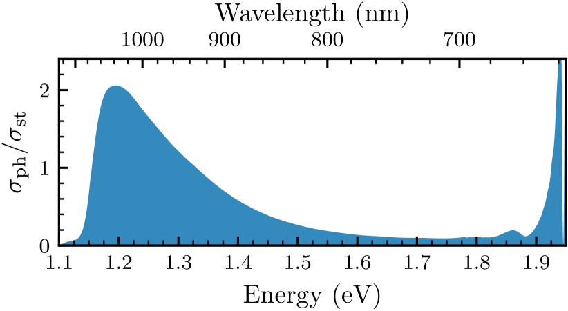
Figure 9: The ratio of the photoionization cross section and the cross section for stimulated emission, $\sigma_{\textrm{ph}}/\sigma_{\textrm{st}}$, as a function of photon energy.

We can now answer this question using the results of our calculations. In Fig. 9 we plot the ratio of the photoionization cross section and that for stimulated emission as a function of photon energy, both from Fig. 8. One can clearly identify two regions where photoionization of $\rm{NV}^{-}$ with sub-ZPL photons is most efficient ($\sigma_{\textrm{ph}}/\sigma_{\textrm{st}}>1$): (i) just above the threshold energy of 1.15 eV, but below $\sim$1.3 eV; (ii) just below the ZPL of 1.945 eV. These are exactly the two energy ranges for which the photoionization was successful in the experiments of Refs. [47, 48]. We note, however, that the exact value of $\sigma_{\textrm{ph}}/\sigma_{\textrm{st}}$ in these two energy windows depends quite sensitively on possible errors in our calculated value of $\textrm{IP}(^{3}\!E)$. Despite this, we conclude that our calculations provide a consistent explanation of the results of Refs. [47] and [48]. Our results point to photon energies where spin-to-charge conversion with sub-ZPL illumination is most efficient. We note that in this work we considered photoionization of an ensemble of randomly oriented NV centers (or, alternatively, photoionization with unpolarized light). In the case of single centers (effectively, excitation and photoionization with polarized light) the ratio $\sigma_{\textrm{ph}}/\sigma_{\textrm{st}}$ depends strongly on polarization. Photoionization of single NVs will be discussed elsewhere.

Finally, we are now in the position to comment on the results of Ref. [11], already mentioned in the Introduction, Sec. I. Studying the luminescence of $\rm{NV}^{0}$ upon illumination with a cw green laser vs. a cw green laser and a pulsed red laser the authors observed that photoionization starts to dominate stimulated emission at below the wavelength of the red laser $\sim$640 nm (1.938 eV). The photoionization threshold from the ${}^{3}\!E$ state was estimated to be $\sim$1.88 eV. The first result is in full agreement with our study. As we show in Fig. 9, photoionization indeed dominates stimulated emission just below the ZPL of 1.945 eV. However, our results show that the threshold for photoionization is 1.15 eV, and not 1.88 eV. The value of 1.88 eV might correspond to the dip in the ratio $\sigma_{\textrm{ph}}/\sigma_{\textrm{st}}$ occurring at about 1.88 eV (Fig. 9). This dip is due increased stimulated emission at this energy (Fig. 8), which in its turn simply reflects the first phonon side-peak in luminescence.

VI Conclusions

In this paper we presented ab-initio calculations of photoionization thresholds and cross sections $\sigma_{\rm{ph}}(\epsilon)$ for the negatively charged nitrogen–vacancy center in diamond. From the point of view of computational materials science, our work presented a new methodology to calculate photoionization cross sections. We employed an integration on a dense $k$-point mesh, together with band unfolding and interpolation, to obtain smooth functions $\sigma_{\rm{ph}}(\epsilon)$ over the entire energy range. To the best of our knowledge, this is the first calculation of absolute photoionization cross sections for point defects using modern electronic structure methods. The methodology is directly applicable to other point defects, including quantum defects [49]. From the point of view of NV physics, we showed that right after the photoionization from the ${}^{3}\!E$ state the $\rm{NV}^{-}$ transitions into the ${}^{4}\!A_{2}$ state of $\rm{NV}^{0}$. This explains spin polarization observed in electron spin resonance experiments of the ${}^{4}\!A_{2}$ state. We determine that the photoionization threshold from the ${}^{3}\!E$ state is 1.15 eV. Together with calculated cross sections, this explains recent experiments on spin-to-charge conversion based on dual-beam excitation [47, 48]. Our work provides important new knowledge about charge-state dynamics of NV centers that was hitherto been missing.

References

- Doherty et al. [2013] M. W. Doherty, N. B. Manson, P. Delaney, F. Jelezko, J. Wrachtrup, and L. C. Hollenberg, The nitrogen-vacancy colour centre in diamond, Phys. Rep. 528, 1 (2013).
- Awschalom et al. [2018] D. D. Awschalom, R. Hanson, J. Wrachtrup, and B. B. Zhou, Quantum technologies with optically interfaced solid-state spins, Nat. Photonics 12, 516 (2018).
- Schirhagl et al. [2014] R. Schirhagl, K. Chang, M. Loretz, and C. L. Degen, Nitrogen-vacancy centers in diamond: Nanoscale sensors for physics and biology, Annu. Rev. Phys. Chem. 65, 83 (2014).
- Hensen et al. [2015] B. Hensen, H. Bernien, A. E. Dréau, A. Reiserer, N. Kalb, M. S. Blok, J. Ruitenberg, R. F. L. Vermeulen, R. N. Schouten, C. Abellán, W. Amaya, V. Pruneri, M. W. Mitchell, M. Markham, D. J. Twitchen, D. Elkouss, S. Wehner, T. H. Taminiau, and R. Hanson, Loophole-free Bell inequality violation using electron spins separated by 1.3 kilometres, Nature 526, 682 (2015).
- Bradley et al. [2019] C. E. Bradley, J. Randall, M. H. Abobeih, R. C. Berrevoets, M. J. Degen, M. A. Bakker, M. Markham, D. J. Twitchen, and T. H. Taminiau, A ten-qubit solid-state spin register with quantum memory up to one minute, Phys. Rev. X 9, 031045 (2019).
- Pezzagna and Meijer [2021] S. Pezzagna and J. Meijer, Quantum computer based on color centers in diamond, Appl. Phys. Rev. 8, 011308 (2021).
- Jelezko et al. [2004] F. Jelezko, T. Gaebel, I. Popa, A. Gruber, and J. Wrachtrup, Observation of coherent oscillations in a single electron spin, Phys. Rev. Lett. 92, 076401 (2004).
- Beha et al. [2012] K. Beha, A. Batalov, N. B. Manson, R. Bratschitsch, and A. Leitenstorfer, Optimum photoluminescence excitation and recharging cycle of single nitrogen-vacancy centers in ultrapure diamond, Phys. Rev. Lett. 109, 097404 (2012).
- Siyushev et al. [2013] P. Siyushev, H. Pinto, M. Vörös, A. Gali, F. Jelezko, and J. Wrachtrup, Optically controlled switching of the charge state of a single nitrogen-vacancy center in diamond at cryogenic temperatures, Phys. Rev. Lett. 110, 167402 (2013).
- Aslam et al. [2013] N. Aslam, G. Waldherr, P. Neumann, F. Jelezko, and J. Wrachtrup, Photo-induced ionization dynamics of the nitrogen vacancy defect in diamond investigated by single-shot charge state detection, New J. Phys. 15, 013064 (2013).
- Jeske et al. [2017] J. Jeske, D. W. M. Lau, X. Vidal, L. P. McGuinness, P. Reineck, B. C. Johnson, M. W. Doherty, J. C. McCallum, S. Onoda, F. Jelezko, T. Ohshima, T. Volz, J. H. Cole, B. C. Gibson, and A. D. Greentree, Stimulated emission from nitrogen-vacancy centres in diamond, Nat. Commun. 8, 14000 (2017).
- Bourgeois et al. [2015] E. Bourgeois, A. Jarmola, P. Siyushev, M. Gulka, J. Hruby, F. Jelezko, D. Budker, and M. Nesladek, Photoelectric detection of electron spin resonance of nitrogen-vacancy centres in diamond, Nat. Commun. 6, 8577 (2015).
- Siyushev et al. [2019] P. Siyushev, M. Nesladek, E. Bourgeois, M. Gulka, J. Hruby, T. Yamamoto, M. Trupke, T. Teraji, J. Isoya, and F. Jelezko, Photoelectrical imaging and coherent spin-state readout of single nitrogen-vacancy centers in diamond, Science 363, 728 (2019).
- Gulka et al. [2021] M. Gulka, D. Wirtitsch, V. Ivády, J. Vodnik, J. Hruby, G. Magchiels, E. Bourgeois, A. Gali, M. Trupke, and M. Nesladek, Room-temperature control and electrical readout of individual nitrogen-vacancy nuclear spins, arXiv:2101.04769 (2021), unpublished.
- Waldherr et al. [2011] G. Waldherr, J. Beck, M. Steiner, P. Neumann, A. Gali, T. Frauenheim, F. Jelezko, and J. Wrachtrup, Dark states of single nitrogen-vacancy centers in diamond unraveled by single shot NMR, Phys. Rev. Lett. 106, 157601 (2011).
- Shields et al. [2015] B. J. Shields, Q. P. Unterreithmeier, N. P. de Leon, H. Park, and M. D. Lukin, Efficient readout of a single spin state in diamond via spin-to-charge conversion, Phys. Rev. Lett. 114, 136402 (2015).
- Hopper et al. [2018] D. A. Hopper, H. J. Shulevitz, and L. C. Bassett, Spin readout techniques of the nitrogen-vacancy center in diamond, Micromachines 9, 437 (2018).
- Oberg et al. [2019] L. M. Oberg, E. Huang, P. M. Reddy, A. Alkauskas, A. D. Greentree, J. H. Cole, N. B. Manson, C. A. Meriles, and M. W. Doherty, Spin coherent quantum transport of electrons between defects in diamond, Nanophotonics 8, 1975 (2019).
- Ulbricht and Loh [2018] R. Ulbricht and Z.-H. Loh, Excited-state lifetime of the infrared transition in diamond, Phys. Rev. B 98, 094309 (2018).
- Acosta et al. [2010] V. M. Acosta, A. Jarmola, E. Bauch, and D. Budker, Optical properties of the nitrogen-vacancy singlet levels in diamond, Phys. Rev. B 82, 201202(R) (2010).
- Hopper et al. [2016] D. A. Hopper, R. R. Grote, A. L. Exarhos, and L. C. Bassett, Near-infrared-assisted charge control and spin readout of the nitrogen-vacancy center in diamond, Phys. Rev. B 94, 241201(R) (2016).
- Nair et al. [2020] S. R. Nair, L. J. Rogers, X. Vidal, R. P. Roberts, H. Abe, T. Ohshima, T. Yatsui, A. D. Greentree, J. Jeske, and T. Volz, Amplification by stimulated emission of nitrogen-vacancy centres in a diamond-loaded fibre cavity, Nanophotonics 9, 4505 (2020).
- Gali et al. [2008] A. Gali, M. Fyta, and E. Kaxiras, Ab initio supercell calculations on nitrogen-vacancy center in diamond: Electronic structure and hyperfine tensors, Phys. Rev. B 77, 155206 (2008).
- Deák et al. [2014] P. Deák, B. Aradi, M. Kaviani, T. Frauenheim, and A. Gali, Formation of NV centers in diamond: A theoretical study based on calculated transitions and migration of nitrogen and vacancy related defects, Phys. Rev. B 89, 075203 (2014).
- Goldman et al. [2015] M. L. Goldman, M. W. Doherty, A. Sipahigil, N. Y. Yao, S. D. Bennett, N. B. Manson, A. Kubanek, and M. D. Lukin, State-selective intersystem crossing in nitrogen-vacancy centers, Phys. Rev. B 91, 165201 (2015).
- Ridley [2013] B. K. Ridley, Quantum processes in semiconductors (Oxford University Press, 2013).
- Stoneham [2001] A. M. Stoneham, Theory of defects in solids (Oxford University Press, 2001).
- Alkauskas et al. [2014] A. Alkauskas, B. B. Buckley, D. D. Awschalom, and C. G. Van de Walle, First-principles theory of the luminescence lineshape for the triplet transition in diamond NV centres, New J. Phys. 16, 073026 (2014).
- Razinkovas et al. [2020] L. Razinkovas, M. W. Doherty, N. B. Manson, C. G. Van de Walle, and A. Alkauskas, Vibrational and vibronic structure of isolated point defects: The nitrogen-vacancy center in diamond, arXiv:2012.04320 (2020), unpublished.
- Heyd et al. [2003] J. Heyd, G. E. Scuseria, and M. Ernzerhof, Hybrid functionals based on a screened coulomb potential, J. Chem. Phys. 118, 8207 (2003).
- Perdew et al. [1996] J. P. Perdew, K. Burke, and M. Ernzerhof, Generalized gradient approximation made simple, Phys. Rev. Lett. 77, 3865 (1996).
- Kresse and Furthmüller [1996] G. Kresse and J. Furthmüller, Efficient iterative schemes for ab initio total-energy calculations using a plane-wave basis set, Phys. Rev. B 54, 11169 (1996).
- Freysoldt et al. [2014] C. Freysoldt, B. Grabowski, T. Hickel, J. Neugebauer, G. Kresse, A. Janotti, and C. G. Van de Walle, First-principles calculations for point defects in solids, Rev. Modern Phys. 86, 253 (2014).
- Freysoldt et al. [2009] C. Freysoldt, J. Neugebauer, and C. G. Van de Walle, Fully ab initio finite-size corrections for charged-defect supercell calculations, Phys. Rev. Lett. 102, 016402 (2009).
- [35] See Supplemental Material at [URL will be inserted by publisher] for: (i) calculation of spectral densities of electron-phonon coupling and spectral functions ; (ii) illustration of our procedure for the Brillouin zone integration; (iii) discussion about the energy-dependence of optical matrix elements.
- Jones and Gunnarsson [1989] R. O. Jones and O. Gunnarsson, The density functional formalism, its applications and prospects, Rev. Modern Phys. 61, 689 (1989).
- Gali et al. [2009] A. Gali, E. Janzén, P. Deák, G. Kresse, and E. Kaxiras, Theory of spin-conserving excitation of the N–V center in diamond, Phys. Rev. Lett. 103, 186404 (2009).
- Felton et al. [2008] S. Felton, A. M. Edmonds, M. E. Newton, P. M. Martineau, D. Fisher, and D. J. Twitchen, Electron paramagnetic resonance studies of the neutral nitrogen vacancy in diamond, Phys. Rev. B 77, 081201(R) (2008).
- Doherty et al. [2011] M. W. Doherty, N. B. Manson, P. Delaney, and L. C. L. Hollenberg, The negatively charged nitrogen-vacancy centre in diamond: the electronic solution, New J. Phys. 13, 025019 (2011).
- Turiansky et al. [2020] M. E. Turiansky, A. Alkauskas, M. Engel, G. Kresse, D. Wickramaratne, J.-X. Shen, C. E. Dreyer, and C. G. Van de Walle, Nonrad: Computing nonradiative capture coefficients from first principles, arXiv:2011.07433 (2020), unpublished.
- Popescu and Zunger [2012] V. Popescu and A. Zunger, Extracting versus effective band structure from supercell calculations on alloys and impurities, Phys. Rev. B 85, 085201 (2012).
- Kittel [2004] C. Kittel, Introduction to Solid State Physics (Wiley, 2004).
- Ranjbar et al. [2011] A. Ranjbar, M. Babamoradi, M. Heidari Saani, M. A. Vesaghi, K. Esfarjani, and Y. Kawazoe, Many-electron states of nitrogen-vacancy centers in diamond and spin density calculations, Phys. Rev. B 84, 165212 (2011).
- Lucovsky [1965] G. Lucovsky, On the photoionization of deep impurity centers in semiconductors, Solid State Commun. 3, 299 (1965).
- Nava et al. [1980] F. Nava, C. Canali, C. Jacoboni, L. Reggiani, and S. Kozlov, Electron effective masses and lattice scattering in natural diamond, Solid State Commun. 33, 475 (1980).
- Bourgeois et al. [2017] E. Bourgeois, E. Londero, K. Buczak, J. Hruby, M. Gulka, Y. Balasubramaniam, G. Wachter, J. Stursa, K. Dobes, F. Aumayr, M. Trupke, A. Gali, and M. Nesladek, Enhanced photoelectric detection of NV magnetic resonances in diamond under dual-beam excitation, Phys. Rev. B 95, 041402(R) (2017).
- Zhang et al. [2021] Y. Zhang, Qiand Guo, W. Ji, M. Wang, F. Yin, Junand Kong, Y. Lin, F. Yin, Chunmingand Shi, Y. Wang, and J. Du, High-fidelity single-shot readout of single electron spin in diamond with spin-to-charge conversion, Nat. Commun. 12, 1529 (2021).
- Irber et al. [2021] D. M. Irber, F. Poggiali, F. Kong, M. Kieschnick, T. Lühmann, D. Kwiatkowski, J. Meijer, J. Du, F. Shi, and F. Reinhard, Robust all-optical single-shot readout of nitrogen-vacancy centers in diamond, Nat. Commun. 12, 532 (2021).
- Bassett et al. [2019] L. Bassett, A. Alkauskas, A. Exarhos, and K.-M. Fu, Quantum defects by design, Nanophotonics 8, 1867 (2019).