General self-similar solutions of diffusion equation and related constructions

Abstract

Transport phenomena plays an important role in science and technology. In the wide variety of applications both advection and diffusion may appear. Regarding diffusion, for long times, different type of decay rates are possible for different non-equilibrium systems. After summarizing the existing solutions of the regular diffusion equation, we present not so well known solution derived from three different trial functions, as a key point we present a family of solutions for the case of infinite horizon. By this we tried to make a step toward understanding the different long time decays for different diffusive systems.

I introduction

The process of spreading is a quite common and relatively often occurring phenomena. If the process is sufficiently slow and exhibits certain features then it is called as a diffusion process. When the particle diffuses into it’s own environment than it is called self-diffusion. This kind of diffusion is characterized often by different parameters in different regions of space.

This fundamental question became an enormous scientific field in the last century a historical review can be found in hist1 ; hist2 . Beyond the most studied regular case there are non-linear (or anomalous) non-linear ; degen ; anom , non-local non-loc or even fractional processes frac-dif . Far from completeness we just mention some of the most relevant monographs. In the following we deal with the regular diffusion equation therefore we mention three basic references crank ; Balescu1997 ; sush . It is obvious that this phenomena has an important number of applications in engineering Bennett2013 ; Bird2015 , in meteorology pasquil ; envir in polymer science poly , in finance fin or even in social networks soc .

Beyond the phenomenological macroscopic description of diffusion there are numerous models exist to study the process. For instance the inhomogeneity in a gas means a non-constant density, and usually also an inhomogeneous pressure. General equations of motion of the one component fluid can be found in Balescu1997 . The case of binary diffusion means a diffusion of given particles among other ones which are different. The binary diffusion has interesting properties and eventually spectacular in case if it is visible. Regarding models of binary diffusion, it is worthwhile to mention the Lorentz gas model. In this model certain results have been obtained related to diffusion by Machta and Zwanzig MaZw , Claus and Gaspard ClGa2001 . Connections with non-equilibrium thermodynamics were analyzed in GaNiDo2002 , and MaTeVo2004 . Beyond diffusion Mátyás and Gaspard MaGa2005 discussed diffusion with a simple reaction - isomerization - where not only the diffusion coefficient, but the reaction rate is also evaluated. One may also find diffusive processes where the diffusion is determined by the surroundings or the boundaries or the shape of the surface MaKl2004 ; KlBaMa2004 ; MaBa2011 ; HaHa2018 .

Regarding biological applications, the diffusion equation has an important role at mesoscopic - cell size – scale AnKo2015 , and also in the design of bioreactors Panda .

Diffusive aspects one may find in certain hydrodynamic equations with dissipation If2002 ; Hu2010 ; Ji2009 ; Fa2010 ; Ba2011 ; YeYu2011 ; BaMa2014 or in quantum related systems Wu2010 ; Dai2010 ; Gao2009 .

We find it important to emphasize that the free-particle Schrödinger equation – from mathematical viewpoint – is also a kind of diffusion equation schro1 ; schro2 therefore all the forthcoming analysis could lead to reasonable results for that equation as well.

It is obvious, but we have to state that mathematically heat conduction is similar to diffusion. The field has its mighty literature as well from which we mention two recent monographs heat1 ; heat2 . Regarding numerical methods is worthwhile to mention the solutions obtained in Ko2020a ; Ko2020b .

Similar equations which may take into account certain other perturbations in the system are the telegraph equation which is ”obviously hyperbolic” jos or other telegraph-type equations like the Euler-Poisson-Darboux which can be derived from the modified Fick’s (or Fourier’s) law barna1 ; garra . Another answer is the investigation of the nonlinear hyperbolic system of diffusion flux relaxation and energy conservation equations instead of the second order diffusion equation imre-robi1 ; imre-robi2 . Such first order system may have shock-wave characters as well. The literature of this question is again numerous and we do not go into further details.

As final point we should mention scientific research fields and mathematical problems which grew out of the original diffusion problem such as reaction-diffusion reacdif1 ; reacdif2 , porous media studies porous , surface growth phenomena kpz , fractional diffusion fractional or p-Laplacian plaplace1 ; plaplace2 equations.

II Theory and Results

Having in mind that the general diffusion process is three dimensional we consider only one Cartesian coordinate, therefore the equation reads

$$\frac{\partial C(x,t)}{\partial t}=D\frac{\partial^{2}C(x,t)}{\partial x^{2}},$$ (1)

where $C(x,t)$ is the distributions of the particle concentration in space and time and $D$ is the diffusion coefficient. $C(x,t)$ in the equation above is considered up to a constant, consequently it may also refer to the concentration above or around the average. The function $C(x,t)$ fulfills the necessary smoothness conditions with existing continuous first and second derivatives in respect to time and and space and from physical reasons $D>0$. Numerous physics textbooks gives us the derivation how the fundamental (the Gaussian) solutions can be obtained e.g. crank ; carl ; math ; tham . First, to dispel misunderstandings we have to express one thing clearly, the regular diffusion equation has existence and unicity theorem for initial and boundary problems, but this is not contradictory to our forthcoming analysis. We will apply three different trial functions (or Ansätze [this is the plural form] ) but neither the initial nor the boundary problems are being well defined. The obtained results may fulfill well-defined initial and boundary problems via fixing their integration constants $c_{1}$ and $c_{2}$.

In 1969 Bluman and Cole bluman gave an analysis based on a general symmetry analysis method giving numerous analytic solutions, some of them are expressible with Gaussian or error functions. At this generality, presented below, there was a need of almost all confluent hypergeometric functions, to describe the phenomena. In the following first we give some additional exact solutions of the diffusion equation ending up with an in-depth analysis of the classical self-similar solutions which can have physical applications.

As note zero we must say that with trivial derivation all reader can verify that the functions

$$\left\{t+\frac{Dx^{2}}{2},\hskip 8.53581ptexp(t\mp\sqrt{D}x),\hskip 8.53581ptexp(-t)\cdot(cos[\sqrt{D}x]+sin[\sqrt{D}x])\right\},$$ (2)

are all solutions of Eq (1). These are called separable solutions, the first one is an additive separable solution $C(x,t)=f(t)+g(x)$ and the following two are multiplicative separable $C(x,t)=h(x)\cdot(t)$ solutions in respect to the spatial and temporal variables.) These solutions are usually mentioned in textbook analysis, and will be relevant later on, as we will see. It is also interesting to note, that the traveling wave Ansatz – which mimics the wave properties of the investigated PDE – $C(x,t)=f(x\mp ct)$ automatically gives the exponential solutions.

Beyond the analysis of Bluman and Cole there is an other celebrated work of Clarkson and Kruskal krusk describing the non-classical method of group invariant solutions, which is often used to obtain similarity solutions of (mostly non-linear) PDEs. Originally it was introduced and applied for the Boussinesq equation. Now we apply it to the diffusion equation. (Due to our best knowledge it was not done and not presented in a clear-cut way till now.) The Ansatz has the form of

$$C(x,t)=\beta(x,t)\cdot W(z[x,t])$$ (3)

where all real functions $\alpha,\beta,W$ and $z$ should have existing first continuous derivatives in respect to time and the second existing continuous derivatives in respect to the coordinate $x$, finally $W(z[x,t])$ is a compound function. The method to derive the solution is the following, the first temporal and second spatial derivatives have to be evaluated and replaced into Eq (1) giving

$$\beta_{t}W+\beta W^{\prime}z_{t}=D(\beta_{xx}W+2\beta W^{\prime}z_{x}+\beta_{x}W^{\prime}z_{x}+\beta W^{\prime\prime}(z_{x})^{2}+\beta W^{\prime}z_{xx}),$$ (4)

where the subscripts x and t mean partial derivation in respect to time and coordinate, and prime means derivation of $W(z)$ in respect to $z$. The key idea is the following we should like to have an ordinary differential equation (ODE) for $W$ as independent variable $z$ With reorganization of the terms it reads

$$W^{\prime\prime}(D\beta(z_{x})^{2})+W^{\prime}(\beta z_{t}-2D\beta z_{x}-D\beta_{x}z_{x}-D\beta z_{xx})+W(\beta_{t}-D\beta_{xx})=0.$$ (5)

To solve this expression as an ODE for $W(z)$ we have to fix that the factors of the second, first and zeroth derivative are real constants

$$D\beta(z_{x})^{2}=\tilde{C}_{1},$$ (6)

$$\beta z_{t}-2D\beta z_{x}-D\beta_{x}z_{x}-D\beta z_{xx}=\tilde{C}_{2},$$ (7)

$$\beta_{t}-D\beta_{xx}=\tilde{C}_{3},\hskip 8.53581ptW\neq 0.$$ (8)

There are numerous ways to solve this system. Note, that (8) is identical to the original diffusion equation if $\tilde{C}_{3}=0$. Therefore if we know and kind of solution, (as starting point we may take the trivial solutions of Eq. (2) – which are additive or multiplicative solutions –) then simply integrating Eqs. (6 - 7) and finally the ODE Eq. (5) numerous solutions can be derived. (Finally, it is important to note, that in the original paper of Clarkson and Kruskal there is an additional functions in the Ansatz $C(x,t)=\alpha(x,t)+\beta(x,t)\cdot W(z[x,t])$ which is $\alpha(x,t)$ and is important for non-linear PDE. However for the linear diffusion equation the superposition is valid and we can neglect it.) These mathematically correct solutions become very compound and complicated if we start with the Gaussian solution and has little physical interest.

Before we get to our essential point we show a second kind of solution which – in theory – interpolates the traveling wave Ansatz $C(x,t)=g(x\mp c\cdot t)$ and the disperse self-similar Ansatz of $C(x,t)=t^{-\alpha}f(x/t^{\beta})$. This trial function is called traveling-profile function and was introduced by Benhamidouche behn with the form of

$$C(x,t)=a(t)\cdot h\left(\frac{x-b(t)}{c(t)}\right)=a(t)\cdot h(\omega),$$ (9)

where all $a,b,c$ and $h$ are continuous real functions with existing continuous first temporal and second spatial derivatives and $\omega$ is the new reduced independent variable. The solution method is similar as explained above. Performing the spatial and temporal derivations and substitution back to (1) we arrive to

$$\frac{c^{2}a_{t}}{a}h+ah^{\prime}[b_{t}c-\eta cc_{t}]=Dh^{\prime\prime},\hskip 28.45274pta(t)/c(t)^{2}\neq 0,$$ (10)

where prime means derivation in respect to $\omega$ and subscript t in respect to time. This equation should be an ODE for $h(\omega)$ therefore the coefficients of $h$ and $h^{\prime}$ should be independent of time, should be constants, therefore the following constraints have to be fulfilled:

$$\frac{c^{2}a_{t}}{a}=\tilde{C}_{1},\hskip 28.45274ptb_{t}c=\tilde{C}_{2},\hskip 28.45274ptc_{t}c=\tilde{C}_{3}.$$ (11)

All three solutions can be easily obtained by direct integration, (starting with the last equation) and read

$$c(t)=\mp\sqrt{2\tilde{C}_{3}t+c_{1}},\hskip 5.69054ptb(t)=\frac{\mp\sqrt{2\tilde{C}_{3}t+c_{1}}}{\tilde{C}_{3}}+c_{2},\hskip 5.69054pta(t)=c_{3}(2\tilde{C}_{3}t+c_{1})^{\frac{\tilde{C}_{1}}{2\tilde{C}_{3}}},$$ (12)

finally the solution of the traveling profile shape function is

$$h(\omega)=c_{4}M\left(-\frac{\tilde{C}_{1}}{2\tilde{C}_{3}},\frac{1}{2},\frac{[\tilde{C}_{2}-\tilde{C}_{2}\omega]^{2}}{D\tilde{C}_{3}}\right)+c_{5}U\left(-\frac{\tilde{C}_{1}}{2\tilde{C}_{3}},\frac{1}{2},\frac{[\tilde{C}_{2}-\tilde{C}_{2}\omega]^{2}}{D\tilde{C}_{3}}\right),$$ (13)

where M and U are the Kummer functions NIST with the argument of

$$\omega=\frac{x-b(t)}{c(t)}=\frac{x}{\sqrt{2\tilde{C}_{3}t+c_{1}}}-\frac{c_{2}}{\sqrt{2\tilde{C}_{3}t+c_{1}}}-\frac{}{}\frac{\tilde{C}_{2}}{\tilde{C}_{3}}.$$ (14)

Finally, we concentrate on our main Ansatz, on the self-similar one

$$C(x,t)=t^{-\alpha}f\left(\frac{x}{t^{\beta}}\right)=t^{-\alpha}f(\eta)\hskip 8.53581pt$$ (15)

where $\alpha$ and $\beta$ are the self-similar exponents being real numbers describing the decay and the spreading of the solution is time and space. These properties makes this Ansatz physically extraordinary relevant and was first introduced by Sedov sedov later used by Zel’dowich and Raizer zeld and Barenblatt barenb . In the last decade we applied this trial function to numerous non-linear PDE systems, most of them are from fluid dynamics imre1 but investigated electromagnetic imre2 or quantum mechanical problems imre3 as well. The self-similar analysis have been successfully applied to different systems, where diffusion may also appear NaSi19 ; Sa20 ; KaSuZh20 .

The forthcoming analysis is quite simple, and similar to the former ones. Let’s calculate the first time and second spatial derivative of the Ansatz (15) using the derivation rule of the indirect function and put in into the diffusion equation (1), we arrive at

$$-\alpha t^{-\alpha-1}f(\eta)-\beta t^{-\alpha-1}\eta\frac{df(\eta)}{d\eta}=Dt^{-\alpha-2\beta}\frac{d^{2}f(\eta)}{d\eta^{2}}.$$ (16)

Now comes the crucial point of the reduction mechanism (or the applicability of the Ansatz) if all three terms has the same time dependence, (all exponents are the same) then all can be canceled by an algebraic simplification and a clear-cut ODE is derived for the shape function. So the relation among the all time dependent factors (now only two)

$$t^{-\alpha-1}\hskip 14.22636pt\stackrel{{\scriptstyle?}}{{=}}\hskip 14.22636ptt^{-\alpha-2\beta},$$ (17)

have to investigated. At this point we have to mention that this analysis can be generalized for PDE systems with 4-5 variables even for multiple spatial dimensions as well, e.g. imre1 ; imre2 ; imre3 ; imre4 which makes the method very striking and effective. Compared to the general Lie symmetry analysis the method remains transparent even for a PDE system of 4-5 variables. The analysis of the relations among the self-similar exponents (now for $\alpha,\beta$) can end up with three different scenarios:

• The linear algebraic equation system among the exponents can be overdetermined, which automatically means contradiction. Therefore the system has inherently no physically self-similar power-law decaying or exploding solutions. Such systems are rare but some damped wave equations e.g. telegraph equations are so.

• All exponents have well-defined numerical values, the analysis of the solutions is straightforward, the remaining coupled non-linear ODE system can be analyzed, in some lucky cases even it can be decoupled and in best cases all variables can be expressed with analytic formulas. Such a system is the incompressible Navier-Stokes equation Ba2011 where all exponents have the same numerical value of 1/2, except the time decay of the pressure function which is +1.

• The linear algebraic equation system for the exponents are under-determined, leaving usually one self-similar exponent completely free, which means an extra free parameter in the obtained ODE system, causing a very rich mathematical structure. The free exponent can have either positive or negative sign. Negative values usually result in power-law divergent or exploding solutions in contrary, positive exponents mean power-law decaying solutions which are desirable for dissipative systems. This is the case for the present regular diffusion equation.

For the present diffusion equation, assuming that in (17) the equality strictly holds, after some trivial algebra we get:

$$\alpha=\textrm{arbitrary real number},\hskip 8.53581pt\beta=1/2,$$ (18)

there is a clear-cut time-independent ODE of

$$-\alpha f-\frac{1}{2}\eta f^{\prime}=Df^{\prime\prime}.$$ (19)

With $\alpha=1/2$ the left-hand side of ODE is total derivative and can be integrated getting

$$-\frac{1}{2}\eta f+c_{1}=Df^{\prime},$$ (20)

if the integration constant – which can be interpreted as a source term– is taken to be zero $c_{1}=0$ we get back the usual Gaussian solutions of

$$f(\eta)=c_{2}e^{-\frac{\eta^{2}}{4D}},$$ (21)

from the final solution of

$$C(x,t)=c_{2}t^{-1/2}e^{-\frac{x^{2}}{4Dt}},$$ (22)

we can read, that $\beta$ is responsible for the spreading and $\alpha$ is for the decay of the solution. This is a general, (and very powerful) feature of the self-similar Ansatz that positive $\alpha$ and $\beta$ values always represent decaying and spreading solutions, which have great physical relevance. (This fundamental solution is sometimes referred to as ${\it{source\>type}}$ solution – by mathematicians – because for $t\rightarrow 0$ then $C(x,0)\rightarrow\delta(x)$.)

We will see later on that, $\alpha<0$ values mean exploding solutions which have only mathematical interest in most cases. It is also clear from (22) that no real solutions can be defined for $t<0$.The spreading and decaying properties are visualized on Fig. 1 below.

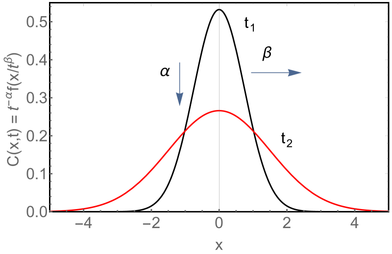
Figure 1: A self-similar solution of Eq. (1) for $t_{1}<t_{2}$. The presented curves are the Gaussians. The physical role of the self-similar exponents are indicated with arrows.

If the more general $c_{1}\neq 0$ is taken then the solutions is changed to

$$f(\eta)=\left(\frac{c_{1}\sqrt{\pi}\cdot erf\left[\frac{1}{2}\sqrt{-\frac{1}{D}}\eta\right]}{D\sqrt{-\frac{1}{D}}}+c_{2}\right)\cdot e^{-\frac{\eta^{2}}{4D}},$$ (23)

where erf is the error function NIST . (We present the formal solutions obtained by the Maple 12 Software [Copyright (c) Maplesoft, a division of Waterloo Inc. 1981 -2008] from now on.) This solutions is not so commonly known. Non zero $c_{1}$ integration constant modifies the shape of the Gaussian solution. For clarity, figure (2) shows the solutions for different initial conditions.

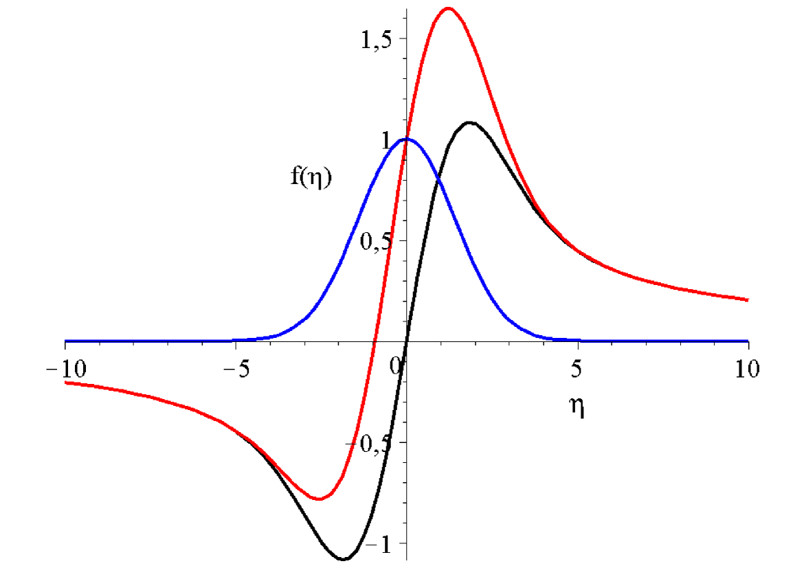
Figure 2: Numerous shape functions $f(\eta)$ Eq. (23) for three different initial conditions the black,red and blue curves are for $c_{1}=1,c_{2}=0$, $c_{1}=c_{2}=1$ and for $c_{1}=0,c_{2}=1$, respectively.

The second – and more general – case is for $\alpha\neq 1/2$, ($\beta$ is still one half) now the solution of Eq. (19) reads:

$$f(\eta)=\eta\cdot e^{-\frac{\eta^{2}}{4D}}\left(c_{1}M\left[1-\alpha,\frac{3}{2},\frac{\eta^{2}}{4D}\right]+c_{2}U\left[1-\alpha,\frac{3}{2},\frac{\eta^{2}}{4D}\right]\right),$$ (24)

where $M(\cdot,\cdot,\cdot)$ and $U(\cdot,\cdot,\cdot)$ are the Kummer’s functions for exhaustive details see the NIST Handbook NIST .

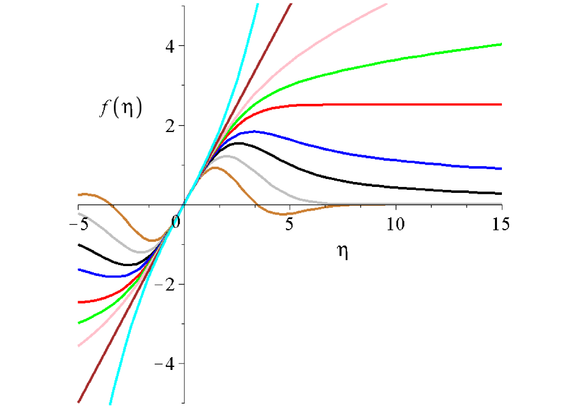
Figure 3: Numerous shape functions $f(\eta)$ Eq. (24) for various $\alpha$s all are for $\beta=1/2$ and for $c_{1}=1,c_{2}=0,D=2$. The gold, gray, black, blue, red, green, pink, brown and cyan curves are for $\alpha=2,1,1/2,1/4,0,-1/8,-1/4,-1/2$ and for $-1$, respectively.

For $\alpha>0$ the solution tends to zero for large values of $\eta$.

For $\alpha<0$ one can see divergent solutions, which go to infinity at infinite argument. (The blow-up type of solutions are different and will be defined later.) From the series expansion of M we get

$$M(a,b,z)=1+\frac{az}{b}+\frac{(a)_{2}z^{2}}{(b)_{2}2!}+...+\frac{(a)_{n}z^{n}}{(b)_{n}n!},$$ (25)

with the $(a)_{n}=a(a+1)(a+2)...(a+n-1),(a)_{0}=1$ is the so-called rising factorial or Pochhammer’s Symbol NIST . In our present case $b$ has a fix non-negative integer value, so none of the solutions have poles at $b=-n$. For the Kummer function $M$ when the parameter $a$ has negative integer numerical values ($a=-m$) the solution is reduced to a polynomial of degree $m$ for the variable $z$. In other cases $a\neq-m$ we get a convergent infinite series for all values of $a,b$ and $z$. There is a connecting formula between the two Kummer functions, $U$ is defined from $M$ via

$$U(a,b,z)=\frac{\pi}{sin(\pi b)}\left(\frac{M[a,b,z]}{\Gamma[1+a-b]\Gamma[b]}-z^{1-b}\frac{M[1+a-b,2-b,z]}{\Gamma[a]\Gamma[2-b]}\right),$$ (26)

where $\Gamma(a)$ is the Gamma function NIST . Figure 3 shows the shape functions for numerous different values of $\alpha$. Note, that all positive $\alpha$s mean solution with asymptotic decay which means that for $\eta\rightarrow\infty$ the $f(\eta)\rightarrow 0$. This can interpreted as certain kind of boundary conditions $f(0)=0$ and $f(\eta\rightarrow\infty)\rightarrow 0$. The $\alpha>0$ means additional oscillations. Zero alpha value means a solution which converges to a finite value, and negative values means divergent solutions.

Note, the clear difference between the two solutions obtained from the traveling profile (13) and the self-similar Ansatz (24). Both contain Kummer functions but with different arguments and coefficient functions.

As one can see, $\alpha=0$ is a special case, when Eq. (19) is simplified to

$$-\frac{\eta f^{\prime}}{2}=Df^{\prime\prime},$$ (27)

resulting

$$f(\eta)=c_{1}+c_{2}\cdot erf\left(\sqrt{\frac{\beta}{2D}}\eta\right),$$ (28)

which is a sigmoid function which starts from zero and tends to a nonzero constant at large values argument $\eta$. As a consequence $C(x,t)$ also tends to a constant for these values.

From practical point of view, this case has certain similarities with the evaporation phenomena evap , when initially there is no vapor concentration above the liquid, and as the time passes above the liquid phase vapor appears, which becomes denser with time.

If $\alpha=1$ we have an interesting case. The first argument of the Kummer functions $M$ and $U$ is $1-\alpha=0$. This means, that

$$M\left(0,\frac{3}{2},\frac{\eta^{2}}{4D}\right)=1,$$ (29)

and the other function $U(0,3/2,\eta^{2}/[4D])$ is also constant. Consequently the general solution is

$$C(x,t)=\frac{1}{t}f(\eta)=\frac{1}{t}\eta e^{-\frac{\eta^{2}}{4D}}\cdot Const.$$ (30)

Case $\alpha=2$ yields more in the expression of the function $f(\eta)$. The first argument of the functions $M$ and $U$ is $1-\alpha=-1$. In this case the function $M$ is a first order polynomial, the higher order coefficients vanishes,

$$M\left(-1,\frac{3}{2},\frac{\eta^{2}}{4D}\right)=1-\frac{2}{3}\frac{\eta^{2}}{4D},$$ (31)

and the function $U$ is also a polynomial with the first order. We can conclude, that the sum of $c_{1}M+c_{2}U$ is also a polynomial with the first order. The general solution reads in this case

$$C(x,t)=\frac{1}{t^{2}}f(\eta)=\frac{1}{t^{2}}\eta e^{-\frac{\eta^{2}}{4D}}\cdot\left(\kappa_{0}+\kappa_{1}\frac{\eta^{2}}{4D}\right),$$ (32)

where $\kappa_{0}$ and $\kappa_{1}$ are real constants.

Following the above argumentation, for $\alpha=n$, (where $n>2$) yields the solution of

$$C(x,t)=\frac{1}{t^{n}}f(\eta)=\frac{1}{t^{n}}\eta e^{-\frac{\eta^{2}}{4D}}\cdot\left(\kappa_{0}+\kappa_{1}\frac{\eta^{2}}{4D}+...+\kappa_{n-1}\cdot\left[\frac{\eta^{2}}{4D}\right]^{n-1}\right).$$ (33)

At this point we try to determine the concrete values of the coefficients $\kappa_{n}$. For the very first case, if $\alpha=1$, there is a single multiplicative constant multiplying the function $f(\eta)$.

For $\alpha=2$, the situation is a little bit more complex. By reinserting the function $f(\eta)$ of formula (32), into the equation (19) we get

$$f(\eta)=\eta\cdot e^{-\frac{\eta^{2}}{4D}}\cdot\kappa_{0}\left[1-\frac{1}{6D}\eta^{2}\right].$$ (34)

If we incorporate the diffusion coefficient by rescaling the time, or if it is taken to be one $D=1$, we have for $C(x,t)$

$$C(x,t)=\frac{1}{t^{2}}f(\eta)=\frac{1}{t^{2}}\eta e^{-\frac{\eta^{2}}{4D}}\cdot\kappa_{0}\left[1-\frac{1}{6}\eta^{2}\right].$$ (35)

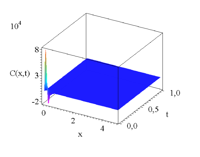
$\alpha=+2$                                                              $\alpha=+1$

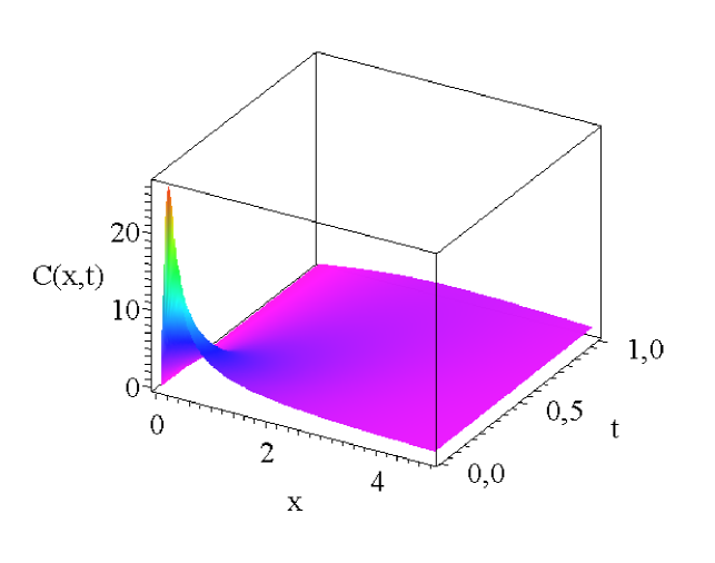
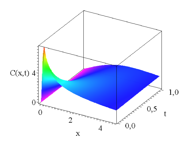
$\alpha=+\frac{1}{2}$                                                              $\alpha=+\frac{1}{4}$

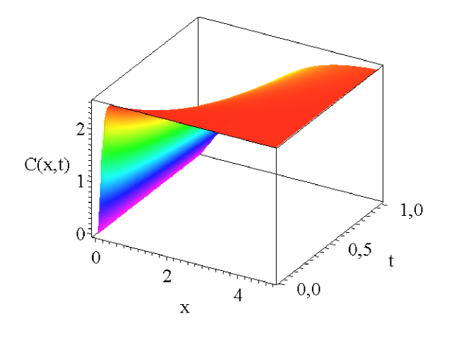
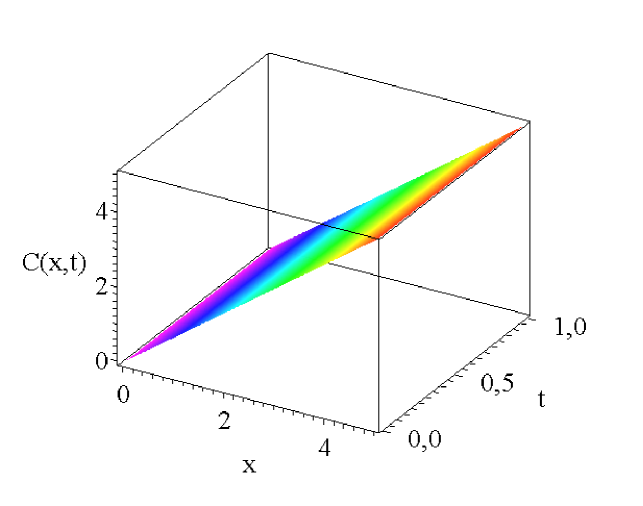
$\alpha=0$                                                              $\alpha=-\frac{1}{2}$

Figure 4: The total solutions $C(x,t)$ with the shape function of (24) for six various $\alpha$ values. Additional parameters $D=2,c_{2}=1,c_{2}=0$ are the same in all cases. Note, that for a better comparison the same ranges are taken for the spatial and temporal variables in all six graphs.

Figure 4 presents the final solutions of $C(x,t)$ evaluated from the shape function of Eq. (24) for six different $\alpha$s. Note, that all positive $\alpha$s mean decaying solutions. The $\alpha=0$ is the limiting case means an asymptotically constant solution, and negative $\alpha$s solutions diverge at large times.

For $\eta\rightarrow 0$, the expression $e^{-\eta^{2}/(4D)}$ tends to one. By this, the function $f$ for given $x$, and large times decays like

$$f\sim\frac{1}{t}.$$ (36)

As a consequence for finite $x$, and given value of $\alpha>0$ mentioned above, the expression $C(x,t)$ decays for sufficiently large times in the following way

$$C(x,t)\sim\frac{1}{t^{(\alpha+1)}}.$$ (37)

At last just for the sake of completeness, we mention that with the $t=t_{0}-t$ substitution we can get the so called blow-up solutions. The functional form of $(\ref{f_eta2})$ remains unchanged, and the graphs of the shape functions are changeless. Just the final $C(x,t)$ solutions go to infinity after a finite time for positive $\alpha$s. Solutions with zero and negative $\alpha$ values however remain unchanged. Two of such solutions are visualized in the last, $5^{th}$ figure.

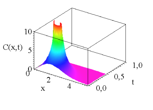
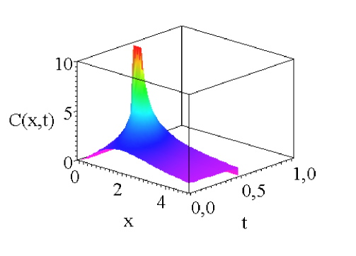
$\alpha=+1$                                             $\alpha=+\frac{1}{2}$

Figure 5: Two solutions from the blow-up kind, with the same parameters given above.

We think that our exhaustive analysis in general helps the reader to understand the complex beauty of the solutions of PDEs especially the diffusion equation. The second aim of our study is, that these concrete results could attract the interest of the community of anomalous diffusion anomdif or anomalous transport klages ; KoChKl2005 ; KoBa2011 ; LiKrDe2018 ; GiKlSo2019 .

III Summary

After a short historical summary of diffusion we presented analytic results obtained from three different Ansätze. First from the non-classical method of group invariant method, then from the traveling profile and finally the classical self-similar Ansatz. The results evaluated from the last trial function were analyzed in details, numerous formulas are given for different $\alpha\geq 0$ self-similar exponents which all mean physically relevant decaying solutions with different temporal asymptotics. Such results might exist deeply hidden in intrinsic dynamics of certain systems. As limiting solution the $\alpha=0$ was discussed in connection with fluid evaporation. Future work is in progress to perform comparable analysis among the three mentioned trial functions for non-linear diffusion equations as well. A straightforward organic generalization is when both $\alpha,\beta$ exponents can take arbitrary real numbers, it will be shown in future studies that such cases may be related to diffusion equations which have time-dependent diffusion coefficients. Investigation of processes where the diffusion coefficients have spatial dependence is also a future challenge. This kind of in-depth similarity analysis would be desirable and instructive for second oder wave equations, too.

IV Acknowledgment

One of us (I.F. Barna) was supported by the NKFIH, the Hungarian National Research Development and Innovation Office.

References

- (1) J. Philibert, Diffusion Fundamentals 2, 1 (2005).
- (2) H. Mehrer and N.A. Stolwijk, Diffusion Fundamentals 11, 1 (2009).
- (3) Z. Wu, J. Zhao, J. Yin and H. Li Nonlinear Diffusion Equations, World Scientific, 2001.
- (4) A. Favini and G. Marinoschi, Degenerate Nonlinear Diffusion Equations, Springer, 2012.
- (5) A. Pekalski and K. Sznajd-Weron, Anomalous Diffusion, Springer, 1999.
- (6) C. Bucur and E. Valdinoci, Nonlocal Diffusion and Applications, Springer, 2016.
- (7) L.R. Evangelista and E.K. Lenzi, Fractional Diffusion Equations and Anomalous Diffusion, Cambridge University Press, 2018.
- (8) J. Crank, The Mathematics of Diffusion, Oxford, Clarendon Press, 1956.
- (9) R. Balescu, Statistical Dynamics: Matter out of Equilibrium, Imperial College Press, London, 1997.
- (10) S. Dattagupta, Diffusion Formalism and Applications, Taylor an Francis CRC Press, 2014.
- (11) T.D. Bennett, Transport by Advection and Diffusion: Momentum, Heat and Mass Transfer, John Wiley & Sons, Hoboken, NJ, 2013.
- (12) R.B. Bird, W.E. Stewart, E.N. Lightfoot and D.J. Klingenberg, Introductory Transport Phenomena, John Wiley & Sons, Hoboken, NJ, 2015.
- (13) F. Pasquill and F.B. Smith, Atmospheric Diffusion, Ellis Horwood Limited, West Sussex, 1983.
- (14) G.T. Csanady, Turbulent Diffusion in the Environment, D. Reidel Publishing Company, 1973.
- (15) P. Neogi, Diffusion in Polymers, Marcel Dekker Inc, 1996.
- (16) J. Janssen, O. Manca and R. Manca, Applied Diffusion Processes from Engineering to Finance, John Wiley & Sons, Inc., 2013.
- (17) P. Shakarian, A. Bhatnagar, A. Aleali, E. Shaabani and R. Guo, Diffusion in Social Networks, Springer, 2015.
- (18) J. Machta and R. Zwanzig, Phys. Rev. Lett., 50, 1959 (1983).
- (19) I. Claus and P. Gaspard, Phys. Rev. E 63, 036227 (2001).
- (20) P. Gaspard, G. Nicolis and J. R. Dorfman, Physica A 323, 294 (2002).
- (21) L. Mátyás, T. Tél and J. Vollmer, Phys. Rev. E 69, 016205 (2004).
- (22) L. Mátyás and P. Gaspard, Phys. Rev. E 71, 036147 (2005).
- (23) L. Mátyás and R. Klages, Physica D 187, 165 (2004).
- (24) R. Klages, I.F. Barna and L. Mátyás, Physics Letters A 333, 79 (2004).
- (25) L. Mátyás and I.F. Barna, Chaos, Solitons and Fractals 44, 1111 (2011).
- (26) A. Halev and D.M. Harris, Chaos 28, 096103 (2018).
- (27) D. Ando, N. Korabel, K.C. Huang and A. Gopinathan, Biophysical Journal 109, 1574 (2015).
- (28) T. Panda, Bioreactors Analysis and Design, Tata McGraw Hill, New Delhi, 2015.
- (29) D. Iftimie, SIAM J. Math. Anal. 33, 1483, (2002)
- (30) X.R. Hu, Z.Z. Dong, F. Huang, et al., Z. Naturforschung A 65, 504 (2010).
- (31) X.Y. Jiao, Communications in Theoretical Physics 52, 389 (2009).
- (32) K. Fakhar, T. Hayat, C. Yi and N. Amin, Communication in Theoretical Physics. 53, 575 (2010).
- (33) I.F. Barna, Communications in Theoretical Physics 56, 745 (2011).
- (34) L.H. Yeung and M. Yuen., Proceedings of the American Mathematical Society 139, 3951 (2011).
- (35) I.F. Barna and L. Mátyás, Fluid Dynamics Research 46, 055508 (2014).
- (36) H.Y. Wu, J.X. Fei and C.L. Zheng, Communication in Theoretical Physics 54, 55 (2010).
- (37) C. Dai, Y. Wang and C. Yan, Optics Communications 283, 1489 (2010).
- (38) Y. Gao and S.Y. Lou, Communication in Theoretical Physics 52, 1031 (2009).
- (39) M. Nagasawa, Schrödinger Equations and Diffusion Theory, Springer, 1993.
- (40) R. Aebi, Schrödinger Diffusion Processes, Birkhäuser Verlag, 1996.
- (41) S. Kakac, Y. Yener and C.P. Naveira-Cotta Heat Conduction, CRC Press Taylor & Francis Group, 2018.
- (42) D.W. Hahn and M.N. Özisik, Heat Conduction, John Wiley & Sons, Inc., 2012.
- (43) D.D. Joseph and L. Preziosi, Rev. Mod. Phys. 62, 375 (1990).
- (44) E. Kovács, Numer. Methods Partial Differ. Eq. 37, 2469 (2020).
- (45) E. Kovács, J. Comput. Appl. Mech. 15, 3 (2020).
- (46) I.F. Barna and R. Kersner, J. Phys. A: Math. Theor. 43, 375210 (2010).
- (47) R. Garra, E. Orsingher and E.L. Shishkina, Lobachevskii Journal of Mathematics, 40, 640 (2019).
- (48) I.F. Barna and R. Kersner, Journal of Generalized Lie Theory and Applications 10, S2 (2016).
- (49) G. Ben-Dor O. Igra and O. Sadot, Editors 30th International Symposium on Shock Waves ISSW30 Conference Proceedings Springer 2017 - Volume 2, I.F. Barna and R. Kersner, Heat Conduction: Hyperbolic Self-Similar Shock-Waves in Solids, Page 927 - 931.
- (50) A.W. Liehr, Dissipative Solitons in Reaction Diffusion Systems: Mechanisms, Dynamics, Interaction , Springer Series in Synergetics 7, 2013.
- (51) B.H. Gilding and R. Kersner, Travelling Waves in Nonlinear Diffusion-Convection Reaction, Birkhäuser Basel, 2004.
- (52) Y. Mahmoudi, K. Hooman and K. Vafai (Editors), Convective Heat Transfer in Porous Media, CRC Press, 2019.
- (53) A.-L. Barabási and H. E. Stanley, Fractal concepts in surface growth, Press Syndicate of the University of Cambridge, 1995.
- (54) Y. Povstenko, Linear Fractional Diffusion-Wave Equation for Scientists and Engineers, Birkhäuser Basel, 2015.
- (55) D. Ricciotti, P-Laplace equation in the Heisenberg group: regularity of solutions, Springer Briefs in mathematics, 2016.
- (56) G. Bognár, E. J. Qualitative Theory of Diff. Equ., 4, 1 (2008).
- (57) H.S. Carslaw and J.C. Jaeger, Conduction of Heat in Solids, Oxford: Clarendon Press, 1959.
- (58) J. Mathews and R.L. Walker, Mathematical methods of physics, New York: W. A. Benjamin, 1970.
- (59) R.K.M Thambynayagam, The Diffusion Handbook: Applied Solutions for Engineers, McGraw-Hill, 2011.
- (60) G.W. Bluman and J.D. Cole, J. Math. Mech., 18, 1025 (1969).
- (61) P.A. Clarkson and M.D. Kruskal, Journal of Mathematical Physics, 30, 2201 (1989).
- (62) N. Benhamidouche, J. Qual. Theory Diff. Equat. 15, 1 (2008).
- (63) L. Sedov, Similarity and Dimensional Methods in Mechanics, CRC Press, 1993.
- (64) Ya.B. Zel’dovich and Yu. P. Raizer Physics of Shock Waves and High Temperature Hydrodynamic Phenomena Academic Press, New York, 1966.
- (65) G.I. Baraneblatt, Similarity, Self-Similarity, and Intermediate Asymptotics Consultants Bureau, New York 1979.
- (66) D. Campos editor, Handbook on Navier-stokes equations. Theory and Applied Analysis. Chapter 16, I.F. Barna ”Self-similar analysis of various Navier-stokes equations in two or three dimensions. Pages 275 - 304 Publishers, New York, 2017.
- (67) I.F. Barna, Laser Phys. 24, 086002 (2014).
- (68) I.F. Barna, M.A. Pocsai and L. Mátyás, Journal of Generalized Lie Theory and Application 11, 1000271 (2017).
- (69) G.Nath and S. Singh, Journal of Astrophysics and Astronomy 40, 50 (2019).
- (70) P.K. Sahu, Brazilian Journal of Physics 50, 548 (2020).
- (71) C. Kanchana, Y. Su and Y. Zhao, Communications in Nonlinear Science and Numerical Simulation 83, 105129 (2020).
- (72) I.F. Barna. M.A. Pocsai, S. Lökös and L. Mátyás, Chaos, Solitons and Fractals 103, 336 (2017).
- (73) F.W.J. Olver, D.W. Lozier, R.F. Boisvert and C.W Clark, NIST handbook of mathematical functions, Cambridge University Press, 2010.
- (74) D. N. Gerasimov and E. I. Yurin, Kinetics of Evaporation, Springer, 2018.
- (75) W. Deng, R. Hou, W. Wang and P. Xu Modeling Anomalous Diffusion: From Statistics to Mathematics, World Scientific Publishing Company, 2020.
- (76) Edited by R. Klages, G. Radons and I. M. Sokolov Anomalous Transport, Foundations and Applications, WILEY-VCH Verlag GmbH & Co. KGaA 2008.
- (77) N. Korabel, A.V. Chechkin, R. Klages, I.M., Sokolov and V.Yu. Gonchar, Europhysics Letters 70, 63 (2005).
- (78) N. Korabel and E. Barkai, Physical Review E 83, 051113 (2011).
- (79) A.L Livorati, T. Kroetz, C.P. Dettmann, I.L. Caldas, and E.D. Leonel, Physical Review E 97, 03220 (2018).
- (80) S. Gil-Gallegos, R. Klages, J. Solanpää and E. Räsänen, The European Physical Journal Special Topics 228, 143 (2019).