Causal Program Dependence Analysis

Abstract.

We introduce Causal Program Dependence Analysis (CPDA), a dynamic dependence analysis that applies causal inference to model the strength of program dependence relations in a continuous space. CPDA observes the association between program elements by constructing and executing modified versions of a program. One advantage of CPDA is that this construction requires only light-weight parsing rather than sophisticated static analysis. The result is a collection of observations based on how often a change in the value produced by a mutated program element affects the behavior of other elements. From this set of observations, CPDA discovers a causal structure capturing the causal (i.e., dependence) relation between program elements. Qualitative evaluation finds that CPDA concisely expresses key dependence relationships between program elements. As an example application, we apply CPDA to the problem of fault localization. Using minimal test suites, our approach can rank twice as many faults compared to SBFL.

1. Introduction

Program dependence analysis is a fundamental task in software engineering. In addition to being the foundation of program comprehension (Zhifeng Yu and Rajlich, 2001), program dependence analysis underlies various software engineering tasks, including software testing (Binkley, 1997), debugging (Jiang et al., 2017; Lee, 2020), refactoring (Ettinger and Verbaere, 2004), maintenance (Gallagher and Lyle, 1991), and security (Karim et al., 2018). It often supports these tasks by reducing the number of program elements that must be considered.

Each component of a program depends, to some degree, on the other components of the program. Some of these dependence relations are strong, i.e. a change in one component almost surely changes the value of another, while others are weaker. Traditional static dependence analysis attempts to safely approximate all possible dependence relations. This can become quite involved, and will return many relations. A good example would be pointer analysis, which is not only computationally expensive but also prone to produce a large number of dependence relations including many false positives. Furthermore, static analysis typically does not attempt to estimate the strength of a dependence. Thus its output is a large number of equally-weighted dependencies, which tends to degrade the ability of a developer to work with the code based on the results of the analysis. A few dynamic dependence analysis approaches have modeled dependence strengths (Baah et al., 2010; Yu et al., 2017), but they are typically built on top of (expensive) static dependence analysis (e.g., the construction of a Program Dependence Graph), and remain vulnerable to confounding bias due to their formulation based on conditional probability, which captures mere association, rather than causation (Baah et al., 2010; Yu et al., 2017; Lee et al., 2019).

This paper proposes Causal Program Dependence Analysis (CPDA), a framework that analyzes the degree (or strength) of the dependence between program elements. Given a set of executions, CPDA makes use of associations between observed behavior of program elements to discover a causal structure. By applying techniques for causal inference (Pearl, 2009; Pearl et al., 2009), over this causal structure, CPDA then produces two measures of program dependence: causal dependence and direct dependence. Causal dependence aggregates the effect that a change at a program element has on the behavior of other program elements. A direct dependence is the effect of one program element on another, excluding any effects that pass through other elements.

One advantage of CPDA is that it does not require extensive “heavy weight” static analysis. Instead, only light-weight parsing of the source code, or light-weight instrumentation of a binary, is required. Essential points of interest in the code are annotated so we can introduce simple mutations to the state, and observe their effects using a set of test inputs. An additional benefit is thus that our approach can be applied to heterogeneous systems built from multiple languages, as long as a parser (or method for instrumenting binary representations) is available.

To evaluate CPDA, we first build a Causal Program Dependence Model (CPDM), and then introduce and study its use for Causal Dependence based Fault Localization (CDFL). The CPDM is a graph in which we annotate the direct dependence on the causal structure to represent a program’s dependences. We investigate how well the (strength of the) direct dependence captures the program’s semantics. We also consider how characteristics of the test suite impacts the resulting CPDM.

To further study the utility of CPDA, we propose Causal Dependence based Fault Localization (CDFL), which calculates the suspiciousness of program elements in light of failing test cases, based on CPDA. We evaluate CDFL using the Siemens suite, a well-known benchmark for testing and debugging. Compared to Spectrum based Fault Localization (SBFL) (Naish et al., 2011; Xie et al., 2013), our empirical results CDFL can rank 166% more actually faulty program elements at the top.

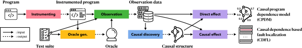
Framework of Causal Program Dependence Analysis

Figure 1. Framework of CPDA

The main contributions of this paper include the following:

• We propose Causal Program Dependence Analysis. This dependence analysis framework, based on causal inference, supports the quantification of dependence strength among program elements.

• We present an illustrative example where quantifiable program dependence enables us to visualize program semantics and the effect of different inputs on them.

• To illustrate the utility of CPDA, we introduce Causal Dependence based Fault Localization (CDFL). Our empirical evaluation of CDFL shows that it outperforms existing fault localization techniques, especially in challenging cases that other techniques find difficult.

The rest of this paper is organized as follows. We first describe CPDA, starting with an introduction of causal inference in Section 2. Section 3 describes the design of our empirical evaluation, the results of which are presented in Section 4. Section 5 discuss the remaining challenges in CPDA and presents future work. Threats to validity are discussed in Section 6. Finally, we review related work in Section 7, and conclude in Section 8.

2. Causal Program Dependence Analysis (CPDA)

This section first introduces causal inference in general, and subsequently presents a detailed explanation of our framework, Causal Program Dependence Analysis (CPDA).

2.1. Causal Inference

Causal inference is a fundamental, mathematical theory for analyzing which factors cause one or more effects (Pearl, 2009; Pearl et al., 2009). While statistical methods focus on identifying and modeling associations, causal analysis adds ways of studying which factors actually precede and leads to (causes) changes in others, and how large their effects are. Such an analysis can provide practical benefits and ultimately lead to more robust solutions. As an example, in medicine, a reanalysis of data on hip fractures among the elderly (Caillet et al., 2015) found that the causal analysis was able to identify which factors mediate the effect of the others and to what extent, in addition to providing predictions on par with traditional methods. In another study, Richens et al. (Richens et al., 2020) showed that medical diagnosis based on causal inference performed almost twice as good (25th percentile vs. 48th of the performance of human doctors) as the classical, associative/statistical method.

A key element of causal inference is to use directed acyclic graphs (DAGs) to model the observed factors’ dependence structure. Nodes in the graph denote factors, and edges denote ways that (parent) variables cause changes in other (child) factors. The DAG of a causal model thus makes the causal dependence structure explicit. In addition to the DAG, a causal model includes a way to estimate child factors based on the values of their parent(s). In a so called structural equation model, this is achieved via equations, typically linear but more general forms can be used, that relate each child factor to the nodes from which is has incoming DAG edges. Another model variant, the probabilistic causal model, uses a single probability distribution over the factors (Pearl, 2009). While the causal structure, i.e., the DAG, is sometimes known or can be formulated from a theory, it is more common to use so called structural learning (also called causal discovery) to identify the causal structure from data (Spirtes and Zhang, 2016). Structural learning methods can either work only from observational data or also (or solely) use interventional data, i.e. when we have taken actions that lead to changed values for some subset of factors of a DAG. A hallmark of causal analysis is that its DAGs can be used both to guide which factors to intervene on, i.e. change, and then tell us how to calculate the causal effects from our observations.

2.2. Overview of CPDA

Causal Program Dependence Analysis (CPDA) aims to model and quantify the strength of program dependence relations. The dependence reported by CPDA is thus not binary: rather, it represents how likely a change to the value of a program element $S_{i}$ is to cause a change to the value of another element $S_{j}$. To capture the causal relations between program elements, we initially capture the behavior of the original program when executed on a test suite, to use as oracle. We then observe whether systematically mutated program variants behave differently to the oracle. Technically, we let the change status of a program element be a random variable in causal inference. Our causal inference thus uses both purely observational data, the behavior of the unmutated program, as well as interventional data, the behaviors of the mutated program variants.

Figure 1 shows the overall framework of CPDA. Given a program, CPDA identifies target program elements to analyze, and subsequently mutates and instruments the code (Sec. 2.3). The instrumentation allows us to generate an oracle, a set of recorded behaviors, i.e. states of variables, of the original, unmutated program. Super-mutation allows us to apply interventions to the program elements and monitor the resulting changes (Untch et al., 1993). Using these observations (Sec. 2.4), CPDA builds a causal structure (Sec. 2.5) and performs causal inference to calculate the causal and the direct dependence (Sec. 2.6). We also introduce Causal Dependence based Fault Localization (CDFL), a novel fault localization technique based on CPDA. Using causal dependence, we try to identify the program element that is the most likely to cause the observed failure (Sec. 2.7).

2.3. Instrumentation, Oracle, and Mutation

We mutate and instrument the target program simultaneously, so that we can apply intervention to the behavior of the original program and observe its impact. Given a program, let a node correspond to each left-hand side variable that occurrs in assignment statements, function parameters, predicates, and return values of functions: we use the term “node” because CDPA eventually will represent all these program elements as nodes in the graph of a causal model. Given a node, its trajectory represents the behavior of the node, i.e. the sequence of values it takes during execution.

2.3.1. Instrumentation

A pair consisting of an intervention and the measurement of its impact is called an observation. To efficiently produce a large and diverse set of observations for program $P$, we construct a super mutant (Untch et al., 1993), i.e., a meta-mutated program that takes a mutation position (a unique index of each node), and a mutation value that will be used whenever the node is executed, as input: this reduces the number of compilations required for multiple mutations. The instrumentation begins by indexing all the nodes in the target program using a parser, and injecting a helper function. The helper function, when given a target node index, will overwrite (i.e., mutate) the value of the node, and log the result of mutation, during execution. For all the other nodes, the helper function simply logs their current value observed during execution (i.e., record their trajectories).

2.3.2. Oracle

Once the target program is instrumented, we can obtain the oracle for each node using the given test suite. An oracle for a node is simply a collection of all of its trajectories, one per a test input in the test suite, when no mutations are active during execution.

2.3.3. Mutation

CPDA currently targets primitive variables of the following types: bool, char, int, long, float, double, and string. For booleans, we mutate by simply negating the original value. For primitive types, we sample a random value from a Gaussian distribution that is based on all observed values in its trajectories. However, when the domain knowledge clearly specifies the range of possible values (such as an input parameter that can be only 0, 1, or 2), we simply sample from the given range with a uniform probability. Finally, for strings, we first sample the string length from a Gaussian distribution that is based on the length of all observed strings for the node, and subsequently sample a random lowercase string of that length. We sample the value mutation up to $N_{mpn}$ times per node. We leave more refined data mutation and generation strategies for future work and note that techniques for test generation can likely be of use as well as able to handle more complex, structured data types (Feldt and Poulding, 2013).

2.4. Representing Behavioral Changes

Once we collect the oracle (trajectories obtained by executing the original program with the given test suite) and our observations (trajectories obtained by executing the mutated programs with the given test suite), we can identify the change of program behavior due to value mutations. Formally, we define change of the behavior for a node as follows:

Definition 2.1 (Change of the behavior of a node).

Behavior of node $S_{i}$ in program $P$ has changed for a given mutation and an input, if the trajectory for $S_{i}$ using the mutated program $P^{\prime}$ is different from the trajectory of $S_{i}$ using $P$.

From now on, let us overload the notation $S_{i}$ to represent both the node itself and the variable denoting whether the behavior of $S_{i}$ has changed under $P^{\prime}$ or not; $S_{i}=1$ if changed, 0 otherwise. For a fixed mutated version $P^{\prime}$ and an input, we get a single observation, which is a boolean vector whose length is equal to the number of nodes in the program: each value in the observation indicates whether the behavior of the corresponding node has changed or not. Given a set of observations, we can calculate the probability of a node changing its behavior.

Definition 2.2 (Probability of the behavior change).

Given Node $S_{i}$ from Program $P$ and a set of observations $O$, $P_{O}(S_{i}=1)$ represents the probability of a change in $S_{i}$’s behavior, given $O$, is:

$$P_{O}(S_{i}=1)=1-P_{O}(S_{i}=0)=\frac{\left|\left\{\mathit{obs}\in O\mid\mathit{obs}[S_{i}]=1\right\}\right|}{\left|O\right|}\,.$$

Moreover, we can also express the conditional probability of node $S_{j}$ changing its behavior given that node $S_{i}$ has changed its behavior:

Definition 2.3 (Conditional probability of the behavior change).

For a given set of observations, $O$, behavior, and $O^{*}=\{o\mid o\in O\land$ node $S_{j}$ is not mutated in the mutated program that generates $o\}$:

$$\begin{split}P_{O}(S_{j}=1\mid S_{i}=1)&=\frac{P_{O}(S_{j}=1\land S_{i}=1)}{P_{O}(S_{i}=1)}\\ &=\frac{\left|\left\{\mathit{obs}\in O^{*}\mid\mathit{obs}[S_{j}]=1\land\mathit{obs}[S_{i}]=1\right\}\right|}{\left|\left\{\mathit{obs}\in O^{*}\mid\mathit{obs}[S_{i}]=1\right\}\right|}\,.\end{split}$$

The conditional probability in Definition 2.3 becomes the foundation of causal dependences that we calculate later. We exclude the mutation on $S_{j}$ itself, hence $O^{*}$, when calculating the conditional probability $P_{O}(S_{j}=1\mid S_{i}=1)$ . This is to avoid negating the effect from the change of $S_{i}$ with a mutation of $S_{j}$ itself.

Each node can have up to $N_{mpn}$ mutated values (see Section 2.3). Since each node may have a different number of mutated values, we normalize the probabilities in Def. 2.2 and 2.3 by multiplying the reciprocal of the number of sampled mutated values. For example, each observation for an integer type node mutation from ten mutation values has a weight of 0.1.

2.5. Causal Structure Discovery

The conditional probability defined in Def. 2.3 expresses the association between changes of program elements: changes are simply observed together. To elevate this to causal inference, we need the concept of a specific change preceding another. It is also necessary to distinguish between direct predecessors, i.e., nodes whose change directly affects our target node, and non-direct predecessors, i.e., nodes whose change does affect our target node but indirectly through one or more direct predecessors.

A causal structure allows us to introduce this concept of precedence. Program dependence is inherently a form of causal precedence: if node $S_{j}$ depends on node $S_{i}$, a change in $S_{i}$ will precede the change in $S_{j}$. Consequently, in principle, a perfectly accurate PDG of the target program can serve as a causal structure, if available. However, in reality, existing dependence analysis is both computationally costly and may not be accurate. Instead, we use ideas from the causal inference field and approximate the causal structure from the set of observations we have collected.

Let us first formally define the predecessors of a node. We identify the predecessors of a node $S_{j}$ by checking whether intervening on a particular node affects $S_{j}$. We call predecessors of a node as its intervention parents.

Definition 2.4 (Intervention Parent).

For a program $P$ and a set of nodes $S$ from the program, a set of nodes $\mathit{IPA}_{j}\subset S$ is said to be intervention parents of $S_{j}$ if mutating any node in $\mathit{IPA}_{j}$ changes the behavior of $S_{j}$ for at least one input. In other words, if a mutated program $P^{\prime}$ that changes the value of $S_{k}$ to $v$ causes $S_{j}=1$ under input $i$, then $S_{k}\in\mathit{IPA}_{j}$.

However, the precedence relationship may be direct, or indirect (i.e., a change in one of the intervention parents will, by definition, precede the change in the child node, but its effect may or may not need to pass through another parent to affect the child node). Based on the theory of causal inference, we define Markovian parents of a node as the minimal set of direct predecessors among the intervention parents.

Definition 2.5 (Markovian parent).

The Markovian parents of $S_{j}$, $\mathit{PA}_{j}$, is a minimal set predecessors of $S_{j}$ that renders $S_{j}$ independent of all its intervention parents. In other words, $\mathit{PA}_{j}$ is any subset of $\mathit{IPA}_{j}$ such that it satisfies $P(s_{j}\mid\mathit{pa}_{j})=P(s_{j}\mid\mathit{ipa}_{j})$ while no other proper subset of $\mathit{PA}_{j}$ does.

Subsequently, the Markovian parent-child relation constructs the causal structure of the program.

Definition 2.6 (Causal structure).

The causal structure of a program represents the Markovian relation between the nodes. The causal structure is represented by a graph, $G=(V,E)$, where $V=\left\{S_{i}\right\}_{i\in{1..n}}$ and $E=\left\{\left(S_{i},S_{j}\right)\mid S_{i}\in\mathit{PA}_{j}\right\}$, where $\mathit{PA}_{j}$ denotes Markovian parents of $S_{j}$.

Input: $\mathit{IPA}_{j}$: Intervention parents of $S_{j}$,
$Dist$: Ordered nodes considering the distance from $S_{j}$,
$O$: Observations generated from inputs that cover $S_{j}$ in the original program.

Output: $\mathit{PA}_{j}$: Markovian parents of $S_{j}$

1 $\mathit{PA}_{j}\leftarrow\{\}$

2 $Cand\leftarrow\mathit{IPA}_{j}$

3 while $Cand.len()\neq 0\land Cand\neq\mathit{PA}_{j}$ do

4       $Remain\leftarrow Cand\setminus\mathit{PA}_{j}$

5       $S_{d}\leftarrow Dist.getFarthest(Remain)$

6       if $Cand.len()==1$ then

7             if $P_{O}(S_{j}=1\mid S_{d}=0)=P_{O}(S_{j}=1\mid S_{d}=1)$ then

8                   $is\_parent\leftarrow False$

9            else  $is\_parent\leftarrow True$

10            

11      else

12             $S_{other}\leftarrow Cand\setminus S_{d}$

13             $is\_parent\leftarrow False$

14             foreach $s_{other}\in O|_{S_{other}}$ do

15                   if $P_{O}(S_{j}=1\mid S_{d}=0,s_{other})\newline \neq P_{O}(S_{j}=1\mid S_{d}=1,s_{other})$ then

16                         $is\_parent\leftarrow True$

17                         break

18                  

19            

20      if $is\_parent$ then  $\mathit{PA}_{j}.add(S_{d})$

21       else

22             $Cand.remove(S_{d})$

23             $\mathit{PA}_{j}\leftarrow\{\}$

24      

return $\mathit{PA}_{j}$

Algorithm 1 Generate Markovian parents from $\mathit{IPA}$

It requires an exponential number of computations to compute the conditional probability in Def. 2.5 for every possible combination of intervention parents. Thus, we approximate the Markovian parents by iteratively removing non-Markovian parents from intervention parents. Algorithm 1 shows the process of removing non-Markovian parents from $\mathit{IPA}_{j}$. We choose one node $S_{d}$ from $\mathit{IPA}_{j}$ and check whether $S_{j}$ is independent from $S_{d}$, given all other candidate nodes.

If $S_{d}$ is the only candidate node left (Line 7-9), we check whether $S_{j}$ is independent from $S_{d}$. If it is, $S_{d}$ is not a Markovian parent, otherwise, $S_{d}$ is not a Markovian parent. If there are other candidate nodes $S_{other}$ (Line 11-16), we check the conditional independence of $S_{j}$ from $S_{d}$ for every realization of $S_{other}$. If $S_{j}$ is conditionally independent from $S_{d}$ for all $s_{other}$, $S_{d}$ is not a Markovian parent. Otherwise, $S_{d}$ could be a Markovian parent of $S_{j}$. This is because $S_{j}$ can be conditionally independent from $S_{d}$ if $S_{other}$ changes. Therefore, we re-check all possible Markovian parents every time we find a new non-Markovian parent. To minimize re-checking cost, we order the candidate nodes ($Dist$) to choose the most unlikely to be the Markovian parent first (Line 5). Our intuition is that, during the execution of the program, the node executed earlier than the execution of $S_{j}$ is less likely to be a parent of $S_{j}$. Algorithm 1 approximates Markovian parents of a node, as it only considers individual nodes, and not their combination, for Makovian parents.

The last step of building a causal structure is to eliminate cycles in the structure. In causal inference, the form of the causal structure is the Bayesian network, which has no cycles. To eliminate cycles, we remove from $S_{i}$ in $\mathit{PA}_{j}$ if $S_{j}$ is in $\mathit{IPA}_{i}$.

2.6. Causal Program Dependence Model

We first introduce causal dependence, which measures the total effect of each node’s change that causes a change in another node, and subsequently introduce direct dependence, which measures the effect of one node on another excluding all the (indirect) effects through other nodes.

2.6.1. Causal dependence

The conditional probability $P(\cdot|x)$ represents the probability when one observes that $X$ has value $x$. By having a causal structure, we can instead estimate the probability when we force $X$ to have the value $x$, denoted as $P(\cdot|do(x))$. The difference between ”forcing” and ”observing” comes from whether and how the effect of $X$ is affected by other nodes. A confounding bias, a distortion representing the event that is associated but not casually related to the observation, appears through the so-called backdoor path in a causal DAG (Pearl, 2009). By ignoring the incoming effect of $X$, we can remove the effect through the backdoor path to $X$, subsequently eliminating the confounding bias from the association between $X$ and another node $Y$. Note that backdoor paths in CPDM are based on the inferred causal structure, unlike existing work (Baah et al., 2010) Based on Pearl et al. (Pearl, 2009), the causal effect estimating $P(\cdot|do(x))$ is formally defined below: we use a set of nodes, instead of a single node, to include the more general scenario where multiple nodes are mutated simultaneously.

Definition 2.7 (Causal Effect).

Let $G=(V,E)$ be a causal structure. Given two disjoint sets of nodes, $X,Y\subset V$, the causal effect of $X$ on $Y$, denoted either as $P(y\mid\hat{x})$ or $P(y\mid do(x))$, is a function from $X$ to the space of probability distributions on $Y$. For each realization $x$ of $X$, $P(y\mid\hat{x})$ gives the probability that $Y=y$ induced by deletion from the causal structure of all the edges to nodes in $X$ other than $x$ and thus considering $X=x$. The causal effect $P(y\mid do(x))$ is calculated as:

$$P(y\mid do(x))=\sum_{pa_{X}}P(y\mid x,pa_{X})P(pa_{X})\,,$$

where $PA_{X}$ represents the Markovian parents of $X$.

In causal program dependency analysis, we aim to measure the amount of impact that the change of one node $S_{i}$ has on another node $S_{j}$, i.e., the difference between the causal effect from “$S_{i}=1$” to $S_{j}$, and from “$S_{i}=0$” to $S_{j}$. Thus, we introduce causal dependence as follows:

Definition 2.8 (Causal Dependence).

The causal dependence of node $S_{i}$ to $S_{j}$ measures how much changing the behavior of $S_{i}$ affects the behavior of node $S_{j}$. Given a set of observations $O$, the causal dependence of $S_{i}$ to $S_{j}$, $\mathit{CD}_{O}(S_{i},S_{j})$, is defined as:

$$\mathit{CD}_{O}(S_{i},S_{j})=P_{O}(S_{j}=1\mid do(S_{i}=1))-P_{O}(S_{j}=1\mid do(S_{i}=0))\,.$$

2.6.2. Direct dependence

Direct dependence quantifies the amount of effect that is not mediated by, any other nodes. More formally, it measures the sensitivity of $Y$ to changes in $X\in\{$Markovian parents of $Y\}$ while all other Markovian parents of $Y$ are held fixed. Based on Pearl et al. (Pearl, 2009), a generic definition that fits such sensitivity is the natural direct effect.

Definition 2.9 (Natural Direct Effect).

The natural direct effect, denoted either as $\mathit{NDE}_{X:x\rightarrow x^{\prime}}(Y)$ is the expected change in $Y$ induced by changing $X$ from $x$ to $x^{\prime}$ while keeping all mediating factors constant at whatever value they would have been under $do(x)$. The natural direct effect, $\mathit{NDE}_{X:x\rightarrow x^{\prime}}(Y)$, is calculated as:

$$\sum_{z}\left[E\left(Y\mid do(x^{\prime},z)\right)-E\left(Y\mid do(x,z)\right)\right]P\left(z\mid do(x)\right),$$

where $Z$ represents all parents of $Y$ excluding $X$.

Similar to causal dependence, in the context of CPDA, we estimate how much effect a parent has on a child node $S_{j}$ when the parent node $S_{i}$ alter from “unchanged” to “changed”, regardless of all other parents of $S_{j}$. Based on the definition of the natural direct effect, we define the direct dependence as follows.

Definition 2.10 (Direct Dependence).

The direct dependence of $S_{j}$ from $S_{i}$, denoted as $\mathit{DD}_{I}(S_{i},S_{j})$, is the average of the natural direct effect of $S_{i}$ towards $S_{j}$ over all inputs $I$:

$$\mathit{DD}_{I}(S_{i},S_{j})=\frac{1}{|I|}\sum_{t\in I}\mathit{NDE}_{O_{t},S_{i}:0\rightarrow 1}(S_{j})\,,$$

where $O_{t}$ denotes the observations from input $t$, and $\mathit{NDE}_{O_{t},S_{i}:0\rightarrow 1}(S_{j})$ denotes the natural direct effect using the observations $O_{t}$.

2.6.3. Causal Program Dependence Model

Given the definition of the direct dependence, CPDM is a weighted dependence graph of the program. Its structure is the causal structure, and the edge’s weight, indicating the strength of dependence, is the direct dependence between the nodes. CPDM is thus a novel graph representation to explain program dependence in a continuous, gradual way.

2.7. Causal Dependency Based Fault Localization

CPDA allow us to compare the relative strengths of different dependency relationships in a program. To highlight the benefits of this quantification, we propose Casual Dependence based Fault Localization (CDFL). The main hypothesis of CDFL is that the faulty program element, that we are trying to locate, will have more impact on the output element in failing executions than in passing executions. This is intuitive since the basic assumption in fault localization is that there is a faulty element that is causing the faulty output; if it is faulty but is not causing this particular fault we are (currently) not looking for it. The ability to compare the strength of different dependence relationships means that we can rank program elements according to their effect on the faulty output. This is not possible in fault localisation techniques based on binary program dependence, such as dicing (Agrawal and Horgan, 1990).

Given an output node $S_{out}$ which causes the test failure, we can compute the suspiciousness score of node $S_{i}$, $susp(S_{i})$, as:

$$\frac{1}{|I_{fail}|}\sum_{t\in I_{fail}}\mathit{CD}_{O_{t}}(S_{i},S_{out})-\frac{1}{|I_{pass}|}\sum_{t\in I_{pass}}\mathit{CD}_{O_{t}}(S_{i},S_{out}),$$

where $I_{fail}$ and $I_{pass}$ denote a set of failing and passing test inputs, respectively. Note that the value of $S_{out}$ represents the change of outcome, and not pass or fail.

Table 1. Example comparing CDFL to SBFL

Code	Rank${}_{\text{SBFL}}$	Rank${}_{\text{CDFL}}$
a = 3	1	2
b = 4	1	3
c = a % 3 + 1	1	1
return c	-	-

2.7.1. Advantages over SBFL

Table 1 contains a motivating example showing the advantages of CDFL over SBFL: the fault is typeset in red. SBFL assigns suspiciousness scores to program elements based on the coverage and outcomes of test executions (Wong et al., 2016). Consequently, its performance depends significantly on the differences in control flow between passing and failing executions: it fails to distinguish the failing execution in Table 1, which can be only characterized in data flow. Moreover, all statements in the same program block are assigned with the same suspiciousness score, as can be seen in the example. CDFL, however, can correctly analyze that the faulty return value is caused by the assignment to variable c.

Table 2. Example comparing CDFL to Dynamic Slicing and Dicing. ‘␣’ denotes the whitespace.

Code	Coverage			DS	Dice	Susp${}_{\text{CDFL}}$
	“a”	“a␣”	“␣a␣”
s = input()	1	1	1	1	0	1.0 - 1.0 = 0.0
pred = isEndSpace(s)	0	1	1	1	0	1.0 - 0.5 = 0.5
if (pred) p = p.rstrip() p.strip()	0	1	1	1	0	1.0 - 0.5 = 0.5
return p	-	-	-	-	-	-
Test Results	P	P	F

2.7.2. Advantages over Dynamic Slicing and Dicing

Table 2 contains a motivating example showing the advantages of CDFL over DS, a dynamic backward slice of the returned variable p, and a dice (Agrawal et al., 1995), which essentially returns the set difference between dynamic slices computed using failing test inputs and passing test inputs. Intuitively, if there is a dependence relationship that is only exercised in failing executions, dicing reports it as the likely root cause of the failure. The original code in Table 2 intends to only remove trailing whitespaces (denoted as ‘␣’), but the faulty version strips all whitespaces. Because one of the passing inputs, “a␣”, and the failing input, “␣a␣”, execute all lines of the code, dynamic slicing reports all lines to be equally faulty, while dicing concludes that none of them are faulty. However, CDFL reports that the faulty line is more suspicious, based on the quantitative dependence.

3. Experimental Setup

This section presents our research questions and the set-up of our empirical evaluation.

3.1. Research Questions

CDFL is but one possible use of the general program dependence analysis method of CPDA. In addition to evaluating CDFL, we thus first ask a more general research question about CPDA.

RQ1. Effectiveness of CPDA: How well does CPDA capture the relative strengths of dependence between program elements? We expect the direct dependence to capture the varying degrees of dependence between program elements. To investigate this, we build CPDMs for an example program with well known dependencies, and examine how it differs from PDG. We also investigate its sensitivity when using different test suites.

RQ2. Performance of CDFL: How well does CDFL perform compared to other, widely studied fault localisation techniques? We evaluate the utility of CPDA through CDFL, by comparing the fault localisation results to Spectrum Based Fault Localization (SBFL), dynamic slicing, and dicing. We also investigate the impact that the number of observations, $N_{mpn}$, has on the accuracy of CDFL.

3.2. Subjects and Baselines

This section describes the subject programs, and baseline techniques, for the CPDA (RQ1) and CDFL (RQ2) study, respectively.

3.2.1. CPDA Study (RQ1)

⬇

1def main() {

2 <1>characters = 0

3 <2>lines = 0

4 <3>words = 0

5 <4>inword = 0

6 <5>_pred1 = getChar(<6>c)

7 while (_pred1) {

8 <7>characters = characters + 1

9 <8>_pred2 = c == ’\n’

10 if (_pred2)

11 <9>lines = lines + 1

12 <10>_pred3 = isLetter(c)

13 if (_pred3) {

14 <11>_pred4 = inword == 0

15 if (_pred4) {

16 <12>words = words + 1

17 }

⬇

18 <13>inword = 1

19 }

20 else

21 <14>inword = 0

22 <15>_pred1 = getChar(<16>c)

23 }

24}

25def isLetter(<17>c) {

26 <18>_pred5 = ((c >= ’A’ && c <= ’Z’)

27 || (c >= ’a’ && c <= ’z’))

28 if (_pred5)

29 <19>_ret = True

30 else

31 <20>_ret = False

32 return _ret

33}

Figure 2. Pseudo-code of the word count program

Pseudo-code of the word count program

To investigate RQ1, we apply CPDA to the word count (wc) program, which has been widely studied for program dependence analysis (Gallagher and Lyle, 1991; Lee et al., 2019). Figure 2 shows the pseudo-code of the word count program. The node index annotations in angled brackets are used to refer to corresponding nodes in Section 4.1. The word count program takes a text as input and counts its number of characters, lines, and words. We use a test suite of 15 test cases, which can be grouped into the following:

onechar:

: Tests 1-3 contain a single letter.

oneword:

: Tests 4-7 contain a single word of multiple letters.

oneline:

: Tests 8-10 contain a single line with multiple words.

multiline:

: Tests 11-15 contain multiple lines of multiple words.

For each node, we use a sample of 100 mutations ($N_{mpn}=100$) and observe the changes at other nodes.

Table 3. Statistics of the Siemens suite

Subject	SLoC	N${}_{\text{bug}}$	N${}_{\text{test}}$	N${}_{\text{failing test}}$	N${}_{\text{node}}$
tcas	135	34	5–7	1–1	43
schedule	292	4	8–9	1–2	94
schedule2	297	3	7–10	1–1	147
totinfo	346	18	7–10	1–4	172
printtokens	475	3	11–17	1–1	293
printtokens2	401	6	12–15	1–3	186
replace	512	24	16–20	1–2	318
total	2,458	92	-	-	1,253

(a) PDG

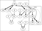
(b) $\mathit{DD}>0.2$

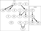
(c) $\mathit{DD}>0.8$

(d) $0.8>\mathit{DD}>0.2$

Figure 3. Program Dependence Graph (PDG) and Causal Program Dependence Models of word count with different thresholds for the Direct Dependences (DD) For CPDMs, the thicker and darker the edge is, the larger the direct dependence.

Causal Program Dependence Model of word count with different thresholds

3.2.2. CDFL Study (RQ2)

We compare CDFL to three existing FL techniques: Spectrum Based Fault Localization (SBFL), Dynamic Slicing (DS), and Dicing. As SBFL technique, we choose Ochiai (Ochiai, 1957) which is widely studied in the literature (Abreu et al., 2007).

We compute dynamic slices using the dynamic slicing algorithm of Agrawal and Horgan (Agrawal and Horgan, 1990), which intersects coverage information from a set of inputs with a static slide. We employ gcov to collect coverage information, and CodeSurfer, a static analysis tool produced by GrammaTech (Grammatech Inc., 2002), for static backward slices. Finally, we compute the dice as the difference of the dynamic slices of the failing and passing tests. Note that CDFL ranks nodes, while SBFL ranks program statements.

We compare four fault localization techniques using programs from the Siemens suite (Do et al., 2005). Table 3 provides descriptive statistics of the studied programs: columns represent Non-comment-non-blank Lines of Code (SLoC), number of studied bugs, tests, failing tests, and nodes, respectively. We randomly choose a statement coverage adequate test suite provided by SIR that contains at least one failing test for each bug.

Some of the seeded faults provided by SIR have been excluded from our study. Excluded faults can be categorized into four groups. First, we exclude omission faults, because their root causes do not exist in the given source code. Second, we exclude faults for which no failing test case exists. Third, we exclude faults that results in nondeterministic behavior, or segmentation faults, as they produce either inconsistent, or no coverage information. Finally, we exclude any fault whose root cause falls outside the scope of CPDA (for example, if the fault is calling a wrong function without storing the return value, we cannot represent the fault as a node in CPDA).

For evaluation, we use the widely adopted $acc@n$ metric, which counts the number of faults whose root causes are ranked within the top $n$ places. If there are multiple faulty elements, we compute $acc@n$ using the most highly ranked element. Since SBFL techniques tend to produce a lot of ties, we report rankings obtained by multiple tiebreakers. The average tiebreaker computes the average rank of the tied candidates. Min and max tiebreakers rank all tied elements at the highest, and the lowest, place, respectively. Finally, line order tiebreaker breaks ties independently from score distributions using line numbers, facilitating fair comparison between rankings theoretically (Xie et al., 2013).

3.3. Implementation & Environment

For node selection, we use the open source C static analyzer Frama-C (Kirchner et al., 2015). To insert logging functions in the original program, we use srcML (Collard et al., 2013), an open source tool that parses and converts source code into the XML format for manipulation.

The Markovian parent calculation (Algorithm 1) can be costly when the number of intervention parents and the number of observations are large. To reduce the cost of calculating the Markovian parents, we use safe parents ($\mathit{SPA}$), which is a subset of the intervention parents. Given $\mathit{IPA}_{j}$, the intervention parent set of $S_{j}$, the safe parent set $\mathit{SPA}_{j}$ is calculated by following heuristics:

• $\mathit{SPA}_{j}$ contains all the nodes in the same method as $S_{j}$ ($M_{j}$) or the parameters of the methods calling $M_{j}$.

• If $S_{j}$ is the left-hand side of an assignment statement, and if the assignment statement invokes the function $f$, $\mathit{SPA}_{j}$ contains the return nodes of $f$.

• If $S_{j}$ uses a global variable, $\mathit{SPA}_{j}$ contains all the nodes of the global variable.

While using the safe parent set requires an extra call graph analysis, it reduces the Markovian parent calculation time five-fold. Our experiments were performed under CentOS Linux 7, on an Intel(R) Xeon(R) CPU E5-2630 v4 with 250GB of memory.

4. Results

This section answers the research questions based on the results of our empirical investigation of CPDA.

4.1. Effectiveness of CPDM

We first consider the Causal Program Dependence Model created using the entire test suite of 15 test cases and then the four models created using the four groups. Figure 3(d) contains the PDG of wc produced manually (Fig. 3(a)), along with visualizations of three CPDMs that contain edges with different ranges of direct dependence (DD) values. The thickness of edges corresponds to its direct dependence. Figure 3(b),  3(d), and  3(c), show edges with direct dependence less than 0.2, between 0.2 and 0.8 (non-inclusive), and greater than 0.8, respectively.

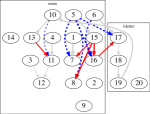
(a) oneword $-$ onechar

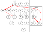
(b) oneline $-$ oneword

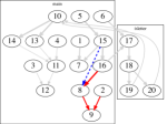
(c) multiline $-$ oneline

Figure 4. Differences in the CPDMs for word count created using the four different partitions of the test suite. In each figure A $-$ B, shows edges in A only in solid-red, edges in B only in dashed-blue, and edges in both in gray.

Differences in the Causal Program Dependence Models for word count created using the four different partitions of the test suite

4.1.1. Program Comprehension with Quantifiable Dependence

Filtering out edges based on their direct dependences reveals patterns that relate to features in the source code. Consider Figure 3(c) that only shows edges with strong direct dependence. Nodes connected in such edges often correspond to features that are executed in all executions. For example, nodes $\langle$5$\rangle$, $\langle$15$\rangle$, and $\langle$16$\rangle$, that are connected in Figure 3(c), collectively implement the function of reading a character from the input file. Similarly, nodes $\langle$1$\rangle$ and $\langle$7$\rangle$ increase the character count in each iteration. Nodes $\langle$2$\rangle$, $\langle$8$\rangle$, and $\langle$9$\rangle$ increase the line count, while $\langle$10$\rangle$, $\langle$13$\rangle$, and $\langle$14$\rangle$ determine if the current character is part of a word.

Figure 3(d) shows the edges with intermediate direct dependence values between 0.2 and 0.8. Compared to Figure 3(c), the connected nodes often reflect features that are only occasionally executed. For example, the word counting feature is only executed when there is at least one non-alphabet character in the input. Since seven out of 15 tests (three single character tests and four single word tests) do not have non-alphabet characters, the nodes implementing word counting feature consequently have small direct dependences for the whole test suite. Such dependences (denoted {from} $\rightarrow$ {to}) include {$\langle$20$\rangle$} $\rightarrow$ {$\langle$10$\rangle$} and {$\langle$14$\rangle$} $\rightarrow$ {$\langle$11$\rangle$}. Even a feature that is executed in every execution may have a small direct dependence. For example, the character read at node $\langle$16$\rangle$ affects the predicate at node $\langle$8$\rangle$, which in turn checks whether the character is a newline or not. Since among many characters, only newline character makes the difference, their causal relationship is not strong.

We posit that the capability to focus on different bands of direct dependences can help program comprehension. Despite being a small program of only about 40 lines, its PDG with equally weighted edges makes it difficult to understand the program semantics. To highlight the differences between PDG and CPDM, we discuss a few edges that are not found in the CPDM and why there are good, semantically meaningful reasons for this.

• {$\langle$5$\rangle$} $\rightarrow$ {all nodes control dependent on $\langle$5$\rangle$ except $\langle$15$\rangle$}: $\langle$5$\rangle$ and $\langle$15$\rangle$ are the predicates of the main loop. Therefore, all nodes within the loop are control dependent on the two. Since $\langle$15$\rangle$ is in the loop, if $\langle$5$\rangle$ changes, $\langle$15$\rangle$ also changes (along with all other nodes in the loop). In this case $\langle$5$\rangle$ is considered not as a direct parent of any of the other nodes in the loop and, consequently, CPDM produces the edge {$\langle$5$\rangle$} $\rightarrow$ {$\langle$15$\rangle$} while the PDG has many edges going out from $\langle$5$\rangle$.

• {$\langle$15$\rangle$} $\rightarrow$ {$\langle$8$\rangle$, $\langle$10$\rangle$, $\langle$17$\rangle$}: $\langle$8$\rangle$, $\langle$10$\rangle$, and $\langle$17$\rangle$ are control dependent on $\langle$15$\rangle$. However, they are also data dependent on $\langle$16$\rangle$, ($\langle$19$\rangle$, $\langle$20$\rangle$), or $\langle$16$\rangle$, respectively, which in turn depend on $\langle$15$\rangle$. If $\langle$15$\rangle$ changes, $\langle$16$\rangle$, $\langle$19$\rangle$, and $\langle$20$\rangle$ changes before $\langle$8$\rangle$, $\langle$10$\rangle$, and $\langle$17$\rangle$. Thus, the corresponding PDG edges are not in CPDM.

Let us now consider the relative strengths of dependence represented by the edge weights in CPDM. We highlight the following:

• {$\langle$19$\rangle$} $\rightarrow$ {$\langle$10$\rangle$} $>$ {$\langle$20$\rangle$} $\rightarrow$ {$\langle$10$\rangle$}: In function isLetter, $\langle$19$\rangle$ and $\langle$20$\rangle$ are the nodes that express whether the character is an alphabetic character or not. Since seven out of the 15 tests do not have a non-alphabet character, the effect on $\langle$10$\rangle$, which receives a return value of isLetter, of $\langle$19$\rangle$ is more significant than that of $\langle$20$\rangle$. It is important to keep in mind that the CPDM takes into account if a node’s behavior changes during execution, but not the number of different values it produces. Thus it is the number of tests cases and not their length that is important here.

• {$\langle$4$\rangle$} $\rightarrow$ {$\langle$11$\rangle$} $>$ {$\langle$13$\rangle$} $\rightarrow$ {$\langle$11$\rangle$} $>$ {$\langle$14$\rangle$} $\rightarrow$ {$\langle$11$\rangle$}: $\langle$4$\rangle$, $\langle$13$\rangle$, and $\langle$14$\rangle$ all correspond to the variable inword. $\langle$4$\rangle$ has the highest direct dependence on $\langle$11$\rangle$ because it affects whenever there exist more than zero alphabet characters. $\langle$13$\rangle$ and $\langle$14$\rangle$ affect $\langle$11$\rangle$ if the input includes more than one alphabet character. Because there are test cases that do not have any non-alphabet characters, $\langle$13$\rangle$ affects $\langle$11$\rangle$ more than $\langle$14$\rangle$.

4.1.2. Impact of Test Suites on CPDM

Let us consider the impact of building the CDPM for wc using the four categories of its test suites: onechar, oneword, oneline, and multiline. Figure 4(c) shows differences in the CPDMs constructed using different categories. The structure of CPDM changes according to the used category. In a figure labeled $A-B$, solid red edges are found only in $A$, dashed blue edges are found only in $B$, and gray edges are found in both $A$ and $B$. We highlight some of the findings below.

• One character versus multiple characters (Figure 4(a)): $\langle$15$\rangle$, $\langle$16$\rangle$, and $\langle$13$\rangle$ affect others only when there are more than one characters in the input. Therefore, there are outgoing edges from these in the CPDM of oneword but not in onechar. Instead, the direct predecessor nodes of $\langle$15$\rangle$, $\langle$16$\rangle$, and $\langle$13$\rangle$ ($\langle$5$\rangle$, $\langle$6$\rangle$, and $\langle$10$\rangle$) are linked to the nodes affected by $\langle$15$\rangle$, $\langle$16$\rangle$, and $\langle$13$\rangle$ in onechar.

• One word versus multiple words (Figure 4(b)): The sequence of edges {$\langle$18$\rangle$} $\rightarrow$ {$\langle$20$\rangle$} $\rightarrow$ {$\langle$10$\rangle$} $\rightarrow$ {$\langle$14$\rangle$} $\rightarrow$ {$\langle$11$\rangle$} is introduced in the CPDM created from oneline: the model reflects the information flow from reading a non-alphabet character to the increment of the word counter. Comparison with Figure 4(a) shows that the direct dependence of {$\langle$4$\rangle$} $\rightarrow$ {$\langle$11$\rangle$} and {$\langle$13$\rangle$} $\rightarrow$ {$\langle$11$\rangle$} have decreased due to the advent of a new node, $\langle$14$\rangle$, affecting $\langle$11$\rangle$. Note that, unlike in Figure 3(d), the direct dependence of {$\langle$19$\rangle$} $\rightarrow$ {$\langle$10$\rangle$} and {$\langle$20$\rangle$} $\rightarrow$ {$\langle$10$\rangle$} is similar. This is because every test in oneline contains both alphabet and non-alphabet characters.

• One line versus multiple lines (Figure 4(c)): With a newline character in the input, {$\langle$15$\rangle$} $\rightarrow$ {$\langle$8$\rangle$} disappears, while {$\langle$16$\rangle$} $\rightarrow$ {$\langle$8$\rangle$}, {$\langle$8$\rangle$} $\rightarrow$ {$\langle$9$\rangle$}, and {$\langle$2$\rangle$} $\rightarrow$ {$\langle$9$\rangle$} appear: the new edges represent counting of lines. Furthermore, using multiline makes the effect of $\langle$16$\rangle$ on $\langle$8$\rangle$ larger than that in Figure 3(d), because every test case contains a newline character.

Answer to RQ1: The numerical causality associated with each dependence tells us the strength of the causal connection between the two program elements involved. Our investigation shows that by exploiting these weights, CPDM can effectively focus a developer on dependencies of greater importance (those with higher causality). This focus provides a better understanding of the program.

Table 4. Acc@n for CDFL ($N_{mpn}=20$, median), SBFL, Dicing, and DS. Avg., LO, Max, and Min are different tiebreakers.

$n$	CDFL	SBFL				DS				Dicing
		Avg.	LO	Max	Min	Avg.	LO	Max	Min	Avg.	LO	Max	Min
1	8	3	10	3	21	0	0	0	92	3	7	3	9
3	19	11	14	9	26	0	3	0	92	7	7	7	9
5	27	17	18	12	41	0	6	0	92	7	7	7	9
10	43	31	40	27	59	2	12	0	92	7	8	7	9

4.2. Performance of CDFL

Here, we report the accuracy of CDFL in comparison to SBFL and other slice-based FL techniques.

4.2.1. Overall Performance of CDFL

Table 4 contains $acc@n$ metrics from the four studied FL techniques: CDFL, SBFL, Dynamic Slicing, and Dicing. The CDFL results are median values from ten trials, each based on CPDA computed with 20 sampled mutants (i.e., $N_{mpn}=20$). CDFL and SBFL outperform the slicing-based techniques for all values of $n$. CDFL performs better than SBFL rankings computed with the average tiebreaker: it can locate 166.6%, 72.7%, 58.8%, and 38.7% more faults in the top 1, 3, 5, and 10 places, respectively. Compared to SBFL with the line order tiebreaker, CDFL performs better in all cases except for $acc@1$. Note that SBFL, which is known to require diverse test cases for better performance (Steimann et al., 2013), suffers from the use of coverage adequate test suites that typically contain only one or two failing test cases. CDFL achieves better performance using the same test suite.

Since DS and Dicing use equally weighted dependence, all of their results are tied by definition. In most cases, the faulty line is executed by both passing and failing tests, which adversely affect the performance of dicing: among 92 faults, only nine faulty lines are found in the dice, all tied. SBFL is also vulnerable to ties, which can be seen from the results from minimum and maximum tie-breakers. On average, the number of tied program elements that are tied with the root cause is 20 for SBFL, and 95 for DS. In comparison, CDFL does not produce any ties.

4.2.2. Impact of Mutant Sampling on CDFL

To investigate the effect of the number of sampled mutants for each node, we vary the value of $N_{mpn}$ from 2 to 20 by intervals of two and repeat the CDFL analysis for each configuration. Our preliminary evaluation with $N_{mpn}\in\{30,40,50\}$ did not improve the accuracy of CDFL significantly beyond that obtained with $N_{mpn}=20$. Note that we increase $N_{mpn}$ by adding more samples (i.e., the set of samples with a larger $N_{mpn}$ includes the set with a smaller $N_{mpn}$): this is to avoid sampling bias when considering the effect of $N_{mpn}$.

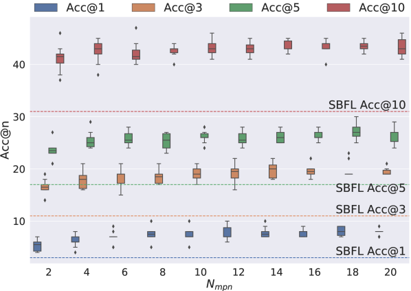
Figure 5. Acc@n of CDFL with different $N_{mpn}$ and SBFL using the average tiebreaker

Accuracy at n of Causal Dependence Fault Localization with different number of mutation samples per node and Spectra based Fault Localization using the average tiebreaker

Figure 5 shows boxplots of CDFL results from ten trials, obtained with varying $N_{mpn}$, in comparison to the results of SBFL, which are shown by the dashed horizontal lines. The boxplots initially show an increasing trend as $N_{mpn}$ increases. However, the trend tends to stabilize after $N_{mpn}=10$: the difference between median of $acc@n$ at $N_{mpn}=10$ and $N_{mpn}=20$ is less than, or equal to, one. The result suggests that, for the studied programs, ten mutation samples for each node is sufficient for fault localization.

Table 5. Acc@n for CDFL ($N_{mpn}=20$, median) and SBFL (avg. tie breaker) for each subject program

Program (# bugs)		tcas (34)				schedule (4)				schedule2 (3)				totinfo (18)				printtokens (3)				printtokens2 (6)				replace (24)
$n$		1	3	5	10	1	3	5	10	1	3	5	10	1	3	5	10	1	3	5	10	1	3	5	10	1	3	5	10
Acc@n	CDFL	4	10	14	23	0	1	1	2	1	1	1	1	0	1	2.5	3	0	1	1	2	1	2	2	3	2	3	4.5	9
	SBFL	0	3	7	10	0	0	1	1	0	0	0	0	0	0	0	3	0	0	1	1	1	2	2	3	2	6	6	13

4.2.3. Impact of Causal Structure on CDFL

Let us consider the impact that causal structure discovery has on the accuracy of CDFL. Table 5 presents the per-subject breakdown of $acc@n$ results from CDFL and SBFL. CDFL produces significantly higher $acc@n$ for tcas, while performing much worse than SBFL for replace. For other subjects, both techniques perform similarly well.

We posit that CDFL performs better for tcas due to its simpler control-flow structure. tcas is an aircraft collision avoidance system that calculates the altitude separation (Hutchins et al., 1994). The whole program is a sequence of logical formulas for the calculation of a single value, which requires minimal branching. Consequently, many computation steps are performed by both passing and failing test executions, presenting a challenge for SBFL. In comparison, CDFL considers both control and data dependency from the node trajectories, resulting in better performance.

In contrast, for many of the replace faults for which CDFL performs poorly, we find that the causal structure discovery is inadequate. By definition, a causal structure is a DAG, and cannot properly represent the cyclic dependence in a program. Breaking these cycles can lead to an incorrect set of Markovian parents, which in turn results in incorrect causal dependences. replace takes a a regex pattern, a substitution string, and a target text: it matches the pattern in the target text and replaces the match with the substitution string. During its operation, replace constructs lots of cyclic dependence relations between program elements. Such a large number of the cyclic dependencies cause CPDA to struggle to model the causal dependence accurately.

Answer to RQ2: CDFL can significantly outperform other slicing based fault localisation techniques. With sufficient mutant sampling, it can outperform SBFL and does not suffer from ties.

5. Discussion & Future Work

We currently use the definition of Markov parents directly in our algorithm to calculate causal dependences and the strengths of the causal connections in the CPDM. This is motivated by the fact that methods for causal discovery typically focus on observational data only, while we intervene in the program execution and thus have interventional data. Furthermore, our algorithm starts from binarized, indicator variables rather than from the raw observations. This is natural when, at least on the level of a high-level programming language, variables can contain complex structures such as trees.

However, in recent years there has been advances in learning causal structure also from interventional data and there are even algorithms for calculating optimal models with cycles (Rantanen et al., 2020). Future work should investigate how to apply these advances and tools in our setting. One challenge will be to bridge the gap from a high-level program with complex values in the nodes to methods that assume numerical data only. On the other hand, there might be several benefits, such as being able to handle cyclic dependences, as well as faster, more scalable structure learning (Ramsey et al., 2017).

6. Threats to Validity

Using a limited set of program inputs and approximating the dependence is a typical internal threat to any dynamic analysis, and thus also to CPDA. CPDA gets less effect from a small number of inputs through various mutations compared to dynamic slicing. RQ1 analyzes the effect of input by observing changes in CPDM when using different tests. For RQ2, we selected the tests based on the statement coverage criteria and used the same tests for other FL techniques to mitigate the threat. The sampling of mutants for CPDA poses another threat to the internal validity. To mitigate it, we sample a sufficiently large number of 100 mutants for RQ1, and conduct 10 independent trials for RQ2.

The use of the Siemens suite poses a threat to external validity. While we cannot claim that the result of RQ2 generalize, the Siemens suite is widely used in fault localization studies and enable comparison. We rely on a qualitative analysis for RQ1, and a widely studied metric ($acc@n$) for RQ2, to minimize the threat.

7. Related Work

This paper discusses two mainstream software engineering tasks: program dependence analysis and fault localization.

7.1. Program Dependence Analysis

Static analysis attempts to uncover facts about a program that apply to any possible execution. It is therefore necessarily conservative and consequently often produces many false positives. Static dependence analysis is often used to produce a Program Dependence Graph (PDG), which was first use in compiler optimization and parallelization (Ferrante et al., 1987), and has subsequently found many uses (Horwitz and Reps, 1992) including program slicing (Horwitz and Reps, 1992; Horwitz et al., 1990).

Dynamic dependence analysis incorporates one of more program inputs. A simple example is early dynamic slicing algorithms that computed a static slice of the PDG and then remove edges that are not executed (Agrawal and Horgan, 1990). Probabilistic Program Dependence Graph (PPDG) augments the PDG with a set of abstract states at each node that enable the use of probabilistic reasoning to analyze program behavior (Baah et al., 2010). Later, the Bayesian Network based Program Dependence Graph (BNPDG) augments the PDG with conditional probabilities to relate the state of a node to that of its parents (Yu et al., 2017).

In comparison, CPDM is not tied to PDG, freeing us from having to solve hard data-flow problems, such as pointer analysis. Instead, we extract the dependence structure from observations of program executions. We expect to further exploit the advances in the fields of causal inference and causal discovery to refine our approach. In contrast, PPDG (Baah et al., 2010) and BNPDG (Yu et al., 2017) are tied to the lower levels of the causal hierarchy as introduced by Pearl (Pearl, 2019) as they are based on the associative conditional probability between program states.

7.2. Fault Localization

Fault Localization (FL) aims to identify parts of the program source code that are likely to be the root cause of the observed test failures: typically FL techniques rank program elements by their relative likelihood of being the root cause (Wong et al., 2016). One of the most widely studied FL techniques is Spectrum Based Fault Localization (SBFL), a dynamic approach that ranks program elements based on their suspiciousness, which is computed from test coverage and outcomes (Steimann et al., 2013). SBFL has been widely studied both as an independent technique (Abreu et al., 2007; Xie et al., 2013; Naish et al., 2011) and in a hybridization with other FL input features and techniques (Sohn and Yoo, 2017; B. Le et al., 2016; Li et al., 2019; Le et al., 2015). However, it tends to produce many ties, as some program elements can share the same test coverage and outcome. Being based on coverage, SBFL also suffers from Coincidental Correctness (CC), i.e., passing executions that cover faulty elements (Masri and Assi, 2010).

Several existing work utilize the causal inference to fault localization. Baah et al. (Baah et al., 2010, 2011) use a linear model to capture the causal effect from coverage of program elements to test outcomes. Gore et al. (Gore and Reynolds, 2012) and Shu et al. (Shu et al., 2013) apply a similar linear regression approach to predicate values and method level coverage, respectively. In comparison, CDFL focuses on general dependence relations from CPDA instead of coverage, and therefore is less affected by CC.

8. Conclusion

We propose CPDA that measures strengths of dependence between program elements by modeling their causal relationship. Applying causal inference on observational data, instead of using static analysis, frees dependence analysis from the burden of pointer analysis and avoids producing large number of equally weighted dependence relations. Our evaluation of CPDM, a graph representation of a program causal relations, shows that CPDA can cluster semantically related program elements, based on meaningful differences in the strengths of program dependence. We also show the utility of continuously quantifiable program dependence by using it to create a novel fault localization method (CDFL). Our empirical evaluation shows that CDFL can outperform other FL techniques even with limited test suites. Future work will consider more advanced causal modeling with an emphasis on cyclic structures, as well as other applications of CPDA.

Appendix A Direct effect in CPDA

In this section, we reduce the formula of Definition 2.10.

Theorem A.1.

For a subset $X$ of random nodes,

$$P(s_{1},\cdots,s_{n}\mid\hat{x})=\begin{cases}\prod_{i\mid S_{i}\notin X}P(s_{i}\mid pa_{i})&\parbox{151.76964pt}{for $s_{1},\cdots,s_{n}$ consistent with $x$}\\ 0&\text{otherwise}\end{cases}\,.$$

Theorem A.2.

Let $G=(V,E)$ is a causal structure. Given two disjoint sets of nodes, $X,Y\in V$,

(1) $$P(y\mid\hat{x})=\sum_{\left(s_{i_{1}},\cdots,s_{i_{m}}\right)\mid S_{i}\notin Y}P(s_{1},\cdots,s_{n}\mid\hat{x})\,.$$

Corollary A.3.

$$P(y\mid\hat{x}^{\prime}) =\sum_{\left(s_{i_{1}},\cdots,s_{i_{m}}\right)\mid S_{i}\notin Y}P(s_{1},\cdots,s_{n}\mid\hat{x}^{\prime})$$

$$=\sum_{\left(s_{p_{1}},\cdots,s_{p_{q}}\right)\mid S_{p}\notin Y\cup X}\left[\sum_{\left(s_{r_{1}},\cdots,s_{r_{s}}\right)\mid S_{r}\notin Y\cup X^{c}}P(s_{1},\cdots,s_{n}\mid\hat{x}^{\prime})\right]$$

$$=\sum_{\left(s_{p_{1}},\cdots,s_{p_{q}}\right)\mid S_{p}\notin Y\cup X}\left[\sum_{s_{r_{1}}}\cdots\sum_{s_{r_{s-1}}}\sum_{s_{r_{s}}}P(s_{1},\cdots,s_{n}\mid\hat{x}^{\prime})\right]\,,$$

where $$\left\{s_{r_{1}},\cdots,s_{r_{s}}\right\}\in X\cap Y^{c}$$; since Theorem A.1,

$$=\sum_{\left(s_{p_{1}},\cdots,s_{p_{q}}\right)\mid S_{p}\notin Y\cup X}\left[\sum_{s_{r_{1}}}\cdots\sum_{s_{r_{s-1}}}P(s_{1},\cdots,s_{r_{s}}^{\prime},\cdots,s_{n}\mid\hat{x}^{\prime})\right]$$

$$=\cdots =\sum_{\left(s_{p_{1}},\cdots,s_{p_{q}}\right)\mid S_{p}\notin Y\cup X}P(s_{1},\cdots,s_{n}\mid\hat{x}^{\prime})$$

Corollary A.4.

For a statement $Y\in V$, using Corollary A.3,

$$P(y\mid\hat{pa}_{Y}) =\sum_{\left(s_{p_{1}},\cdots,s_{p_{q}}\right)\mid S_{p}\notin\left\{Y\right\}\cup PA_{Y}}P(s_{1},\cdots,s_{n}\mid\hat{pa}_{Y})$$

$$=\sum_{\left(s_{p_{1}},\cdots,s_{p_{q}}\right)\mid S_{p}\notin\left\{Y\right\}\cup PA_{Y}}\left[\prod_{j\mid S_{j}\notin PA_{Y}}P(s_{j}\mid pa_{j})\right]\quad\text{(by Theorem~{}\ref{equ:CE_set})}$$

$$=P(y\mid pa_{Y})\sum_{\left(s_{p_{1}},\cdots,s_{p_{q}}\right)\mid S_{p}\notin\left\{Y\right\}\cup PA_{Y}}\left[\prod_{j\mid S_{j}\notin\left\{Y\right\}\cup PA_{Y}}P(s_{j}\mid pa_{j})\right]$$

$$=P(y\mid pa_{Y})\,,$$

since $\sum_{\left(s_{p_{1}},\cdots,s_{p_{q}}\right)\mid S_{p}\notin\left\{Y\right\}\cup PA_{Y}}\left[\prod_{j\mid S_{j}\notin\left\{Y\right\}\cup PA_{Y}}P(s_{j}\mid pa_{j})\right]=1$.

Corollary A.5.

$$\mathit{DD}(S_{i},S_{j})$$

$$=\frac{1}{|I|}\sum_{i\in I}\mathit{NDE}_{O_{i},S_{i}:0\rightarrow 1}(S_{j})$$

$$=\frac{1}{|I|}\sum_{i\in I}\sum_{z}\left[\left\{E_{O_{i}}\left(S_{j}\mid do(S_{i}=1,z)\right)-E_{O_{i}}\left(S_{j}\mid do(S_{i}=0,z)\right)\right\}\right.$$

$$\qquad\qquad\qquad\left.\times\ P_{O_{i}}\left(z\mid do(S_{i}=0)\right)\right]$$

$$=\frac{1}{|I|}\sum_{i\in I}\sum_{z}\left[\left\{P_{O_{i}}\left(S_{j}=1\mid do(S_{i}=1,z)\right)-P_{O_{i}}\left(S_{j}=1\mid do(S_{i}=0,z)\right)\right\}\right.$$

$$\qquad\qquad\qquad\left.\times\ P_{O_{i}}\left(z\mid do(S_{i}=0)\right)\right]\,,$$

where $$Z=PA_{j}\backslash S_{i} \left\{S_{i}\right\}\cup Z=PA_{j}$$. Since , by Corollary A.4,

$$=\frac{1}{|I|}\sum_{i\in I}\sum_{z}\left[\left\{P_{O_{i}}\left(S_{j}=1\mid S_{i}=1,z\right)-P_{O_{i}}\left(S_{j}=1\mid S_{i}=0,z\right)\right\}\right.$$

$$\qquad\qquad\qquad\left.\times\ P_{O_{i}}\left(z\mid do(S_{i}=0)\right)\right]\,.$$

Here, by Corollary 2.7,

$$P_{O_{i}}(z\mid do(S_{i}=0))=\sum_{pa_{i}}P_{O_{i}}(z\mid S_{i}=0,pa_{i})P_{O_{i}}(pa_{i}).$$

References

- (1)
- Abreu et al. (2007) R. Abreu, P. Zoeteweij, and A. J. C. van Gemund. 2007. On the Accuracy of Spectrum-based Fault Localization. In Testing: Academic and Industrial Conference Practice and Research Techniques - MUTATION (TAICPART-MUTATION 2007). 89–98. https://doi.org/10.1109/TAIC.PART.2007.13
- Agrawal and Horgan (1990) Hiralal Agrawal and Joseph R. Horgan. 1990. Dynamic Program Slicing. SIGPLAN Not. 25, 6 (June 1990), 246–256. https://doi.org/10.1145/93548.93576
- Agrawal et al. (1995) H. Agrawal, J. R. Horgan, S. London, and W. E. Wong. 1995. Fault localization using execution slices and dataflow tests. In Proceedings of Sixth International Symposium on Software Reliability Engineering. ISSRE’95. 143–151. https://doi.org/10.1109/ISSRE.1995.497652
- B. Le et al. (2016) Tien-Duy B. Le, David Lo, Claire Le Goues, and Lars Grunske. 2016. A Learning-to-rank Based Fault Localization Approach Using Likely Invariants. In Proceedings of the 25th International Symposium on Software Testing and Analysis (ISSTA 2016). ACM, New York, NY, USA, 177–188.
- Baah et al. (2010) George K. Baah, Andy Podgurski, and Mary Jean Harrold. 2010. Causal inference for statistical fault localization. In Proceedings of the 19th International Symposium on Software Testing and Analysis (ISSTA 2010). ACM Press, 73–84.
- Baah et al. (2010) G. K. Baah, A. Podgurski, and M. J. Harrold. 2010. The Probabilistic Program Dependence Graph and Its Application to Fault Diagnosis. IEEE Transactions on Software Engineering 36, 4 (July 2010), 528–545. https://doi.org/10.1109/TSE.2009.87
- Baah et al. (2011) George K. Baah, Andy Podgurski, and Mary Jean Harrold. 2011. Matching Test Cases for Effective Fault Localization. Technical Report. Georgia Institute of Technology.
- Binkley (1997) D. Binkley. 1997. Semantics guided regression test cost reduction. IEEE Transactions on Software Engineering 23, 8 (Aug 1997), 498–516. https://doi.org/10.1109/32.624306
- Caillet et al. (2015) Pascal Caillet, Sarah Klemm, Michel Ducher, Alexandre Aussem, and Anne-Marie Schott. 2015. Hip fracture in the elderly: a re-analysis of the EPIDOS study with causal Bayesian networks. PLoS One 10, 3 (2015), e0120125.
- Collard et al. (2013) Michael Collard, Michael Decker, and Jonathan Maletic. 2013. srcML: An Infrastructure for the Exploration, Analysis, and Manipulation of Source Code: A Tool Demonstration. IEEE International Conference on Software Maintenance, ICSM, 516–519. https://doi.org/10.1109/ICSM.2013.85
- Do et al. (2005) Hyunsook Do, Sebastian Elbaum, and Gregg Rothermel. 2005. Supporting Controlled Experimentation with Testing Techniques: An Infrastructure and Its Potential Impact. Empirical Softw. Engg. 10, 4 (Oct. 2005), 405–435. https://doi.org/10.1007/s10664-005-3861-2
- Ettinger and Verbaere (2004) Ran Ettinger and Mathieu Verbaere. 2004. Untangling: a slice extraction refactoring. 93–101. https://doi.org/10.1145/976270.976283
- Feldt and Poulding (2013) Robert Feldt and Simon Poulding. 2013. Finding test data with specific properties via metaheuristic search. In 2013 IEEE 24th International Symposium on Software Reliability Engineering (ISSRE). IEEE, 350–359.
- Ferrante et al. (1987) Jeanne Ferrante, Karl J. Ottenstein, and Joe D. Warren. 1987. The Program Dependence Graph and its use in Optimization. 9, 3 (July 1987), 319–349.
- Gallagher and Lyle (1991) K. B. Gallagher and J. R. Lyle. 1991. Using program slicing in software maintenance. IEEE Transactions on Software Engineering 17, 8 (Aug 1991), 751–761. https://doi.org/10.1109/32.83912
- Gore and Reynolds (2012) Ross Gore and Paul F. Reynolds, Jr. 2012. Reducing Confounding Bias in Predicate-Level Statistical Debugging Metrics. In Proceedings of the 34th International Conference on Software Engineering (ICSE ’12). IEEE Press, 463–473.
- Grammatech Inc. (2002) Grammatech Inc. 2002. The CodeSurfer Slicing System. www.grammatech.com
- Horwitz and Reps (1992) Susan Horwitz and Thomas Reps. 1992. The Use of Program Dependence Graphs in Software Engineering. In International Conference on Software Engineering. Melbourne, Australia, 392–411.
- Horwitz et al. (1990) Susan Horwitz, Thomas Reps, and David Wendell Binkley. 1990. Interprocedural slicing using dependence graphs. 12, 1 (1990), 26–61.
- Hutchins et al. (1994) M. Hutchins, H. Foster, T. Goradia, and T. Ostrand. 1994. Experiments on the effectiveness of dataflow- and control-flow-based test adequacy criteria. In Proceedings of 16th International Conference on Software Engineering. 191–200. https://doi.org/10.1109/ICSE.1994.296778
- Jiang et al. (2017) Siyuan Jiang, Collin McMillan, and Raul Santelices. 2017. Do Programmers do Change Impact Analysis in Debugging? Empirical Software Engineering 22, 2 (01 Apr 2017), 631–669. https://doi.org/10.1007/s10664-016-9441-9
- Karim et al. (2018) R. Karim, F. Tip, A. Sochurkova, and K. Sen. 2018. Platform-Independent Dynamic Taint Analysis for JavaScript. IEEE Transactions on Software Engineering (2018), 1–1. https://doi.org/10.1109/TSE.2018.2878020
- Kirchner et al. (2015) Florent Kirchner, Nikolai Kosmatov, Virgile Prevosto, Julien Signoles, and Boris Yakobowski. 2015. Frama-C: A software analysis perspective. Formal Aspects of Computing 27, 3 (2015), 573–609. https://doi.org/10.1007/s00165-014-0326-7
- Le et al. (2015) Tien-Duy B. Le, Richard J. Oentaryo, and David Lo. 2015. Information Retrieval and Spectrum Based Bug Localization: Better Together. In Proceedings of the 2015 10th Joint Meeting on Foundations of Software Engineering (ESEC/FSE 2015). ACM, New York, NY, USA, 579–590. https://doi.org/10.1145/2786805.2786880
- Lee (2020) Seongmin Lee. 2020. Scalable and Approximate Program Dependence Analysis. In Proceedings of the ACM/IEEE 42nd International Conference on Software Engineering: Companion Proceedings (ICSE ’20). Association for Computing Machinery, New York, NY, USA, 162–165. https://doi.org/10.1145/3377812.3381392
- Lee et al. (2019) S. Lee, D. Binkley, R. Feldt, N. Gold, and S. Yoo. 2019. MOAD: Modeling Observation-Based Approximate Dependency. In 2019 19th International Working Conference on Source Code Analysis and Manipulation (SCAM). 12–22. https://doi.org/10.1109/SCAM.2019.00011
- Li et al. (2019) Xia Li, Wei Li, Yuqun Zhang, and Lingming Zhang. 2019. DeepFL: Integrating Multiple Fault Diagnosis Dimensions for Deep Fault Localization. In Proceedings of the 28th ACM SIGSOFT International Symposium on Software Testing and Analysis (ISSTA 2019). Association for Computing Machinery, New York, NY, USA, 169–180.
- Masri and Assi (2010) W. Masri and R.A. Assi. 2010. Cleansing Test Suites from Coincidental Correctness to Enhance Fault-Localization. In Software Testing, Verification and Validation (ICST), 2010 Third International Conference on. 165–174.
- Naish et al. (2011) Lee Naish, Hua Jie Lee, and Kotagiri Ramamohanarao. 2011. A model for spectra-based software diagnosis. ACM Transactions on Software Engineering Methodology 20, 3 (August 2011), 11:1–11:32.
- Ochiai (1957) A Ochiai. 1957. Zoogeographic studies on the soleoid fishes found in Japan and its neighbouring regions. Bulletin of the Japanese Society of Scientific Fisheries 22, 9 (1957), 526–530.
- Pearl (2009) Judea Pearl. 2009. Causality. Cambridge University Press. https://doi.org/10.1017/CBO9780511803161
- Pearl (2019) Judea Pearl. 2019. The seven tools of causal inference, with reflections on machine learning. Commun. ACM 62, 3 (2019), 54–60.
- Pearl et al. (2009) Judea Pearl et al. 2009. Causal inference in statistics: An overview. Statistics surveys 3 (2009), 96–146.
- Ramsey et al. (2017) Joseph Ramsey, Madelyn Glymour, Ruben Sanchez-Romero, and Clark Glymour. 2017. A million variables and more: the Fast Greedy Equivalence Search algorithm for learning high-dimensional graphical causal models, with an application to functional magnetic resonance images. International journal of data science and analytics 3, 2 (2017), 121–129.
- Rantanen et al. (2020) Kari Rantanen, Antti Hyttinen, and Matti Järvisalo. 2020. Learning Optimal Cyclic Causal Graphs from Interventional Data. In Proceedings of the 10th International Conference on Probabilistic Graphical Models (PGM 2020). Journal of Machine Learning Research.
- Richens et al. (2020) Jonathan G Richens, Ciarán M Lee, and Saurabh Johri. 2020. Improving the accuracy of medical diagnosis with causal machine learning. Nature communications 11, 1 (2020), 1–9.
- Shu et al. (2013) G. Shu, B. Sun, A. Podgurski, and F. Cao. 2013. MFL: Method-Level Fault Localization with Causal Inference. In 2013 IEEE Sixth International Conference on Software Testing, Verification and Validation. 124–133. https://doi.org/10.1109/ICST.2013.31
- Sohn and Yoo (2017) Jeongju Sohn and Shin Yoo. 2017. FLUCCS: using code and change metrics to improve fault localization. 273–283. https://doi.org/10.1145/3092703.3092717
- Spirtes and Zhang (2016) Peter Spirtes and Kun Zhang. 2016. Causal discovery and inference: concepts and recent methodological advances. In Applied informatics, Vol. 3. SpringerOpen, 1–28.
- Steimann et al. (2013) Friedrich Steimann, Marcus Frenkel, and Rui Abreu. 2013. Threats to the validity and value of empirical assessments of the accuracy of coverage-based fault locators. In Proceedings of the 2013 International Symposium on Software Testing and Analysis (ISSTA 2013). ACM, New York, NY, USA, 314–324.
- Untch et al. (1993) Roland H. Untch, A. Jefferson Offutt, and Mary Jean Harrold. 1993. Mutation Analysis Using Mutant Schemata. SIGSOFT Softw. Eng. Notes 18, 3 (July 1993), 139–148. https://doi.org/10.1145/174146.154265
- Wong et al. (2016) W. E. Wong, R. Gao, Y. Li, R. Abreu, and F. Wotawa. 2016. A Survey on Software Fault Localization. IEEE Transactions on Software Engineering 42, 8 (Aug 2016), 707–740. https://doi.org/10.1109/TSE.2016.2521368
- Xie et al. (2013) Xiaoyuan Xie, Tsong Yueh Chen, Fei-Ching Kuo, and Baowen Xu. 2013. A Theoretical Analysis of the Risk Evaluation Formulas for Spectrum-based Fault Localization. ACM Transactions on Software Engineering Methodology 22, 4 (October 2013), 31:1–31:40.
- Yu et al. (2017) Xiao Yu, Jin Liu, Zijiang Yang, and Xiao Liu. 2017. The Bayesian Network based program dependence graph and its application to fault localization. Journal of Systems and Software 134 (2017), 44 – 53. https://doi.org/10.1016/j.jss.2017.08.025
- Zhifeng Yu and Rajlich (2001) Zhifeng Yu and V. Rajlich. 2001. Hidden dependencies in program comprehension and change propagation. In Proceedings 9th International Workshop on Program Comprehension. IWPC 2001. 293–299. https://doi.org/10.1109/WPC.2001.921739