Dynamics of equilibration and collisions in ultradilute quantum droplets

Abstract

Employing time-dependent density-functional theory, we have studied dynamical equilibration and binary head-on collisions of quantum droplets made of a ³⁹K-³⁹K Bose mixture. The phase space of collision outcomes is extensively explored by performing fully three-dimensional calculations with effective single-component QMC based and two-components LHY-corrected mean-field functionals. We exhaustively explored the important effect –not considered in previous studies– of the initial population ratio deviating from the optimal mean-field value $N_{2}/N_{1}=\sqrt{a_{11}/a_{22}}$. Both stationary and dynamical calculations with an initial non-optimal concentration ratio display good agreement with experiments. Calculations including three-body losses acting only on the $\ket{F,m_{F}}=\ket{1,0}$ state show dramatic differences with those obtained with the three-body term acting on the total density.

I Introduction

The collision of liquid drops is one of the more fundamental and complex problems addressed in fluid dynamics, with implications in basic research and applications e.g. in microfluidics, formation of rain drops, ink-jet printing, or spraying for combustion, painting and coating Ashgriz and Poo (1990); Qian and Law (1997); Pan et al. (2009); Varma et al. (2016). Liquid drop collisions were also used as a model for nucleus-nucleus reactions Swiatecki (1982) and nanoscopic ³He droplets collisions Guilleumas et al. (1995).

Generally speaking, upon collision droplets may bounce back, coalesce into a single drop, separate after temporarily forming a partially fused system, or shatter into a cloud of small droplets. The main goal of the studies on droplet-droplet collisions is to determine how the appearance of these regimes depends on the collision parameters (droplet size, velocity, impact parameter) and intrinsic properties of the liquid (viscosity, surface tension, …).

With the advent of the so-called “helium drop machines”, it has been possible to generate ⁴He nanodroplets by the free expansion of a supercooled gas, as reviewed e.g. in Ref. Toennies and Vilesov (2004). This has allowed to extend the study of liquid droplets to the quantum regime. Indeed, helium in its two isotopic forms, ³He (a fermion) and ⁴He (a boson), is the only element in nature which may exist at zero temperature as an extended liquid or in the form of droplets. Superfluid ⁴He samples are ideal systems to study quantized vortices –a most striking hallmark of superfluidity Donnelly (1993)– and quantum turbulence Tsubota and Halperin (2009).

At the experimental droplet temperatures, 0.37 K for ⁴He and 0.15 K for ³HeToennies and Vilesov (2004), ⁴He is a superfluid and ³He is a normal fluid. Studies on superfluid ⁴He droplets collisions are very scarce, see e.g. Refs. Vicente et al. (2000); Maris (2003); Ishiguro et al. (2004); Escartín et al. (2019). It has been recently shown that the merging of superfluid ⁴He nanodroplets may produce quantized vortices and surface turbulence Nazarenko (2015); Escartín et al. (2019)

In the field of ultracold Bose gases, there are also very few studies of cold gas collisions Sun and Pindzola (2008); Astrakharchik and Malomed (2018); Zhong (2021), since the only accessible phase until recently was the gaseous, confined one. Nevertheless, there are many interesting dynamical phenomena Pitaevskii and Stringari (2016) whose description has attracted interest, such as the study of collective excitations in confined Bose and Fermi systems, with different dimensionalities, in gaseous Dalfovo et al. (1999); Jin et al. (1996); Pollack et al. (2010); Skov et al. (2020); Atas et al. (2017); De Rosi and Stringari (2015); Kinast et al. (2004); Bartenstein et al. (2004); Altmeyer et al. (2007), liquid Tylutki et al. (2020); Hu and Liu (2020a) or supersolid regimes Tanzi et al. (2019); Léonard et al. (2017).

The situation has changed quite recently since a self-bound, low-density liquid-like state composed by ultracold quantum Bose-Bose mixtures, first theoretically proposed by Petrov Petrov (2015), has been experimentally produced Cabrera et al. (2018); Cheiney et al. (2018); Semeghini et al. (2018); D’Errico et al. (2019). In these mixtures, an adequately tuned interaction can lead to a regime where the mean-field energy is comparable to the Lee, Huang, and Yang (LHY) energy. The LHY energy term is a perturbative correction to the mean-field energy, first calculated with the single-component Bose gas Lee and Yang (1957); Huang and Yang (1957), and later extended to two-component Bose-Bose mixtures Larsen (1963); Minardi et al. (2019); Naidon and Petrov (2021). This desirable feature of stabilizing the mean-field collapse in an LHY-extended theory (MF+LHY), allowing for droplet formation, is present also in low-dimensional geometries Petrov and Astrakharchik (2016); Parisi et al. (2019); Parisi and Giorgini (2020) and accounts for the stability of dipolar droplets Böttcher et al. (2019, 2021). Consequently, the realm of stable quantum droplets has been extended to densities much lower than those of helium droplets Barranco et al. (2006).

As pointed out in Ref. Hu and Liu (2020b), the LHY term suffers from an intrinsic inconsistency with the appearance of an imaginary term in the energy of the Bose-Bose mixture. This is at variance with a single-component Bose gas, where no such imaginary term appears, and where the LHY term has proven to be valid up to relatively large densities, as it was confirmed by first-principle Quantum Monte Carlo (QMC) calculations Giorgini et al. (1999); Rossi and Salasnich (2013). Already in the first experimental realization of a quantum Bose-Bose liquid mixture, composed by two hyperfine states of ³⁹K, there have been deviations of observed properties from the predictions of usually employed theory based on interactions described solely in terms of $s$-wave scattering lengths Petrov (2015). These effects were properly explained instead by a QMC-based functional built to include effective-range corrections Cikojević et al. (2020). Diffusion Monte Carlo (DMC) calculations indicate that inclusion of the effective range allows to extend the universality of the theory Cikojević et al. (2019, 2020), providing improved energy functionals when both the $s$-wave scattering lengths and the effective ranges are known.

Some progress in the understanding of dynamical properties of quantum Bose-Bose droplets has been made in a recent experimental study of head-on collisions between pairs of ³⁹K-³⁹K droplets Ferioli et al. (2019), providing a new avenue of research. In Ref. Ferioli et al. (2019), the authors discovered a highly compressible droplet regime, not present in the world of classical liquids, when the total atom numbers in colliding droplets are small. Thus, it is not clear whether the Weber number theory Frohn and Roth (2000), describing the dynamics of classical liquid collisions, can apply to ultra-dilute droplets. Depending on the velocity of each droplet, the outcome of the experiment Ferioli et al. (2019) was either merging or separation of the colliding droplets.

As in Ref. Ferioli et al. (2019), we define a critical velocity $v_{c}$ as the initial velocity of each droplet above (below) which the two droplets separate (merge) upon colliding. A significant discrepancy was observed between the experimental critical velocity $v_{c}$ and the theoretical analysis of the experiment carried out within the MF+LHY approach Ferioli et al. (2019). The disagreement was attributed to the lacking of three-body losses (3BL), which were introduced in a next step but acting on the total density. This means that both components lose their atoms such that the density ratio is constantly kept fixed at the value $\rho_{2}/\rho_{1}=\sqrt{a_{11}/a_{22}}$, which is the mean-field stability requirement Petrov (2015); Staudinger et al. (2018); Ancilotto et al. (2018). By doing so, the agreement between theory and experiment was found to be good. However, it is unclear whether this procedure masks other interesting details which might be hidden by the fact that 3BL are made to act on the total density and not on the appropriate component of the bosonic mixture. In particular, the procedure excludes the possibility that the droplets in the experiment are not fully equilibrated. Additionally, experimental measures Semeghini et al. (2018) have demonstrated significant differences in intensities of 3BL of different components, which are not taken into account by the approach of Ref. Ferioli et al. (2019). In this work, we re-analyze that experiment by using a QMC-based functional which takes into account the effective range of the interactions and a two-component MF+LHY functional that enables the study of unequilibrated drops and an experimentally more realistic consideration of 3BL. Our results show the relevance of the non-optimal concentration ratio in the outcome of drop collisions, providing an alternative explanation to the experimental results without invoking 3BL.

This work is organized as follows. In Sec. II we lay out the basic equations of the extended LHY mean-field theory (MF+LHY). In Sec. III we present the details of our simulations. In Sec. IV we discuss the effects of the non-optimal initial atom number ratio and 3BL on the stationary drop. In Sec. V.1, we systematically compare the drops collisions results obtained within the effective single-component MF+LHY theory with those obtained using the QMC-based functional. In Sec. V.2 we report results derived with the two-component framework. In Sec. V.3 we investigate the influence on the collisions of both the initial population imbalance and 3BL acting only on the $\ket{F,m_{F}}=\ket{1,0}$ state. Finally, Sec. VI comprises the main conclusions of our work.

II MF+LHY and QMC density functionals

The LHY-extended mean-field theory (MF+LHY) is based on the following density functional per unit volume $V$ Petrov (2015); Ancilotto et al. (2018),

$$\mathcal{E}[\rho_{1},\rho_{2}]=E_{\rm MF}/V+E_{\rm LHY}/V\ ,$$ (1)

where

$$\dfrac{E_{\rm MF}}{V}=\dfrac{2\pi\hbar^{2}a_{11}}{m}\rho_{1}^{2}+\dfrac{2\pi\hbar^{2}a_{22}}{m}\rho_{2}^{2}+\dfrac{4\pi\hbar^{2}a_{12}}{m}\rho_{1}\rho_{2}\ ,$$ (2)

and

$$\dfrac{E_{\rm LHY}}{V}=\dfrac{256\sqrt{\pi}\hbar^{2}}{15m}(a_{11}\rho_{1})^{5/2}f\left(1,\dfrac{a_{12}^{2}}{a_{11}a_{22}},\dfrac{a_{22}\rho_{2}}{a_{11}\rho_{1}}\right)\ .$$ (3)

We have considered equal masses $m_{1}=m_{2}=m$ and the function $f$ is defined in Ref. Petrov (2015),

$$f(1,u,x)=\dfrac{1}{{4\sqrt{2}}}[(1+x+\sqrt{(1-x)^{2}+4ux})^{5/2}$$

$$+(1+x-\sqrt{(1-x)^{2}+4ux})^{5/2}]\ .$$ (4)

Here $u={a_{12}^{2}}/{(a_{11}a_{22})}$ and $x={a_{22}\rho_{2}}/{(a_{11}\rho_{1})}$. The function $f$ is complex for $a_{12}^{2}>a_{11}a_{22}$, and we use the approximation ${a_{12}^{2}}={a_{11}a_{22}}$ to keep $f$ real. By doing so, $f(1,1,x)=(1+x)^{5/2}$ and the LHY functional reads

$$\dfrac{E_{\rm LHY}}{V}=\dfrac{256\sqrt{\pi}\hbar^{2}}{15m}\left(a_{11}\rho_{1}+a_{22}\rho_{2}\right)^{5/2}.$$ (5)

The above framework is the most general version of a two-component equal-masses Bose-Bose energy functional, and it allows for all possible $\rho_{1}$ and $\rho_{2}$ values. This functional can be reduced to an effective one-component functional, which is the one mostly used in the study of Bose-Bose mixtures, if one uses the result that the stability of a dilute Bose-Bose mixture lies in a very narrow range of optimal partial densities $\rho_{1}/\rho_{2}=\sqrt{a_{22}/a_{11}}$ Staudinger et al. (2018); Ancilotto et al. (2018). Then, for this fixed ratio of $\rho_{1}/\rho_{2}$ the MF+LHY theory can be written in the compact form

$$\dfrac{E/N}{|E_{0}|/N}=-3\left(\dfrac{\rho}{\rho_{0}}\right)+2\left(\dfrac{\rho}{\rho_{0}}\right)^{3/2}\ ,$$ (6)

with $\rho$ being the total density and $E_{0}/N$ and $\rho_{0}$ the equilibrium energy per particle and equilibrium total density, respectively, given by

$$\rho_{0}=\dfrac{25\pi}{1024}\dfrac{\left(a_{12}/a_{11}+\sqrt{a_{22}/a_{11}}\right)^{2}}{\left(a_{22}/a_{11}\right)^{3/2}\left(1+\sqrt{a_{22}/a_{11}}\right)^{4}}\dfrac{1}{a_{11}^{3}}\ ,$$ (7)

$$\dfrac{E_{0}}{N}=\dfrac{-\hbar^{2}}{ma_{11}^{2}}\dfrac{25\pi^{2}}{768}\dfrac{|a_{12}/a_{11}+\sqrt{a_{22}/a_{11}}|^{3}}{a_{22}/a_{11}(1+\sqrt{a_{22}/a_{11}})^{6}}=\dfrac{-\hbar^{2}}{2m\xi^{2}}\ .$$ (8)

We have introduced in the last equation the healing length $\xi$, obtained by equating the kinetic energy to the energy per particle at the equilibrium density:

$$\dfrac{\xi}{a_{11}}=\dfrac{8\sqrt{6}}{5\pi}\sqrt{\dfrac{a_{22}}{a_{11}}}\dfrac{(1+\sqrt{a_{22}/a_{11}})^{3}}{|a_{12}/a_{11}+\sqrt{a_{22}/a_{11}}|^{3/2}}\ .$$ (9)

The total atom number in the reduced unit $\tilde{N}$ introduced in Ref. Petrov (2015), is given by

$$\dfrac{N}{\tilde{N}}=\dfrac{3\sqrt{6}}{5\pi^{2}}\dfrac{\left(1+\sqrt{a_{22}/a_{11}}\right)^{5}}{|a_{12}/a_{11}+\sqrt{a_{22}/a_{11}}|^{5/2}}\ .$$ (10)

To compare with the results of Ref. Ferioli et al. (2019), the velocity $v$ can be expressed in the universal unit $\tilde{v}$ as

$$\dfrac{v}{\tilde{v}}=\dfrac{5\pi\hbar}{8\sqrt{6}ma_{11}}\dfrac{|a_{12}/a_{11}+\sqrt{a_{22}/a_{11}}|^{3/2}}{\sqrt{a_{22}/a_{11}}(1+\sqrt{a_{22}/a_{11}})^{3}}\ .$$ (11)

We have also used a density functional derived from QMC calculations (QMC functional in the following), which is constructed by performing DMC calculations of a ³⁹K mixture in the homogeneous phase Cikojević et al. (2020). The QMC functional $\mathcal{E}_{\rm int}$ is obtained with the relation

$$\mathcal{E}_{\rm int}=\rho\dfrac{E}{N},$$ (12)

where $E/N$ is the energy per particle of the extended system, calculated from QMC. QMC calculations were performed with the model potentials which reproduce both the $s$-wave scattering lengths and effective ranges, which are known from the experiment Tanzi et al. (2018). In this way, the QMC functional correctly incorporates the two relevant scattering parameters of this mixture, i.e., the $s$-wave scattering lengths and the effective ranges.

III Time-evolution equations

For a two-component system, our ansatz for the many-body wave function is

$$\Psi(\mathbf{r}_{1},\ldots,\mathbf{r}_{N};t)=\prod_{i=1}^{N_{1}}\psi_{1}(\mathbf{r}_{i},t)\prod_{j=1}^{N_{2}}\psi_{2}(\mathbf{r}_{j},t),$$ (13)

where the number of particles of component 1 (2) is equal to $N_{1}$ ($N_{2}$). The equations of motion for the two components read

$$i\hbar\dfrac{\partial\psi_{i}}{\partial t}=\mathcal{H}_{i}\psi_{i}=\left\{-\dfrac{\hbar^{2}}{2m}\nabla^{2}+V_{i}(\rho_{1},\rho_{2})\right\}\psi_{i}\ ,$$ (14)

for $i=1,2$, where $\rho_{i}=|\psi_{i}|^{2}$, and the potential $V_{i}$ is obtained from Eq. (1) Barranco et al. (2017)

$$V_{i}=\dfrac{\partial\mathcal{E}[\rho_{1},\rho_{2}]}{\partial\rho_{i}}\ .$$ (15)

Explicitly, the coupled equations of motion for the two components of the condensate read

$$i\hbar\frac{\partial\psi_{1}}{\partial t} = \left(-\frac{\hbar^{2}}{2m}\nabla^{2}+\dfrac{4\pi\hbar^{2}a_{11}}{m}\rho_{1}\right.+\dfrac{4\pi\hbar^{2}a_{12}}{m}\rho_{2}+$$ (16)

$$\frac{128\sqrt{\pi}\hbar^{2}a_{11}}{3m}\left(a_{11}\rho_{1}+a_{22}\rho_{2}\right)^{3/2}\bigg{)}\psi_{1}\ ,$$

$$i\hbar\frac{\partial\psi_{2}}{\partial t} = \left(-\frac{\hbar^{2}}{2m}\nabla^{2}+\dfrac{4\pi\hbar^{2}a_{22}}{m}\rho_{2}\right.+\dfrac{4\pi\hbar^{2}a_{12}}{m}\rho_{1}+$$ (17)

$$\frac{128\sqrt{\pi}\hbar^{2}a_{22}}{3m}\left(a_{11}\rho_{1}+a_{22}\rho_{2}\right)^{3/2}\bigg{)}\psi_{2}\ .$$

When the ratio of densities is the optimal one, $\rho_{2}/\rho_{1}=\sqrt{a_{11}/a_{22}}$, fixed by the condition of minimum energy per particle Petrov (2015); Staudinger et al. (2018); Ancilotto et al. (2018), the energy functional for the total density $\rho=\rho_{1}+\rho_{2}$ reduces to

$$\mathcal{E}_{\rm int}=\alpha\rho^{2}+\beta\rho^{\gamma+1},$$ (18)

where $\alpha$, $\beta$ and $\gamma$ are either the MF+LHY parameters from Eq. (6), or the ones which better fit the DMC equation of state Cikojević et al. (2020). In this case, the problem is thus effectively single-component, meaning that the full many-body wavefunction (13) reduces to

$$\Psi(\mathbf{r}_{1},{\bm{r}}_{2},\ldots,\mathbf{r}_{N};t)=\prod_{i=1}^{N}\psi(\mathbf{r}_{i};t),$$ (19)

where $\psi$ is the solution of the following equation

$$i\hbar\dfrac{\partial\psi}{\partial t}=\mathcal{H}\psi=\left(\dfrac{-\hbar^{2}}{2m}\nabla^{2}+V(\rho)\right)\psi\ ,$$ (20)

where

$$V(\rho)=2\alpha\rho+\beta(\gamma+1)\rho^{\gamma}\ .$$ (21)

Equations (16), (17) and (20) are solved numerically by successively applying the time-evolution operator

$$\psi(t+\Delta t)=e^{-i\mathcal{H}\Delta t}\psi(t)\ ,$$ (22)

where a Trotter decomposition accurate to second order in the time step is implemented Chin et al. (2009)

$$e^{-i\mathcal{H}\Delta t/\hbar}=e^{-i\Delta tV(\mathbf{R}^{\prime})/2\hbar}e^{-i\Delta t\hat{K}/\hbar}e^{-i\hbar\Delta tV(\mathbf{R})/2\hbar}+\mathcal{O}(\Delta t^{3})\ ,$$ (23)

with $\hat{K}=-\hbar^{2}\nabla^{2}/(2m)$. The kinetic energy propagator is evaluated in $k$-space by means of Fourier transforms.

Since an important parameter in our study is the deviation with respect to the optimal atom ratio $N_{2}/N_{1}=\sqrt{a_{11}/a_{22}}$, we define the atom ratio $x$ as

$$x=\frac{N_{2}}{N_{1}}\sqrt{\frac{a_{22}}{a_{11}}}\ ,$$ (24)

such that $x=1$ corresponds to the optimal mean-field composition. Note that one only needs to address the case $x\leq 1$ due to the symmetric role of atom numbers.

IV Real-time relaxation of an isolated droplet

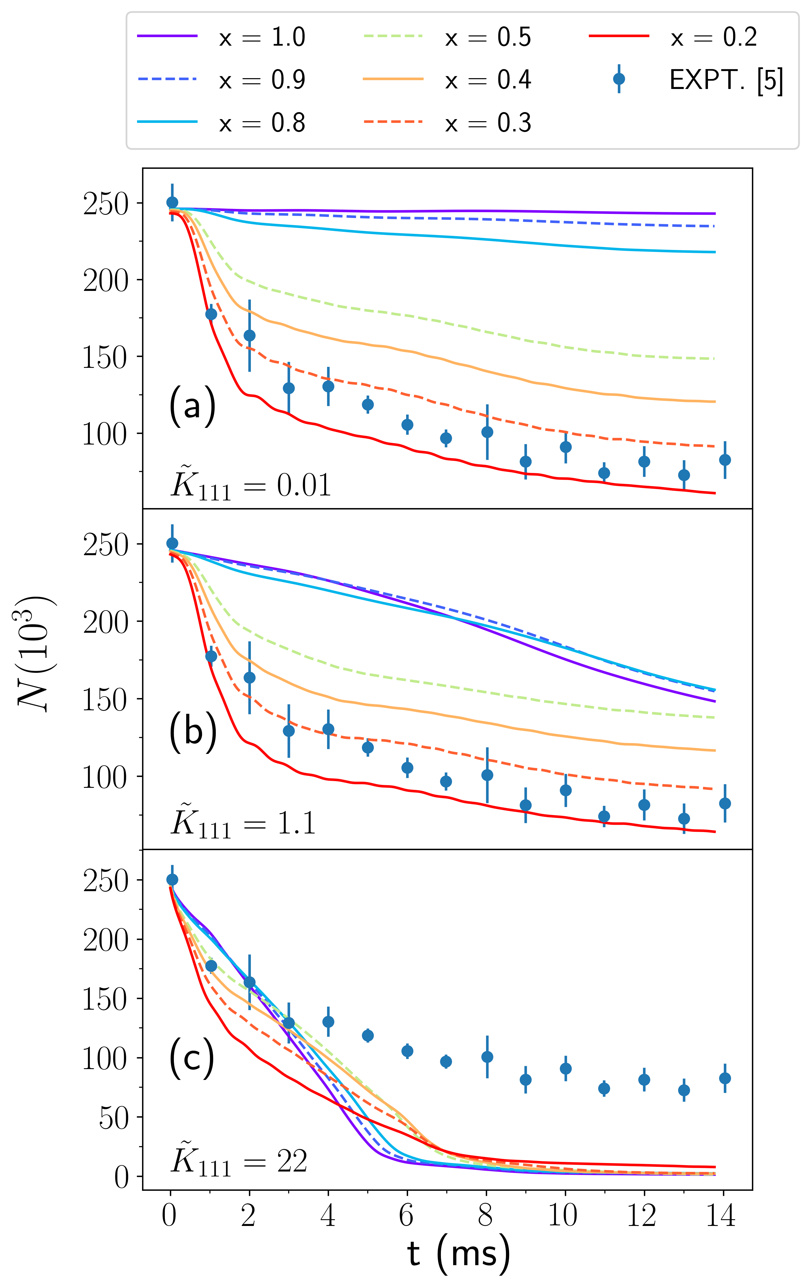
Figure 1: Time evolution of the total atom number $N$ in a stationary droplet. Lines are the results of two-component MF+LHY+3BL calculations, and points are experimental data from Ref. Semeghini et al. (2018). The initial atom number is $N=2.5\times 10^{5}$, with Gaussians of width $\sigma_{r}=3\mu$m as density profiles. The values of $x=(N_{2}/N_{1})\sqrt{a_{22}/a_{11}}$ imposed at $t=0$ are given in the top legend. The 3BL coefficients are shown in the panels in units of $\hbar/(m\xi^{2}\rho_{0}^{2})$, with $\rho_{0}$ and $\xi$ being the equilibrium density and healing length given in Table 1.

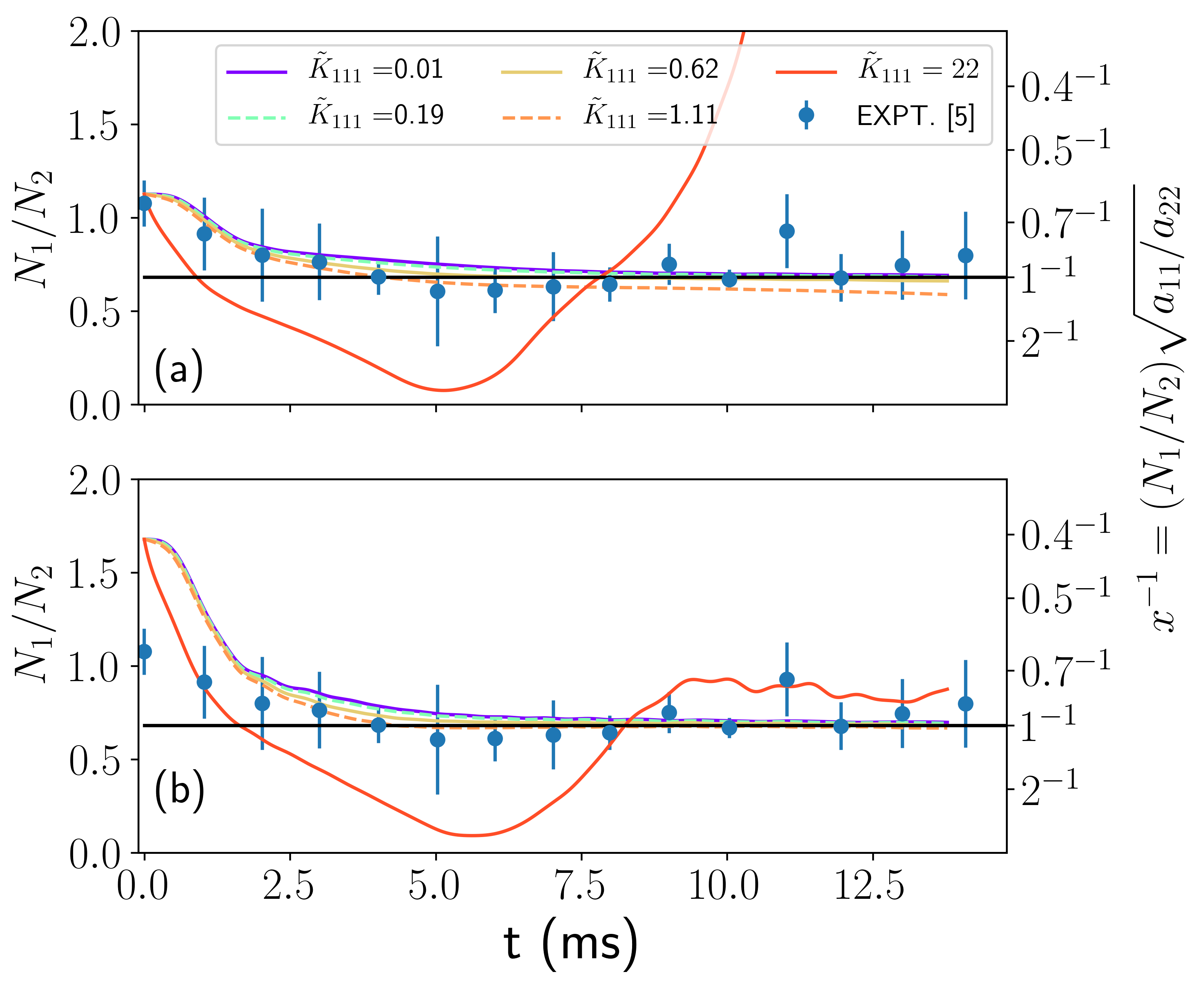
Figure 2: Time evolution of $N_{1}/N_{2}$ for the same simulations as in Fig. 1. Starting atom number imbalances: panel (a), $x=0.7$; panel (b): $x=0.4$. Points are data from the Ref. Semeghini et al. (2018).

We first focus our attention on the time evolution of a ³⁹K-³⁹K droplet as observed in the Florence experiment [Fig. (2) in Ref. Semeghini et al. (2018)]. We performed two-component MF+LHY calculations with the goal to investigate the influence of the initial non-optimal population ratio and 3BL on the real-time dynamics. To mimic the experimental setup, at $t=0$ we set the shape of a $N=2.5\times 10^{5}$ atoms droplet as a Gaussian of width $\sigma_{r}=3\,\mu$m and let the system evolve according to the extended Gross-Pitaevskii equations (16) and (17). The scattering parameters $a_{ij}$ correspond to the magnetic field $B=56.54$ G (see Table 1). We denote the $\ket{F,m_{F}}=\ket{1,0}$ state as component 1 and the $\ket{F,m_{F}}=\ket{1,-1}$ state as component 2. Within the two-component MF+LHY approach, we show in Fig. 1 the time evolution of the total atom number, inside a volume of a cube with $12\mu$m length centered in the origin of the simulation box, for different initial atom ratios ranging from $x=0.2$ to $x=1$. This was done changing the normalization of each component to the desired value at $t=0$, keeping fixed the total number of atoms, $N=2.5\times 10^{5}$. We have included 3BL only in the time evolution of the $\psi_{1}$ component, whose 3BL coefficient is reported to be at least 100 times larger than the 3BL coefficients in the other channels Semeghini et al. (2018); Ferioli et al. (2020). This effect is included by introducing a term $-i\hbar K_{111}|\psi_{1}|^{4}/2$ in Eq. (16). We have explored three different values of $K_{111}$, namely $0$, $1.1$ and 22 in units of $\hbar/(m\xi^{2}\rho_{0}^{2})$, which correspond to $0$, $5.5\times 10^{-28}\mathrm{~{}cm}^{6}/\mathrm{s}$ and $1.1\times 10^{-26}\mathrm{~{}cm}^{6}/\mathrm{s}$, respectively (see Table 1 for units).

Notice that there is a large experimental uncertainty affecting the actual value of $K_{111}$: both non-zero values we choose here are compatible with the experimental error bar in the determination of the 3BL term for the ³⁹K-³⁹K mixture. The largest of these $K_{111}$ values was used in the two-component calculations in Ref. Semeghini et al. (2018) to explain the time evolution of the drop size observed in the experiment Semeghini et al. (2018). Looking at Fig. 1, it is clear that this value of $K_{111}$ predicts too strong 3BL. For smaller $K_{111}$ values (panels (a) and (b) in Fig. 1), similar to those reported in Ref. Ferioli et al. (2019), we observe that compared to the atom number imbalance $x$, 3BL play a minor role in the equilibration process. The relative atom number obtained from our calculations is also consistent with the experimental data as shown in Fig. 2, where we display the evolution of relative atom number, starting from $x=0.7$ (panel a), and $x=0.4$ (panel b). The only exception is for the largest $K_{111}$ value which deviate significantly from the experimental results. The observed atom loss can thus be mainly attributed to the droplet equilibration process in which the excess component is expelled until the optimal atom number ratio is eventually reached. A much lesser contribution to the equilibration arises from 3BL.

Table 1: Scattering parameters, i.e. $s$-wave scattering lengths $a$, in units of Bohr radius $a_{0}$, as a function of the magnetic field $B$ Roy et al. (2013). $\xi$ and $\rho_{0}$ stand for healing length and equilibrium density of uniform liquid, respectively (see Eqs. 9 and 7).

$B({\rm G})$	$a_{11}(a_{0})$	$a_{22}(a_{0})$	$a_{12}(a_{0})$	$\xi(\mathrm{\mu m})$	$\rho_{0}(\mathrm{cm}^{-3})$
56.23	63.648	34.587	-53.435	0.496	$5.773\times 10^{15}$
56.54	72.960	33.962	-53.293	1.479	$1.217\times 10^{15}$
56.55	73.3	33.9	-53.3	1.527	$1.164\times 10^{15}$

V Droplets collisions

We study the phase diagram characterizing the outcome of head-on binary collisions using the same description as in Ref. Ferioli et al. (2019), i.e., in terms of $({v},{N}_{\rm coll})$, where ${N}_{\rm coll}={N}(t=t_{\rm coll})$ is the total atom number evaluated at the collision time $t_{\rm coll}$, and ${v}$ is velocity of each droplet at the beginning of the simulation. The collision time $t_{\rm coll}$ is estimated as $t_{\rm coll}=d/(2v)$, where $d$ is the initial distance between the two droplets. The initial wavefunction reads

$$\psi(t=0)=\phi(x-d/2,y,z)e^{+ikx}+\phi(x+d/2,y,z)e^{-ikx},$$ (25)

where $\phi$ and $k=mv/\hbar$ are the wave function and wave number of each droplet, respectively. Note that in all figures the total atom number $N$ and velocity $v$ are re-scaled according to Eqs. (10) and (11).

For all the simulations performed in this work we have observed three possible collision outcomes: (i) for small velocities, merging of the droplets into a single one (coalescence appears after substantial deformation of the droplets), (ii) for higher velocities, separation, where the two droplets move away from one another after the collision, and (iii) evaporation, which occurs for very energetic collisions. Shattering is not observed because BEC drops must have a minimum size to be bound Petrov (2015) and instead of a cloud of small droplets the process continues until complete evaporation.

This is illustrated in Fig. 3, where one may see the three outcomes: merging (Fig. 3a), separation (Fig. 3b), and evaporation (Fig. 3c). The simulation corresponds to the two-component calculations described below.

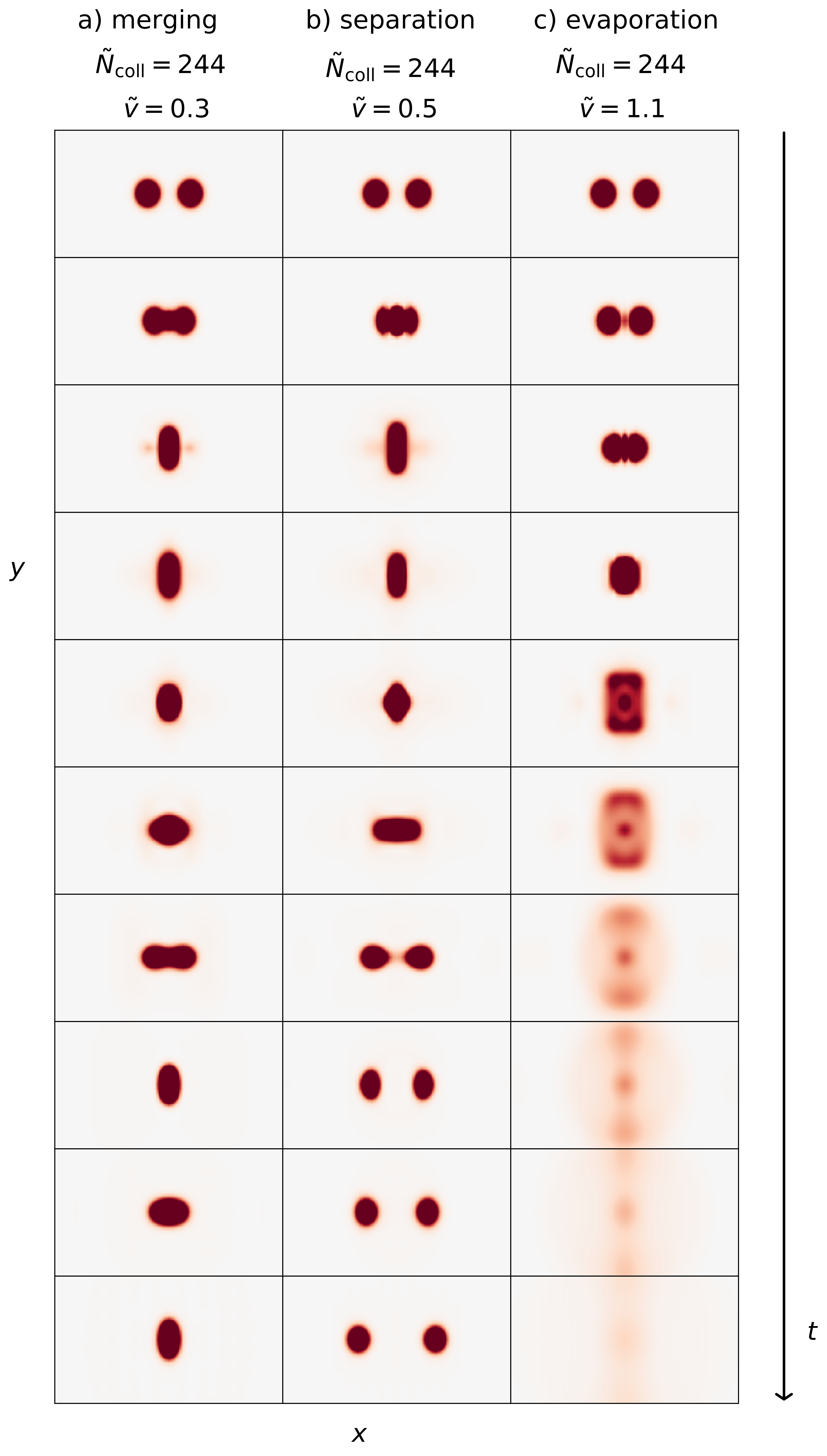
Figure 3: Three possible outcomes of a collision between quantum droplets simulated by two-component MF+LHY calculations, without present three-body losses. From left to right, the simulations correspond to $\tilde{v}=0.3$, $0.5$ and $1.1$ for $\tilde{N}_{\rm coll}=244$ in all three cases, at the magnetic field $B=56.55$ G. The panels show the integrated total atom density $\int dz\rho({\bm{r}})$. The complete time-dependent evolution of the collisions is reported in Ref. material: Videos of the time-evolution of selected collisions .

V.1 Effective single-component calculations

We have collected in Fig. 4 the collision outcomes obtained using the effective single-component MF+LHY and QMC functionals (Eq. (18)), with the scattering parameters $a_{ij}$ corresponding to the magnetic field $B=56.23$ G. Three-body losses are not included. For small $N$, the two functionals do not yield significantly different collision outcomes. There are some differences for big droplets, but not large enough to explain the deviation between theory and experiment observed in Ref. Ferioli et al. (2019). Merging is more likely to occur when using this QMC functional, which is somewhat expected since such functional yields more binding Cikojević et al. (2020) than the MF+LHY one, thus preventing the drops from separating.

From the results shown in Fig. 4 it appears that the effective single-component density functionals cannot account for the experimental observations since they predict droplets merging at much higher velocities than experimentally observed. This is in agreement with the theoretical analysis in Ref. Ferioli et al. (2019).

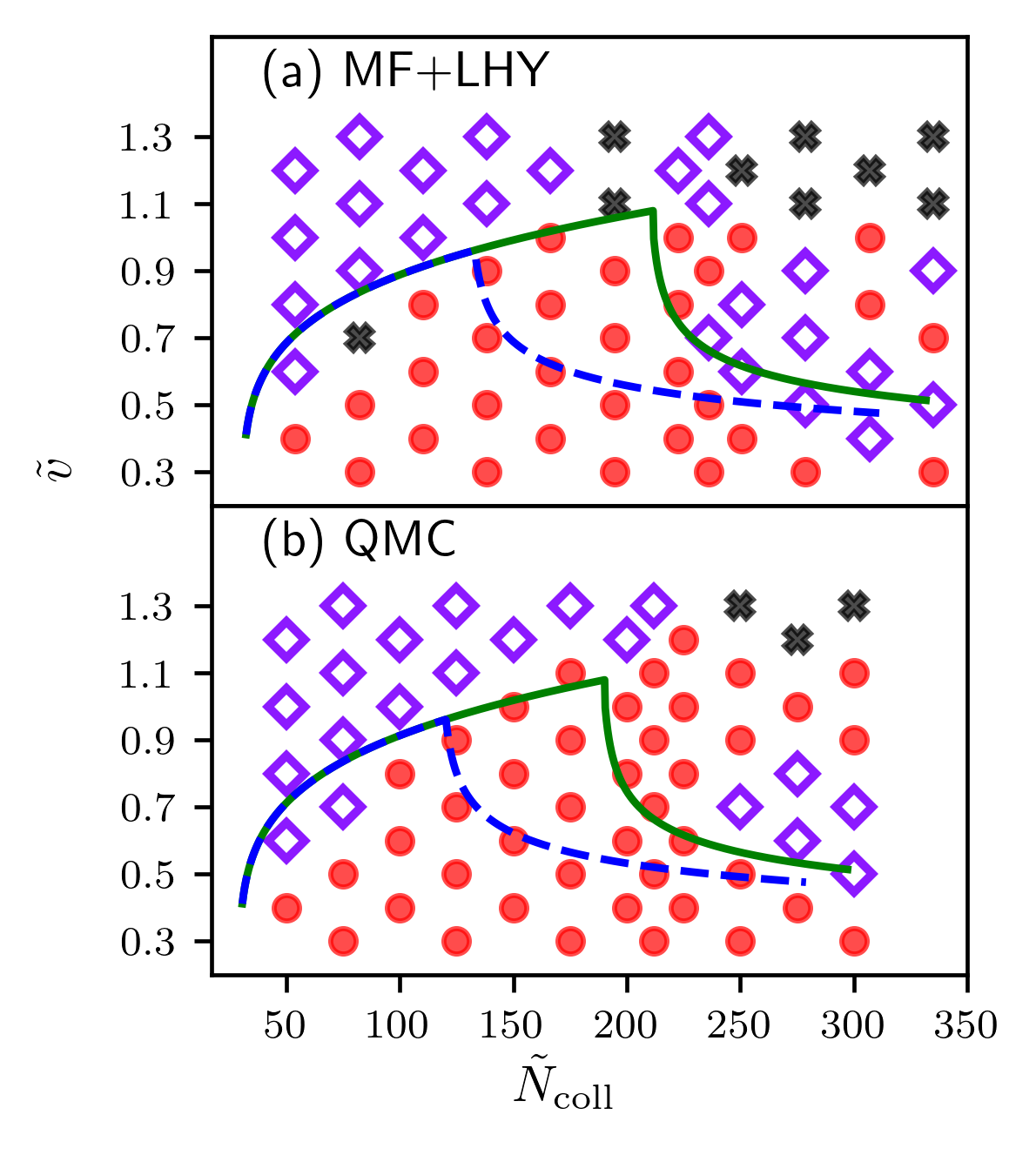
Figure 4: Collision outcomes obtained using the effective single-component MF+LHY (a) and QMC functional (b) with the scattering parameters corresponding to a magnetic field $B=56.23$ G (see Table 1). 3BL are not included. Atom number $N$ and velocity of each droplet at $t=0$ are re-scaled according to Eqs. (10) and (11), respectively. Red dots, purple diamonds and black crosses stand for merging, separation and evaporation collision outcome (see Fig. 3), respectively. Dashed blue and full green lines are the empirical fits to the experimental and MF+LHY results Ferioli et al. (2019), respectively, for the velocity threshold above (below) which the droplets separate (merge). QMC functional is given by Eq. (18) with parameters $\alpha=-0.812\hbar^{2}/(2ma_{11}^{5})$, $\beta=5.974\hbar^{2}/(2ma_{11}^{5-3\gamma})$ and $\gamma=1.276$, with $a_{11}=63.648a_{0}$.

V.2 Two-component calculations

We have performed collision simulations using the MF+LHY density functional in the two-component framework (Eqs. (16) and (17)). Notice that this is not possible with the present QMC functional, as it is written in terms of the total density alone. For each component, its wave function is evolved in time with the corresponding propagator (see Eqs. (14) and (22)).

We summarize in Fig. 5 the collision outcomes for several initial atom ratios $x$. The functional we use is that obtained from the scattering parameters $a_{ij}$ corresponding to the magnetic field $B=56.55$ G (see Table 1). In all cases the initial droplet separation is $d\approx 3500\,a_{11}\approx 9\,\xi$, where $\xi$ is the corresponding healing length (see Table 1). Since at $t=0$ the atom number ratio is not the optimal one, i.e., it does not correspond to the ground-state of the extended Gross-Pitaevskii approach, the initial profile of each droplet has been prepared as follows. Firstly, each droplet is equilibrated with optimal atom composition $x=1$ by means of imaginary-time propagation. Next, the real-time evolution is started and simultaneously the normalization of component 1 is changed to the desired value of $x$. When the collision is started with $x=1$ (Fig. 5a), the predictions within the two-component framework are in good agreement with calculations from Ref. Ferioli et al. (2019) but in poor agreement with experiment. As we decrease $x$, our results for the critical velocity are in better accord with the experimental results.

Note that there are small differences between the predictions obtained using effective single-component and two-component MF+LHY functionals assuming $x=1$. Since we are dealing with a finite system, the imposed requirement $\rho_{2}/\rho_{1}=\sqrt{a_{11}/a_{22}}$ satisfied in an effective single-component functional is not equally fulfilled in each spatial coordinate at the droplet surface in a two-component approach. Therefore, colliding drops display deviations of the density ratio $\rho_{2}/\rho_{1}$, which eventually leads to the difference in collision outcomes.

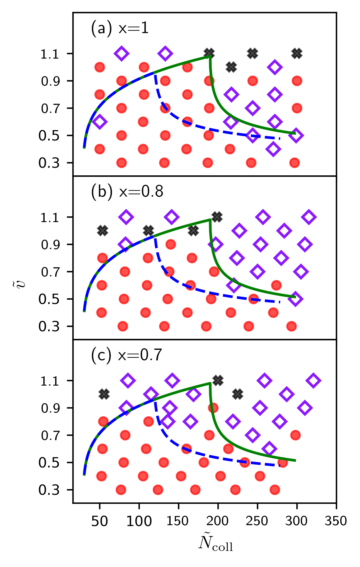
Figure 5: Collision outcome as a function of droplet velocity $\tilde{v}$ and total atom number evaluated at the instant of collision $\tilde{N}_{\rm coll}=\tilde{N}(t=t_{\rm coll})$ for the scattering parameters corresponding to $B=56.55$ G (see Table 1). Calculations are performed using two-component MF+LHY theory without including 3BL. Parameter $x=(N_{2}/N_{1})\sqrt{a_{22}/a_{11}}$ is the initial particle ratio at the beginning of collision. Points and lines have the same meaning as in Fig. 4.

Since $x\neq 1$ is not the equilibrium configuration, the atoms of the in-excess component are expelled out of the droplets as soon as time evolution starts. Therefore, the initial configuration is somewhat ill-prepared and the collision outcome depends on the initial distance $d$ between the two droplets (the larger the $d$, the larger the amount of atoms expelled from the droplets prior to colliding). Moreover, the evaporated atoms do not leave the collision region and may also influence the outcome. To highlight this important effect, we report in Fig. 6 the collision outcomes for non-equilibrated ($x=0.7$) droplets and two different initial distances. Starting the collision at a large distance $(d=45\xi)$, as in Fig. 6b, the prediction for the critical velocity coincides with that obtained within the effective single-component framework. This is quite a natural result meaning that, by the time the two droplets meet, they have already reached a quasi-equilibrium configuration where the ratio of atoms in each component corresponds to $x=1$.

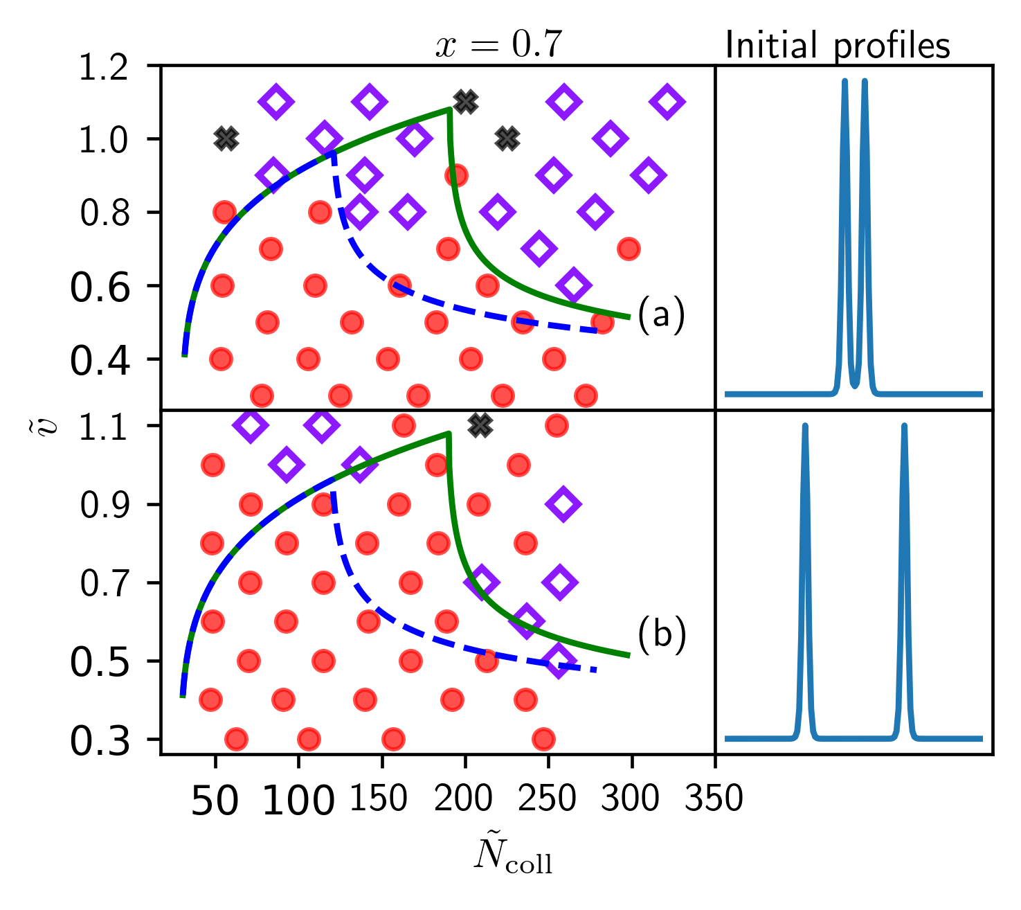
Figure 6: Same as Fig. 5 for the non-optimal atom number ratio $x=0.7$ and two different initial droplets distances. Left: Predictions of merging (red points), separation (purple diamonds) and evaporation (black crosses). Right: initial droplets density profiles along the approaching direction, $\rho(x,0,0;t=0)$. Full green and dashed blue lines have the same meaning as in Fig. 4. Initial droplet distances in panel (a) are the same as in Fig. 5c.

V.3 Effect of three-body losses and gas halo

We have also performed calculations including 3BL using the two-component MF+LHY density functional. Three-body recombination is assumed to be dominant in the $\ket{F,m_{F}}=\ket{1,0}$ channel, which we call state $1$ Ferioli et al. (2020); Semeghini et al. (2018). Consequently, in our simulations 3BL act only on $\psi_{1}$, Eq. (16).

We show in Fig. 7 the collision outcomes when the collision is started with the optimal atom number ratio $x=1$ (Fig. 7a) and with $x=0.8$ (Fig. 7b). The initial density profiles and the distance between the two droplets is the same as in Fig. 5. The scattering parameters $a_{ij}$ correspond to the magnetic field $B=56.55$ G (see Table 1). We choose a value of $K_{111}=2.73\times 10^{-28}{\rm cm}^{6}/{\rm s}=0.53\hbar/(m\xi^{2}\rho_{0}^{2})$, i.e., the same as in Ref. Ferioli et al. (2019), where it has been observed that the effective single-component theory, supplemented with a 3BL term $-i\hbar K\rho^{2}/2$, with $K=0.53\hbar/(m\xi^{2}\rho_{0}^{2})$ and $\rho$ being the total atom density, allowed to reproduce the experimental curve dividing merging from separation. Our calculations within two-component formalism show that only when the initial atom number ratio is non-optimal, namely $x=0.8$, we observe separation-like outcomes of the collision, and only in part of the phase diagram, for droplet velocities between $\tilde{v}=0.7$ and $\tilde{v}=1$.

We have also performed collisions using the effective single-component MF+LHY theory with the same value of three-body recombination as in Ref. Ferioli et al. (2019), $\tilde{K}=0.53$, and we find that the collision outcome (and thus the overall aspect of the $v-N$ phase diagram) is very sensitive to the initial preparation of the droplets, namely the distance and the atom number at the start of the collision. In a majority of collisions performed, we have observed separation of the droplets, followed by the evaporation, even for $(v,N)$ values for which merging is predicted in Ref. Ferioli et al. (2019). Thus, only a precise knowledge of how the droplets have been prepared (crucially, the initial droplet distance) would permit us to make a sensible comparison with the simulations of Ref. Ferioli et al. (2019).

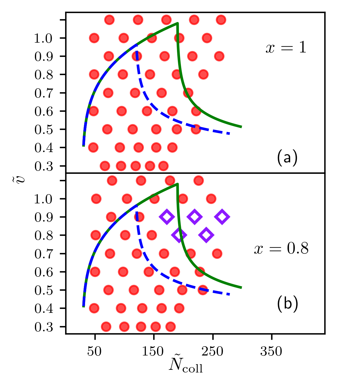
Figure 7: Same as Fig. (5). Merging (red points) and separation (purple diamonds) predicted within the two-component MF+LHY theory with 3BL included in the $\ket{F,m_{F}}=\ket{1,0}$ component using $K_{111}=2.73\times 10^{-28}cm^{6}/s$. Upper figure shows the predictions when the initial atom number ratio is $x=(N_{2}/N_{1})\sqrt{a_{22}/a_{11}}=1$, and the lower figure when $x=0.8$.

The droplet dynamics becomes even more complex if we allow for the initial non-optimal atom ratio. The collision outcome sensibly depends on three key parameters: i) initial droplet distance, ii) initial atom ratio, and iii) the value of the three-body losses coefficient. When we use a non-optimal atom ratio, we observe that the expelled atoms of the in-excess species form a gas halo enveloping the colliding droplets, thus acting as a kind of weakly repulsive buffer which slows the droplet relative velocity thus favoring merging over separation. Since the halo plays a role, we question the validity of the modeling of three-body losses since they just remove the atoms and energy from the simulation box.

To illustrate the effects of both the three-body losses and non-optimal atom ratios, we present in Fig. 8 four types of collisions obtained within the two-component MF+LHY functional. In all four cases, the integrated density $\rho_{i}(x,y)=\int dz\rho_{i}({\bm{r}})$ is shown, with component 1 (2) shown on the left (right).

In Fig. 8a and 8b, the time-evolution is shown without three-body losses present in the system. The droplets are prepared with non-optimal atom ratio $x=0.7$, as in Fig. 5. In both cases, separation is observed. For the smaller drops colliding at large velocity (Fig. 8a), drops evaporate upon separation since they require a minimum critical atom number to be self-bound Petrov (2015). When atom numbers are slightly higher (Fig. 8b), the remaining part of the drops separate. In both cases, there is a lot of evaporation in component 1 when the collision starts due to the initial population imbalance.

In Fig. 8c and 8d we present the influence of the initial atom ratio on the collisions with the included three-body coefficient $\tilde{K}_{111}=0.53$, for initial atom ratio equal to $x=1$ and $x=0.8$, respectively. In this case, the interplay of three-body losses and atom number imbalance leads to different geometries during the collision, which eventually yield different collision outcomes. When the initial atom ratio is $x=1$ (Fig. 8c), two protrusions are formed, reminiscent to collisions of He droplets Vicente et al. (2000); Escartín et al. (2019). The protrusions do not reach the size to be self-bound and eventually evaporate.

During the whole process, and more pronounced during the collision, when the central densities increase a lot, normalization of density 1 drops due to 3BL. This is followed by evaporation in component 2 by a mechanism of equilibration to optimal particle number, which creates a halo around the droplets. Around $t=30$ ms, a shock wave is formed in component 2, as a result of the interference of outward expansion of the droplet with the surrounding halo. Eventually, the shock wave passes through the halo, and the drops remain at place. This result highlights that evaporated atoms that remain around the colliding droplets contribute to the merging process. Indeed, it has been experimentally found that coalescence of viscous droplets can be facilitated when the collision region contains atoms in the gas phase Qian and Law (1997). Notice that in order for the droplets to merge, the gas between them must be expelled, which costs some energy favoring the merging.

When the collision is started with $x=0.8$ (Fig. 8d), evaporation of component 1 in the early stage of collision takes place. This happens due to equilibration towards optimal particle composition, which would happen even in the absence of 3BL (see Fig. 1). At about $t=25$ ms a different geometry and a thinner halo of species 2 atoms than in the case of $x(t=0)=1$ collision (Fig. 8c) is formed. This is due to the fact that in a time window when $x<1$, only the component 1 evaporates, not the component 2. The drops form a peanut-like configuration which has a much longer timelife, also observed in Ferioli et al. (2019), during which the large part of component 2 halo evaporates away. The peanut/cylinder eventually splits into two pieces due to surface tension. All of the separation collision outcomes observed in Fig. 7b are of the kind displayed in Fig. 8d, indicating that this could be a common feature for collisions with initial population imbalance and three-body losses present only in channel 111.

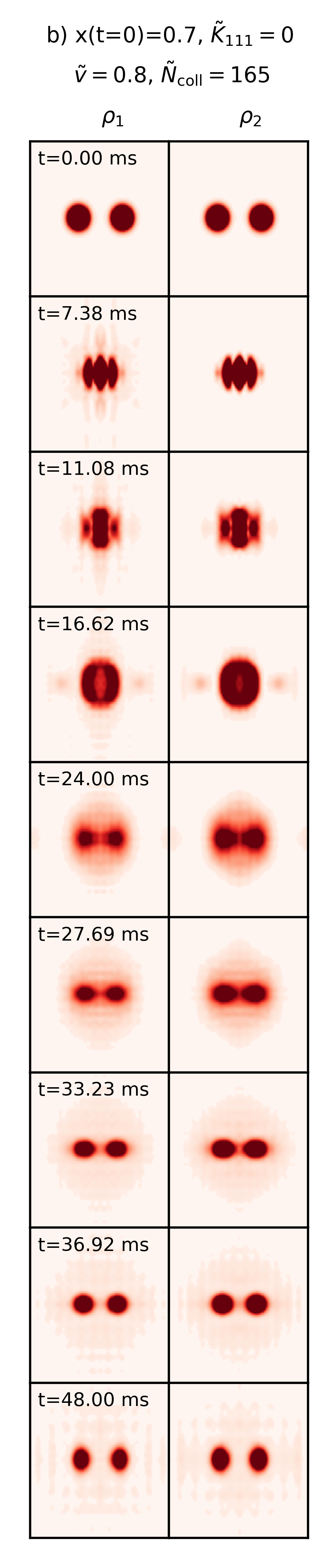
Figure 8: Images of the time evolution of $\rho_{i}=\int dz\rho_{i}({\bm{r}})$, for components $i=1$ and $2$, obtained within the two-component MF+LHY functional. The complete time-dependent evolution of the collisions is reported in Ref. material: Videos of the time-evolution of selected collisions .

VI Summary and conclusions

The recent study of head-on ³⁹K-³⁹K droplet collisions Ferioli et al. (2019) offers a new avenue of research by extending the study of quantum droplet collisions – previously restricted to the case of helium droplets Barranco et al. (2006) to much lower density and temperature ranges of ultra-dilute cold Bose gas mixtures. In the present work, we have theoretically reanalyzed this experiment by introducing elements not considered in the original work. In particular, we have improved the density functional approach by considering a functional based on QMC calculations that correctly incorporates the two relevant scattering parameters of the ³⁹K-³⁹K mixture, namely the $s$-wave scattering length and the effective range, as well as the most general version of a two-component equal-masses Bose-Bose energy functional. This two-component functional allows to introduce the 3BL only in the most affected component of the mixture, instead of in the total density of the system. This is a crucial improvement over the effective single-component functionals like QMC-based one, or the effective single-component MF+LHY functional which follows from the requirement that the two components of the mixture have the density ratio corresponding to the equilibrium one (the approach used in Ref. Ferioli et al. (2019)).

Our results can be summarized as follows:

(1) When 3BL are not considered, neither the QMC nor the effective single component MF+LHY approaches agree with experiment. As already noted in the theoretical analysis of Ref. Ferioli et al. (2019), the MF+LHY approach yields droplet merging at much higher velocities than observed experimentally. Moreover, the QMC-based and the single-component MF+LHY functionals meaningfully yield similar results. This is quite surprising since the QMC-based functional has a rather larger incompressibility and binding energy per atom than the single-component MF+LHY functional Cikojević et al. (2020), which was the reason to use it in this study.

(2) Given the experimental findings on the intensity of the 3BL in each component of the mixture Semeghini et al. (2018); Ferioli et al. (2020), it is not justified to let the 3BL act on both components, since it is about 100 times more effective in the component $\ket{F,m_{F}}=\ket{1,0}$ than in the other. There is little justification for using a single-component MF+LHY approach. When the value of the $K_{111}$ coefficient is in the range of those compatible with the experiments Ferioli et al. (2019), we find poor agreement with the experimental collision results. This implies that 3BL alone acting on equilibrated droplets cannot resolve the disagreement between the experiment and the results of either the effective single-component or the two-component MF+LHY approach, and we have been prompted to explore other natural possibilities.

(3) One of the possibilities is that droplets are not fully equilibrated when the collision is considered to have started. We completed our analysis assuming that the droplets are not in equilibrium at the start of the collision, including in some cases 3BL, always only in the component $\ket{F,m_{F}}=\ket{1,0}$.

If the droplets are not fully equilibrated when they enter the collision region, this affects the collision outcome because it introduces an important additional effect not previously considered, namely the halo of the expelled gaseous particles of the in-excess species that envelop the droplets and increase the tendency to merge. This effect has also been found in viscous droplet collisions Qian and Law (1997). Remarkably, the phase diagram changes even without the introduction of 3BL, as collisions between non-equilibrated droplets are shown to behave differently from equilibrated ones in terms of the optimal atom number ratio, leading to results that are in better agreement with experiment. We have focused here on zero temperature description, but it is plausible that thermally excited droplets Wang et al. (2020) could produce similar shifts in the critical velocity.

It is evident that the introduction of considerations of 3BL and/or non-equilibrium configuration at $t=0$ in the description of the collision process have a dramatic impact on the outcome of the simulations and add elements of difficult control when comparing with experiment.

Finally, we want to emphasize that while 3BL and non-equilibrium effects reduce the number of atoms and the kinetic energy in the colliding droplets, both effects are by no means equivalent. The term added to the functional to introduce 3BL takes atoms and energy out of the computational box, while the atoms of the in-excess component remain in the collision region and their presence may affect the collision outcome.