Different atom trapping geometries with time averaged adiabatic potentials

Abstract

In this article, we have theoretically studied the time averaged adiabatic potential (TAAP) scheme for realizing different atom trapping geometries. It is shown that by varying time orbiting potential (TOP) fields and radio frequency (rf) fields parameters, controlled manipulation of trapping potentials, and conversion from one trapping geometry to another, is possible. The proposed trapping geometries can be useful for studying various atom-optic phenomena such as Bose-Einstein condensation (BEC) in low dimensions, super-fluidity, tunnelling, atom interferometry, etc.

I Introduction

With the advent of laser cooling and trapping of atoms Metcalf (1999), the research in atomic physics has evolved in several dimensions from basic science Albiez et al. (2005); Ramanathan et al. (2011); Schumm et al. (2005) to practical applications Bertoldi et al. (2006); Peters et al. (2001); Müller et al. (2009) of cold atoms in quantum technologies Mark et al. (2011); Ryu et al. (2013); Alzar (2019). A magneto-optical trap (MOT) Wohlleben et al. (2001) is a work-horse device to produce samples of cold atoms for various studies and applications. The static magnetic traps Merloti et al. (2013); Chakraborty et al. (2016) and optical dipole traps Grimm et al. (2000) are widely used traps for further trapping and cooling of atoms from MOT to generate ultra-cold or degenerate atomic gas samples. In spite of a standard practice of using these magnetic and dipole traps for cold atoms, it is felt that a good handle on control and manipulation of trapping geometries can enrich our capabilities for use of cold atoms for several purposes. In this context, the rf-dressed adiabatic potential scheme, first proposed by Zobay and Garraway Zobay and Garraway (2001), has been implemented successfully to demonstrate atom trapping in different geometries Chakraborty and Mishra (2014); Heathcote et al. (2008); Zobay and Garraway (2001); Hofferberth et al. (2006); Sherlock et al. (2011). The rf-dressed magnetic traps Chakraborty and Mishra (2014); Chakraborty et al. (2016); Merloti et al. (2013); Easwaran et al. (2010) are able to generate some novel trapping geometries such as double well Schumm et al. (2005), ring trap Morizot et al. (2006); Heathcote et al. (2008); Sherlock et al. (2011), arc trap Chakraborty and Mishra (2014), etc, which are difficult to achieve by conventional static magnetic traps or laser dipole traps. These capabilities can be further enriched by use of Time Averaged Adiabatic Potential (TAAP) technique, which is an extension of the rf-dressed adiabatic potential technique and proposed by Lesanovsky and Klitzing Lesanovsky and von Klitzing (2007). In the TAAP scheme, a relatively lower frequency time averaging field, called time orbiting potential (TOP) Petrich et al. (1995) field, is applied on atoms in presence of rf and static magnetic fields used for rf-dressing. Gildemeister et al Gildemeister et al. (2012) have first experimentally demonstrated the working of atom trapping using TAAP scheme.

In this work, we have theoretically investigated various atom trapping geometries using TAAP scheme. Our results show that by varying the TOP fields parameters as well as rf-dressing fields parameters, various atom trapping geometries can be realized which are not possible with rf-dressing alone. In TAAP scheme, the conversion from one geometry to the other is possible. Some of these trapping geometries and their conversions can be used to study the dynamics of cold atoms and Bose-Einstein condensates Anderson et al. (1995); Davis et al. (1995) in low dimensions Merloti et al. (2013). Also, these trapping geometries can find applications in study of tunnelling Albiez et al. (2005); Schumm et al. (2005); Hofferberth et al. (2007), super-fluidity Ramanathan et al. (2011); Heathcote et al. (2008); Gildemeister et al. (2012), atom interferometry Kasevich and Chu (1991); Peters et al. (2001); Canuel et al. (2006); Carnal and Mlynek (1991), etc, which have applications in various atom-optic devices.

The article is organized as following. The section II presents the general theoretical frame work for description of rf-dressed adiabatic potentials and Time Averaged Adiabatic Potential (TAAP). In section III, we discuss our proposals for atom trapping geometries achievable using TAAP scheme along with the possibility of conversion from one geometry to the other. Finally, in section IV, we present the conclusion of our studies.

II Theory

When atoms are trapped in the static magnetic trap, the application of an rf-field results in the formation of new states, know as rf-dressed states. The energy eigen values corresponding to these dressed states are known as rf-dressed potentials (or adiabatic potentials). The rf-dressed potentials generally vary with position of the atom in the trap because of position dependent rf-field coupling strength inside the trap. Thus, atoms trapped in a magnetic trap in a particular magnetic hyperfine state can be transferred to a rf-dressed potential by exposing them to a rf-field of suitable frequency and amplitude Chakraborty et al. (2016). In the present theoretical work, we consider the quadrupole trap as a static magnetic trap with field variation given as

$$\textbf{B}_{\textbf{S}}(r)=B^{\prime}_{q}\begin{pmatrix}x\\ y\\ -2z\\ \end{pmatrix},$$ (1)

where $B^{\prime}_{q}$ is the quadrupole field gradient.

We take the rf-field of the form given by

$$\textbf{B}_{\textbf{rf}}(t)=\begin{pmatrix}B^{x}_{rf}\cos(\omega_{rf}t)\\ B^{y}_{rf}\cos(\omega_{rf}t+\phi^{y}_{rf})\\ B^{z}_{rf}\cos(\omega_{rf}t+\phi^{z}_{rf})\\ \end{pmatrix},$$ (2)

where $B^{x}_{rf}$, $B^{y}_{rf}$ and $B^{z}_{rf}$ are the amplitudes of the rf-field along $x$-, $y$- and $z$- directions respectively, and $\omega_{rf}$ is the angular frequency of the rf field. The parameters $\phi^{y}_{rf}$ and $\phi^{z}_{rf}$ are the phases of the $y$- and $z$-components of rf-field with respect to its $x$-component.

For an atom, in a state with hyperfine angular momentum F and interacting with the fields given by Eq. (1) and Eq. (2), the effective Hamiltonian in absence of any kinetic energy term can be written as

$$H_{eff}(r,t)=-\boldsymbol{\mu}.{\textbf{B}_{\textbf{eff}}(\textbf{r},t)}={\frac{g_{F}\mu_{B}}{\hbar}}{\textbf{F}.{\textbf{B}_{\textbf{eff}}(\textbf{r},t)}},$$ (3)

with

$$\textbf{B}_{\textbf{eff}}(\textbf{r},t)=\textbf{B}_{\textbf{S}}(\textbf{r})+\textbf{B}_{\textbf{rf}}(t)=\mid\textbf{B}_{\textbf{S}}(\textbf{r})\mid{\boldsymbol{\hat{e}}}_{S}+\textbf{B}_{\textbf{rf}}(t),$$ (4)

where $\hat{e}_{S}$ is the direction of the static magnetic field and $\boldsymbol{\mu}=-\frac{g_{F}\mu_{B}}{\hbar}\textbf{F}$ is the magnetic dipole moment of the atom having hyperfine angular momentum F.

For simplicity of calculations, a new co-ordinate system is chosen whose one of the axes coincides with the direction of quadrupole magnetic field. In this co-ordinate system, the static field vector becomes ${{(0,0,\mid\boldsymbol{B_{S}(r)}\mid)}^{T}}$, and the rf-field vector becomes ${(B_{rf}^{\perp 1}cos(\omega_{rf}t),B^{\perp 2}_{rf}cos(\omega_{rf}t+\gamma_{1}),B^{\parallel}_{rf}cos(\omega_{rf}t+\gamma_{2}))}^{T}$, where $\gamma_{1}$ and $\gamma_{2}$ are the relative phases of the field components in the new co-ordinate system. The hyperfine angular momentum is also changed to ${(F^{\perp 1},F^{\perp 2},F^{\parallel})}^{T}$. Now, if the Schrödinger wave equation is transformed in a rotating frame using an unitary operator described as $U=exp[i\omega_{rf}t(\frac{F^{\parallel}}{\hbar})]$, then the effective Hamiltonian in the rotating frame can be written as

$$H_{eff}^{R}(t)=UH_{eff}{U}^{\dagger}-i\hbar U\frac{\partial{U}^{\dagger}}{\partial t}=\frac{g_{F}{\mu}_{B}}{\hbar}\Big{[}F^{\parallel}B_{S}+F^{\parallel}B_{rf}^{\parallel}+\textbf{F}_{\textbf{R}}.\boldsymbol{{B}_{rf}^{\perp}}-\frac{\hbar\omega_{rf}}{g_{F}\mu_{B}}F^{\parallel}\Big{]},$$ (5)

where, $F^{\parallel}$ is the angular momentum along the static field direction. The parameter $\textbf{F}_{\textbf{R}}$ is the angular momentum perpendicular to the static field direction in the rotating frame. The components of $\textbf{F}_{\textbf{R}}$ can be written as ${F}_{R}^{\perp 1}=UF^{\perp 1}U^{\dagger}$ and ${F}_{R}^{\perp 2}=UF^{\perp 2}U^{\dagger}$.

The first term in Eq. (5) is the Zeeman energy term and second term involves the component of rf field along the static field. Second term has a vanishing contribution because $\mid\mu_{B}B_{rf}^{\parallel}\mid\ll\hbar{\omega}_{rf}$. After inserting the expression Gildemeister (2010) for $\textbf{F}_{\textbf{R}}$ and $\boldsymbol{{B}_{rf}^{\perp}}(t)$, and applying the rotating wave approximation, the expression for the effective Hamiltonian can be written as

$$H_{eff}^{R}=\frac{g_{F}{\mu}_{B}}{\hbar}\Big{[}F^{\parallel}\Big{(}B_{S}-\frac{\hbar\omega_{rf}}{g_{F}{\mu}_{B}}\Big{)}+\frac{F_{+}}{4}\Big{(}B_{rf}^{\perp 1}-iB_{rf}^{\perp 2}e^{i{\gamma}}\Big{)}+\frac{F_{-}}{4}\Big{(}B_{rf}^{\perp 1}+iB_{rf}^{\perp 2}e^{-i{\gamma}}\Big{)}\Big{]},$$ (6)

where $F_{+}=F^{\perp 1}+iF^{\perp 2}$ and $F_{-}=F^{\perp 1}-iF^{\perp 2}$ are the raising and lowering operator of hyperfine angular momentum in the rotated frame. $\gamma=\gamma_{2}-\gamma_{1}$ is the relative phase separation of the rf-field components in rotated co-ordinate system.

The eigenvalues of the Hamiltonian ($H_{eff}^{R}$), when solved in the basis of $|F,m_{F}\rangle$ states, leads to the expression for the rf-dressed adiabatic potential as

$$E_{AP}(r)=m_{F}\hbar\sqrt{{\Big{(}\frac{g_{F}\mu_{B}|\boldsymbol{B_{S}(r)}|}{\hbar}-{\omega}_{rf}}\Big{)}^{2}+\Big{(}\frac{g_{F}\mu_{B}}{2\hbar}\Big{)}^{2}\Big{[}{\Big{(}B_{rf}^{\perp 1}\Big{)}}^{2}+{\Big{(}B_{rf}^{\perp 2}\Big{)}}^{2}+2B_{rf}^{\perp 1}B_{rf}^{\perp 2}\sin(\gamma)\Big{]}}.$$ (7)

In a compact form, the adiabatic potential can be expressed as

$$E_{AP}(r)=m_{F}\hbar\sqrt{\mid{\Delta(r)\mid}^{2}+{|\Omega_{R}(r)|}^{2}},$$ (8)

where detuning ($\Delta$) and Rabi frequency ($\Omega_{R}$) for the dressing rf-field are expressed as

$$\Delta(r)=\frac{g_{F}{\mu}_{B}}{\hbar}|\boldsymbol{B_{S}(r)}|-\omega_{rf}.$$ (9)

and

$${|\Omega_{R}(r)|}^{2}={\Big{(}{\frac{g_{F}{\mu}_{B}}{2\hbar}}\Big{)}}^{2}\Big{[}{\Big{(}B_{rf}^{\perp 1}\Big{)}}^{2}+{\Big{(}B_{rf}^{\perp 2}\Big{)}}^{2}+2B_{rf}^{\perp 1}B_{rf}^{\perp 2}\sin(\gamma)\Big{]}.$$ (10)

Using the reverse transformation for fields, the expression for the Rabi frequency ($\Omega_{R}(r)$) in terms of field parameters in lab frame is given by

$${\mid\Omega_{R}(r)\mid}^{2}={\Big{(}\frac{{{g}_{F}{\mu}_{B}}}{2\hbar}\Big{)}}^{2}\Bigg{[}\frac{4{z}^{2}}{x^{2}+y^{2}+4{z}^{2}}\Bigg{(}\frac{{\Big{(}B_{rf}^{x}\Big{)}}^{2}{x}^{2}+{\Big{(}B_{rf}^{y}\Big{)}}^{2}{y}^{2}}{{x}^{2}+{y}^{2}}\Bigg{)}+\Bigg{(}\frac{{\Big{(}B_{rf}^{x}\Big{)}}^{2}{y}^{2}+{\Big{(}B_{rf}^{y}\Big{)}}^{2}{x}^{2}}{{x}^{2}+{y}^{2}}\Bigg{)}\\ +{\Big{(}B_{rf}^{z}\Big{)}}^{2}\Bigg{(}\frac{{x}^{2}+{y}^{2}}{{x}^{2}+{y}^{2}+4{z}^{2}}\Bigg{)}-\frac{2{B}_{rf}^{x}{B}_{rf}^{y}xy\cos({\phi}_{rf}^{y})}{{x}^{2}+{y}^{2}+4{z}^{2}}+\frac{4{B}_{rf}^{x}{B}_{rf}^{y}z\sin({\phi}_{rf}^{y})}{\sqrt{{x}^{2}+{y}^{2}+4{z}^{2}}}+\frac{4{B}_{rf}^{y}{B}_{rf}^{z}yz\cos({\phi}_{rf}^{y}-{\phi}_{rf}^{z})}{{x}^{2}+{y}^{2}+4{z}^{2}}\\ +\frac{2{B}_{rf}^{y}{B}_{rf}^{z}x\sin({\phi}_{rf}^{y}-{\phi}_{rf}^{z})}{\sqrt{{x}^{2}+{y}^{2}+4{z}^{2}}}+\frac{4{B}_{rf}^{z}{B}_{rf}^{x}xz\cos({\phi}_{rf}^{z})}{{x}^{2}+{y}^{2}+4{z}^{2}}+\frac{2{B}_{rf}^{z}{B}_{rf}^{x}y\sin({\phi}_{rf}^{z})}{\sqrt{{x}^{2}+{y}^{2}+4{z}^{2}}}\Bigg{]}.$$ (11)

From above expression (Eq. (8)) of adiabatic potential, it is evident that potential energy for atom trapping can be tailored to a large extent by choosing the phases ($\phi_{rf}^{y},\phi_{rf}^{z}$) and the amplitudes ($B_{rf}^{x},B_{rf}^{y},B_{rf}^{z}$) of the rf-fields.

The time averaged adiabatic potentials (TAAP) can be achieved by time averaging the rf-dressed or adiabatic potentials. This is achieved by applying the low frequency time orbiting potential (TOP) field in addition to dressing rf field to perform the time averaging.

The general expression of a TOP field is given as

$$\boldsymbol{B_{T}}(t)=B_{T}^{x}\sin(\omega_{T}t)\boldsymbol{\hat{e}}_{x}+B_{T}^{y}\sin(\omega_{T}t+\phi_{T}^{y})\boldsymbol{\hat{e}}_{y}+B_{T}^{z}\sin(\omega_{T}t+\phi_{T}^{z})\boldsymbol{\hat{e}}_{z},$$ (12)

where $B_{T}^{x}$, $B_{T}^{y}$ and $B_{T}^{z}$ are the magnitudes of TOP fields along $x$-,$y$- and $z$-directions respectively. The parameters $\phi_{T}^{y}$ and $\phi_{T}^{z}$ are the phases of the $y$- and $z$-components of TOP field with respect to the $x$- component.

In conventionally used TOP traps, a circularly polarized TOP field in the $x$-$y$ plane is used and its frequency ($\omega_{T}$) is very much greater than the frequency ($\omega_{r}$) of center of mass motion of the atom in quadrupole trap but very much lesser than the Larmor frequency ($\frac{g_{F}{\mu}_{B}B_{T}}{\hbar}$) provided by the TOP field. Mathematically the criteria can be written as

$$\omega_{r}\ll\omega_{T}<\frac{g_{F}{\mu}_{B}B_{T}}{\hbar},$$ (13)

where $B_{T}$ is the magnitude of the TOP field.

Finally, the most general expression Gildemeister et al. (2010) of time averaged adiabatic potential (TAAP) can be expressed as

$$E_{TAAP}(r)=\frac{\omega_{T}}{2\pi}\int_{0}^{\frac{2\pi}{\omega_{T}}}E_{AP}\Big{(}x+\frac{B_{T}^{x}}{{B}_{q}^{\prime}}\sin(\omega_{T}t),y+\frac{B_{T}^{y}}{{B}_{q}^{\prime}}\sin(\omega_{T}t+\phi_{T}^{y}),z+\frac{B_{T}^{z}}{2{B}_{q}^{\prime}}\sin(\omega_{T}t+\phi_{T}^{z})\Big{)}dt.$$ (14)

Here it is evident that by changing the TOP field parameters ($B_{T}^{x},B_{T}^{y},B_{T}^{z},\phi_{T}^{y},\phi_{T}^{z}$) and also the rf field parameters ($B^{x}_{rf},B^{y}_{rf},B^{z}_{rf},\phi^{y}_{rf},\phi^{z}_{rf}$), we can have several interesting atom trapping geometries. Some of these geometries are discussed in the following section.

III Results and discussion

Different atom trapping geometries under TAAP scheme can be achieved with choosing the rf-fields and TOP fields parameters appropriately. Using the TAAP scheme, a vertical ($z$-direction) double well trap was first demonstrated by Gildemeister et al Gildemeister et al. (2010) by choosing a vertical direction ($z$-direction) linearly polarized rf-field $\textbf{B}_{\textbf{rf}}(t)={(0,0,{B}_{rf}^{z}cos(\omega_{rf}t))}^{T}$ and a $x$-$y$ circularly polarized TOP field. Similarly, a ring type atom trap using TAAP scheme was first proposed by Lesanovsky et al Lesanovsky and von Klitzing (2007) and experimentally demonstrated by Sherlock et al Sherlock et al. (2011) by applying a circularly polarized rf-field in $x$-$y$ plane and $z$-direction linearly polarized TOP field. The double well trap is useful to study quantum tunneling Albiez et al. (2005) whereas a ring trap can be useful to study the persistent flow Heathcote et al. (2008); Ramanathan et al. (2011) of cold atomic gas and quantum degeneracy Sherlock et al. (2011) in low dimensions. A ring trap geometry is also useful for matter-wave interferometry Navez et al. (2016) with cold atoms which finds applications in developing atom-gyroscope Alzar (2019).

In this work, we have theoretically shown that the variation in rf-fields and TOP fields parameters can give rise to interesting TAAP traps for trapping of cold atoms in different geometries. We have considered that ${}^{87}Rb$ atoms are magnetically trapped in $|F=2,m_{F}=2\rangle$ hyperfine level of the ground state $5S_{1/2}$. In the calculations, we have chosen the quadrupole magnetic field with gradient of $B_{q}^{\prime}=$ $100$ G/cm and the rf-field of frequency $\omega_{rf}=$ $2\pi\times 1.5$ MHz. We have actually evaluated Eq. (14) to know the trap potential in TAAP scheme for different sets of rf and TOP fields parameters. The discussion on the obtained results is as follows.

III.1 Linearly polarized rf-field and TOP field modulations

Figure 1: (Color online) The conversion of a x-directional double well TAAP trap into a y-directional double well TAAP trap. The upper plots show the 3-D view of $25$ $\mu$K (intense red) and $35$ $\mu$K (light red) iso-potential surfaces, whereas lower plots show the 2-D contours of TAAP potentials for these geometries. The rf-field is linearly polarized in $x$-direction. TOP field is $y$-$z$ circularly polarized ($B_{T}^{y}$ = $B_{T}^{z}$ = $1.3$ G ) for figure (a). For plots (b) and (c) the TOP field is $x$-$z$ polarized with a phase difference of $\frac{\pi}{2}$ between $x$- and $z$- components. The double well gets oriented along $y$-direction for plot (c). The values of TOP fields for plot (b) are $B_{T}^{z}$ = $1.3$ G and $B_{T}^{x}=650$ mG, and for plot (c) are $B_{T}^{z}$ = $1.3$ G and $B_{T}^{x}=850$ mG. The other parameters are $B_{rf}^{x}=700$ mG, $\omega_{rf}=2\pi\times 1.5$ MHz, $\omega_{T}=2\pi\times 7$ kHz and ${{B}_{q}^{\prime}}=100$ G/cm.

It is known that the double well trap can be generated by using a linearly polarized rf-field and a circularly polarized TOP field in TAAP scheme Gildemeister et al. (2010). The polarization direction of rf-field has to be perpendicular to TOP field plane for getting the double well oriented along the direction of applied rf-field polarization. With this analogy, a $x$-directional double well can be generated by using a $x$-polarized rf-field and a $y$-$z$ circularly polarized TOP field. Using our simulations, we obtained these results which are shown in Fig. 1 (a) via three dimensional (3-D) and two-dimensional (2-D) iso-potential surfaces. We have further investigated that this $x$-directional double well trap can be changed to $y$-directional double well trap by changing only the TOP field configuration to $x$-$z$ polarized. The double well in $y$-direction clearly appears when $B_{T}^{x}$ is increased beyond a certain value for a fixed value of $B_{T}^{z}$. These results are shown in Fig. 1 (b) and (c). Here We note that in TAAP scheme, the orientation of double well can be changed by just controlling the TOP field parameters and without any change in rf-field configuration. Double well trap is considered useful for studying tunnelling Albiez et al. (2005) and matter-wave interference Schumm et al. (2005) phenomena. The well separation can be tuned by changing the rf-field frequency $\omega_{rf}$ and quadrupole field gradient ${{B}_{q}^{\prime}}$.

III.2 Circularly polarized rf-fields and TOP field modulations

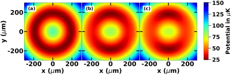
Figure 2: (Color online) The iso-potential contours of TAAP showing conversion of a ring type trapping potential into a double well along $y$-direction. The circularly polarized rf-field has $B_{rf}^{x}=B_{rf}^{y}=700$ mG. The value of $z$- TOP field ($B_{T}^{z}$) is $1.3$ G for plot (a). For plot (b), the Values of TOP field components are $B_{T}^{z}$ = $1.3$ G and $B_{T}^{x}=650$ mG, and for plot (c), $B_{T}^{z}$ = $1.3$ G and $B_{T}^{x}=850$ mG. The other parameters are $\omega_{rf}=2\pi\times 1.5$ MHz, $\omega_{T}=2\pi\times 7$ kHz and ${{B}_{q}^{\prime}}=100$ G/cm.

It is know from earlier studies Lesanovsky and von Klitzing (2007); Sherlock et al. (2011), as well as from simulations here, that a circularly polarized rf-field and a TOP field can give rise to a ring type atom trapping potential in TAAP scheme. For example, a $x$-$y$ circularly polarized rf-field and $z$-polarized TOP field results in a ring TAAP trap in $x$-$y$ plane. With further investigations, we have found that this ring trap can be converted to a $y$-directional double well trap by changing the $z$-polarized TOP field to $x$-$z$ polarized TOP field with a phase difference of $\frac{\pi}{2}$ between $x$- and $z$- components, as shown in Fig. 2. The value of phase between $x$- and $z$- components determines the orientation of the double well trap. Similarly, the $x$-$y$ circularly polarized rf-field and $y$-$z$ polarized TOP field can give rise to double well trap along $x$-axis as shown in Fig. 3. The above kind of conversions from ring to double well may be useful to study the dynamics of super-fluidity Ramanathan et al. (2011) and tunnelling Albiez et al. (2005) with the Bose-condensate of atoms.

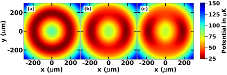
Figure 3: (Color online) The iso-potential contours of TAAP showing conversion of a ring type trapping potential into a double well along $x$-direction. The circularly polarized rf-field has $B_{rf}^{x}=B_{rf}^{y}=700$ mG. The value of $z$- TOP field ($B_{T}^{z}$) is $1.3$ G for plot (a). For plot (b), the values of TOP field components are $B_{T}^{z}$ = $1.3$ G and $B_{T}^{y}=650$ mG, and for plot (c), $B_{T}^{z}$ = $1.3$ G and $B_{T}^{y}=850$ mG. The other parameters are $\omega_{rf}=2\pi\times 1.5$ MHz, $\omega_{T}=2\pi\times 7$ kHz and ${{B}_{q}^{\prime}}=100$ G/cm.

III.3 Multiple rf-fields and TOP field modulations

Here we show that use of multiple rf-fields along with TOP fields results in different trapping potentials. For example, a circularly polarized rf-field in $x$-$y$ plane and a $z$-directional rf-field (along with $z$-TOP field) result in a potential minimum on an arc of the ring. The results are shown in Fig. 4(a). Further more, this arc type trapping potential can be converted into a $y$-directional double well when the $z$-TOP field is changed to a $x$-$z$ TOP field with a phase difference of $\frac{\pi}{2}$ between $x$- and $z$-components. These results are shown in Fig 4(b) and (c) where $B_{T}^{x}$ is given values of $650$ mG and $850$ mG for (b) and (c) respectively, and $B_{z}^{T}=1.3$ G is used for both plots (b) and (c). As shown in Fig. 4(c), the double well potential is better resolved when $B_{T}^{x}$ is given a higher value.

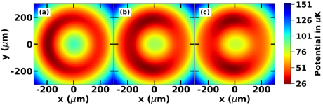
Figure 4: (Color online) The iso-potential contours of TAAP showing an arc type trapping potential and its further conversion into a $y$-directional double well trap. The $x$-$y$ circularly polarized rf-field with $B_{rf}^{x}=B_{rf}^{y}=700$ mG and a linearly $z$-polarized rf-field with $B_{rf}^{z}=300$ mG are considered. The value of $B_{T}^{z}$ is taken as $1.3$ G for all plots (a), (b) and (c). Only $z$-TOP field is considered for plot (a), where as $x$-$z$ TOP fields are considered for plots (b) and (c). The values of $B_{T}^{x}$ are $B_{T}^{x}=650$ mG for plot (b) and $B_{T}^{x}=850$ mG for plot (c). The other parameters are $\omega_{rf}=2\pi\times 1.5$ MHz, $\omega_{T}=2\pi\times 7$ kHz and ${{B}_{q}^{\prime}}=100$ G/cm.

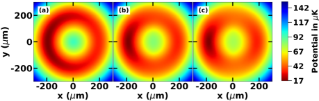
Figure 5: (Color online) The iso-potential contours of TAAP showing an arc type trapping potential and its further conversion into a $x$-directional asymmetric double well trap. The $x$-$y$ circularly polarized rf-field with $B_{rf}^{x}=B_{rf}^{y}=700$ mG and a linearly $z$-polarized rf-field with $B_{rf}^{z}=300$ mG are considered. The value of $B_{T}^{z}$ is taken as $1.3$ G for all plots (a), (b) and (c). Only $z$-TOP field is considered for plot (a), where as $y$-$z$ TOP fields are considered for plots (b) and (c). The values of $B_{T}^{y}$ are $B_{T}^{y}=650$ mG for plot (b) and $B_{T}^{y}=850$ mG for plot (c). The other parameters are $\omega_{rf}=2\pi\times 1.5$ MHz, $\omega_{T}=2\pi\times 7$ kHz and ${{B}_{q}^{\prime}}=100$ G/cm.

Similarly, an arc type of atom trap can be converted into an asymmetric $x$-directional double well when $z$-TOP field is changed to $y$-$z$ TOP field with a phase difference of $\frac{\pi}{2}$ between $y$- and $z$-components. These results are shown in Fig. 5. The $y$-direction TOP field component is increased and $z$-TOP field is kept at a fixed value. The separation between the wells is tunable by changing the rf field frequency $\omega_{rf}$ and quadrupole field gradient ${B}_{q}^{\prime}$.

An arc type of trap is useful for unequal population around the circumference of a ring. Rotation of an arc can be used to study superfluidity Ramanathan et al. (2011); Gupta et al. (2005) and atom interferometry Navez et al. (2016). When arc type geometry is getting converted into a asymmetric double well, this conversion can be used to split the atom cloud in an unequal proportion which is a suitable geometry for study of tunnelling Albiez et al. (2005).

IV Conclusion

We have theoretically shown various kinds of atom trapping geometries by using TAAP scheme. It is shown that TAAP scheme has versatility to design and manipulate the potential for atom trapping with appropriate combination of static magnetic field, rf-fields and TOP fields. Various conversions among TAAP geometries, such as conversions between different directional double well traps, from ring trap to double well trap and from an arc trap to double well trap, have been discussed. These conversions between different trapping geometries can be useful to study the quantum degeneracy in low dimensions, dynamics of atom traps, matter-wave interferometry, superfluidity and tunnelling.

V Acknowledgement

We acknowledge Kavish Bhardwaj for useful discussion and a careful reading of the manuscript. Sourabh Sarkar acknowledges the financial support by Raja Ramanna Centre for Advanced Technology, Indore under Homi Bhabha National Institute (HBNI) programme.

References

- Metcalf (1999) H. J. Metcalf, Laser Cooling and Trapping (Springer, 1999).
- Albiez et al. (2005) M. Albiez, R. Gati, J. Fölling, S. Hunsmann, M. Cristiani, and M. K. Oberthaler, Phys. Rev. Lett. 95, 010402 (2005), URL https://link.aps.org/doi/10.1103/PhysRevLett.95.010402.
- Ramanathan et al. (2011) A. Ramanathan, K. C. Wright, S. R. Muniz, M. Zelan, W. T. Hill, C. J. Lobb, K. Helmerson, W. D. Phillips, and G. K. Campbell, Phys. Rev. Lett. 106, 130401 (2011), URL https://link.aps.org/doi/10.1103/PhysRevLett.106.130401.
- Schumm et al. (2005) T. Schumm, S. Hofferberth, L. M. Andersson, S. Wildermuth, S. Groth, I. Bar-Joseph, J. Schmiedmayer, and P. Krüger, Nature Physics 1, 57 (2005), ISSN 1745-2481, URL https://doi.org/10.1038/nphys125.
- Bertoldi et al. (2006) A. Bertoldi, G. Lamporesi, L. Cacciapuoti, M. de Angelis, M. Fattori, T. Petelski, A. Peters, M. Prevedelli, J. Stuhler, and G. M. Tino, Eur. Phys. J. D 40, 271 (2006), URL https://doi.org/10.1140/epjd/e2006-00212-2.
- Peters et al. (2001) A. Peters, K. Y. Chung, and S. Chu, Metrologia 38, 25 (2001), URL https://doi.org/10.1088%2F0026-1394%2F38%2F1%2F4.
- Müller et al. (2009) T. Müller, M. Gilowski, M. Zaiser, P. Berg, C. Schubert, T. Wendrich, W. Ertmer, and E. M. Rasel, Eur. Phys. J. D 53, 273 (2009), URL https://doi.org/10.1140/epjd/e2009-00139-0.
- Mark et al. (2011) M. J. Mark, E. Haller, K. Lauber, J. G. Danzl, A. J. Daley, and H.-C. Nägerl, Phys. Rev. Lett. 107, 175301 (2011), URL https://link.aps.org/doi/10.1103/PhysRevLett.107.175301.
- Ryu et al. (2013) C. Ryu, P. W. Blackburn, A. A. Blinova, and M. G. Boshier, Phys. Rev. Lett. 111, 205301 (2013), URL https://link.aps.org/doi/10.1103/PhysRevLett.111.205301.
- Alzar (2019) C. L. G. Alzar, AVS Quantum Sci. 1, 014702 (2019), URL https://doi.org/10.1116/1.5142003.
- Wohlleben et al. (2001) W. Wohlleben, F. Chevy, K. Madison, and J. Dalibard, Eur. Phys. J. D 15, 237 (2001), URL https://doi.org/10.1007/s100530170171.
- Merloti et al. (2013) K. Merloti, R. Dubessy, L. Longchambon, A. Perrin, P.-E. Pottie, V. Lorent, and H. Perrin, New Journal of Physics 15, 033007 (2013), URL https://doi.org/10.1088/1367-2630/15/3/033007.
- Chakraborty et al. (2016) A. Chakraborty, S. R. Mishra, S. P. Ram, S. K. Tiwari, and H. S. Rawat, Journal of Physics B: Atomic, Molecular and Optical Physics 49, 075304 (2016), URL https://doi.org/10.1088%2F0953-4075%2F49%2F7%2F075304.
- Grimm et al. (2000) R. Grimm, M. Weidemüller, and Y. B. Ovchinnikov (Academic Press, 2000), vol. 42 of Advances In Atomic, Molecular, and Optical Physics, pp. 95 – 170, URL http://www.sciencedirect.com/science/article/pii/S1049250X0860186X.
- Zobay and Garraway (2001) O. Zobay and B. M. Garraway, Phys. Rev. Lett. 86, 1195 (2001), URL https://link.aps.org/doi/10.1103/PhysRevLett.86.1195.
- Chakraborty and Mishra (2014) A. Chakraborty and S. R. Mishra, Journal of the Korean Physical Society 65, 1324 (2014), URL https://doi.org/10.3938/jkps.65.1324.
- Heathcote et al. (2008) W. H. Heathcote, E. Nugent, B. T. Sheard, and C. J. Foot, New Journal of Physics 10, 043012 (2008), URL https://doi.org/10.1088%2F1367-2630%2F10%2F4%2F043012.
- Hofferberth et al. (2006) S. Hofferberth, I. Lesanovsky, B. Fischer, J. Verdu, and J. Schmiedmayer, Nature Physics 2, 710 (2006), URL https://doi.org/10.1038/nphys420.
- Sherlock et al. (2011) B. E. Sherlock, M. Gildemeister, E. Owen, E. Nugent, and C. J. Foot, Phys. Rev. A 83, 043408 (2011), URL https://link.aps.org/doi/10.1103/PhysRevA.83.043408.
- Easwaran et al. (2010) R. K. Easwaran, L. Longchambon, P.-E. Pottie, V. Lorent, H. Perrin, and B. M. Garraway, Journal of Physics B: Atomic, Molecular and Optical Physics 43, 065302 (2010), URL https://doi.org/10.1088%2F0953-4075%2F43%2F6%2F065302.
- Morizot et al. (2006) O. Morizot, Y. Colombe, V. Lorent, H. Perrin, and B. M. Garraway, Phys. Rev. A 74, 023617 (2006), URL https://link.aps.org/doi/10.1103/PhysRevA.74.023617.
- Lesanovsky and von Klitzing (2007) I. Lesanovsky and W. von Klitzing, Phys. Rev. Lett. 99, 083001 (2007), URL https://link.aps.org/doi/10.1103/PhysRevLett.99.083001.
- Petrich et al. (1995) W. Petrich, M. H. Anderson, J. R. Ensher, and E. A. Cornell, Phys. Rev. Lett. 74, 3352 (1995), URL https://link.aps.org/doi/10.1103/PhysRevLett.74.3352.
- Gildemeister et al. (2012) M. Gildemeister, B. E. Sherlock, and C. J. Foot, Phys. Rev. A 85, 053401 (2012), URL https://link.aps.org/doi/10.1103/PhysRevA.85.053401.
- Anderson et al. (1995) M. H. Anderson, J. R. Ensher, M. R. Matthews, C. E. Wieman, and E. A. Cornell, Science 269, 198 (1995), ISSN 0036-8075, eprint https://science.sciencemag.org/content/269/5221/198.full.pdf, URL https://science.sciencemag.org/content/269/5221/198.
- Davis et al. (1995) K. B. Davis, M. O. Mewes, M. R. Andrews, N. J. van Druten, D. S. Durfee, D. M. Kurn, and W. Ketterle, Phys. Rev. Lett. 75, 3969 (1995), URL https://link.aps.org/doi/10.1103/PhysRevLett.75.3969.
- Hofferberth et al. (2007) S. Hofferberth, B. Fischer, T. Schumm, J. Schmiedmayer, and I. Lesanovsky, Phys. Rev. A 76, 013401 (2007), URL https://link.aps.org/doi/10.1103/PhysRevA.76.013401.
- Kasevich and Chu (1991) M. Kasevich and S. Chu, Phys. Rev. Lett. 67, 181 (1991), URL https://link.aps.org/doi/10.1103/PhysRevLett.67.181.
- Canuel et al. (2006) B. Canuel, F. Leduc, D. Holleville, A. Gauguet, J. Fils, A. Virdis, A. Clairon, N. Dimarcq, C. J. Bordé, A. Landragin, et al., Phys. Rev. Lett. 97, 010402 (2006), URL https://link.aps.org/doi/10.1103/PhysRevLett.97.010402.
- Carnal and Mlynek (1991) O. Carnal and J. Mlynek, Phys. Rev. Lett. 66, 2689 (1991), URL https://link.aps.org/doi/10.1103/PhysRevLett.66.2689.
- Gildemeister (2010) M. Gildemeister, Ph.D. thesis, University of Oxford (2010).
- Gildemeister et al. (2010) M. Gildemeister, E. Nugent, B. E. Sherlock, M. Kubasik, B. T. Sheard, and C. J. Foot, Phys. Rev. A 81, 031402 (2010), URL https://link.aps.org/doi/10.1103/PhysRevA.81.031402.
- Navez et al. (2016) P. Navez, S. Pandey, H. Mas, K. Poulios, T. Fernholz, and W. von Klitzing, New Journal of Physics 18, 075014 (2016), URL https://doi.org/10.1088/1367-2630/18/7/075014.
- Gupta et al. (2005) S. Gupta, K. W. Murch, K. L. Moore, T. P. Purdy, and D. M. Stamper-Kurn, Phys. Rev. Lett. 95, 143201 (2005), URL https://link.aps.org/doi/10.1103/PhysRevLett.95.143201.