Double transitions and hysteresis in heterogeneous contagion processes

Abstract

In many real-world contagion phenomena, the number of contacts to spreading entities for adoption varies for different individuals. Therefore, we study a model of contagion dynamics with heterogeneous adoption thresholds. We derive mean-field equations for the fraction of adopted nodes and obtain phase diagrams in terms of the transmission probability and fraction of nodes requiring multiple contacts for adoption. We find a double phase transition exhibiting a continuous transition and a subsequent discontinuous jump in the fraction of adopted nodes because of the heterogeneity in adoption thresholds. Additionally, we observe hysteresis curves in the fraction of adopted nodes owing to adopted nodes in the densely connected core in a network.

I Introduction

The spread of information, fads, rumors, innovations, or diseases has significantly increased globally because of the development of communication and mobility technologies goffman1964 ; daley1964 ; granovetter1978 ; may1991 ; pastor2001 ; watts2002 ; pastor2015 . To understand and control the spreading phenomena, quantitative modeling of contagion processes is crucial pastor2015 ; centola2018 . Contagion processes can be divided into two classes based on the type of contacts with active neighbors: simple and complex contagions kermack1927 ; harris1974 ; may1991 ; granovetter1978 ; centola2007 ; centola2010 . Simple contagion is a contagion process with independent interactions between the inactive and the active may1991 . Compartmental epidemic models such as the susceptible-infected-recovered may1991 ; kermack1927 ; newman2002 and susceptible-infected-susceptible models may1991 ; pastor2001 are examples of the simple contagion model. In contrast, complex contagion consists of collective interactions among active neighbors watts2002 ; centola2007 ; chae2015 ; dual2018 . Compared to the simple contagion, complex contagion processes are controlled by group interaction; that is, the probability of adoption strongly depends on the number of contacts with active neighbors. Multiple contacts to spreading entities are required for adoption in the complex contagion. Various social and biological spreading models such as threshold model granovetter1978 ; watts2002 ; gleeson2007 ; lee2014 , generalized epidemic model janssen2004 ; choi2018 ; baek2019 , diffusion percolation adler1988 , and bootstrap percolation chalupa1979 ; adler1991 ; baxter2010 are examples of the complex contagion model.

Recently, there have been several attempts for unifying simple and complex contagion processes dodds2004 ; cellai2011 ; baxter2011 ; karampourniotis2015 ; czaplicka2016 ; wang2016 ; min2018 . Empirical data of the spread of social behavior in a social networking services (SNS) indicate that adoption thresholds for different individuals are heterogeneous, depending on the characteristics of agents dow2013 ; state2015 . A unified contagion model incorporates different number of contacts to a spreading entity required for adoption, similar to the heterogeneity of adoptability observed in empirical data min2018 . In particular, while some agents change their state in contagion processes immediately after the first contact to new information following simple contagion, others require multiple contacts for adoption following complex contagion state2015 . According to the observations, real-world contagion phenomena are neither simple nor complex contagions, but they could be a mixture of the two, with different adoption thresholds for different agents. Because the characteristics of individuals significantly vary in reality, the heterogeneity of adoption threshold can be widespread for many contagion phenomena. In addition, such a unified contagion model can be useful for analyzing the spread of epidemics of multiple interacting pathogens because interacting epidemics is indistinguishable from social complex contagion janssen2016 ; min2020 ; hebert2020 . Therefore, generalized contagion processes integrating simple and complex contagions are of importance.

Here, we study a model of contagion dynamics on random networks with heterogeneous adoption thresholds for different agents. Although some previous works have also considered heterogeneous adoption thresholds  dodds2004 ; cellai2011 ; baxter2011 ; karampourniotis2015 ; czaplicka2016 ; wang2016 ; min2018 , most of them have assumed that adopted individuals acquired permanent adoption. In reality, many adopted individuals can lose their adopted state and return to the pool of susceptible individuals. In our model, we have added a transition from the adopted state back to susceptible state in contrary to previous studies pastor2001 ; majdandzic2014 . The process is implemented autonomously for each agent, similar to the recovery process in the classical susceptible-infected-susceptible model may1991 ; pastor2001 . In our study, we have added both heterogeneous adoption thresholds for each individual and also recovery process. Incorporating the heterogeneity and recovery process, we find a double phase transition with an intermediate phase in which nodes following simple contagion are adopted but nodes with complex contagion remain susceptible. In addition, we find hysteresis curves in the fraction of adopted nodes with respect to the contact probability. Our study provides the simple mechanism of hysteresis majdandzic2014 ; min2014 ; chen2017 and multiple phase transition colomer2014 ; allard2017 ; min2018 in contagion processes on complex networks.

II Model

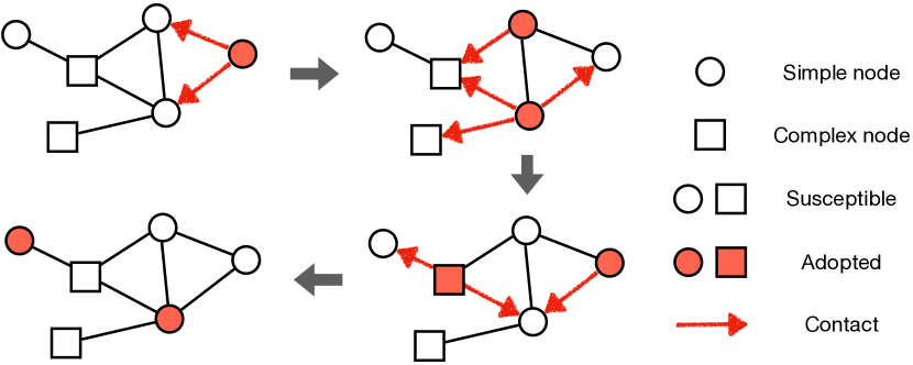
Figure 1: An example of our model with simple and complex nodes. Susceptible nodes (open symbols) are adopted when the number of contacts to the adopted is equal or larger than its assigned adoption threshold, either $n=1$ for simple nodes (circles) or $n=2$ for complex nodes (squares). Adopted nodes become susceptible in the next time step.

First, we consider a network with $N$ nodes that can be either susceptible or adopted. Thereafter, we assign adoption threshold $\theta_{i}$ for node $i$, which represents the number of contacts required to change their state from susceptible to adopted. When $\theta_{i}=1$, node $i$ is adopted after a single contact with an adopted neighbor at each time step according to simple contagion (simple nodes). When $\theta_{i}>1$, it corresponds to complex contagion, indicating that multiple contacts are required for adoption at each time step (complex nodes). For simplicity, in this study, we assume that all complex nodes in a network have an adoption threshold of $\theta=n$. That is, the fraction $p$ of nodes are complex nodes with an adoption threshold of $n$, and the others $1-p$ are simple nodes. The fraction $p$ of complex nodes represents the degree of the heterogeneity in adoption thresholds.

An example of the proposed model is presented in Fig. 1. The circles (squares) represent simple (complex) nodes and open (filled) symbols represent susceptible (adopted) nodes. Initially, the fraction $R_{0}$ of the nodes is adopted, and the others are susceptible. In our model, the dynamics is in discrete time steps. At each time step, each pair of connected nodes contacts each other with a contact probability $\lambda$. If the number of contacts with adopted neighbors is equal or larger than its adoption threshold, the node becomes adopted at the next time step. Contacts for adoption repeat for all nodes in a network. All adopted nodes become the susceptible state, which can be adopted again, like the recovery process in susceptible-infected-susceptible model. Note that an adopted node can remain adopted at the next time step if the number of contacts to its adopted neighbors is equal or larger than its adoption threshold. The adoption and recovery processes are repeated until a steady state is reached. In the steady state, the system is in either an absorbing or an active phase. In the absorbing phase, all nodes in a network are susceptible, and there is no more contagion dynamics. In contrast, a finite fraction of nodes remain in the adopted state in the active phase, which is the source of active dynamics. To assess the steady-state behavior, we measure the fraction $R$ of adopted nodes. While $R=0$ for the absorbing phase, $R$ is a nonzero value for the active phase.

The followings are the three important parameters of the model: contact probability $\lambda$, fraction $p$ of the complex nodes, and adoption threshold $n$ of the complex nodes. The contact probability $\lambda$ represents how often each connected pair interacts with each other, the fraction of complex nodes represents the degree of heterogeneous adoptability, and the adoption threshold $n$ represents the stubbornness of the complex nodes to adopt. We measure the fraction $R$ of the adopted nodes in a steady state based on three parameters, $\lambda$, $p$, and $n$.

III Analytical approach

To predict the final fraction of adopted nodes, we derive heterogeneous mean-field equations, assuming a locally tree-like network in the limit $N\rightarrow\infty$. Because there are two classes of nodes in a network, we consider two types of node degrees: the number of links connected to the simple $k_{s}$ and complex $k_{c}$ neighbors. Additionally, we define $s_{k_{s},k_{c}}^{t}$ and $c_{k_{s},k_{c}}^{t}$ as the fraction of the adopted simple and complex nodes with degrees $k_{s}$ and $k_{c}$, respectively, at time $t$. We define the probability that a randomly chosen node pointing to a simple (complex) node is an adopted one as $\phi_{s}^{t}$ ($\phi_{c}^{t}$). For a random network without any degree-degree correlations, the probabilities $\phi_{s}^{t}$ and $\phi_{c}^{t}$ can be expressed as follows:

$$\phi_{s}^{t} =\sum_{k_{s},k_{c}}\frac{k_{s}P(k_{s},k_{c})}{\langle k_{s}\rangle}s_{k_{s},k_{c}}^{t},$$ (1)

$$\phi_{c}^{t} =\sum_{k_{s},k_{c}}\frac{k_{c}P(k_{s},k_{c})}{\langle k_{c}\rangle}c_{k_{s},k_{c}}^{t},$$ (2)

where $P(k_{s},k_{c})$ is the distribution of the joint degree for $k_{s}$ and $k_{c}$ of a network.

The fraction of adopted simple nodes $s_{k_{s},k_{c}}^{t+1}$ can be calculated according to the following equations gleeson2007 ; min2018

$$s_{k_{s},k_{c}}^{t+1} =1-(1-\lambda\phi_{s}^{t})^{k_{s}}(1-\lambda\phi_{c}^{t})^{k_{c}}.$$ (3)

The terms $(1-\lambda\phi_{s}^{t})^{k_{s}}$ and $(1-\lambda\phi_{s}^{t})^{k_{s}}$ stand for the probability that a node does not contact with adopted simple and adopted complex neighbors, respectively. Similarly, the fraction of the adopted complex nodes can be obtained by

$$c_{k_{s},k_{c}}^{t+1} =1-\sum_{\mu=0}^{n-1}\sum_{\mu_{s}=0}^{\mu}\binom{k_{s}}{\mu_{s}}(\lambda\phi_{s}^{t})^{\mu_{s}}(1-\lambda\phi_{s}^{t})^{k_{s}-\mu_{s}}$$

$$\times \binom{k_{c}}{\mu-\mu_{s}}(\lambda\phi_{c}^{t})^{\mu-\mu_{s}}(1-\lambda\phi_{c}^{t})^{k_{c}-(\mu-\mu_{s})}.$$ (4)

The term $\sum_{\mu}\cdots$ represents the probability that the number $\mu$ of contacts to adopted neighbors is less than the adoption threshold $n$. Note that if adopted nodes are again adopted by their neighbors, they remain adopted at the next time step as Eqs. 3 and 4 imply.

We can derive the following self-consistency equations in the limit $t\rightarrow\infty$ combining Eqs. 1-4:

$$\phi_{s}^{\infty} =1-\sum_{k_{s},k_{c}}\frac{k_{s}P(k_{s},k_{c})}{\langle k_{s}\rangle}(1-\lambda\phi_{s}^{\infty})^{k_{s}}(1-\lambda\phi_{c}^{\infty})^{k_{c}},$$ (5)

$$\phi_{c}^{\infty} =1-\sum_{k_{s},k_{c}}\frac{k_{c}P(k_{s},k_{c})}{\langle k_{c}\rangle}\sum_{\mu=0}^{n-1}\sum_{\mu_{s}=0}^{\mu}\binom{k_{s}}{\mu_{s}}\binom{k_{c}}{\mu-\mu_{s}}$$ (6)

$$\times(\lambda \phi_{s}^{\infty})^{\mu_{s}}(1-\lambda\phi_{s}^{\infty})^{k_{s}-\mu_{s}}(\lambda\phi_{c}^{\infty})^{\mu-\mu_{s}}(1-\lambda\phi_{c}^{\infty})^{k_{c}-(\mu-\mu_{s})}.$$

We can obtain $\phi_{s}^{\infty}$ and $\phi_{c}^{\infty}$ by solving the coupled equations iteratively from the initial values of $\phi_{s}$ and $\phi_{c}$. Putting them into Eqs. 3-4, the fraction of the adopted simple and complex nodes in the steady state, $s_{k_{s},k_{c}}^{\infty}$, and $c_{k_{s},k_{c}}^{\infty}$, can be obtained. Finally, the average fraction $R$ of adopted nodes in the steady state with the fraction $p$ of complex nodes can be obtained by

$$R=\sum_{k_{s},k_{c}}P(k_{s},k_{c})\left[pc_{k_{s},k_{c}}^{\infty}+(1-p)s_{k_{s},k_{c}}^{\infty}\right].$$ (7)

The fraction $R$ of the adopted nodes can be calculated from the fixed points in Eqs. 1 and 2. The trivial solution of $R$ with $\phi_{s}^{\infty}=\phi_{c}^{\infty}=0$ corresponds to an absorbing phase where $R=0$. An active phase with $R>0$ can appear when $\phi_{c}$ or $\phi_{c}$ is nonzero. The largest eigenvalue, $\Lambda$, of the Jacobian matrix $\mathcal{J}$ in Eqs. 1 and 2 identifies the stability of a fixed point $\vec{\phi}=(\phi_{s}^{*},\phi_{c}^{*})$ by applying a linear stability analysis. Specifically, the fixed point $(\phi_{s}^{*},\phi_{c}^{*})$ is stable when $\Lambda(\vec{\phi})>1$. Note that multiple stable fixed points of $\vec{\phi}$ can appear for a certain set of parameters.

A simple condition of the transition between the absorbing and active phases is that $\Lambda$ at $(\phi_{s},\phi_{c})=(0,0)$ is equal to unity. Since the Jacobian matrix $\mathcal{J}$ at $(\phi_{s},\phi_{c})=(0,0)$ is given by

$$\mathcal{J}=\begin{pmatrix}\lambda\frac{\langle k_{s}^{2}\rangle}{\langle k_{s}\rangle}&\lambda\frac{\langle k_{s}k_{c}\rangle}{\langle k_{s}\rangle}\\ 0&0\end{pmatrix},$$ (8)

this condition leads to the transition point for a given $p$

$$\lambda_{1}=\frac{\langle k_{s}\rangle}{\langle k_{s}^{2}\rangle}.$$ (9)

If $\lambda>\lambda_{1}$, the system reaches the active phase ($R>0$) initiated by adopted simple nodes. When all the nodes are simple nodes, we can recover the epidemic threshold for the susceptible-infected-susceptible model pastor2001 ; pastor2015 . There can be transition points $\lambda_{2}$ other than $(\phi_{s},\phi_{c})=(0,0)$. Unfortunately, we cannot express $\lambda_{2}$ in a closed form expression but the transitions can be identified by numerical integrations with the condition $\Lambda(\vec{\phi})=1$ for the non-zero solution of $\vec{\phi}=(\phi_{s}^{*},\phi_{c}^{*})$. It is not feasible to obtain $\lambda_{2}$ in a closed form because the non-zero fixed points $\vec{\phi}=(\phi_{s}^{*},\phi_{c}^{*})$ cannot be simply reduced into an analytical expression. Also note that these transitions at $\lambda_{2}$ cause the abrupt change of $R$ between low $R$ and high $R$ rather than the transition between the absorbing and active phases.

IV Results

IV.1 Phase diagram on Erdös-Rényi graphs

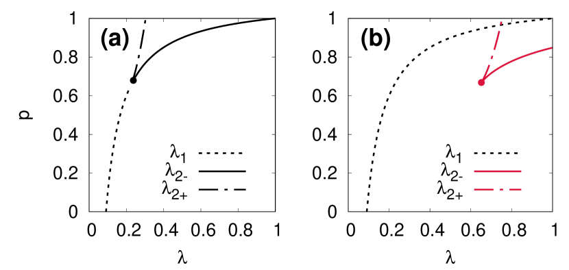
Figure 2: Phase diagram of a heterogeneous contagion model with (a) $n=2$ and (b) $n=5$ for ER networks with $z=10$. Continuous transition lines $\lambda_{1}$ are indicated by dashed lines. Discontinuous transitions are indicated by dot-dashed lines $\lambda_{2+}$ and solid lines $\lambda_{2-}$. Critical points where the discontinuous jump disappears are indicated by filled circles.

We consider the contagion model with heterogeneous adoption thresholds on Erdös-Rényi (ER) networks. Degree distribution of the ER graphs in the thermodynamic limit $N\rightarrow\infty$ is approximately given by a Poisson distribution $P(k)=e^{-z}z^{k}/k!$, where $z$ denotes the average degree. We assume that simple and complex nodes are distributed randomly on a network. Thereafter, $P(k_{s},k_{c})$ can be decomposed into the product of two Poisson distributions, $P(k_{s})$ and $P(k_{c})$, with average degrees of $(1-p)z$ and $pz$, respectively. With the setting, the transition $\lambda_{1}$ is located at

$$\lambda_{1}=\frac{1}{(1-p)z+1}.$$ (10)

We examine the phase diagram with $n=2$ on ER networks with $z=10$ [Fig. 2(a)]. First, we observe a continuous (dashed) transition line, as predicted by Eq. 10. The transition becomes discontinuous, denoted by $\lambda_{2-}$ (solid), when the fraction $p$ of the complex nodes exceeds the critical point $(\lambda_{c},p_{c})$. In addition when $p>p_{c}$, another discontinuous transition line appeared, denoted by $\lambda_{2+}$ (dot-dashed). Our theory predicts that these three transition lines meet at a single point, $(\lambda_{c},p_{c})$. When $p$ is less than the point, there is only a continuous transition between the absorbing and active phases like a typical absorbing phase transition. However, there are two transition lines, $\lambda_{2-}$ and $\lambda_{2+}$ when $p$ is larger than $p_{c}$. When the contagion dynamics begins from a tiny fraction of adopted seeds, that is $R_{0}\approx 0.01$, the theory predicts the location of the transition at $\lambda_{2-}$. However, when the fraction initially adopted nodes is sufficiently high, that is $R_{0}\approx 0.99$, the transition takes place on $\lambda_{2+}$.

A phase diagram with $n=5$ is shown in Fig. 2(b) as a typical example of $n>2$. We find qualitatively similar phase diagram for all $n>2$. We observe a continuous phase transition line $\lambda_{1}$, as predicted by Eq. 10. In addition, we observe two additional discontinuous transition lines, $\lambda_{2+}$ (dot-dashed) and $\lambda_{2-}$ (solid), when $p$ is larger than the critical point $p_{c}$, denoted by a filled circle. Note that the discontinuous transition line $\lambda_{2-}$ is separated from $\lambda_{1}$. When $p<p_{c}$, a single transition point $\lambda_{1}$ is observed, meaning that the systems change from absorbing to active phase at $\lambda_{1}$. When $p>p_{c}$, a continuous transition line $\lambda_{1}$ and two discontinuous transitions lines, $\lambda_{2-}$ and $\lambda_{2+}$, are observed. Depending on the initial seed fraction, $R_{0}$, a discontinuous transition is realized at different points, either $\lambda_{2-}$ or $\lambda_{2+}$. Specifically, when dynamics starts with low $R_{0}$, the fraction $R$ of the adopted nodes abruptly changes at $\lambda_{2-}$. However when contagion processes starts with high $R_{0}$, the transition appears at $\lambda_{2+}$ and not $\lambda_{2-}$.

We conduct Monte-Carlo simulations of the contagion dynamics on ER networks with $N=10^{4}$ and $z=10$ for $n=5$ with various $p$ values, averaged over $10^{4}$ independent runs in order to verify our theory. We find that the system reaches a steady state where the fraction $R$ of adopted nodes does not change significantly over time, after the initial transient period. We measure the fraction of adopted nodes $R$ at the steady state. In this example, the dynamics starts with a few fractions of adopted seeds such as $R_{0}\approx 0.01$. As shown in Fig. 3(a), numerical results (symbols) are consistent with the theory (lines). As the fraction $p$ of the complex nodes increases, the transition point $\lambda_{1}$ delays as predicted by theory. In addition, when $p>p_{c}$ where $p_{c}=0.668$ for $n=5$, an additional transition can appear at $\lambda_{2-}$. Note that $\lambda_{2+}$ is inaccessible with the choice of initial condition.

IV.2 Double transitions

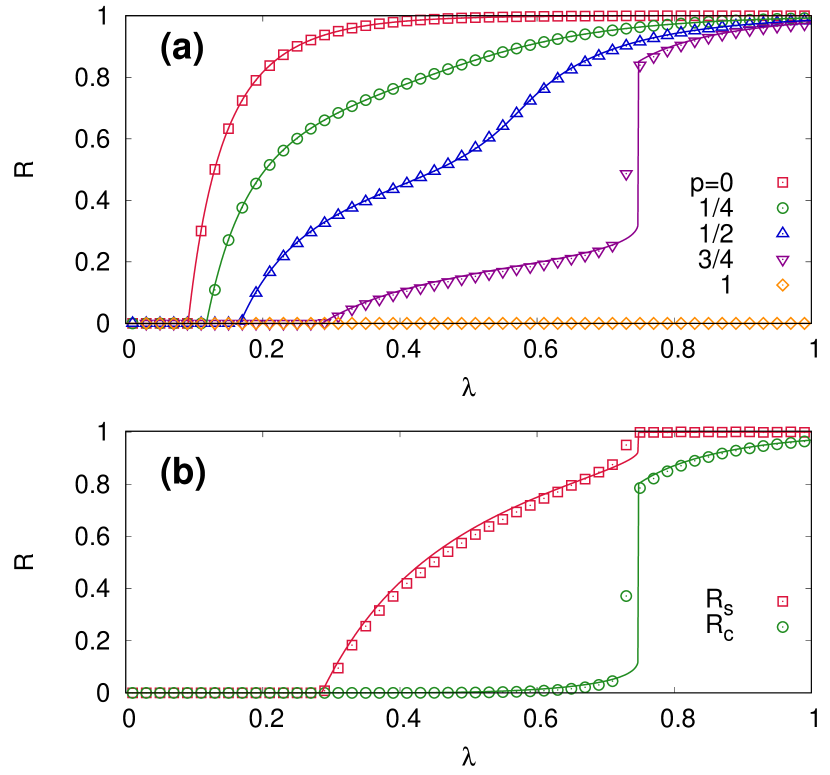
Figure 3: (a) Fraction $R$ of the adopted nodes as a function of $\lambda$ for different $p$ with $n=5$, $R_{0}\approx 0.01$, on ER networks with $N=10^{4}$, and $z=10$, averaged over $10^{4}$ independent runs. (b) Fraction of adopted simple nodes $R_{s}$ (squares) and complex nodes $R_{c}$ (circles) as a function of $\lambda$ with $p=3/4$. In the intermediate phase, $R_{s}$ increases gradually whereas most complex nodes remain susceptible (low $R_{c}$). Numerical simulations (symbols) and theoretical calculation (lines) are shown together.

Let us examine the contagion dynamics with $n=5$ and $p=3/4$, which is $p>p_{c}$. As shown in Fig. 3(a), we have two consecutive transitions, $\lambda_{1}$ and $\lambda_{2-}$, which are called a double transition colomer2014 ; allard2017 ; min2018 . The transition between the absorbing and active phases takes place at $\lambda_{1}$. In addition, the fraction $R$ of the adopted nodes that are already non-zero suddenly increases at $\lambda_{2-}$ with a discontinuous jump in $R$. There is an intermediate phase between the two transitions, where $R$ is non-zero but still low. In this model, we show that the double phase transitions can naturally appear because of the heterogeneity of the adoption thresholds. For social contagions, it is often more realistic to use the threshold as the relative fraction of contacts to adopted nodes out of the total number of neighbors rather than the absolute number of contacts to the adopted granovetter1978 ; watts2002 . We observed that the double phase transitions also appear when we use the threshold given by the fraction of adopted nodes (see appendix).

We measure the fraction of adopted nodes with simple contagion $R_{s}$ and complex contagion $R_{c}$ with $p=3/4$ to demonstrate the mechanism of the double phase transition [Fig. 3(b)]. Here, $R_{s}$ ($R_{c}$) represents the fraction of the adopted simple (complex) nodes for all simple (complex) nodes. For instance, $R_{s}=0$ when all the simple nodes are susceptible, and $R_{s}=1$ when all the simple nodes are adopted. In an absorbing phase $\lambda<\lambda_{1}$, all nodes are susceptible regardless of being simple or complex nodes, leading to $R=0$. At $\lambda_{1}$, simple nodes start to be adopted. However, most complex nodes remain susceptible (low $R_{c}$) until $\lambda<\lambda_{2-}$. Therefore, simple nodes are adopted whereas most complex nodes are susceptible in the intermediate phase, $\lambda_{1}<\lambda<\lambda_{2-}$. At the second transition $\lambda_{2-}$, complex nodes collectively change their state from susceptible to adoption, leading to a discontinuous jump in $R_{c}$. As a result, when $\lambda>\lambda_{2-}$, most nodes, either simple or complex, are adopted. Therefore, both $R_{s}$ and $R_{c}$ show a high value with a discontinuous jump at $\lambda_{2-}$.

IV.3 Hysteresis curves

Moreover, we show the implication in two discontinuous transition lines, $\lambda_{2-}$ and $\lambda_{2+}$, above $p_{c}$ [see Fig. 2(b)]. There are two different $R$ in a steady state between two transition lines, meaning that $\lambda_{2+}<\lambda<\lambda_{2-}$. As shown in Fig. 4, there is a bistable region with two stable $R$, for instance, $\lambda\approx 0.8$. We defined two loci of stable $R$ as $R_{+}$ (circles) and $R_{-}$ (squares). While we can obtain the upper locus, $R_{+}$, when contagion dynamics starts with a high $R_{0}$, we can arrive at the lower locus, $R_{-}$, when $R_{0}$ is low. Depending on the initial fraction of the seed nodes, the locations of the transition point where a discontinuous jump appears is also different, either $\lambda_{2+}$ for $R_{+}$ or $\lambda_{2-}$ for $R_{-}$. Here we use ER networks with $N=10^{4}$, $z=10$ for $n=5$ and $p=0.8$ over $10^{4}$ independent runs in our numerical simulations. And, the dynamics starts with a fractions of adopted seeds $R_{0}\approx 0.01$ for $R_{-}$ and $R_{0}\approx 0.99$ for $R_{+}$.

Because of bistability, there can be hysteretic behavior in the fraction $R$ of the adopted nodes by varying $\lambda$. If the transmission probability increases from low $\lambda$, the system sustains the intermediate phase where simple nodes are adopted but most complex nodes remain susceptible until $\lambda_{2-}$. At $\lambda_{2-}$, $R$ suddenly increases because of the adoption of complex nodes. But when the system reaches high $R$ phase, the phase maintains for $\lambda_{2+}<\lambda<\lambda_{2-}$. To regain the low $R$ phase, $\lambda$ must be less than $\lambda_{2+}$.

We search for the origin of hysteretic behavior based on the topology of a network. We first assign the $k$-core (also known as the $k$-shell) index for each node to assess the coreness dorogovtsev2006 . Here, $k$-core represents a subset of nodes formed by iterative removal of all nodes with degree less than $k$. That is, the $k$-core is a maximal set of nodes where all nodes have at least $k$ degrees within the set. The procedure to assign $k$-core index is as follows: i) First, assign $k$-core index to each node as $k_{co}=1$. ii) Remove all nodes with remaining degree $k\leq k_{co}$, iteratively. iii) Increase $k$-core index by one to all remaining nodes. iv) Repeat ii) and iii) until all nodes are removed. Thereafter, a unique value of $k_{co}$ is assigned for each node. The $k$-core index assigned represents the coreness of each node in the topology of a network.

.

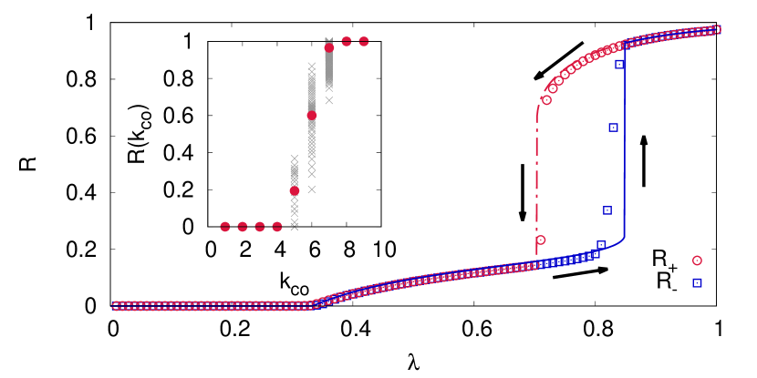
Figure 4: The fraction of adopted nodes $R$ as a function of $\lambda$ for ER graphs with $N=10^{4}$, $z=10$, $n=5$, and $p=0.8$. We find the bistable region where two stable $R$, $R_{+}$ and $R_{-}$, exist between the two transitions, $\lambda_{2+}$ and $\lambda_{2-}$. Numerical simulations (symbols) and theoretical calculation (lines) are shown. (inset) The fraction of the adopted complex nodes at $\lambda=0.8$, following $R_{+}$ curve averaged over nodes with the same $k$-core index $k_{co}$ (filled circles). Gray symbols represent the probability that a node with $k_{co}$ is adopted and obtained for each node averaged in time.

We measure the average fraction $R(k_{co})$ of the adopted complex nodes as a function of the $k$-core index $k_{co}$ in the bistable region, that is, $p=0.8$. The inset of Fig. 4 shows $R(k_{co})$ in the upper locus, $R_{+}$. We find that nodes with a high $k$-core index can be in the adopted state for $R_{+}$, implying that the complex nodes in the core of a network can collectively sustain the active state. Additionally, once high $k$-core nodes in $R_{+}$ become susceptible, $R$ remains at a low value until a group of complex nodes collectively change their state to be adopted at $\lambda_{2-}$.

V Discussion

Here, we study a model of contagion dynamics with heterogeneous adoption thresholds for different agents. In addition, we incorporate a recovery process from adopted to susceptible state. We find a double transition, which is a continuous transition from the absorbing to active phases and a subsequent discontinuous jump in the fraction of the adopted nodes. The double transition occurs with an intermediate phase in which simple nodes are adopted but complex nodes remain susceptible. Moreover, we find hysteresis in the fraction of the adopted nodes with respect to the contact probability. Our study sheds light on some fundamental aspects of the mechanism of hysteresis in contagion processes and multiple phase transitions in complex networks. For more realistic modeling it would be also interesting to investigate these factors that we has not covered in this study: the influence of heterogeneity in degree distributions such as scale-free networks and/or the existence of degree-degree correlations, to name a few.

*

Appendix A Threshold Model

It is often more realistic to define the threshold as the relative fraction of adopted nodes out of the total number of neighbors rather than the number of adopted nodes, in particular for social contagions granovetter1978 ; watts2002 . In order to validate the robustness of our main finding, we check the case with the threshold defined by the fraction of contacts to adopted nodes. To be specific, for complex node $i$, when the fraction of contacts to adopted nodes is equal or larger than a certain threshold $\eta$, node $i$ becomes adopted. We assume as previous that the fraction $p$ of nodes are complex nodes with an adoption threshold of $\eta$ for the fraction of adopted contacts, and the others $1-p$ are simple nodes.

For the case, we can derive the similar equations with Eqs. 1-4 with the following modification of $c_{k_{s},k_{c}}$:

$$c_{k_{s},k_{c}}^{t+1} =1-\sum_{\mu=0}^{\mu/(k_{s}+k_{c})<\eta}\sum_{\mu_{s}=0}^{\mu}\binom{k_{s}}{\mu_{s}}(\lambda\phi_{s}^{t})^{\mu_{s}}(1-\lambda\phi_{s}^{t})^{k_{s}-\mu_{s}}$$

$$\times \binom{k_{c}}{\mu-\mu_{s}}(\lambda\phi_{c}^{t})^{\mu-\mu_{s}}(1-\lambda\phi_{c}^{t})^{k_{c}-(\mu-\mu_{s})}.$$ (11)

Then, by using Eq. 7, we can obtain the fraction of adopted nodes in the steady state with the threshold given by the fraction. We also conduct numerical simulations of the dynamics on ER networks with $N=10^{4}$ and $z=10$ for $\eta=1/2$, $R_{0}\approx 0.01$ with various $p$ values, averaged over $10^{2}$ independent runs. As shown in Fig. 5, numerical results (symbols) are well consistent with the theory (lines). In addition, the double phase transitions are observed for the threshold given by the fraction of adopted nodes.

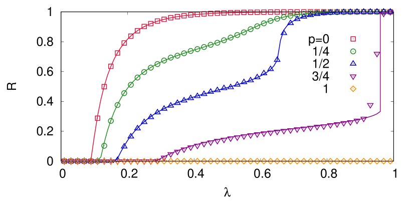
Figure 5: Fraction $R$ of the adopted nodes as a function of $\lambda$ for different $p$ with $\eta=1/2$, $R_{0}\approx 0.01$, on ER networks with $N=10^{4}$ and $z=10$, averaged over $10^{2}$ independent runs.

References

- (1) W. Goffman and V. Newill, Generalization of epidemic theory: An application to the transmission of ideas, Nature 204, 4955 (1964).
- (2) D. J. Daley and D. G. Kendall, Epidemics and rumors, Nature 204, 4963 (1964).
- (3) M. Granovetter, Threshold models of collective behavior, Am. J. Social. 83, 1420 (1978).
- (4) R. M. May and R. M. Anderson, Infectious disease of humans: dynamics and control, Oxford University Press (1991).
- (5) R. Pastor-Satorras and A. Vespignani, Epidemic spreading in scale-free networks, Phys. Rev. Lett. 86, 3200 (2001).
- (6) D. J. Watts, A simple model of global cascades on random networks, Proc. Natl. Acad. Sci. 99, 5766 (2002).
- (7) R. Pastor-Satorras, C. Castellano, P. Van Mieghem, and A. Vespignani, Epidemic processes in complex networks, Rev. Mod. Phys. 87, 925 (2015).
- (8) D. Centola, How behavior spreads: The science of complex contagions, Princeton University Press (2018).
- (9) W. O. Kermack and A. G McKendrick, A contribution to the mathematical theory of epidemics, Proc. Royal Soc. London A 115, 700 (1927).
- (10) T. E. Harris, Contact interactions on a lattice, Ann. Probab. 2, 969 (1974).
- (11) D. Centola and M. Macy, Complex contagions and the weakness of long ties, Am. J. Social. 113, 702 (2007).
- (12) D. Centola, The spread of behavior in an online social network experiment, Science 329, 1194 (2010).
- (13) M. E. J. Newman, Spread of epidemic disease on networks, Phys. Rev. E 66, 016128 (2002).
- (14) H. Chae, S.-H. Yook, and Y. Kim, Discontinuous phase transition in a core contact process on complex networks, New J. Phys. 17, 023039 (2015).
- (15) B. Min and M. San Miguel, Competition and dual users in complex contagion processes, Sci. Rep. 8, 14580 (2018).
- (16) J. P. Gleeson and D. J. Cahalane, Seed size strongly affects cascades on random networks, Phys. Rev. E 75, 056103 (2007).
- (17) K.-M. Lee, C. D. Brummitt, and K.-I. Goh, Threshold cascades with response heterogeneity in multiplex networks, Phys. Rev. E 90, 062816 (2014).
- (18) H.-K. Janssen, M. Müller, and O. Stenull, Generalized epidemic process and tricritical dynamic percolation, Phys. Rev. E 70, 026114 (2004).
- (19) W. Choi, D. Lee, J. Kertész, and B. Kahng, Two golden times in two-step contagion models: A nonlinear map approach, Phys. Rev. E 98, 012311 (2018).
- (20) Y. Baek, Role of hubs in the synergistic spread of behavior, Phys. Rev. E 99, 020301(R) (2019).
- (21) J. Adler and A. Aharony, Diffusion percolation: 1. Infinite time limit and bootstrap percolation, J. Phys. A 21, 1387 (1988).
- (22) J. Chalupa, P. L. Leath, and G. R. Reich, Bootstrap percolation on a Bethe lattice, J. Phys. C 12, L31 (1979).
- (23) J. Adler, Bootstrap percolation, Physica A 17, 453 (1991).
- (24) G. J. Baxter, S. N. Dorogovtsev, A. V. Goltsev, and J. F. F. Mendes, Bootstrap percolation on complex networks, Phys. Rev. E 82, 011103 (2010).
- (25) P. S. Dodds and D. J. Watts, Universal behavior in a generalized model of contagion, Phys. Rev. Lett. 92, 218701 (2004).
- (26) D. Cellai, A. Lawlor, K. A. Dawson, and J. P. Gleeson, Tricritical point in heterogeneous -core percolation, Phys. Rev. Lett. 107, 175703 (2011).
- (27) G. J. Baxter, S. N. Dorogovtsev, A. V. Goltsev, and J. F. F. Mendes, Heterogeneous -core versus bootstrap percolation on complex networks, Phys. Rev. E 83, 051134 (2011).
- (28) P. D. Karampourniotis, S. Sreenivasan, B. K. Szymanski, and G. Korniss, The impact of heterogeneous thresholds on social contagion with multiple initiators, Plos One 10, e0143020 (2015).
- (29) A. Czaplicka, R. Toral, and M. San Miguel, Competition of simple and complex adoption on interdependent networks, Phys. Rev. E 94, 062301 (2016).
- (30) W. Wang, M. Tang, P. Shu, and Z. Wang, Dynamics of social contagions with heterogeneous adoption thresholds: crossover phenomena in phase transition, New J. Phys. 18, 013029 (2016).
- (31) B. Min and M. San Miguel, Competing contagion processes: complex contagion triggered by simple contagion, Sci. Rep. 8, 10422 (2018).
- (32) P. A. Dow, L. Adamic, and A. Friggeri, The anatomy of large Facebook cascades, ICWSM 1, 12 (2013).
- (33) B. State and L. Adamic, The diffusion of support in an online social movement: evidence from the adoption of equal-sign profile pictures, Proc. 18th ACM Conf. Comput. Supported Cooperat. Work Social Comput. 1741 (2015).
- (34) H.-K. Janssen and O. Stenull, First-order phase transitions in outbreaks of co-infectious diseases and the extended general epidemic process, EPL (Europhys. Lett.) 113, 26005 (2016).
- (35) B. Min and C. Castellano, Message-passing theory for cooperative epidemics, Chaos 30(2), 023131 (2020).
- (36) L. Hébert-Dufresne, S. V. Scarpino, and J.-G. Young, Macroscopic patterns of interacting contagions are indistinguishable from social reinforcement, Nat. Phys. 16, 426-431 (2020).
- (37) A. Majdandzic, B. Podobnik, S. V. Buldyrev, D. Y. Kenett, Spontaneous recovery in dynamical networks, S. Havlin, and H. E. Stanley, Nat. Phys. 10, 34-38 (2014).
- (38) B. Min and K.-I. Goh, Multiple resource demands and viability in multiplex networks, Phys. Rev. E 89, 040802(R) (2014).
- (39) L. Chen, F. Ghanbarnejad, D. Brockmann, Fundamental properties of cooperative contagion processes, New J. Phys. 19, 103041 (2017).
- (40) P. Colomer-de-Simón and M. Boguñá, Double percolation phase transition in clustered complex networks, Phys. Rev. X 4, 041020 (2014).
- (41) A. Allard, B. M. Althouse, S. V. Scarpino, L. Hébert-Dufresne Asymmetric percolation drives a double transition in sexual contact networks, Proc. Natl. Acad. Sci. 114, 8969 (2017).
- (42) S. N. Dorogovtsev, A. V. Goltsev, J. F. F. Mendes, -core organization of complex networks, Phys. Rev. Lett. 96, 040601 (2006).