A single formula for the law of the wall and its application to wall-modelled large-eddy simulation

Abstract

In this work, we propose a single formula for the law of the wall, which is dubbed as the logarithmic-exponential (LOG-EXP) formula, for predicting the mean velocity profile in different regions near the wall. And then a feedforward neural network (FNN), whose inputs and training data are based on this new formula, is trained for the wall-modelled large-eddy simulation (WMLES) of turbulent channel flows. The direct numerical simulation (DNS) data of turbulent channel flows is used to evaluate the performance of both the formula and the FNN. Compared with the Werner-Wengle (WW) model for the WMLES, a better performance of the FNN for the WMLES is observed for predicting the Reynolds stresses.

I Introduction

The law of the wall is one of the cornerstones in wall-bounded turbulent flows Pope (2001); Davidson (2015). Different formulae have been proposed in the literature for the law of the wall. Roughly, they can be divided into two groups, i.e., the piecewise formulae and the single formulae. In the early year, the piecewise function was developed to describe the dynamics in different near-wall regions of the inner layer (e.g., for turbulent channel flows, it is located in the range of $0\leq y\leq 0.1\delta$, where y denotes the wall-normal direction and $\delta$ is the half-height of the channel) Prandtl (1910); Taylor (1916); Kármán (1939); Deissler (1954); Rannie (1956); Breuer and Rodi (1996); Werner and Wengle (1993); Inagaki et al. (2002), which includes the viscous sublayer, the buffer layer and the logarithmic layer Pope (2001). The most widely used law of the wall describes the viscous sublayer using the linear profile, i.e.,

$$U^{+}=y^{+},$$ (1)

where $U^{+}=U/u_{\tau}$, $y^{+}=y/\delta_{v}$ with the friction velocity $u_{\tau}=\sqrt{\tau_{w}/\rho}$ (where $\tau_{w}$ is the wall shear stress and $\rho$ is the fluid density) and the viscous scale $\delta_{v}=\nu/u_{\tau}$ ($\nu$ is the kinematic viscosity of the fluid), and the logarithmic layer using the logarithmic law, i.e.,

$$U^{+}=\frac{1}{\kappa}\ln\left(y^{+}\right)+5.0,$$ (2)

where $\kappa=0.4$ is the Kármán constant. A list of different piecewise formulae proposed in the literature for the law of the wall is shown in Table 1. There are two disadvantages of the piecewise formulae: 1) the velocity in the buffer layer is not accurately described; 2) the velocity derivative is discontinuous because of the piecewise nature of these formulae. To resolve these two issues, different types of the law of the wall based on single formula have been proposed in the literature, which are often of two forms, i.e., the analytical form Reichardt (1951); Spalding (1961); Rasmussen (1975); Musker (1979); Dean (1976); Monkewitz, Chauhan, and Nagib (2007) and the numerical form Van Driest (1956); Duprat et al. (2011). The analytical forms are usually complicated or do not have a sound prediction Spalding (1961); Musker (1979); Dean (1976); Monkewitz, Chauhan, and Nagib (2007), while the numerical forms have a better prediction of the velocity profile Van Driest (1956); Duprat et al. (2011), but do not have a clear physical meaning or difficult to use in practice. Different single formulae for the law of the wall proposed in the literature are shown in Table 2 and Table 3.

Authors	Formulae
Prandtl Prandtl (1910)	$U^{+}=y^{+}\text{ for }0\leq y^{+}\leq 11.5$
Taylor Taylor (1916)	$U^{+}=2.5\ln\left(y^{+}\right)+5.5\text{ for }11.5\leq y^{+}$
$\begin{matrix}\\ \text{Von Karman}~{}\cite[cite]{\@@bibref{Authors Phrase1YearPhrase2}{Karman}{\@@citephrase{(}}{\@@citephrase{)}}}\\ \\ \end{matrix}$	$\left\{\begin{array}[]{l}U^{+}=y^{+}\text{, for }0\leq y^{+}<5\\ U^{+}=5\ln\left(y^{+}\right)-3.05\text{ for }5\leq y^{+}<30\\ U^{+}=2.5\ln\left(y^{+}\right)+5.5\text{ for }30\leq y^{+}\end{array}\right.$
$\begin{matrix}\\ \text{Deissler}~{}\cite[cite]{\@@bibref{Authors Phrase1YearPhrase2}{Deissler}{\@@citephrase{(}}{\@@citephrase{)}}}\\ \\ \end{matrix}$	$\left\{\begin{array}[]{l}U^{+}=\int_{0}^{y^{+}}\left[1+n^{2}U^{+}y^{+}\left(1-e^{-n^{2}U^{+}y^{+}}\right)\right]^{-1}dy^{+}\text{, where }n=0.124\text{ for }0\leq y^{+}<26\\ U^{+}=2.78\ln\left(y^{+}\right)+3.8\text{, for }26\leq y^{+}\\ \end{array}\right.$
$\begin{matrix}\text{Rannie}~{}\cite[cite]{\@@bibref{Authors Phrase1YearPhrase2}{Rannie}{\@@citephrase{(}}{\@@citephrase{)}}}\\ \end{matrix}$	$\left\{\begin{array}[]{l}U^{+}=1.454\tanh\left(0.0688y^{+}\right)\text{ for }0\leq y^{+}<27.5\\ U^{+}=2.5\ln\left(y^{+}\right)+5.5\text{ for }27.5\leq y^{+}\\ \end{array}\right.$
$\begin{matrix}\\ \text{Breuer}\text{ \& }\text{Rodi}~{}\cite[cite]{\@@bibref{Authors Phrase1YearPhrase2}{Breuer}{\@@citephrase{(}}{\@@citephrase{)}}}\\ \\ \end{matrix}$	$\left\{\begin{array}[]{l}U^{+}=y^{+}\text{ for }0\leq y^{+}<5\\ U^{+}=A\ln\left(y^{+}\right)+B\text{, }\\ \text{~{}~{}~{}~{}~{}~{}~{}~{}where }A=\left[k^{-1}\ln\left(30E\right)-5\right]/\ln\left(6\right)\text{, }B=5-A\ln\left(5\right)\text{ for }5\leq y^{+}<30\\ U^{+}=k^{-1}\ln\left(Ey^{+}\right)\text{, where }E=9.8\text{ for }30\leq y^{+}\end{array}\right.$
$\begin{matrix}\text{Werner \& Wengle}~{}\cite[cite]{\@@bibref{Authors Phrase1YearPhrase2}{Werner}{\@@citephrase{(}}{\@@citephrase{)}}}\\ \end{matrix}$	$\left\{\begin{array}[]{l}U^{+}=y^{+}\text{ for }0\leq y^{+}<11.81\\ U^{+}=A\left(y^{+}\right)^{B}\text{, where }A=8.3,B=1/7\text{ for }11.81\leq y^{+}\\ \end{array}\right.$
$\begin{matrix}\\ \text{Inagaki et al.}~{}\cite[cite]{\@@bibref{Authors Phrase1YearPhrase2}{Inagaki}{\@@citephrase{(}}{\@@citephrase{)}}}\\ \\ \end{matrix}$	$\left\{\begin{array}[]{l}U^{+}=y^{+}\text{ for }0\leq y^{+}<y_{C_{1}}^{+}\\ U^{+}=A_{1}\left(y^{+}\right)^{B_{1}}\text{, where }A_{1}=2.7,B_{1}=1/2,y_{C_{1}}^{+}=A_{1}^{1/\left(1-B_{1}\right)}\text{ for }y_{C_{1}}^{+}\leq y^{+}<y_{C_{2}}^{+}\\ U^{+}=A_{2}\left(y^{+}\right)^{B_{2}}\text{, where }A_{2}=8.6,B_{2}=1/7,y_{C_{2}}^{+}=\left(A_{2}/A_{1}\right)^{1/\left(B_{1}-B_{2}\right)}\text{ for }y_{C_{2}}^{+}\leq y^{+}\\ \end{array}\right.$

Table 1: Formulae for the law of the wall: piecewise function.

Authors	Formulae
Reichardt Reichardt (1951)	$\begin{array}[]{l}U^{+}=2.5\ln\left(1+0.4y^{+}\right)+7.8\left(1-e^{- \frac{y^{+}}{11}}-\frac{y^{+}}{11}e^{-0.33y^{+}}\right)\end{array}$
Spalding Spalding (1961)	$\begin{array}[]{l}f\left(U^{+}\right)=U^{+}+e^{-A}\left(e^{\kappa U^{+}}-1-\kappa U^{+}-\frac{\left(\kappa U^{+}\right)^{2}}{2!}-\frac{\left(\kappa U^{+}\right)^{3}}{3!}-\frac{\left(\kappa U^{+}\right)^{4}}{4!}\right)\end{array}$
Rasmussen Rasmussen (1975)	$\begin{array}[]{l}y^{+}=f\left(U^{+}\right)\text{, where }f\left(U^{+}\right)=U^{+}+e^{-A}\left(2\cosh\left(\kappa U^{+}\right)-\left(\kappa U^{+}\right)^{2}-2\right),A=2.2,\kappa=0.4\end{array}$
Musker Musker (1979)	$\begin{array}[]{l}U^{+}=5.424\tan^{-1}\left[\frac{2y^{+}-8.15}{16.7}\right]+\log_{10}\left[\frac{\left(y^{+}+10.6\right)^{9.6}}{\left({y^{+}}^{2}-8.15y^{+}+86\right)^{2}}\right]-3.52+\\ 2.44\left\{\Pi\left[6\left(\frac{y}{\delta}\right)^{2}-4\left(\frac{y}{\delta}\right)^{3}\right]+\left[\left(\frac{y}{\delta}\right)^{2}\left(1-\frac{y}{\delta}\right)\right]\right\}\text{, }\Pi=0.55\end{array}$
Dean Dean (1976)	$\begin{array}[]{l}y^{+}e^{\kappa g\left(\Pi,~{}~{}\frac{y}{\delta}\right)}=f\left(U^{+}\right),g\left(\Pi,\frac{y}{\delta}\right)=\frac{1}{\kappa}\left(1+6\Pi\right)\left(\frac{y}{\delta}\right)^{2}-\frac{1}{\kappa}\left(1+4\Pi\right)\left(\frac{y}{\delta}\right)^{3}\\ \text{where }f\left(U^{+}\right)\text{is given by Spalding or Rasmussen's expressions listed above}\\ \end{array}$
$\begin{array}[]{l}\text{Monkewitz,}\\ \text{Chauhan}\\ \text{and Nagib}~{}\cite[cite]{\@@bibref{Authors Phrase1YearPhrase2}{Monkewitz}{\@@citephrase{(}}{\@@citephrase{)}}}\end{array}$	$\begin{array}[]{ll}U_{\text{inner}}^{+}~{}~{}=&U_{\text{inner, 23}}^{+}+U_{\text{inner, 25}}^{+}\\ U_{\text{inner, 23}}^{+}=&0.68285472\ln\left({y^{+}}^{2}+4.7673096y^{+}+9545.9963\right)+\\ &1.2408249\arctan\left(0.010238083y^{+}+0.024404056\right)+\\ &1.2384572\ln\left(y^{+}+95.232690\right)-11.930683\\ U_{inner,25}^{+}=&-0.50435126\ln\left({y^{+}}^{2}-7.8796955y^{+}+78.389178\right)+\\ &4.7413546\arctan\left(0.12612158y^{+}-0.49689982\right)\\ &-2.7768771\ln\left({y^{+}}^{2}+16.209175y^{+}+933.16587\right)+\\ &0.37625729\arctan\left(0.033952353y^{+}+0.27516982\right)+\\ &6.5624567\ln\left(y^{+}+13.670520\right)+6.1128254\end{array}$
van Driest Van Driest (1956)	$U^{+}=\int_{0}^{y^{+}}2\left[1+\sqrt[]{1+0.64{y^{+}}^{2}\left(1-e^{- \frac{y^{+}}{26}}\right)^{2}}\right]^{-1}dy^{+}$
Duprat et al. Duprat et al. (2011)	$\begin{array}[]{ll}\frac{\partial U^{+}}{\partial y^{+}}=\frac{\text{sign}\left(\frac{\partial P}{\partial x}\right)\left(1-\alpha\right)^{3/2}y^{+}+\text{sign}\left(\tau_{w}\right)\alpha}{1+\frac{\nu_{t}}{\nu}}\\ \frac{\nu_{t}}{\nu}=ky^{+}\left[\alpha+y^{+}\left(1-\alpha\right)^{3/2}\right]^{\beta}\left(1-e^{-y^{+}/\left(1+A\alpha^{3}\right)}\right)^{2}\text{, where }\beta=0.78,A=17,\alpha=1\\ \end{array}$
Cantwell Cantwell (2019)	$\begin{array}[]{ll}U^{+}(y^{+})=\int_{0}^{y^{+}}\left(-\frac{1}{2\lambda(s)^{2}}+\frac{1}{2\lambda(s)^{2}}\left(1+4\lambda(s)^{2}\left(1-\frac{s}{R_{\tau}}\right)\right)^{1/2}\right)ds\\ \lambda(y^{+})=\frac{{\kappa}y^{+}\left(1-e^{-(y^{+}/a)^{m}}\right)}{\left(1+\left(\frac{y^{+}}{bR_{\tau}}\right)^{n}\right)^{1/n}}\text{, where }k=0.4092,a=20.095,m=1.621,b=0.3195,n=1.619.\end{array}$
Rotta Rotta (1950)	$\begin{array}[]{ll}U^{+}=\frac{1}{2{\kappa}I^{+}_{m}}\left(1-\sqrt{1+4{I^{+}_{m}}^{2}}\right)+\frac{1}{\kappa}ln\left(2{I^{+}_{m}}+\sqrt{1+4{I^{+}_{m}}^{2}}\right)+{\delta}^{+}_{l},\\ \text{where }I_{m}={\kappa}(y-{\delta}_{l})\text{, }I^{+}_{m}=u_{\tau}I_{m}/\nu\text{ and }{\delta}^{+}_{l}=u_{\tau}\delta_{l}/\nu\\ {\delta}^{+}_{l}=5.0\text{ and experimental data~{}\cite[cite]{\@@bibref{Authors Phrase1YearPhrase2}{anderson1972turbulent,purtell1981turbulent}{\@@citephrase{(}}{\@@citephrase{)}}} suggests }{\delta}^{+}_{l}=7.0.\end{array}$

Table 2: Formulae for the law of the wall: single formula.

Authors	Formulae
Nickels NICKELS and T. (2004)	$\begin{array}[]{ll}U^{+}={y^{+}_{c}}\left[1-\left(1+2(y^{+}/y^{+}_{c})+\frac{1}{2}({3-p^{+}_{x}}{y^{+}_{c}})(y^{+}/y^{+}_{c})^{2}-\frac{3}{2}{p^{+}_{x}}{y^{+}_{C}}(y^{+}/y^{+}_{c})^{3}\right)e^{-3y^{+}/y^{+}_{c}}\right]+\\ \frac{\sqrt{1+{p^{+}_{x}}{y^{+}_{c}}}}{6{\kappa}_{o}}\ln\left(\frac{1+(0.6(y^{+}/y^{+}_{c}))^{6}}{1+{\eta}^{6}}\right)+b\left(1-e^{-\frac{5({\eta}^{4}+{\eta}^{8})}{1+5{\eta}^{3}}}\right),\text{where }{\eta}=y/\delta,p^{+}_{x}=(\nu/{\rho}U_{\tau}^{3})/(dp/dx),\\ p^{+}_{x}{y^{+}_{c}}^{3}+{y^{+}_{c}}^{2}-R^{2}_{c}=0,R_{c}=\frac{{U_{T}}{y_{c}}}{\nu}\text{ and }U_{T}=\sqrt{\tau(y=y_{c})/\rho}\end{array}$
Haritonidis Haritonidis (1989)	$\begin{array}[]{ll}U^{+}=\frac{1}{\lambda}\arctan{{\lambda}y^{+}}-\frac{a}{2{\lambda}^{2}}\ln\left({1+{\lambda}^{2}{y^{+}}^{2}}\right)\text{, where }{\lambda}^{2}={\alpha}f^{+},\alpha=\frac{nm^{2}}{2},a=1/h^{+},\\ \text{n is the number of ejections of equal strength, }f=1/{\Delta}t_{b}\text{ is the bursting frequency,}\\ m={\kappa}n^{-1}({\Delta}t_{e}/{\delta}t_{b})^{-1}\text{ and ${\Delta}t_{e}$ is the duration of the ejections.}\end{array}$
Yakhot et al. Yakhot, Khait, and Orszag (1993)	$\begin{array}[]{ll}U^{+}(y^{+})=\frac{1}{3\kappa}\left[4C^{1/4}-z+\ln\left(\frac{z+1}{z-1}\right)+2\arctan{(z)}-\ln{\left(\frac{C^{1/4}+1}{C^{1/4}-1}\right)}-2\arctan{(C^{1/4})}\right],\\ \text{where }z=({\hat{\nu}}^{3}-1+C)^{1/4}/\hat{\nu}^{3/4}\text{ and }\hat{\nu}^{4}+(C-1)\hat{\nu}-\hat{\nu}^{4}_{m}=0,\\ \hat{\nu}=\nu_{t}/\nu,\hat{\nu}_{m}={\kappa}l^{+},l^{+}=u_{\tau}l/\nu.\end{array}$
Nikuradse Nikuradse (1966)	$\begin{array}[]{ll}U^{+}=\int^{y^{+}}_{0}{2\left(1-\frac{y^{+}}{Re_{\tau}}\right)}\left[1+\sqrt{1+4{l_{m}^{+}}^{2}\left(1-\frac{y^{+}}{Re_{\tau}}\right)}\right]^{-1}dy^{+},\\ \frac{l_{m}}{\delta}=0.14-0.08\left(1-\frac{y^{+}}{Re_{\tau}}\right)^{2}-0.06\left(1-\frac{y^{+}}{Re_{\tau}}\right)^{4}\end{array}$
$\begin{array}[]{l}\text{Cebeci,}\\ \text{Bradshaw}~{}\cite[cite]{\@@bibref{Authors Phrase1YearPhrase2}{Cebeci1984Physical}{\@@citephrase{(}}{\@@citephrase{)}}}\end{array}$	$\begin{array}[]{ll}U^{+}=\int^{y^{+}}_{0}{2\left(1-\frac{y^{+}}{R_{\tau}}\right)}\left[1+\sqrt{1+4{l_{m}^{+}}^{2}\left(1-\frac{y^{+}}{R_{\tau}}\right)}\right]^{-1}dy^{+},\\ \frac{l_{m}}{\delta}=\left(0.14-0.08\left(1-\frac{y^{+}}{Re_{\tau}}\right)^{2}-0.06\left(1-\frac{y^{+}}{Re_{\tau}}\right)^{4}\right)\left(1-e^{-\frac{y^{+}}{26}}\right)\end{array}$

Table 3: Formulae for the law of the wall: single formula.

In this work, we propose a new single formula named as the logarithmic-exponential (LOG-EXP) formula shown as follows:

$$U^{+}\left(y^{+}\right)=\frac{1}{\kappa}\ln\left(1+\kappa y^{+}\right)+A\left(1-e^{-\frac{y^{+}}{B}}\right)+C\left(1-e^{-\frac{y^{+}}{D}}\right),$$ (3)

where $A=11.630$, $B=7.194$, $C=-4.472$ and $D=2.766$, validate the proposed formula using direct numerical simulation (DNS) data Lee and Moser (2014), the experimental data from other canonical wall bounded flows Laufer (1953); Charnay, Comte-Bellot, and Mathieu (1972); Lindgren and Chao (1969) and the classic law of the wall (i.e., Eq. (1) and Eq. (2)), and apply the new single formula to wall-modelled large-eddy simulation (WMLES) via a feedforward neural network (FNN) model for explicitly computing the wall shear stress using the wall-normal distance and streamwise velocity.

The rest of this paper is organized as follows: in section II, the derivation process of the LOG-EXP formula is presented; the proposed formula is validated using the DNS data of turbulent channel flows and the experimental data of other canonical wall bounded flows in section III; then it is applied WMLES via a feedforward neural network in section Appendix A: A neural network model for explicitly computing wall shear stress; at last, conclusions are drawn in section V.

II Derivation of the LOG-EXP formula of the wall

To derive the single formula for the law of the wall, we propose the following expression for the first derivative of the mean streamwise velocity,

$$\frac{dU^{+}}{dy^{+}}=\frac{1}{1+\kappa y^{+}}+\Phi\left(y^{+}\right)$$ (4)

where $\Phi\left(y^{+}\right)$ is the function to be given and satisfies these conditions, i.e., $\mathop{\lim}_{\mathop{y}^{+}\rightarrow\infty}\Phi\left(y^{+}\right)=\mathop{\lim}_{\mathop{y}^{+}\rightarrow 0}\Phi\left(y^{+}\right)=0$. It is noticed that this expression exactly satisfies the boundary condition at the wall, i.e.,

$$\frac{dU^{+}}{dy^{+}}=1\text{ at }y^{+}=0,$$ (5)

and approximately satisfies the condition in the logarithmic layer, i.e.,

$$\frac{dU^{+}}{dy^{+}}=\frac{1}{\kappa y^{+}}\text{ for }y^{+}\text{in the logarithmic region,}$$ (6)

where $y^{+}$ is large enough such that the first term on the right-hand side of Eq. (4) can be approximated by ${1}/\left({\kappa y^{+}}\right)$, and the second term on the right-hand side of Eq. (4) is considered being negligible.

There are many choices for $\Phi\left(y^{+}\right)$. In this work, we propose to use the following expression:

$$\Phi\left(y^{+}\right)=\frac{A}{B}e^{\frac{-y^{+}}{B}}+\frac{C}{D}e^{\frac{-y^{+}}{D}},$$ (7)

where $A$, $B$, $C$, and $D$ are constants satisfying the following constraint

$$\frac{A}{B}+\frac{C}{D}=0.$$ (8)

We will try to explain the physical meaning of the two exponential terms in Eq. (7) after we set the values of $A$, $B$, $C$ and $D$. To obtain the law of the wall, we first substitute Eq. (7) into Eq. (4), which yields

$$\frac{dU^{+}}{dy^{+}}=\frac{1}{1+\kappa y^{+}}+\frac{A}{B}e^{\frac{-y^{+}}{B}}+\frac{C}{D}e^{\frac{-y^{+}}{D}}.$$ (9)

Then, the expression for $U^{+}$ is obtained by integrating Eq. (9) with respect to $y^{+}$ as follows:

$$U^{+}\left(y^{+}\right)=\frac{1}{\kappa}\ln\left(1+\kappa y^{+}\right)+A\left(1-e^{-\frac{y^{+}}{B}}\right)+C\left(1-e^{-\frac{y^{+}}{D}}\right).$$ (10)

Finally, the values of $A$, $B$, $C$ and $D$ are determined by fitting Eq. (10) using the DNS data Lee and Moser (2014) of the turbulent channel flow at $Re_{\tau}=5200$ with the constraint shown in Eq. (8). Specifically, the mean velocity values in the range of $0\leq y\leq 0.1\delta$ are employed to obtain the parameters as follows: $A=11.630$, $B=7.194$, $C=-4.472$ and $D=2.766$.

We examine different terms in Eq. (9) in figure 1. As seen, the velocity derivative captured by the first term on the right-hand side of Eq. (9), i.e., ${1}/{\left(1+\kappa y^{+}\right)}$, is less than the actual gradient. The second term on the right-hand side of Eq. (9), i.e., the exponential term with a positive coefficient $\left({A}/{B}\right)e^{{-y^{+}}/{B}}$, which increases as approaching the wall, takes into account the effect of increased turbulence as approaching the buffer layer region. The third term on the right-hand side of Eq. (9), i.e., the exponential term with a negative coefficient $\left({C}/{D}\right)e^{{-y^{+}}/{D}}$, on the other hand, decreases as approaching the wall, which offsets the increase of the second term, and acts as a damping function in the near-wall region. It is noticed that we attempt to understand the effects of different terms in Eq. (9) instead of the exact physical interpretation of different terms.

Figure 1: Vertical variations of different terms in Eq. (10).

The asymptotic behavior of the derived single formula is examined as follows. In the viscous sublayer, we expand Eq. (10) in Taylor series about $y^{+}=0$ and neglect the high order terms for small $y^{+}$ and obtain the linear profile as follows:

$$\mathop{\lim}_{\mathop{y}^{+}\rightarrow 0}U^{+}\left(y^{+}\right)\approx\mathop{\lim}_{\mathop{y}^{+}\rightarrow 0}\left(y^{+}+\frac{A}{B}y^{+}+\frac{C}{D}y^{+}\right)=y^{+}.$$ (11)

In the logarithmic region, where $y^{+}$ is large enough at high Reynolds numbers, the logarithmic law can be recovered from Eq. (10) shown as follows:

$$\mathop{\lim}_{\mathop{y}^{+}\rightarrow\infty}U^{+}\left(y^{+}\right)\approx\frac{1}{\kappa}\cdot\ln\left(y^{+}\right)+A-\frac{D\cdot A}{B}+\frac{\ln\left(\kappa\right)}{\kappa}=\frac{1}{\kappa}\ln\left(y^{+}\right)+4.9$$ (12)

considering that $\mathop{\lim}_{\mathop{y}^{+}\rightarrow\infty}\ln\left(\kappa+y^{+}\right)\approx\ln\left(y^{+}\right)$ and $\mathop{\lim}_{\mathop{y}^{+}\rightarrow\infty}e^{-\frac{y^{+}}{B}}\approx\mathop{\lim}_{\mathop{y}^{+}\rightarrow\infty}e^{-\frac{y^{+}}{D}}\approx 0$.

III Validation of the LOG-EXP formula

In this section we validate the proposed LOG-EXP formula, i.e., Eq. (10), using the DNS data of turbulent channel flow Lee and Moser (2014), the experimental data from other canonical wall bounded flows Laufer (1953); Charnay, Comte-Bellot, and Mathieu (1972); Lindgren and Chao (1969).

Figure 2(a) compares the predictions from several single formulae with the DNS data at $~{}Re_{\tau}=5200$, which are employed for calibrating the proposed formula. It is shown that all the formulae have a good prediction in the viscous sublayer and buffer layer. In the logarithmic region, which is enlarged and shown in Figure 2(b), the predictions of the proposed LOG-EXP formula collapse well with the DNS data, while some formulae, such as those predicted by Dean Dean (1976), Reichardt Reichardt (1951), Spalding Spalding (1961) and van Driest Van Driest (1956), overpredict the velocity in this region. Furthermore, it is observed the predictions by Dean Dean (1976) and Musker Musker (1979) tend to deviate away from the DNS data. In Figure 3, we show the comparison of the first derivative of the velocity. As seen, predictions from different formulae agree well with the DNS data in the logarithmic layer and the outer layer. Discrepancies are observed in the viscous sublayer and buffer layer (i.e., $y^{+}<10$) for Reichardt’s formula Reichardt (1951) and Dean’s formula Dean (1976), which overpredict the velocity derivative $dU^{+}/dy^{+}$. The velocity derivative predicted by the proposed LOG-EXP formula, on the other hand, agrees well with DNS data for all vertical locations.

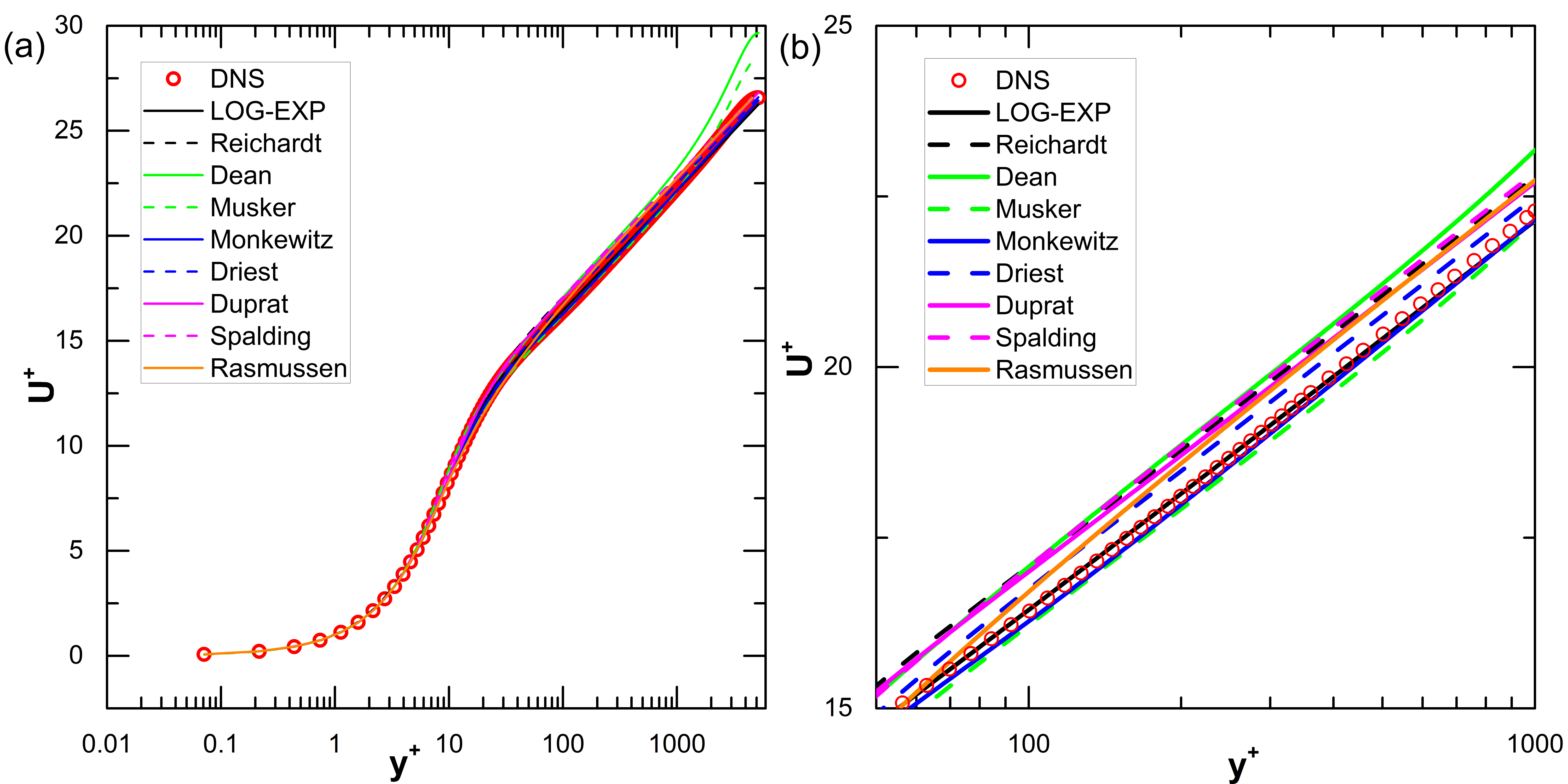
Figure 2: (a) Comparison of the velocity profiles predicted by the LOG-EXP formula and others with that from DNS for the turbulent channel flow at Reynolds numbers $Re_{\tau}=5200$ (b) Zoomed-in plot of (a) for $50\leq y^{+}\leq 1000$.

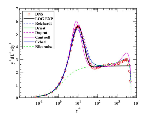
Figure 3: Comparison of $y^{+}dU^{+}/dy^{+}$ predicted by the LOG-EXP formula and others with that from DNS for the turbulent channel flow at Reynolds numbers $Re_{\tau}=5200$.

In Figure 4 and Figure 5, we compare predictions from the proposed LOG-EXP formula with the DNS data Lee and Moser (2014) for different Reynolds numbers. Although minor differences are observed for the low Reynolds number case with $Re_{\tau}=180$, an overall good agreement is observed for both the velocity profile and the first derivative of $dU^{+}/dy^{+}$ for the proposed LOG-EXP formula.

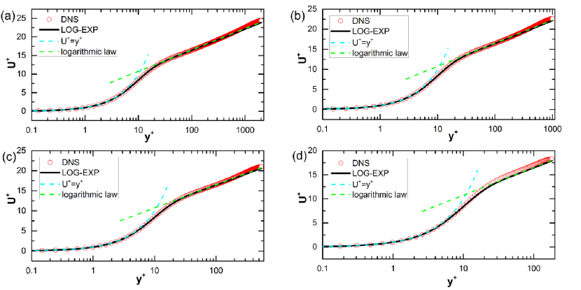
Figure 4: Comparison of the velocity profiles predicted by the LOG-EXP formula with those from DNS for the turbulent channel flow with different Reynolds numbers for (a) $Re_{\tau}=2000$, (b) $Re_{\tau}=1000$, (c) $Re_{\tau}=550$, and (d) $Re_{\tau}=180$.

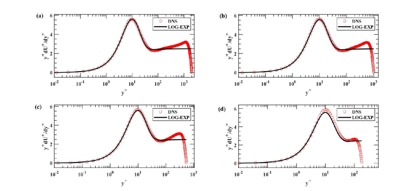
Figure 5: Comparison of $y^{+}dU^{+}/dy^{+}$ predicted by the LOG-EXP formula with those from DNS for the turbulent channel flow with different Reynolds numbers for (a) $Re_{\tau}=2000$, (b) $Re_{\tau}=1000$, (c) $Re_{\tau}=550$, and (d) $Re_{\tau}=180$.

To qualitatively evaluate the proposed LOG-EXP formula, we calculate the maximum absolute error of the velocity, which is defined by

$$e_{\text{max, }U^{+}}=\mathop{\max}_{0\leq\frac{y}{\delta}\leq 0.3}\frac{|U_{F}^{+}-U_{DNS}^{+}|}{\langle\left|U_{DNS}^{+}\right|\rangle},$$ (13)

where $U_{DNS}^{+}$ , $~{}U_{F}^{+}$ and $\langle U_{DNS}^{+}\rangle$ are the velocity of the DNS data, the velocity calculated by the single formula and the mean of $U_{DNS}^{+}$ averaged over $0.0\leq{y}/{\delta}\leq 0.3$, and the maximum absolute error of $dU^{+}/dy^{+}$ , which is defined by

$$e_{\text{max,}dU^{+}/dy^{+}}=\mathop{\max}_{0\leq\frac{y}{\delta}\leq 0.3}\frac{\left|\left(\frac{dU^{+}}{dy^{+}}\right)_{F}—\left(\frac{dU^{+}}{dy^{+}}\right)_{DNS}\right|}{\left\langle\left|\left(\frac{dU^{+}}{dy^{+}}\right)_{DNS}\right|\right\rangle},$$ (14)

where $\left(dU^{+}/dy^{+}\right)_{DNS}$ , $\left(dU^{+}/dy^{+}\right)_{F}$ and $\langle\left(dU^{+}/dy^{+}\right)_{DNS}\rangle$ are the first derivative of the velocity of the DNS data, the first derivative of the velocity calculated from single formula and the mean value of $\left(dU^{+}/dy^{+}\right)_{DNS}$ averaged over $0.0\leq{y}/{\delta}\leq 0.3$, respectively.

In Figure 6, we plot the errors of the velocity predicted by different formulae for different Reynolds numbers. As seen in Figure 6(a), the errors of the LOG-EXP predictions, which are less than 0.1, are lower than the other formulae except for the very low Reynolds number case. Figure 6(b) and (c) show the vertical location $y_{e_{\text{max, }U^{+}}}$ where the $e_{\text{max, }U^{+}}$ occurs for different normalization, i.e., the viscous length scale $\delta_{v}$ and the channel half-height $\delta$, respectively. It is observed that $y_{e_{\text{max, }U^{+}}}$ increases with the increase of the Reynolds number when normalized using $\delta_{v}$, while remains nearly constant for $y_{e_{\text{max, }U^{+}}}$ when normalized using $\delta$ for the proposed LOG-EXP formula,

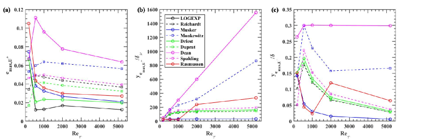
Figure 6: (a) The maximum absolute error $e_{\text{max, }U^{+}}$ of the velocity predicted by different formulae compared with DNS data for different Reynolds numbers; (b) The vertical location in wall units $y_{e_{\text{max, }U^{+}}}/\delta_{v}$ where the maximum absolute error occurs; (c) The vertical location normalized by the half-height of channel $y_{e_{\text{max, }U^{+}}}/\delta$ where the maximum absolute error occurs.

In Figure 7, the errors of the velocity derivatives predicted by different formulae are examined for different Reynolds numbers. As seen in Figure 7(a), the errors of the LOG-EXP predictions are lower than others, which increase via Reynolds number. Figure 7 (b) and (c) show the locations where the $e_{\text{max, }dU^{+}/dy^{+}}$ occurs, which are normalized by the length scales $\delta_{v}$ and $\delta$, respectively. As seen, the $y_{e_{\text{max, }dU^{+}dy^{+}}}$ for velocity derivative is close to or within the viscous sublayer for different Reynolds numbers.

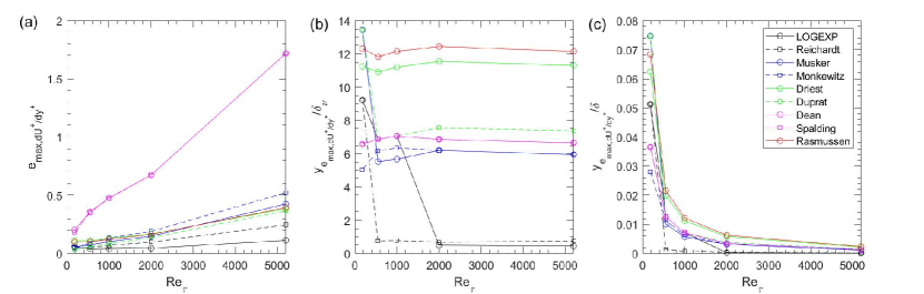
Figure 7: Same as Figure 6 but for $e_{\text{max, }dU^{+}/dy^{+}}$ and $y_{e_{\text{max, }dU^{+}dy^{+}}}$.

We further apply the proposed LOG-EXP formula to different types of canonical flows. Figure 8 shows the semi-logarithmic plots of mean velocity profiles in the circular pipe flow Laufer (1953); Lindgren and Chao (1969) and the turbulent boundary layer on a flat plate Charnay, Comte-Bellot, and Mathieu (1972). An overall good agreement between the LOG-EXP formula and the experimental data is observed in the near wall region.

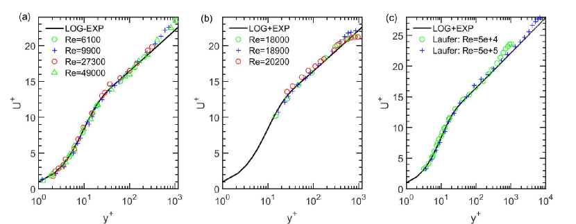
Figure 8: Comparison of the velocity profiles predicted by the LOG-EXP formula with the experimental data from (a) Lindgren and Chao Lindgren and Chao (1969),(b) Charnay et al. Charnay, Comte-Bellot, and Mathieu (1972), (c) Laufer Laufer (1953) for (a,c) the circular pipe flow and (b) the turbulent boundary layer on a flat plate.

IV Application of the LOG-EXP formula to WMLES

In this section, we apply the LOG-EXP formula to WMLES. In WMLES, the wall shear stress at the wall is often employed as approximate boundary conditions for outer flow simulations. However, the wall shear stress cannot be determined explicitly using the LOG-EXP formula. To address this issue, we employ the feedforward neural network (FNN) to construct an explicit LOG-EXP model for explicitly computing the wall shear stress (details on the model training and a priori test can be found in the appendix Appendix A: A neural network model for explicitly computing wall shear stress. The explicit LOG-EXP model is then applied in WMLES and tested using turbulent channel flows at different Reynolds numbers.

The explicit LOG-EXP model is implemented in the large-eddy simulation module of the Virtual Flow Simulator (VFS-Wind) code  Yang et al. (2015); Yang and Sotiropoulos (2018). The governing equations are the incompressible Navier-Stokes equations, which are discretized spatially using the second-order central differencing scheme, and advanced in time using a second-order fractional step method. The subgrid-scale stress is modeled using the dynamic procedure Germano et al. (1991). In the implementation of the LOG-EXP wall model, the wall-tangential component of the velocity and wall-normal distance as the second off-wall grid nodes are employed as inputs for the LOG-EXP model, with computed wall shear stresses employed as boundary conditions for the outer flow simulation. For the wall-normal component of the velocity, a no-slip boundary condition is employed.

Two cases with different Reynolds numbers are considered, i.e., the Reynolds number defined using the friction velocity $Re_{\tau}=1000$, $5200$. For both cases, the computational domain is $L_{x}\times L_{y}\times L_{z}=7.0m\times 2.0m\times 3.5m$ in the streamwise, vertical and spanwise directions, respectively, with the corresponding numbers of grid nodes $N_{x}\times N_{y}\times N_{z}=33\times 33\times 33$, which are uniformly distributed in all three directions.

We compare the predictions from WMLES with the LOG-EXP model with the DNS results Graham et al. (2016) and those from the Werner-Wengle (WW) model Werner and Wengle (1993). It is shown in Figure 9 (a) that the mean velocity profiles predicted by the WW model and the LOG-EXP model agree well with the DNS profile. For the primary Reynolds shear stress ${\left<u^{\prime}v^{\prime}\right>}^{+}$, figure 9 (b) shows that the WW model somewhat overestimates the magnitude of ${\left<u^{\prime}v^{\prime}\right>}^{+}$ for $200<y^{+}<800$, which, on the other hand, is accurately predicted by the LOG-EXP model. The comparisons of the normal Reynolds stresses are shown in Figure 9 (c, d). It is observed that both wall models overpredict the streamwise component of the normal Reynolds stress ${\left<u^{\prime}u^{\prime}\right>}^{+}$, while underpredict the wall-normal component ${\left<v^{\prime}v^{\prime}\right>}^{+}$. Comparisons for the case with $Re_{\tau}=5200$ are shown in Figure 10, with similar observations as for the case with $Re_{\tau}=1000$.

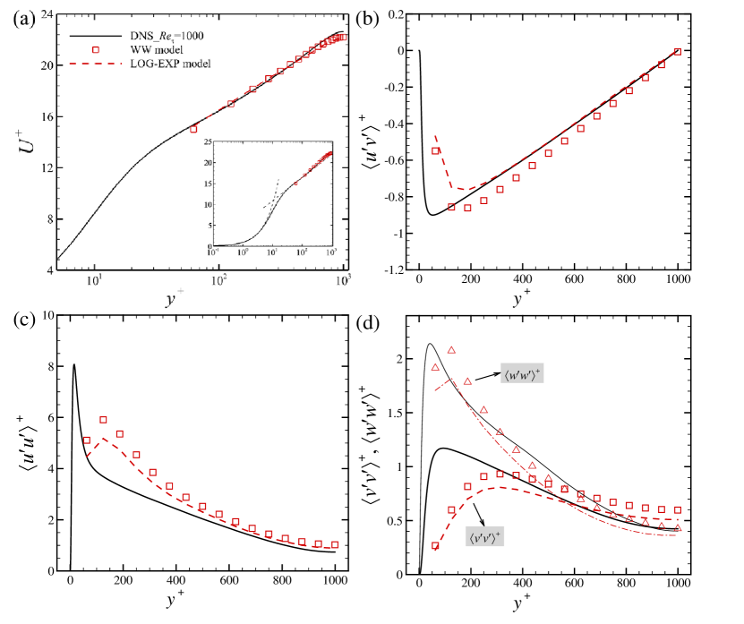
Figure 9: Comparison of predictions from the WMLES with the LOG-EXP model with DNS and those from the WW model for (a) the mean streamwise velocity, (b) the primary Reynolds shear stress ${\left<u^{\prime}v^{\prime}\right>}^{+}$, and (c, d) the normal Reynolds stresses ${\left<u^{\prime}u^{\prime}\right>}^{+}$, ${\left<v^{\prime}v^{\prime}\right>}^{+}$ and ${\left<w^{\prime}w^{\prime}\right>}^{+}$, respectively.

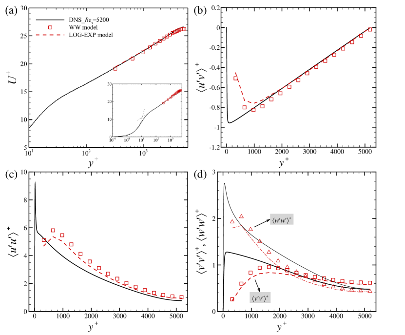
Figure 10: The same as figure  9 but for $Re_{\tau}=5200$.

V Conclusions

In this work, we proposed a new single formula for the law of the wall, which is dubbed as the LOG-EXP formula. It is derived based on the decomposition of the velocity derivative into a term satisfying the boundary conditions of the velocity derivative at the wall and in the logarithmic region, and two exponential terms accounting for the increase of turbulence as approaching the buffer layer and the viscous damping effect in the near-wall region, respectively. The derived LOG-EXP formula, which is composed of a logarithmic term and two exponential terms, works for the whole inner layer region and gives continuous predictions of both velocity and velocity derivative. Its capability is evaluated using DNS data of turbulent channel flows and some other canonical wall-bounded turbulent flows at different Reynolds numbers. Good agreements are obtained for all the considered cases.

The proposed LOG-EXP formula is then applied to WMLES. To avoid the cost of solving the LOG-EXP expression for the friction velocity, an explicit LOG-EXP model is developed using the feedforward neural network for computing wall shear stress for WMLES. The WMLES with the LOG-EXP model is evaluated using the DNS data of turbulent channel flows. An overall good agreement is obtained for both mean streamwise velocity and the Reynolds stresses.

Data availability

The data that support the findings of this study are available from the corresponding author upon reasonable request.

Appendix A: A neural network model for explicitly computing wall shear stress

In this appendix, we describe the procedure for constructing a neural network model for explicitly computing the wall shear stress using the wall-normal distance and the streamwise velocity, which can be used directly in WMLES without the need to solve the implicit LOG-EXP formula. As shown in Figure 11, a multi-hidden-layer feedforward neural network is employed for the construction of the explicit model, which contains an input layer, multi hidden layers and an output layer. Each layer has a number of neurons, which are computational units that take weighted sums of the inputs to an activation function and calculate the output. Then the outputs of each layer are fed forward as inputs to the next layer. The training goal of the neural network is to find the optimal weight and bias coefficients to minimize the loss of the neural network. More details about the neural network can be found in the reference Goodfellow et al. (2016).

The structure of the neural network employed in this work is shown in Tabel 4. The activation function used in this paper is the hyperbolic tangent function (tanh), which is defined as follows:

$$f(x)=\frac{e^{x}-e^{-x}}{e^{x}+e^{-x}}.$$ (15)

The input and output data are normalized using the Min-Max scaling,

$$x^{*}=\frac{x-x_{min}}{x_{max}-x_{min}}.$$ (16)

The loss function of the neural network is set as the mean square error (MSE), which is defined as follows:

$$L_{FNN}=\frac{1}{N_{s}}\sum_{i=1}^{N_{s}}\left(y_{i}-y_{i}^{*}\right)^{2},$$ (17)

where $N_{s}$ is the number of training samples, $y_{i}$ and $y_{i}^{*}$ are the FNN output and the labeled output from the training data, respectively. Besides, the error back-propagating (BP) scheme Rumelhart, Hinton, and Williams (1986) and the Adam optimizer Kingma and Ba (2014) are implemented with Keras Chollet (2018) to train the FNN model.

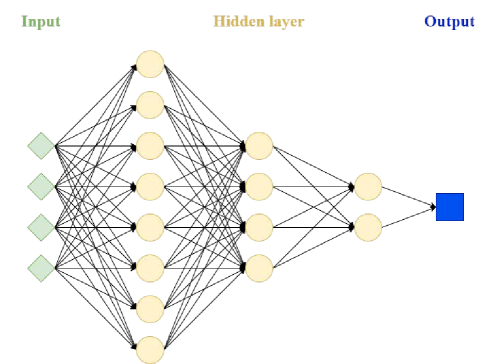
Figure 11: Schematic diagram of the feedforward neural network (FNN) with multi hidden layers.

The training data is obtained by solving the Eq. (3) about the friction velocity $u_{\tau}$ within the wall-normal distance in the range of $10^{2}<y/\nu<10^{5}$ and the streamwise velocity in the range of $0<U<1$. Data in $y^{+}<10$ are precluded because no wall model would be needed when the small scales are also resolved. Data above $y/\delta=0.1$ are not included for training because the flow away from the wall is usually resolved by LES grids. Therefore, we have $10/u_{\tau}<y/\nu<0.1Re_{\tau}/u_{\tau}$. For comparison purposes, we assume $u_{\tau}{\approx}0.05$ and $0<U<1$, which are the same as the DNS data. Then we get the approximate range of $y/\nu$. 501 points are selected evenly in the streamwise velocity range and 201 points are selected evenly in two adjacent orders of magnitude of $y/\nu$, so that the training data contains about 501 × 603 input-output pairs. The neural network is trained to predict the friction velocity for given velocity and wall-normal distance. The inputs for training the neural network, which are defined based on the expression of the LOG-EXP formula as shown in Eq. 3, are shown in Table  4.

Figure 12 (a) shows the friction velocity predicted by the FNN model, as a function of the streamwise velocity and the wall-normal distance divided by the kinematic viscosity. As seen in Figure 12 (b), the relative error of the friction velocity, which is define by

$${u_{\tau}}_{RE}=\frac{|u_{\tau}-{u_{\tau}}_{FNN}|}{u_{\tau}},$$ (18)

where $u_{\tau}$ and ${u_{\tau}}_{FNN}$ are calculated by Eq. 3 and FNN, respectively, is smaller than $0.5\%$ for most cases. And the relative error of the velocity in wall units obtained by FNN is smaller than $1\%$, except for the case when the streamwise velocity is very small. Then we test the FNN model using the DNS data of turbulent channel flow with $Re_{\tau}=1000$ Graham et al. (2016). As seen in Figure 13, the predictions from the FNN model fit well with the DNS data for different wall-normal distannces.

NN	AF	HL size	Input	Output
FNN	tanh	( 8 ,4 ,2 )	$\frac{1}{\kappa}ln(1+\frac{{\kappa}yU}{\nu}),A(1-e^{-\frac{yU}{{\nu}B}}),C(1-e^{-\frac{yU}{{\nu}D}}),\sqrt{\frac{yU}{\nu}}$	$\frac{U}{u_{\tau}}$

Table 4: Details of the neural networks. Here NN denotes neural network, AF activation function and HL hidden layer. The tabulated hidden layer size contains the number of neurons within each hidden layer.

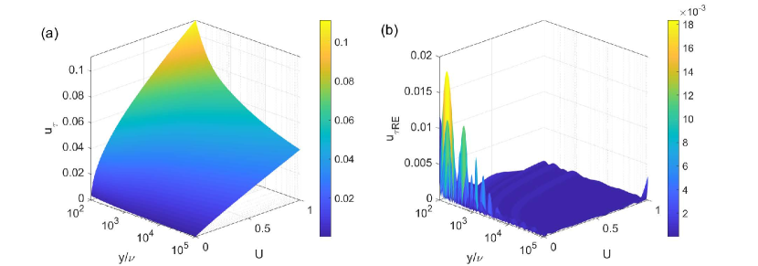
Figure 12: Test of the FNN model using the data from the LOG-EXP formula for (a) the friction velocity and (b) relative error of the friction velocity predicted by FNN.

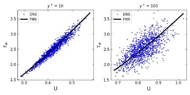
Figure 13: Test of the FNN model using the DNS data of turbulence channel flow at $Re_{\tau}=1000$ for (a) Wall shear stress as a function of the off-wall velocity at $y^{+}\approx 10$ and (b) Wall shear stress as a function of the off-wall velocity at $y^{+}\approx 100$.

References

References

- Pope (2001) S. B. Pope, Turbulent flows (Cambridge University Press, Cambridge, 2001).
- Davidson (2015) P. A. Davidson, Turbulence: an introduction for scientists and engineers (Oxford university press, 2015).
- Prandtl (1910) L. Prandtl, “Eine beziehung zwischen warmeaustausch and stromungswiderstand der flussigkeiten,” Phys. Z. 11, 1072–1078 (1910).
- Taylor (1916) G. I. Taylor, “Conditions at the surface of a hot body exposed to the wind,” Rep. Memo. of the British Advisory Committee for Aeronautics 272, 423–429 (1916).
- Kármán (1939) v. Kármán, “The analogy between fluid friction and heat transfer,” Transactions of the American Society of Mechanical Engineers 61, 705–710 (1939).
- Deissler (1954) R. G. Deissler, Analysis of turbulent heat transfer, mass transfer, and friction in smooth tubes at high Prandtl and Schmidt numbers, Vol. 1210 (National Advisory Committee for Aeronautics, 1954).
- Rannie (1956) W. D. Rannie, “Heat transfer in turbulent shear flow,” Journal of the Aeronautical Sciences 23, 485–489 (1956).
- Breuer and Rodi (1996) M. Breuer and W. Rodi, “Large eddy simulation for complex turbulent flows of practical interest,” in Flow simulation with high-performance computers II (Springer, 1996) pp. 258–274.
- Werner and Wengle (1993) H. Werner and H. Wengle, “Large-eddy simulation of turbulent flow over and around a cube in a plate channel,” in Turbulent shear flows 8 (Springer, 1993) pp. 155–168.
- Inagaki et al. (2002) M. Inagaki, O. Murata, T. Kondoh, and K. Abe, “Numerical prediction of fluid-resonant oscillation at low mach number,” AIAA journal 40, 1823–1829 (2002).
- Reichardt (1951) H. Reichardt, “Vollständige darstellung der turbulenten geschwindigkeitsverteilung in glatten leitungen,” ZAMM-Journal of Applied Mathematics and Mechanics/Zeitschrift für Angewandte Mathematik und Mechanik 31, 208–219 (1951).
- Spalding (1961) D. B. Spalding, “A single formula for the ”law of the wall”,” Transaction of the Asme Journal of Applied Mechanics 28, 455 (1961).
- Rasmussen (1975) M. Rasmussen, “On compressible turbulent boundary layers in the presence of favorable pressure gradients,” American Society of Mechanical Engineers (1975).
- Musker (1979) A. Musker, “Explicit expression for the smooth wall velocity distribution in a turbulent boundary layer,” AIAA Journal 17, 655–657 (1979).
- Dean (1976) R. Dean, “A single formula for the complete velocity profile in a turbulent boundary layer,” Journal of Fluids Engineering (1976).
- Monkewitz, Chauhan, and Nagib (2007) P. A. Monkewitz, K. A. Chauhan, and H. M. Nagib, “Self-consistent high-reynolds-number asymptotics for zero-pressure-gradient turbulent boundary layers,” Physics of Fluids 19, 115101 (2007).
- Van Driest (1956) E. R. Van Driest, “On turbulent flow near a wall,” Journal of the aeronautical sciences 23, 1007–1011 (1956).
- Duprat et al. (2011) C. Duprat, G. Balarac, O. Métais, P. M. Congedo, and O. Brugière, “A wall-layer model for large-eddy simulations of turbulent flows with/out pressure gradient,” Physics of Fluids 23, 015101 (2011).
- Cantwell (2019) B. J. Cantwell, “A universal velocity profile for smooth wall pipe flow,” Journal of Fluid Mechanics 878, 834–874 (2019).
- Rotta (1950) J. C. Rotta, “Das in wandnhe gültige geschwindigkeitsgesetz turbulenter strmungen,” Ingenieur-Archiv 18, 277–280 (1950).
- Anderson, Kays, and Moffat (1972) P. Anderson, W. M. Kays, and R. J. Moffat, “The turbulent boundary layer on a porous plate: an experimental study of the fluid mechanics for adverse free stream pressure gradients,” (1972).
- Purtell, Klebanoff, and Buckley (1981) L. Purtell, P. Klebanoff, and F. Buckley, “Turbulent boundary layer at low reynolds number,” The Physics of Fluids 24, 802–811 (1981).
- NICKELS and T. (2004) NICKELS and B. T., “Inner scaling for wall-bounded flows subject to large pressure gradients,” Journal of Fluid Mechanics 521, 217–239 (2004).
- Haritonidis (1989) J. H. Haritonidis, “A model for near-wall turbulence,” Physics of Fluids A Fluid Dynamics 1, 302–306 (1989).
- Yakhot, Khait, and Orszag (1993) A. Yakhot, V. D. Khait, and S. A. Orszag, “Analytic expression for the universal logarithmic velocity law,” Journal of Fluids Engineering 115 (1993).
- Nikuradse (1966) G. Nikuradse, “Laws of turbulent flow in smooth pipes,” (1966).
- Cebeci and Bradshaw (1984) T. Cebeci and P. Bradshaw, Physical and Computational Aspects of Convective Heat Transfer (Springer-Verlag, 1984).
- Lee and Moser (2014) M. Lee and R. D. Moser, “Direct numerical simulation of turbulent channel flow up to ,” arXiv preprint arXiv:1410.7809 (2014).
- Laufer (1953) J. Laufer, “The structure of turbulence in fully developed pipe flow,” National Advisory Committee for Aeronautics Report (1953).
- Charnay, Comte-Bellot, and Mathieu (1972) G. Charnay, G. Comte-Bellot, and J. Mathieu, “Development of a turbulent boundary layer on a flat plate in an external turbulent flow(effect of quasi-external isotropic turbulence on turbulent boundary layer development on flat plate),” AGARD Turbulent Shear Flows 9 p(SEE N 72-20273 11-12) (1972).
- Lindgren and Chao (1969) E. R. Lindgren and J. Chao, “Average velocity distribution of turbulent pipe flow with emphasis on the viscous sublayer,” The Physics of Fluids 12, 1364–1371 (1969).
- Yang et al. (2015) X. Yang, F. Sotiropoulos, R. J. Conzemius, J. N. Wachtler, and M. B. Strong, “Large-eddy simulation of turbulent flow past wind turbines/farms: the virtual wind simulator (VWiS),” Wind Energy 18, 2025–2045 (2015).
- Yang and Sotiropoulos (2018) X. Yang and F. Sotiropoulos, “A new class of actuator surface models for wind turbines,” Wind Energy 21, 285–302 (2018).
- Germano et al. (1991) M. Germano, U. Piomelli, P. Moin, and W. H. Cabot, “A dynamic subgrid-scale eddy viscosity model,” Physics of Fluids A: Fluid Dynamics 3, 1760–1765 (1991).
- Graham et al. (2016) J. Graham, K. Kanov, X. Yang, M. Lee, N. Malaya, C. Lalescu, R. Burns, G. Eyink, A. Szalay, R. Moser, et al., “A web services accessible database of turbulent channel flow and its use for testing a new integral wall model for les,” Journal of Turbulence 17, 181–215 (2016).
- Goodfellow et al. (2016) I. Goodfellow, Y. Bengio, A. Courville, and Y. Bengio, Deep learning, Vol. 1 (MIT press Cambridge, 2016).
- Rumelhart, Hinton, and Williams (1986) D. E. Rumelhart, G. E. Hinton, and R. J. Williams, “Learning representations by back-propagating errors,” nature 323, 533–536 (1986).
- Kingma and Ba (2014) D. P. Kingma and J. Ba, “Adam: A method for stochastic optimization,” arXiv preprint arXiv:1412.6980 (2014).
- Chollet (2018) F. Chollet, Deep learning with Python, Vol. 361 (Manning New York, 2018).