Neural Architecture Search for Image Super-Resolution Using Densely Constructed Search Space: DeCoNAS

Abstract

The recent progress of deep convolutional neural networks has enabled great success in single image super-resolution (SISR) and many other vision tasks. Their performances are also being increased by deepening the networks and developing more sophisticated network structures. However, finding an optimal structure for the given problem is a difficult task, even for human experts. For this reason, neural architecture search (NAS) methods have been introduced, which automate the procedure of constructing the structures. In this paper, we expand the NAS to the super-resolution domain and find a lightweight densely connected network named DeCoNASNet. We use a hierarchical search strategy to find the best connection with local and global features. In this process, we define a complexity-based penalty for solving image super-resolution, which can be considered a multi-objective problem. Experiments show that our DeCoNASNet outperforms the state-of-the-art lightweight super-resolution networks designed by handcraft methods and existing NAS-based design.

I Introduction

Single image super-resolution (SISR) is a task that creates a clearer high-resolution image from a single low-resolution input. It is an important technology that can be used as a pre-processing step to increase performances of various tasks such as medical image analysis [1], satellite image recognition [2], security image processing [3], etc. The SISR is an ill-posed problem because multiple HR images can be mapped to a single LR image. Hence, learning-based methods trained with many LR-HR image pairs are generally more effective than the interpolation-based [4] or reconstruction-based methods [5].

Recently, many deep neural networks for SISR have been developed [6, 7, 8, 9, 10, 11, 12, 13, 14, 15, 16], where Dong et al.’s SRCNN [6] is the first convolutional neural network (CNN) for the SISR. It consists of three convolution layers and yet outperformed conventional non-learning methods by a large margin. FSRCNN [7] and ESPCN [8] tried to reduce the computational cost of the structure. They used LR images directly as the input of their neural networks. Then, deconvolution and sub-pixel convolution layers were used for upsampling their results. VDSR [9] dramatically increased the depth of the model by residual learning and gradient clipping strategy. Lim et al. [10] further improved performance by a residual block composed of extensive features (EDSR) and multi-scale structure (MDSR). In MemNet [12], MSRN [16], and DenseSR [11], they proposed specific blocks in their models, such as memory block, multi-scale residual block or dense block. SelNet [17] used selection unit instead of conventional Relu operation. Zhang et al. proposed RDN [13], which consists of residual dense block and dense feature fusion that extract abundant information from the input. RCAN [18] applied channel attention mechanism to improve representational ability of CNNs. It is believed that most of these networks have been designed through laborious trials of human experts, by tuning a large number of network hyperparameters such as operation type, the number of channels, connection, depth, etc. However, a network designed by human labor may not be optimal for the given resources.

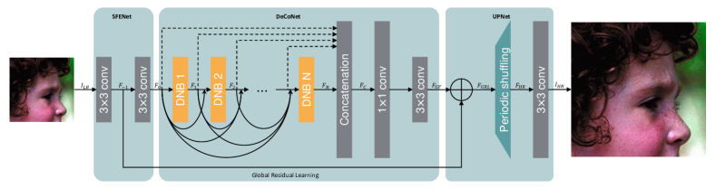
Figure 1: The architecture of the proposed DeCoNASNet system.

In the case of image classification research fields, neural architecture search (NAS) methods have been proposed [19, 20, 21, 22, 23, 24, 25, 26], which automatically find an optimal network to alleviate human labors [19, 20, 21, 22, 23, 24, 25, 26]. As a pioneering study, Zoph et al. [19] proposed a controller network that generates a child network structure based on reinforcement learning (RL). The NAS trained the controller network by REINFORCE [27], which is a kind of policy gradient algorithm. But, this method took a tremendous amount of time to evaluate the candidate models because they trained the models from scratch. To reduce the time it takes to measure the accuracy, Liu et al. [20] proposed the PNAS, which used the sequential model-based optimization (SMBO) and learned a surrogate model to predict its performance directly. Also, ENAS [21] reduced the evaluation time by about a thousand times, by applying a weight sharing scheme. The ENAS constructed a large graph and regarded each model as a sub-graph of the main graph. In this way, child networks can share their parameters while being trained separately.

Another branch of NAS algorithms is the evolutionary-based methods [22, 23, 24], which pick a population of neural networks randomly. Then, they encode the network structures as binary sequences and apply genetic modifications such as mutation and crossover to find better models. Additionally, NSGA-Net [23] used Bayesian optimization to get an advantage from its search history. Real et al. [24] introduced Amoeba-Net, which use an aging evolution algorithm to discard the earliest trained network. DARTS [25] and NAO [26] are also promising architectures that are approached differently from RL and evolutionary-based algorithm. DARTS optimized all parameters and connections in the neural architecture jointly with a continuous relaxation of the search space. NAO proposed a learnable embedding space of architectures and found the best model from it.

Recently, some researchers expanded the NAS to other domains such as object detection [28] (Auto-deeplab) and image SR [29] (MoreMNAS), [30] (FALSR). Specifically, they used a reinforced evolution algorithm and solved the image SR task as a multi-objective problem. However, these reinforced evolution algorithms need more than 1 GPU month to find optimal architectures. Furthermore, FALSR evaluated the network approximately because they did not use a complete training strategy.

To overcome these drawbacks, we take the idea of ENAS [21] as our baseline search framework. The ENAS consists of a controller and child networks, where the controller is composed of LSTM blocks to generate a child network sequence. We also use the REINFORCE [27] algorithm to train the controller in the direction of increasing PSNR of the SR results. As in the original ENAS for the classification problems, child networks share their parameters during the training and evaluation. In addition, we propose a complexity-based penalty to reduce the rewards for the networks that need a large number of parameters. We exclude redundant hierarchical information by predicting connections for local and global feature fusion through the controller.

SR is a type of regression that generally needs a deeper and more complex network than classification. Hence, in this paper, we search for a new SR architecture on the densely constructed search space. Specifically, we propose a Densely Connected Neural Architecture Search (DeCoNAS) method, which attempts to find optimal connections on the baseline of residual dense network (RDN) [13]. The proposed DeCoNAS search space consists of mix nodes for densely connected network blocks (DNB), local feature fusion, and global feature fusion. In addition to the convolution layer with $3\times 3$ filters in the baseline network, dilated convolution [31] and depth separable convolution [32] are included in the search space for better performance. Experiments show that our DeCoNASNet performs better than human-crafted networks and the existing NAS-based SR network [29, 30]

Our main contributions are summarized as follows:

I-1 A New NAS-Based SR

We propose a new NAS-based SR network design, named DeCoNAS, which searches for networks with higher performance by combining hierarchical and local information efficiently.

I-2 Complexity-Based Penalty

We design a complexity-based penalty and add it to the reward of the REINFORCE algorithm, which enables us to search for an efficient network that has high performance and fewer parameters.

I-3 Feature Fusion Layer Search

We also search for efficient feature fusion method. Instead of connecting all the global/local feature fusion layers, we design the connection to be predicted through the controller, which removes redundant hierarchical information and hence reduce network complexity.

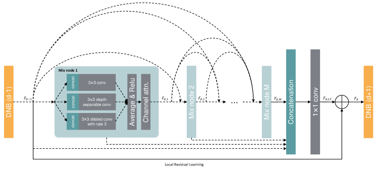
Figure 2: Detailed structure of the densely connected network blocks (DNB).

II Proposed Method

As a typical RL framework, the proposed architecture consists of two parts: a child network (denoted as DeCoNASNet) for reward measurement and a controller for network structure generation. Following ENAS [21], we try to save time by using parameter sharing when training a child network. Also, we regard the SR as a multi-objective task. That is, we design a complexity-based penalty to consider not only the PSNR but also the parameter complexity of the network for calculating the reward.

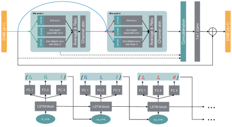
(a)

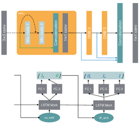
(b)

Figure 3: The example structure of our Controller and DeCoNASNet structure with 2 mix nodes ($M=2$) and 3 DNBs ($N=3$). (a) is the example for mix nodes, and (b) is the example for feature fusion layers.

We use a two-layer LSTM network in our controller to generate the DeCoNASNet structure. Supposing that the child network c consists of $N$ blocks, $M$ mix nodes, and $K$ mix node operations, the controller sequence $\textbf{S}_{\textbf{c}}$ for c is

$$\begin{split}\textbf{S}_{\textbf{c}}&=\{\textbf{S}_{M},\textbf{S}_{F}\},\\ \textbf{S}_{M}&=\{S_{i,j}^{k}\},0<i\leq M,0\leq j<i,0\leq k<K,\\ \textbf{S}_{F}&=\{{S_{l}}^{0}:{S_{l}}^{M-1},{S_{g}}^{0}:{S_{g}}^{N-1}\},\end{split}$$ (1)

where $\textbf{S}_{M}$ is the sequence for mix node configuration, and $\textbf{S}_{F}$ is the sequence for the feature fusion layer. $\textbf{S}_{F}$ consists of two sequences, $\textbf{S}_{l}$ and $\textbf{S}_{g}$, which denote the sequence for local feature fusion and global feature fusion, respectively.

II-A Overall structure of DeCoNASNet

DeCoNASNet consists of three parts as shown in Fig. 1, inspired by the RDN [13] architecture: shallow feature extractor network (SFENet), densely connected network (DeCoNet), and UPNet. The output of SFENet can be represented as

$$F_{0}=H_{SFE2}(H_{SFE1}(I_{LR})),$$ (2)

where $H(\cdot)$ denotes the convolution operation. SFENet converts the input image $I_{LR}$ into a shallow feature $F_{0}$, which is used as the input to the DeCoNet. Then, the output of the $d$-th DNB in DeCoNet, denoted by $F_{d}$ is expressed as

$$F_{d}=H_{DNB,d}(H_{1}(concat(F_{0},F_{1},\dots,F_{d-1}))),$$ (3)

where $H_{DNB}(\cdot)$ denotes the DNB operation and $H_{1}(\cdot)$ is $1\times 1$ convolution to match the input channels of DNBs. We will explain the operation $H_{DNB}(\cdot)$ in the next subsection. We omit $H_{1}(\cdot)$ and concatenation operation in Fig. 1 for simplicity. The global feature fusion layer follows after the $N$-th DNB to combine the information of the features of DNB. The output of the global feature fusion layer, denoted by $F_{GF}$ is described as

$$\begin{split}F_{GF}&=H_{GFF}(F_{C}),\\ F_{C}&=concat({S_{g}}^{0}\cdot F_{0},\dots,{S_{g}}^{N-1}\cdot F_{N-1},F_{N}),\end{split}$$ (4)

where $H_{GFF}(\cdot)$ denotes the $1\times 1$ convolution and $3\times 3$ convolution operation, ${S_{g}}^{i}$ denotes the output global feature fusion sequence of controller, and $concat(\cdot)$ denotes the concatenation of features. We omit $F_{i}$ when concatenating features if ${S_{g}}^{i}$ is zero. All of the ${S_{g}}^{i}$ equal to one if we do not use the feature fusion search strategy. The UPNet combines the output of DeCoNet and $F_{-1}$, which is the shallow feature from the SFENet. We use periodic shuffling operation and applied $3\times 3$ convolution as in ESPCN [8], to convert LR features to high-resolution images. We fix the SFENet and the UPNet, while we search for the DeCoNet. In all of our figures, we use dashed arrows to depict that the connection is to be searched.

II-B Constructing the DNB

We apply the same operation $H_{DNB}(\cdot)$ through all the DNBs. Each DNB consists of M mix nodes as shown in Fig. 2, where there are three element candidates in the mix node:

• $3\times 3$ 2D convolution,

• $3\times 3$ depth separable convolution,

• $3\times 3$ dilated convolution with rate $3$.

Also, $F_{d,m}$ over the arrow is the output of the $m$-th mix node in the $d$-th DNB with K candidate mix node operations, which are obtained as

$$F_{d,m}=\begin{cases}F_{d,m-1},&\mbox{if }\textbf{S}_{m,0:m-1}^{0:K-1}=\textbf{0}\\ CA(Relu(average(\textbf{F}_{inter}))),&\mbox{else }\end{cases}$$ (5)

where

$$\begin{split}\textbf{F}_{inter}&={F_{d,m}^{0:K-1}},\\ F_{d,m}^{i}&=H_{i}(concat(S_{m,0}^{i}\cdot F_{d,0},\dots,S_{m,m-1}^{i}\cdot F_{d,m-1}))\end{split}$$ (6)

where $H_{i}(\cdot)$ denotes the $i$-th operation in $K$ operations, and $\textbf{S}_{m,0:m-1}^{0:K-1}$ is the sequence for the $m$-th mix node configuration. Same as the Eq. (4), we omit $F_{d,m}^{i}$ or $F_{d,m}$ if $\textbf{S}_{m,0:m-1}^{i}=\textbf{0}$ or $S_{m,j}^{i}=0$ in Eq. (6). $CA(\cdot)$ in Eq. (5) denotes channel attention network used in RCAN [18].

II-C Constructing controller for the DeCoNASNet

II-C1 Controller output of the mix node

We need $i\times K$ sequences to create the $i$-th mix node. Hence, our controller is composed of $\sum_{i=1}^{M}i=\frac{M(M+1)}{2}$ LSTM blocks, and $K$ fully connected layers are connected to each LSTM block. For example, As shown in Fig. 3(a), we use 3 LSTM blocks and 9 outputs to create the connections for two mix nodes.

II-C2 Controller output of the feature fusion layer

There are two LSTM blocks for feature fusion layer search. These blocks are connected to the last LSTM block for mix node, in order to include the information about the mix node structure. Like the mix node, we connect $N$ and $M$ fully connected layers to two LSTM blocks, respectively. The output from each LSTM block denotes the connection between the mix node and the feature fusion layer. Fig. 3(b) shows an example connection of local/global feature fusion layer.

II-D Training DeCoNAS and complexity-based penalty

Following ENAS [21], the DeCoNAS has two learnable parameters. The parameter of the controller is $\boldsymbol{\theta}$, and the parameter of the child network is w. To learn $\boldsymbol{\theta}$ and w alternately, we use a two-step learning strategy. In the first step, we train w using training data. We use an RL scheme to train $\boldsymbol{\theta}$, with the reward signal consisting of peak signal to noise ratio (PSNR) and complexity-based penalty.

II-D1 Training child network

As the first step to training DeCoNAS, we need to learn w, which is the parameter of the child network, c. This problem is defined as

$$\min_{\textbf{w}}\operatorname*{\mathbb{E}}_{\textbf{c}\sim\pi(\textbf{c};\boldsymbol{\theta})}[L(\textbf{c};\textbf{w})].$$ (7)

To optimize w, we fix the controller’s policy $\pi(\textbf{c};\boldsymbol{\theta})$ and use Adam optimizer [33]. In this case, we use the L1 loss for $L(\textbf{c};\textbf{w})$, calculated on training data and model c generated by $\pi(\textbf{c};\boldsymbol{\theta})$. Gradient of $\operatorname*{\mathbb{E}}_{\textbf{c}\sim\pi(\textbf{c};\boldsymbol{\theta})}[L(\textbf{c};\textbf{w})]$ is calculated by Monte Carlo estimate

$$\bigtriangledown_{\textbf{w}}\operatorname*{\mathbb{E}}_{\textbf{c}\sim\pi(\textbf{c};\boldsymbol{\theta})}[L(\textbf{c};\textbf{w})]\approx\frac{1}{M}\sum_{i=1}^{M}\bigtriangledown_{\textbf{w}}L(\textbf{c}_{i};\textbf{w}),$$ (8)

where $\textbf{c}_{i}$’s are sampled by the controller’s policy $\pi(\textbf{c};\boldsymbol{\theta})$. As mentioned in ENAS [21], w can be optimized by calculating the gradient for only one model c generated by $\pi(\textbf{c};\boldsymbol{\theta})$ for each mini-batch.

II-D2 Training controller with performance reward and complexity-based penalty

In the second step, we need to train $\boldsymbol{\theta}$, which is the controller’s parameter. This problem is to maximize the expected reward as

$$\max_{\boldsymbol{\theta}}E_{P(a_{1:T};\boldsymbol{\theta})}[R],$$ (9)

where $a_{1:T}$ is the controller output for the child network c, which follows the distribution of $\pi(\textbf{c};\boldsymbol{\theta})$. We compute the gradient of the problem by using the approximation of gradients in REINFORCE [27] as

$$\bigtriangledown_{\boldsymbol{\theta}}\operatorname*{\mathbb{E}}_{P(a_{1:T};\boldsymbol{\theta})}[R]=\sum_{t=1}^{T}[\bigtriangledown_{\boldsymbol{\theta}}\log P(a_{t}|a_{t-1:1};\boldsymbol{\theta})(R-b)]$$ (10)

where $b$ is the baseline for reducing the variance, which is the moving average of the reward. While ENAS used classification accuracy for $R$, we calculate it differently as

$$R=p(\textbf{c},\textbf{w})–\alpha*cb(\textbf{c}),$$ (11)

where $p(\textbf{c},\textbf{w})$ is the PSNR of model c. We calculate the PSNR using the validation set rather than the training set to prevent overfitting. Also, $cb(\textbf{c})$ is the complexity-based penalty, calculated as

$$cb(\textbf{c})=\frac{n_{m}}{n_{cm}},$$ (12)

where $n_{m}$ denotes the number of parameters in the generated model c and $n_{cm}$ indicates the number of parameters in the most complex model in the search space. We also multiply $\alpha$ by $cb(\textbf{c})$, allowing the user to set a trade-off between the performance and model complexity. Finally, we use Adam optimizer [33] to maximize the reward.

III Experimental results

III-A Settings

III-A1 Datasets and metrics

We use DIV2K dataset [34] for the training, which has been widely used for training image restoration networks. The DIV2K contains 800 training images, 100 validation images, and 100 test images. We use all images in the training set to train our DeCoNASNet, and use all of the validation images when calculating the reward and training the controller. Experiments are conducted on four benchmark datasets, Set5 [35], Set14 [36], B100 [37], and Urban100 [38], where we compute PSNR and SSIM [39] on the Y channel.

III-A2 Implemenation details

Our proposed DeCoNASNet has 4 DNBs, and each DNB has 4 mix nodes. The output channel of SFENet and DNB are both 64. The $3\times 3$ convolution layer in UPNet also has 64 output channels, and we conduct periodic shuffling on the feature maps. The final convolution layer has $3\times 3$ filters and three output channels to restore the high-resolution images.

The LSTM block in the controller is made of two stacked LSTM layers with 64 hidden states. Fully connected layers for one operation in each LSTM block are sharing their parameters. We tie the LSTM outputs with word embeddings [40] to make the input of the next LSTM block.

III-A3 Training setting

In the search phase, we need to train controller and DeCoNASNet together. We use variance scaled initialization [41] with 0.02 scaling value for DeCoNASNet parameter w and controller parameter $\boldsymbol{\theta}$. To train the controller, we apply 100 iterations for one epoch, and the learning rate is fixed to $3\times 10^{-4}$.

TABLE I: Performance comparison between search settings.

Search setting		CB0_FF0	CB0_FF1	CB1_FF0	CB1_FF1
Best	PSNR	35.919	35.602	35.894	35.436
	Parameters	22.9 M	25.4 M	18.0 M	25.9 M
Mean	PSNR	35.294	35.168	35.324	35.025
	Parameters	22.5 M	28.4 M	17.1 M	24.9M

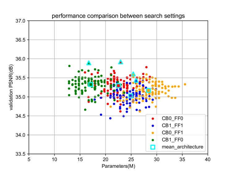
Figure 4: Scatter plot of 100 samples for each search setting.

For training the DeCoNASNet, we randomly extract 16 LR patches of size $64\times 64$ from the DIV2K training image as the input to the network. After extracting the patches, we apply horizontal flip and 90°, 180°, 270° rotations to each patch randomly for data augmentation. We conduct 1,000 backpropagation for an epoch, where Adam optimizer [33] is used for updating parameters. The learning rate is initialized to $10^{-4}$ and decreased by half for every $5\times 10^{5}$ iterations (50 epochs), and 200 epochs are conducted for the search phase. We sample 100 candidate structures by the trained controller and choose the best architecture as our DeCoNASNet structure. After choosing the best architectures, we train the DeCoNASNet for 1,000 epochs. The learning rate is initialized to $10^{-4}$ and decreases by half for every 200 epochs. The other settings are the same as the search phase.

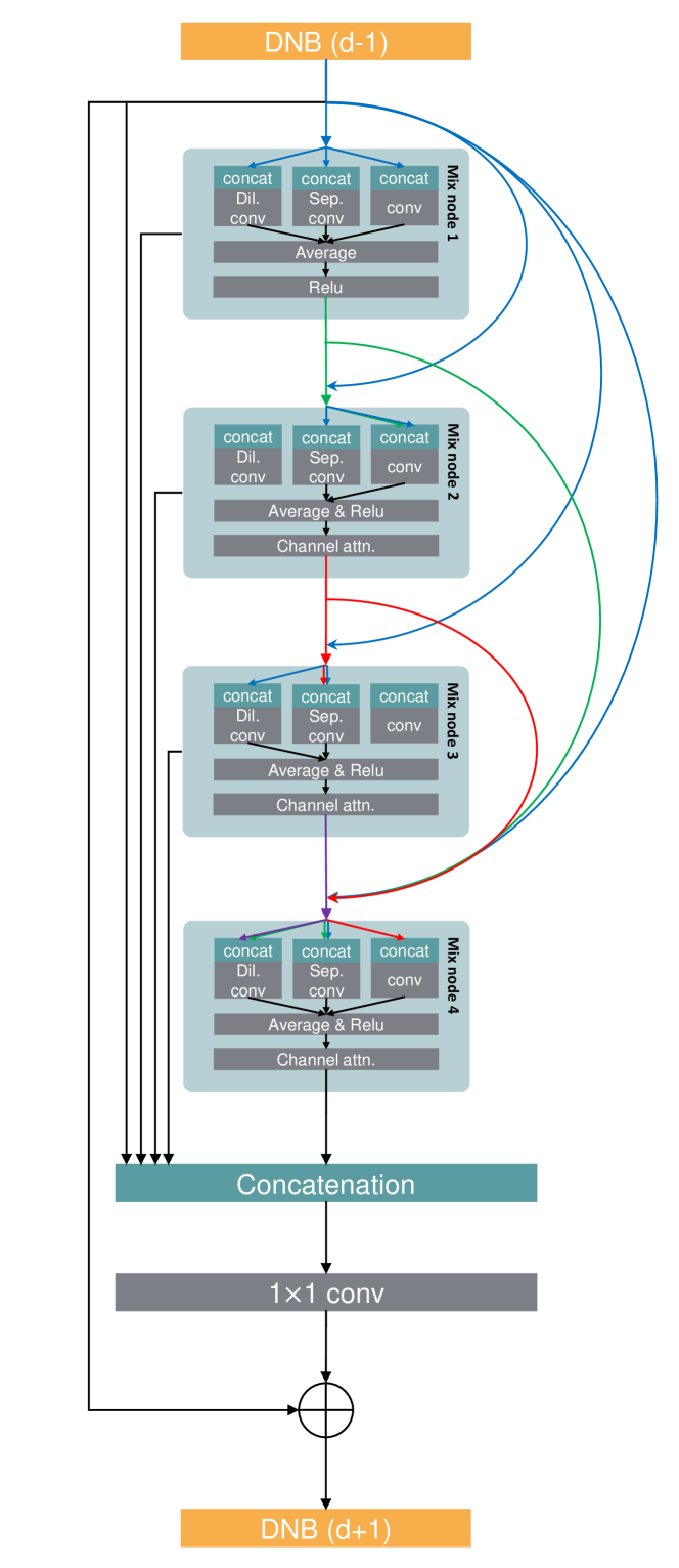
Figure 5: Our DeCoNASNet model found by controller.

TABLE II: Public benchmark test results (PSNR/SSIM) for $\times 2$ SR. The red color means the best performance and the blue means the second best. The “Design time” at the last column indicates the times taken by the NAS approaches.

Model	Params	Set 5	Set 14	B100	Uban100	Design time
Bicubic	-	33.66 / 0.9299	30.24 / 0.8688	29.56 / 0.8431	26.88 / 0.8403	-
SRCNN [6]	57K	36.66 / 0.9542	32.45 / 0.9067	31.36 / 0.8879	29.50 / 0.8946	-
VDSR [9]	665K	37.53 / 0.9587	33.03 / 0.9124	31.90 / 0.8960	30.76 / 0.9140	-
LapSRN [15]	813K	37.52 / 0.9591	33.08 / 0.9130	31.80 / 0.8950	30.41 / 0.9101	-
MemNet [12]	677K	37.78 / 0.9597	33.28 / 0.9142	32.08 / 0.8978	31.31 / 0.9195	-
SelNet [17]	970K	37.89 / 0.9598	33.61 / 0.9160	32.08 / 0.8984	- / -	-
CARN [14]	1,582K	37.76 / 0.9590	33.52 / 0.9166	32.09 / 0.8978	31.92 / 0.9256	-
MoreMNAS-A [29]	1,039K	37.63 / 0.9584	33.23 / 0.9138	31.95 / 0.8961	31.24 / 0.9187	56 GPU days
FALSR-A [30]	1,021K	37.82 / 0.9595	33.55 / 0.9168	32.12 / 0.8987	31.93 / 0.9256	24 GPU days
DeCoNASNet (ours)	1,713K	37.96 / 0.9594	33.63 / 0.9175	32.15 / 0.8986	32.03 / 0.9265	12 GPU hours

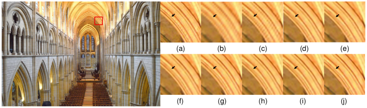
Figure 6: Qualitative comparison of the conventional methods and ours. (a) HR image, (b) bicubic LR image, (c) SRCNN [6], (d) VDSR [9], (e) LapSRN [15], (f) MemNet [12], (g) CARN [14], (h) MoreMNAS [29], (i) FALSR [30], (j) DeCoNASNet (ours).

III-B Results

III-B1 DeCoNAS search result

We use 16 DNBs ($N=16$) and 8 mix nodes in each DNB ($M=8$) to verify the effect of feature fusion strategy and complexity-based penalty. Table I and Fig. 4 show the performance of total 400 DeCoNAS structures in four settings (100 structures each). The baseline setting (denoted as FF0_CB0), which omitted the feature fusion search (FF) and complexity-based penalty (CB), shows the best performance with 23.2 M parameters. We add one of CB or FF to FF0_CB1 and FF1_CB0. From the results, we can also see that FF0_CB1 achieves almost the same performance as the baseline search strategy, with 20% less parameters, and FF1_CB0 has slightly lower performance with large parameters. Finally, we apply both strategies, resulting in FF1_CB1, which is shown to have fewer parameters than the FF1_CB0 model, but yields inferior performance than the others. Further discussions about CB and FF strategies are at the ablation study section.

We use 4 DNBs ($N=4$) and 4 mix nodes ($M=4$) in each DNB to make DeCoNASNet structure. We choose the best architecture which belongs to FF0_CB1 setting. Fig. 5 shows the DNB structure of DeCoNASNet:{7, 6, 4, 3, 0, 2, 2, 3, 4, 1}. The local/global feature fusion connections are all connected because we do not use the feature fusion search strategy. We regard three outputs of each controller LSTM block as the binary number and convert it to a decimal number for simplicity. For example, four in the sequence means {1, 0, 0} and six is {1, 1, 0}. It takes about 12 hours by 1 Titan XP GPU to search for the DeCoNASNet structure, which is far less than other NAS-based methods.

III-B2 Comparison with state-of-the-art methods

We compare our DeCoNASNet with six lightweight networks (SRCNN [6], VDSR [9], MemNet [12], LapSRN [15], SelNet [17], CARN [14]) and two NAS-based methods (MoreMNAS [29], FALSR [30]). The results are shown in Table II, where we can see that DeCoNASNet outperforms other hand-crafted lightweight models and existing NAS-based ones while using somewhat more parameters, still within 2M. The most important advantage of our method is that it finds the optimal structure within 16 hours, which is $\times 50$ faster than other NAS-based methods.

We compare the visual results of our model with the others (SRCNNN [6], VDSR [9], LapSRN [15], MemNet [12], CARN [14], MoreMNAS [29], FALSR [30]) in Fig. 6. We find that DeCoNASNet successfully restores the details in images. Specifically, DeCoNASNet and CARN restore the double curves at the black arrow, while others do not.

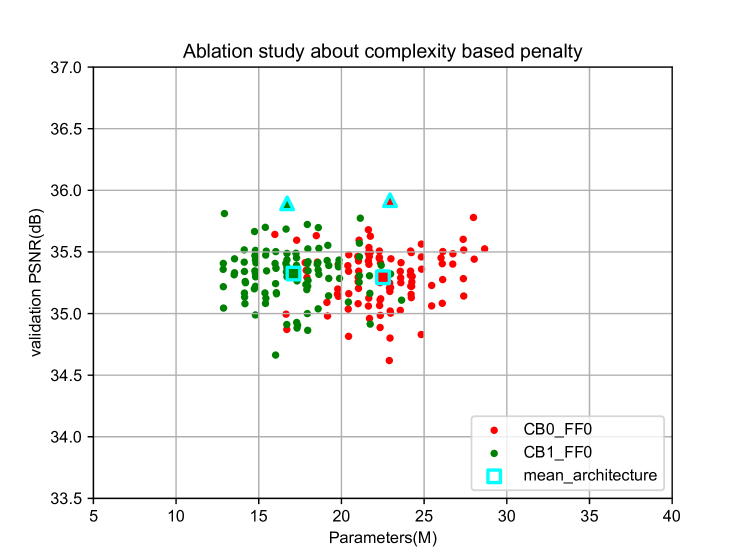
Figure 7: Ablation analysis about effect of the complexity-based penalty.

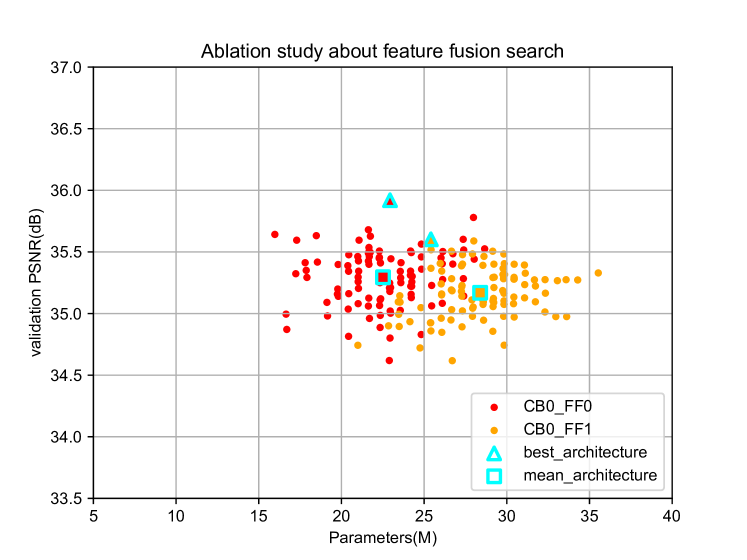
Figure 8: Ablation analysis about the feature fusion search strategy.

III-C Ablation study

Fig. 7 shows a comparison between different complexity-based penalty coefficients, $\alpha$. We conduct two experiments in the DeCoNAS search space ($N=16$, $M=8$) to analyze the effect of the complexity-based penalty. The baseline strategy is denoted as CB0_FF0, and the other strategy using CB coefficient $\alpha=2$ is described as CB1_FF0. The parameters of the searched model are decreased, but the performance difference is small when we change the CB strategy. Hence, we can validate that the complexity-based penalty efficiently controls the trade-off between the performance and the number of parameters. Users can choose $\alpha$ to find models that fit their purpose.

We also show the effect of feature fusion search (FF) strategy in Fig. 8. The red and orange dots in the figure denote CB0_FF0 and CB0_FF1, respectively. It can be seen that the FF strategy tends to find more complex models than no FF strategy. This is mainly because the controller tries to compensate for the information loss from the feature fusion layer disconnection. We can verify that the connections to the global/local feature fusion layer are more important than the connections in the mix node.

IV Conclusion

We have proposed an RL-based neural architecture search algorithm for image SR, named as DeCoNAS. It is shown that the proposed method can find a promising lightweight SR network (DeCoNASNet) within 16 hours, which is a lot faster than other NAS-based algorithms. We have also proposed a feature fusion search strategy in the proposed searching scheme, which verified the importance of global/local fusion structure for the SR. Moreover, our complexity-based penalty to the reward could reduce the network complexity, which enabled lightweight network architecture. Experiments show that the resulted DeCoNASNet yields higher performance in terms of PSNR vs. complexity among the recent handcrafted lightweight SR networks and other NAS-based ones.

References

- [1] J. S. Isaac and R. Kulkarni, “Super resolution techniques for medical image processing,” in 2015 International Conference on Technologies for Sustainable Development (ICTSD). IEEE, 2015, pp. 1–6.
- [2] Y. Luo, L. Zhou, S. Wang, and Z. Wang, “Video satellite imagery super resolution via convolutional neural networks,” IEEE Geoscience and Remote Sensing Letters, vol. 14, no. 12, pp. 2398–2402, 2017.
- [3] W. W. Zou and P. C. Yuen, “Very low resolution face recognition problem,” IEEE Transactions on image processing, vol. 21, no. 1, pp. 327–340, 2011.
- [4] L. Zhang and X. Wu, “An edge-guided image interpolation algorithm via directional filtering and data fusion,” IEEE transactions on Image Processing, vol. 15, no. 8, pp. 2226–2238, 2006.
- [5] K. Zhang, X. Gao, D. Tao, and X. Li, “Single image super-resolution with non-local means and steering kernel regression,” IEEE Transactions on Image Processing, vol. 21, no. 11, pp. 4544–4556, 2012.
- [6] C. Dong, C. C. Loy, K. He, and X. Tang, “Learning a deep convolutional network for image super-resolution,” in European conference on computer vision. Springer, 2014, pp. 184–199.
- [7] C. Dong, C. C. Loy, and X. Tang, “Accelerating the super-resolution convolutional neural network,” in European conference on computer vision. Springer, 2016, pp. 391–407.
- [8] W. Shi, J. Caballero, F. Huszár, J. Totz, A. P. Aitken, R. Bishop, D. Rueckert, and Z. Wang, “Real-time single image and video super-resolution using an efficient sub-pixel convolutional neural network,” in Proceedings of the IEEE conference on computer vision and pattern recognition, 2016, pp. 1874–1883.
- [9] J. Kim, J. Kwon Lee, and K. Mu Lee, “Accurate image super-resolution using very deep convolutional networks,” in Proceedings of the IEEE conference on computer vision and pattern recognition, 2016, pp. 1646–1654.
- [10] B. Lim, S. Son, H. Kim, S. Nah, and K. Mu Lee, “Enhanced deep residual networks for single image super-resolution,” in Proceedings of the IEEE conference on computer vision and pattern recognition workshops, 2017, pp. 136–144.
- [11] T. Tong, G. Li, X. Liu, and Q. Gao, “Image super-resolution using dense skip connections,” in Proceedings of the IEEE International Conference on Computer Vision, 2017, pp. 4799–4807.
- [12] Y. Tai, J. Yang, X. Liu, and C. Xu, “Memnet: A persistent memory network for image restoration,” in Proceedings of the IEEE international conference on computer vision, 2017, pp. 4539–4547.
- [13] Y. Zhang, Y. Tian, Y. Kong, B. Zhong, and Y. Fu, “Residual dense network for image super-resolution,” in Proceedings of the IEEE conference on computer vision and pattern recognition, 2018, pp. 2472–2481.
- [14] N. Ahn, B. Kang, and K.-A. Sohn, “Fast, accurate, and lightweight super-resolution with cascading residual network,” in Proceedings of the European Conference on Computer Vision (ECCV), 2018, pp. 252–268.
- [15] W.-S. Lai, J.-B. Huang, N. Ahuja, and M.-H. Yang, “Deep laplacian pyramid networks for fast and accurate super-resolution,” in Proceedings of the IEEE conference on computer vision and pattern recognition, 2017, pp. 624–632.
- [16] J. Li, F. Fang, K. Mei, and G. Zhang, “Multi-scale residual network for image super-resolution,” in Proceedings of the European Conference on Computer Vision (ECCV), 2018, pp. 517–532.
- [17] J.-S. Choi and M. Kim, “A deep convolutional neural network with selection units for super-resolution,” in Proceedings of the IEEE Conference on Computer Vision and Pattern Recognition Workshops, 2017, pp. 154–160.
- [18] Y. Zhang, K. Li, K. Li, L. Wang, B. Zhong, and Y. Fu, “Image super-resolution using very deep residual channel attention networks,” in Proceedings of the European Conference on Computer Vision (ECCV), 2018, pp. 286–301.
- [19] B. Zoph and Q. V. Le, “Neural architecture search with reinforcement learning,” arXiv preprint arXiv:1611.01578, 2016.
- [20] C. Liu, B. Zoph, M. Neumann, J. Shlens, W. Hua, L.-J. Li, L. Fei-Fei, A. Yuille, J. Huang, and K. Murphy, “Progressive neural architecture search,” in Proceedings of the European Conference on Computer Vision (ECCV), 2018, pp. 19–34.
- [21] H. Pham, M. Y. Guan, B. Zoph, Q. V. Le, and J. Dean, “Efficient neural architecture search via parameter sharing,” arXiv preprint arXiv:1802.03268, 2018.
- [22] L. Xie and A. Yuille, “Genetic cnn,” in Proceedings of the IEEE international conference on computer vision, 2017, pp. 1379–1388.
- [23] Z. Lu, I. Whalen, V. Boddeti, Y. Dhebar, K. Deb, E. Goodman, and W. Banzhaf, “Nsga-net: neural architecture search using multi-objective genetic algorithm,” in Proceedings of the Genetic and Evolutionary Computation Conference, 2019, pp. 419–427.
- [24] E. Real, A. Aggarwal, Y. Huang, and Q. V. Le, “Regularized evolution for image classifier architecture search,” in Proceedings of the aaai conference on artificial intelligence, vol. 33, 2019, pp. 4780–4789.
- [25] H. Liu, K. Simonyan, and Y. Yang, “Darts: Differentiable architecture search,” arXiv preprint arXiv:1806.09055, 2018.
- [26] R. Luo, F. Tian, T. Qin, E. Chen, and T.-Y. Liu, “Neural architecture optimization,” in Advances in neural information processing systems, 2018, pp. 7816–7827.
- [27] R. J. Williams, “Simple statistical gradient-following algorithms for connectionist reinforcement learning,” Machine learning, vol. 8, no. 3-4, pp. 229–256, 1992.
- [28] C. Liu, L.-C. Chen, F. Schroff, H. Adam, W. Hua, A. L. Yuille, and L. Fei-Fei, “Auto-deeplab: Hierarchical neural architecture search for semantic image segmentation,” in Proceedings of the IEEE Conference on Computer Vision and Pattern Recognition, 2019, pp. 82–92.
- [29] X. Chu, B. Zhang, R. Xu, and H. Ma, “Multi-objective reinforced evolution in mobile neural architecture search,” arXiv preprint arXiv:1901.01074, 2019.
- [30] X. Chu, B. Zhang, H. Ma, R. Xu, J. Li, and Q. Li, “Fast, accurate and lightweight super-resolution with neural architecture search,” arXiv preprint arXiv:1901.07261, 2019.
- [31] F. Yu and V. Koltun, “Multi-scale context aggregation by dilated convolutions,” arXiv preprint arXiv:1511.07122, 2015.
- [32] F. Chollet, “Xception: Deep learning with depthwise separable convolutions,” in The IEEE Conference on Computer Vision and Pattern Recognition (CVPR), July 2017.
- [33] D. P. Kingma and J. Ba, “Adam: A method for stochastic optimization,” in 3rd International Conference on Learning Representations, ICLR 2015, San Diego, CA, USA, May 7-9, 2015, Conference Track Proceedings, 2015.
- [34] R. Timofte, E. Agustsson, L. Van Gool, M.-H. Yang, and L. Zhang, “Ntire 2017 challenge on single image super-resolution: Methods and results,” in Proceedings of the IEEE conference on computer vision and pattern recognition workshops, 2017, pp. 114–125.
- [35] M. Bevilacqua, A. Roumy, C. Guillemot, and M. L. Alberi-Morel, “Low-complexity single-image super-resolution based on nonnegative neighbor embedding,” 2012.
- [36] R. Zeyde, M. Elad, and M. Protter, “On single image scale-up using sparse-representations,” in International conference on curves and surfaces. Springer, 2010, pp. 711–730.
- [37] D. Martin, C. Fowlkes, D. Tal, and J. Malik, “A database of human segmented natural images and its application to evaluating segmentation algorithms and measuring ecological statistics,” in Proceedings Eighth IEEE International Conference on Computer Vision. ICCV 2001, vol. 2. IEEE, 2001, pp. 416–423.
- [38] J.-B. Huang, A. Singh, and N. Ahuja, “Single image super-resolution from transformed self-exemplars,” in Proceedings of the IEEE conference on computer vision and pattern recognition, 2015, pp. 5197–5206.
- [39] Z. Wang, A. C. Bovik, H. R. Sheikh, and E. P. Simoncelli, “Image quality assessment: from error visibility to structural similarity,” IEEE transactions on image processing, vol. 13, no. 4, pp. 600–612, 2004.
- [40] H. Inan, K. Khosravi, and R. Socher, “Tying word vectors and word classifiers: A loss framework for language modeling,” in 4th International Conference on Learning Representations, ICLR 2016, San Juan, Puerto Rico, May 2-4, 2016, Conference Track Proceedings, 2016.
- [41] K. He, X. Zhang, S. Ren, and J. Sun, “Delving deep into rectifiers: Surpassing human-level performance on imagenet classification,” in Proceedings of the IEEE international conference on computer vision, 2015, pp. 1026–1034.