Testing the effect of resolution on gravitational fragmentation with Lagrangian hydrodynamic schemes

Abstract

To study the resolution required for simulating gravitational fragmentation with newly developed Lagrangian hydrodynamic schemes, Meshless Finite Volume method (MFV) and Meshless Finite Mass method (MFM), we have performed a number of simulations of the Jeans test and compared the results with both the expected analytic solution and results from the more standard Lagrangian approach: Smoothed Particle Hydrodynamics (SPH). We find that the different schemes converge to the analytic solution when the diameter of a fluid element is smaller than a quarter of the Jeans wavelength, $\lambda_{\mathrm{J}}$. Among the three schemes, SPH/MFV shows the fastest/slowest convergence to the analytic solution. Unlike the well-known behaviour of Eulerian schemes, none of the Lagrangian schemes investigated displays artificial fragmentation when the perturbation wavelength, $\lambda$, is shorter than $\lambda_{\mathrm{J}}$, even at low numerical resolution. For larger wavelengths ($\lambda>\lambda_{\mathrm{J}}$) the growth of the perturbation is delayed when it is not well resolved. Furthermore, with poor resolution, the fragmentation seen with the MFV scheme proceeds very differently compared to the converged solution. All these results suggest that, when unresolved, the ratio of the magnitude of hydrodynamic force to that of self-gravity at the sub-resolution scale is the largest/smallest in MFV/SPH, the reasons for which we discussed in detail. These tests are repeated to investigate the effect of kernels of higher-order than the fiducial cubic spline. Our results indicate that the standard deviation of the kernel is a more appropriate definition of the ‘size’ of a fluid element than its compact support radius.

1 Introduction

In the formation of astronomical objects, such as stars and galaxies, self-gravity plays a central role. The non-linearity of these formation processes is one of the main reasons numerical simulations remain an essential part of astrophysical research at a variety of scales. Knowing the numerical requirements to follow gravitational collapse and fragmentation correctly by any specific numerical scheme is, therefore, of utmost importance.

Truelove et al. (1997) showed, by using an Eulerian adaptive mesh refinement (AMR) finite difference method, that the cell size $d$ must satisfy the Jeans condition, $d<\lambda_{\mathrm{J}}/4$, where $\lambda_{\mathrm{J}}=(\pi c_{\mathrm{s}}^{2}/G\rho)^{1/2}$ is the local Jeans length, $c_{\mathrm{s}}$ is the local sound speed, $G$ is the gravitational constant, and $\rho$ is the local gas density. They claim that artificial fragmentation can occur when this condition is not satisfied in simulations using the finite difference method. Throughout this paper, we use the term ‘artificial fragmentation’ as in Truelove et al. (1997). Namely, artificial fragmentation is the fragmentation of stable perturbations, which occurs when the Jeans length is not resolved or is only marginally resolved. This fragmentation vanishes when one simulates the same problem with a higher resolution that resolves the Jeans length.

Bate & Burkert (1997) derive the corresponding Jeans condition for Smoothed Particle Hydrodynamics (SPH; Lucy 1977; Gingold & Monaghan 1977) ; SPH is inherently a Lagrangian scheme, while Truelove et al. (1997) use an Eulerian scheme to derive the Jeans condition. They argue that, if the gravitational softening length is set to be comparable to the particle smoothing length, the minimum mass resolved with SPH is $M_{\mathrm{MIN}}\simeq N_{\mathrm{NEIB}}m$, where $N_{\mathrm{NEIB}}$ is the number of neighbouring particles used for the SPH calculation and $m$ is the mass of an SPH particle. They show that, in order to obtain converged results with SPH, the local Jeans mass,

$$M_{\mathrm{J}}\equiv\frac{4\pi(\lambda_{\mathrm{J}}/2)^{3}\rho}{3}=\frac{\pi^{5/2}c_{\mathrm{s}}^{3}}{6G^{3/2}\rho^{1/2}},$$ (1)

must always be resolved (Bate & Burkert, 1997; Bate et al., 2002).

Hubber et al. (2006) further investigate the issue of spurious fragmentation in SPH. They simulate a test problem, called the Jeans test, and show that failing to resolve the local Jeans length only delays physical fragmentation, rather than inducing artificial collapse. SPH is thus a robust scheme in this context. Okamoto et al. (2003) and Agertz et al. (2007), however, find that SPH has a fundamental difficulty in dealing with the mixing of two distinctive phases at contact discontinuities. Their findings motivated further improvements of the SPH technique by a number of different authors (e.g. Price, 2008; Wadsley et al., 2008; Read et al., 2010; Saitoh & Makino, 2013; Kawata et al., 2013).

Recently, new classes of Lagrangian hydrodynamic schemes have been developed such as a moving mesh methods (Springel, 2010; Duffell & MacFadyen, 2011; Yalinewich et al., 2015) and mesh-free methods (Gaburov & Nitadori, 2011; Hopkins, 2015; Hubber et al., 2018). Despite appearing somewhat akin to the Lagrangian-based SPH, it is dangerous to simply extrapolate our knowledge of SPH convergence properties to these new schemes.

Therefore, we aim to test the resolution requirements to correctly model gravitational fragmentation for these new mesh-free methods by utilising the Jeans test of Hubber et al. (2006). The schemes we test in this paper are the Meshless Finite-Mass (MFM) and Meshless Finite-Volume (MFV) methods, both implemented in the publicly available code GIZMO (Hopkins, 2015). We also include the original “traditional", density-based, SPH approach (TSPH) to compare to legacy Lagrangian methods. We also use a modern algorithmic implementation of SPH as a comparative benchmark, specifically the pressure-based SPH (PSPH) scheme (PSPH, Saitoh & Makino, 2013; Hopkins, 2013) originally proposed by Ritchie & Thomas (2001). In PSPH, the smoothed variable is pressure (or internal energy) instead of using the traditional density-based approach, with density instead obtained from the smoothed pressure via the equation of state; doing this solves the well-known surface tension problem in SPH (Saitoh & Makino, 2013). All the methods (i.e. MFM, MFV, TSPH and PSPH) are implemented in GIZMO and hence we can focus on the differences due to the hydrodynamic schemes.

Modern SPH schemes also tend to employ higher-order kernels with several hundred neighbours (e.g. Read et al., 2010; Dehnen & Aly, 2012) instead of the standard cubic spline kernel with $\sim 32$ neighbours to reduce the so-called E0 error while avoiding the pairing instability. Therefore, we also carry out the Jeans test simulations with these higher-order kernels. Throughout this paper we employ the adaptive gravitational softening proposed by Price & Monaghan (2007), which manifestly conserves momentum and energy, allowing for comparable resolution in self-gravitational and hydrodynamic calculations. Changing the kernel function for the hydrodynamic calculations thus changes the shape of gravitational softening, so we will also explore the effective resolution that is needed to obtain converged results for these higher-order kernels.

The structure of this paper is as follows: In Section 2, we briefly describe the Jeans test and our simulation setup. We present our results in Section 3 and we discuss and summarise our main conclusions in Section 4.

2 Simulations

In this section, we briefly describe the Jeans test itself, our adopted kernel functions, and how initial conditions are created to mimic those of Hubber et al. (2006).

2.1 The Jeans test

In order to investigate the effect of numerical resolution on gravitational fragmentation, we use the Jeans test of Hubber et al. (2006) that has a linearised analytic solution (Jeans, 1929). In this test, we consider a static infinite medium, with uniform density $\rho_{0}$ and uniform and constant isothermal sound speed $c_{\mathrm{s}}$. We then impose a perturbation so that $\rho_{0}\rightarrow\rho_{0}+\rho_{1}$ and $\bm{v}_{0}=\bm{0}\rightarrow\bm{v}_{0}+\bm{v}_{1}=\bm{v}_{1}$, such that the linearised continuity, Euler, and Poisson equations are:

$$\frac{\partial\rho_{1}}{\partial t}=-\rho_{0}\bm{\nabla}\cdot\bm{v}_{1},$$ (2)

$$\frac{\partial\bm{v}_{1}}{\partial t}=-\frac{c_{s}^{2}\bm{\nabla}\rho_{1}}{\rho_{0}}-\bm{\nabla}\phi_{1},$$ (3)

$$\bm{\nabla}^{2}\phi_{1}=4\pi G\rho_{1},$$ (4)

where $\phi_{1}$ is the gravitational potential due to the perturbed density. By combining these three equations, we obtain the equation of motion for the density perturbation,

$$\frac{\partial^{2}\rho_{1}}{\partial t^{2}}-c_{\mathrm{s}}^{2}\bm{\nabla}^{2}\rho_{1}-4\pi G\rho_{0}\rho_{1}=0.$$ (5)

By substituting a one-dimensional plane wave solution, $\rho_{1}(\bm{r},t)=A\rho_{0}e^{i(kx\pm\omega t)}$, we obtain the dispersion relation:

$$\omega_{k}^{2}=c_{\mathrm{s}}^{2}k^{2}-4\pi G\rho_{0},$$ (6)

resulting in a critical wave-number of $k_{\mathrm{J}}=(4\pi G\rho_{0})^{0.5}/c_{\mathrm{s}}$.

The corresponding critical wavelength, the Jeans wavelength, is $\lambda_{\mathrm{J}}\equiv(\pi c_{\mathrm{s}}^{2}/G\rho_{0})^{1/2}$. Equation (6) can be written by using the Jeans wavelength as

$$\omega_{\lambda}^{2}=4\pi^{2}c_{s}^{2}\left(\frac{1}{\lambda^{2}}-\frac{1}{\lambda_{\mathrm{J}}^{2}}\right).$$ (7)

As in Hubber et al. (2006), we superimpose two plane waves of equal amplitude and wavelength, travelling in opposite directions, to set up an initially stationary plane wave perturbation,

$$\rho_{1}(\bm{r},t) =\frac{A\rho_{0}}{2}\left\{e^{i(kx-\omega_{k}t)}+e^{i(kx+\omega_{k}t)}\right\},$$ (8)

$$\bm{v}_{1}(\bm{r},t) =\frac{A\omega}{2k}\left\{e^{i(kx-\omega_{k}t)}-e^{i(kx+\omega_{k}t)}\right\}\hat{\bm{e}}_{x},$$ (9)

where $\hat{\bm{e}}_{x}$ is the unit vector pointing in the $x$-direction. We also define the resulting density fluctuation as

$$\delta(\bm{r},t)\equiv\frac{\rho_{1}(\bm{r},t)}{\rho_{0}}$$ (10)

for convenience. For a short wavelength perturbation $(\lambda<\lambda_{J})$, $\omega_{\lambda}^{2}$ is positive (Eq. (7)), and therefore the perturbation oscillates with the period:

$$T_{\lambda}=\left(\frac{\pi}{G\rho_{0}}\right)^{1/2}\frac{\lambda}{(\lambda_{J}^{2}-\lambda^{2})^{1/2}}.$$ (11)

For a long wavelength perturbation $(\lambda>\lambda_{J})$, $\omega_{\lambda}^{2}$ is negative, and the perturbation instead grows. Hubber et al. (2006) characterise the growth timescale as the time for the perturbed density on the plane $x=0$ to grow from $A\rho_{0}$ to $\cosh(1)A\rho_{0}$. This timescale is given as

$$T^{\prime}_{\lambda}\;=\;\left(\frac{1}{4\pi G\rho_{0}}\right)^{1/2}\frac{\lambda}{(\lambda^{2}-\lambda_{\mathrm{J}}^{2})^{1/2}}.$$ (12)

These analytic timescales can then be compared these to those measured in simulations with different numerical resolutions and hydrodynamic schemes. We note that above timescales are derived from the set of linearised equations, whereas the simulation code solves the non-linear equations governing the fluid evolution.

2.2 Initial conditions

By inserting $t=0$ into Eqs. (8) and (9) and taking the real parts, we obtain the initial states for both short and long wavelength perturbations:

$$\rho(\bm{r},0) =\rho_{0}\left\{1\;+\;A\cos\left(\frac{2\pi\mathit{x}}{\lambda}\right)\right\},$$ (13)

$$\bm{v}(\bm{r},0) =0.$$ (14)

To set up an initial condition, we first realize a uniform density distribution with a glass-like fluid element configuration. We randomly distribute $N_{\mathrm{tot}}$ fluid elements within a unit cube, and allow the system to evolve without self-gravity using periodic boundary conditions. This reduces the Poisson density fluctuations, and produces an approximately uniform, but non-crystalline, density distribution. We wait until the relative density errors become smaller than 1% before any perturbation is applied. Note that, for the equal mass fluid elements, the definition of density is identical among all the schemes investigated in this study. The mean kernel size of a fluid element is given by

$$\bar{h}=\left(\frac{3N_{\mathrm{NEIB}}}{4\pi N_{\mathrm{tot}}}\right)^{\frac{1}{3}}.$$ (15)

For a fixed $N_{\mathrm{NEIB}}$, we can change the resolution by changing $N_{\mathrm{tot}}$ since the lengths defining the cubic simulation volume are always unity.

Once the system is sufficiently relaxed, we add a perturbation to this uniform density field. We impose a one-dimensional sinusoidal density perturbation by adjusting the unperturbed $x$-coordinate, $x_{i}$, of each fluid element, $i$, to a perturbed one $x_{i}^{\prime}$. We use the following relation to transform the coordinates as in Hubber et al. (2006),

$$x_{i}^{\prime}+\frac{A\lambda}{2\pi}\sin\left(\frac{2\pi x_{i}^{\prime}}{\lambda}\right)=x_{i},$$ (16)

where the fractional amplitude, $A$, is set to 0.1, and $\lambda$ is parameter used to vary the size of the imposed perturbation. We solve this equation iteratively. We note that this imposed density perturbation is quite large from the perspective of the linear theory. Nevertheless, Hubber et al. (2006) showed that converged solutions are well characterised by the timescales obtained by the linearised equations.

The density perturbation calculated from this perturbed distribution of the fluid elements via Eq. (21) or (22) is smaller than that given by Eq. (13) at low resolution as we will demonstrate later (Section 3.3. However, we first employ these initial conditions to carry out the same test as Hubber et al. (2006) for the mesh-free methods.

2.3 Kernel functions

Figure 1: Shapes of the kernel functions used in this work for $h_{i}=1$. The horizontal axis, $u$, is defined as $u=r/h_{i}$ where $r$ is the distance from the fluid element $i$. The cubic spline, Wendland C2, and Wendland C4 kernels are indicated by the solid, dashed, and dotted lines, respectively.

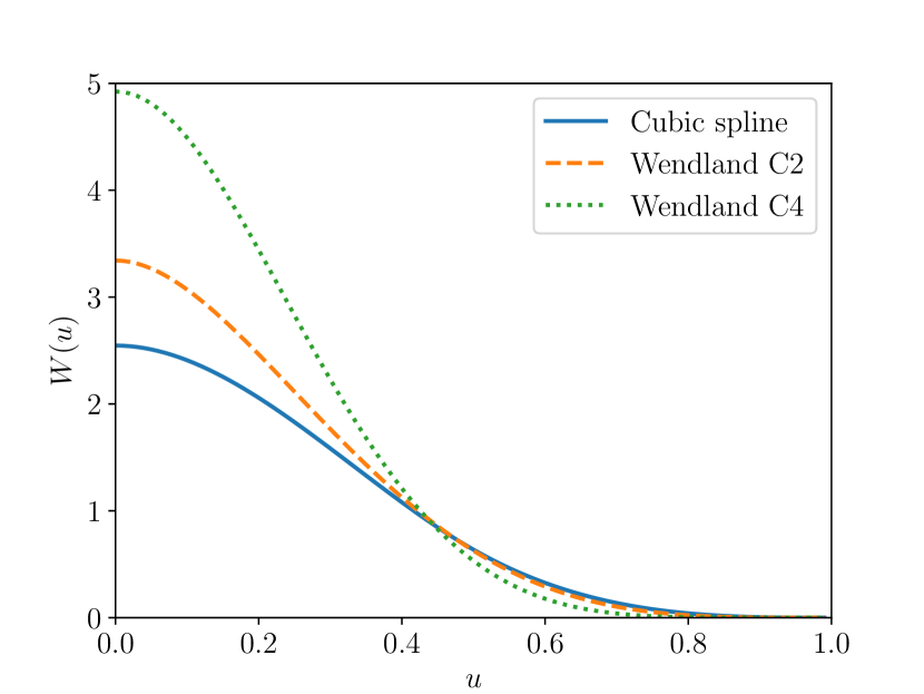
In our simulations we employ 3 different kernel functions. The first is the standard cubic spline kernel (Monaghan & Lattanzio, 1985):

$$W(u,h_{i})=\frac{8}{\pi h_{i}^{3}}\begin{cases}1+6u^{2}(u-1)&\mathrm{for}~{}0\leq u<\frac{1}{2},\\ 2(1-u)^{3}&\mathrm{for}~{}\frac{1}{2}\leq u<1,\\ 0&\mathrm{otherwise},\end{cases}$$ (17)

where $h_{i}$ is the kernel size (or smoothing length) of a fluid element, and $u$ is defined as $u\equiv|\bm{x}-\bm{x_{i}}|/h_{i}$, where $\bm{x}_{i}$ is the position of the fluid element. Modern SPH prescriptions often employ higher order Wendland functions (Wendland, 1995) as kernels to avoid the well-known paring instability when using a large number of neighbours, which is preferable as it reduces low-order errors in the SPH method (Dehnen & Aly, 2012). In this paper, we employ the Wendland C2 and C4 kernels in addition to the standard cubic spline kernel. The functional form of the three-dimensional Wendland C2 kernel is:

$$W(u,h_{i})=\frac{21}{2\pi h^{3}_{i}}\begin{cases}(1-u)^{4}(1+4u)&\mathrm{for}~{}0\leq u<1,\\ 0&\mathrm{otherwise},\end{cases}$$ (18)

and that of the Wendland C4 kernel is:

$$W(u,h_{i})=\frac{495}{32\pi h^{3}_{i}}\begin{cases}(1-u)^{6}(1+6u+\frac{35}{3}u^{2})&\mathrm{for}~{}0\leq u<1,\\ 0&\mathrm{otherwise}.\end{cases}$$ (19)

These three kernel functions used in this study are shown in Fig. 1, which clearly shows that the higher-order Wendland kernels are more centrally concentrated than the cubic spline. Since higher-order kernels assign more weight to closer fluid elements, they generally require higher values of $N_{\mathrm{NEIB}}$ to correctly reproduce the actual fluid density (Dehnen & Aly, 2012).

In GIZMO, the kernel size, $h_{i}$, is determined such that the smoothed number density of fluid elements, $n(\bm{x}_{i})$, is constant (see also Springel & Hernquist 2002), given by:

$$n(\bm{x}_{i})\equiv\sum_{j}W(|\bm{x}_{j}-\bm{x}_{i}|/h_{i},h_{i})=\frac{N_{\mathrm{NEIB}}}{(3/4)\pi h_{i}^{3}}.$$ (20)

which is solved iteratively for $h_{i}$. The density of an SPH particle is then:

$$\rho_{i}^{\mathrm{SPH}}=\sum_{j}m_{j}W(|\bm{x}_{j}-\bm{x}_{i}|/h_{i},h_{i}),$$ (21)

where $m_{j}$ is the mass of the $j$-th SPH particle. In MFM and MFV, the density of a fluid element is defined instead as

$$\rho_{i}^{\mathrm{MFM/MFV}}=m_{i}n(\bm{x}_{i}),$$ (22)

because $n(\bm{x}_{i})^{-1}$ is the volume of the fluid element in these two schemes. When fluid elements all have the same mass, as in our initial conditions, these two definitions above are identical.

2.4 The definition of resolution

As in Hubber et al. (2006), we define the minimum resolvable mass as $M_{\mathrm{MIN}}=N_{\mathrm{NEIB}}m$. The Jeans condition states that the Jeans mass $M_{\mathrm{J}}$ must exceed $M_{\mathrm{MIN}}$, that is,

$$M_{\mathrm{MIN}}=N_{\mathrm{NEIB}}m\leq M_{\mathrm{J}}=\frac{4}{3}\pi\left(\frac{\lambda_{\mathrm{J}}}{2}\right)^{3}\rho=\frac{\pi^{5/2}c_{\mathrm{s}}^{3}}{6G^{3/2}\rho^{1/2}}.$$ (23)

This condition can also be read as effectively setting a density threshold of:

$$\rho\leq\left(\frac{\pi}{6N_{\mathrm{NEIB}}m}\right)^{2}\left(\frac{\pi c_{s}^{2}}{G}\right)^{3}.$$ (24)

By using Eq.(15) as the kernel size, we derive the following condition,

$$\lambda_{\mathrm{J}}\geq 2\bar{h},$$ (25)

namely, the Jeans wavelength should exceed the diameter of a fluid element. This Jeans Condition is identical to that used in Hubber et al. (2006).

We define the resolution, $\mathcal{R}$, as a ratio of the mean diameter of a fluid element, $\bar{d}=2\bar{h}$, to the wavelength of the perturbation, $\lambda=n^{-1}_{\lambda}$, where $n_{\lambda}$ is the integer number of wavelengths that fit within a side of the simulation box (of length $=1$), i.e.

$$\mathcal{R}=\frac{\bar{d}}{\lambda}=n_{\lambda}2\bar{h}=n_{\lambda}\left(\frac{6{N}_{\mathrm{NEIB}}}{\pi N_{\mathrm{tot}}}\right)^{1/3}.$$ (26)

A smaller value of $\mathcal{R}$ corresponds to better resolution. For $\lambda=\lambda_{\mathrm{J}}$, the Jeans condition (Eq. (25)) reads:

$$\mathcal{R}\leq 1.$$ (27)

For the tests presented in the following sections, we fix the perturbation wavelength at each resolution and alter the ratio $\lambda/\lambda_{\mathrm{J}}$ by changing the isothermal sound speed, $c_{\mathrm{s}}$.

3 Results

Figure 2: The density fluctuation, $\delta$, as a function of $x$-position of each fluid element when the maximum density fluctuation, $\max\{\delta_{i}(t)\}$, reaches $\cosh(1)$ times the initial maximum density perturbation, $\max\{\delta_{i}(t=0)\}$. The resolution of each simulation is $\mathcal{R}=0.25$ and the wavelength of a perturbation is $\lambda/\lambda_{\mathrm{J}}=1.2$. The upper-left, upper-right, lower-left, and lower-right panels present the results of TSPH, PSPH, MFM, and MFV, respectively. The blue solid line shows the density fluctuation obtained by multiplying the initial density fluctuation by $\cosh(1)$.

In this section we report the results of the simulations outlined in Section 2. We measure the oscillation period for small scale perturbations ($\lambda<\lambda_{\mathrm{J}}$) and the characteristic timescale for the maximum density fluctuation to increase by $\cosh(1)$ for the larger scale perturbations that trigger collapse ($\lambda<\lambda_{\mathrm{J}}$), and compare both to the analytic solutions of Eq. (11) and Eq. (12).

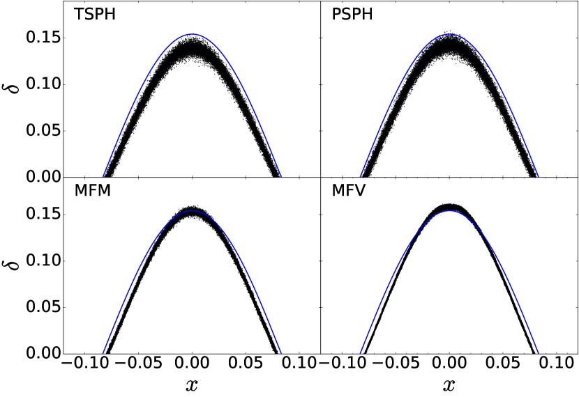
In Fig. 2, we show the density fluctuations of the fluid elements against their $x$-positions when the maximum density fluctuation, $\delta^{\mathrm{max}}(t)\equiv\max\{\delta_{i}(t)\}$, in the simulation box reaches $\cosh(1)$ times the initial maximum density fluctuation, $\delta^{\mathrm{max}}(t=0)$, for the four different hydrodynamical schemes for the specific case of $\mathcal{R}=0.25$ (well-resolved) and $\lambda/\lambda_{\mathrm{J}}=1.2$ (collapsing).

We find that, due to the large noise in SPH, the maximum density in TSPH and PSPH does not represent the typical density at the location of the peak. Because of this, we underestimate the characteristic timescale for SPH when we simply use the maximum density. On the other hand, the density distribution in MFV is very tight, indicating that MFV is the least diffusive method of the four. Note that the initial density fields are identical in all simulations.

To circumvent this problem, we evaluate the mean density at the $x$-position of a fluid element, $i$, by using fluid elements within $0.1h_{i}$, i.e. $|x_{j}-x_{i}|<0.1h_{i}$. Doing so makes the density distribution a single-valued function of $x$ and we avoid the bias caused by the noisy density field present in the SPH methods. We call this density $\tilde{\rho}$ to discriminate it from the density of a fluid element. We also define $\tilde{\delta}$ as the density fluctuation computed from $\tilde{\rho}$. This mean density, $\tilde{\rho}$, is used to define all the growth timescales quoted in this paper.

3.1 Comparisons between different Lagrangian methods

Figure 3: Oscillation periods for $\lambda<\lambda_{\mathrm{J}}$ and growth time scales for $\lambda>\lambda_{\mathrm{J}}$ as functions of the perturbation wavelength normalised by the Jeans wavelength. The circles, stars, upward triangles and downward triangles, respectively, indicate results from the MFM, MFV, TSPH, and PSPH methods. The analytic solutions, Eq. (11) and Eq. (12), are represented by the solid lines. In panels (a), (b), (c), and (d), we present results with the resolution, $\mathcal{R}=0.25$, 0.5, 1, and 2, respectively.

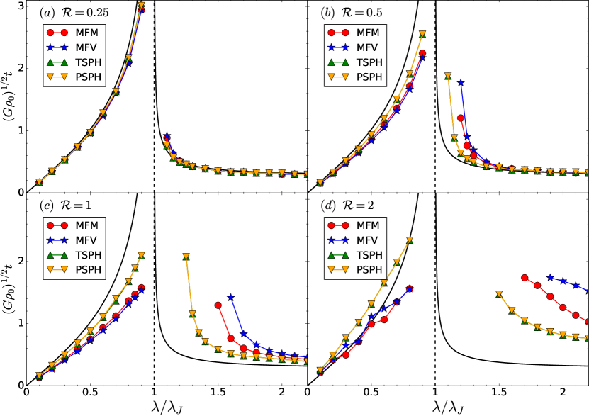
In Fig. 3, we show the results of our Jeans test simulations. In all simulations presented here, we employ the cubic spline kernel and $N_{\mathrm{NEIB}}=50$. Firstly, we confirm the earlier results by Hubber et al. (2006), that is, (i) perturbations which should oscillate ($\lambda<\lambda_{\mathrm{J}}$) always oscillate and do not display artificial fragmentation even when the Jeans mass is not resolved ($\mathcal{R}=2$), (ii) poor resolution stabilizes unstable perturbations ($\lambda>\lambda_{\mathrm{J}}$) near $\lambda\sim\lambda_{\mathrm{J}}$ and the wavelength of the perturbations that fail to grow becomes longer with poorer resolution (i.e. larger $\mathcal{R}$), and (iii) poorer resolution makes the growth timescale longer for a given wavelength.

Comparing the results from the four different schemes, TSPH and PSPH are indistinguishable at all resolutions. This is always true in the simulations presented in this paper, and hence we hereafter simply refer to them collectively as SPH. In the highest resolution simulations ($\mathcal{R}=0.25$), the characteristic timescales obtained with different schemes nicely converges to the analytic timescales and there is little difference between them.

In lowering the resolution the numerical results deviate from the analytic estimates.Except for the oscillating perturbations in the lowest resolution simulations ($\lambda<\lambda_{\mathrm{J}}$ and $\mathcal{R}=2$), the results with SPH are closer to the analytic estimates than MFM and MFV. The oscillation periods with MFV are shorter than those with SPH for $\lambda<\lambda_{\mathrm{J}}$ and the growth timescales with MFV are longer than those with SPH, indicating that the ratio of the magnitude of the hydrodynamic force to that of self-gravitational force in MFV is larger than in SPH. The results with MFM consistently lie between SPH and MFV, and always closer to MFV.

For the growing perturbations, the growth timescale described by Eq. (12) is a downwardly convex function. When the perturbation is not resolved ($\mathcal{R}=2$), the growth timescale with MFV does not display this characteristic form, while the curve obtained with SPH is still downwardly convex at this resolution. MFM is somewhat ambiguous at this resolution, while generally exhibiting the desired downwardly convex behaviour. This may suggest some unphysical behaviour of MFV when the Jeans condition is violated. We shall revisit this issue in Section 3.3.

3.2 Comparisons with different kernel functions

Figure 4: The growth timescales with different kernel functions and the MFM method. The circles, stars, and triangles indicate the results with the cubic spline, Wendland C2, and Wendland C4 kernels, respectively. Form left to right, the resolutions adopted are $\mathcal{R}=0.5$, 1.0, and 2.0.

Figure 5: The growth timescales with several combinations of the kernel functions and the number of neighbour particles. The circles and stars represent the results by the cubic spline and Wendland C4 kernels, respectively. For the cubic spline kernel, the line connecting the symbols closer to the analytic estimate indicates the results with $N_{\mathrm{NEIB}}=30$ and the other line with $N_{\mathrm{NEIB}}=64$. For the Wendland C4 kernel, the lines indicate $N_{\mathrm{NEIB}}=60$, 128, and 180 from the closet to the analytic estimate to the farthest, respectively.

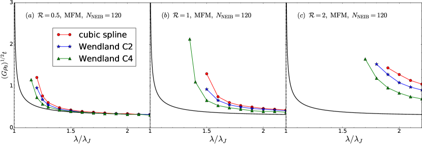
In this subsection, we again carry out the Jeans test, but now investigating the effect of changing the kernel function. We employ MFM as the hydrodynamic scheme in this subsection. Firstly, we fix $N_{\mathrm{NEIB}}$ to 120 to focus on the effect of different kernel shapes. This number of neighbours is typical for the Wendland C4 kernel, and may otherwise cause the paring instability if used with the cubic spline kernel in SPH (e.g. Dehnen & Aly, 2012). MFM and MFV should be free from this problem and we can safely use the cubic spline kernel with such a large number of neighbours (Hopkins, 2015).

In Fig.4, we show the growth timescales with the cubic spline, Wendland C2, and Wendland C4 kernels by changing the resolution from $\mathcal{R}=0.5$ to 2.0. The results with MFM are similar to those shown in Fig. 3. For a given resolution, $\mathcal{R}$, the timescales obtained with the higher-order kernels are closer to the analytic estimate than their lower-order counterparts. As is evident from Fig. 1, higher-order kernels are more centrally concentrated than lower-order ones and therefore allocate more weight to closer fluid elements. Also, the gravitational force is less softened by the higher-order kernels for a given kernel size.

Our results indicate that defining resolution as the ratio of the mean diameter or kernel size of a fluid element to the local Jeans wavelength is not appropriate when several kernel functions are in use. It is therefore convenient to introduce a definition of resolution that is independent of the kernel function.

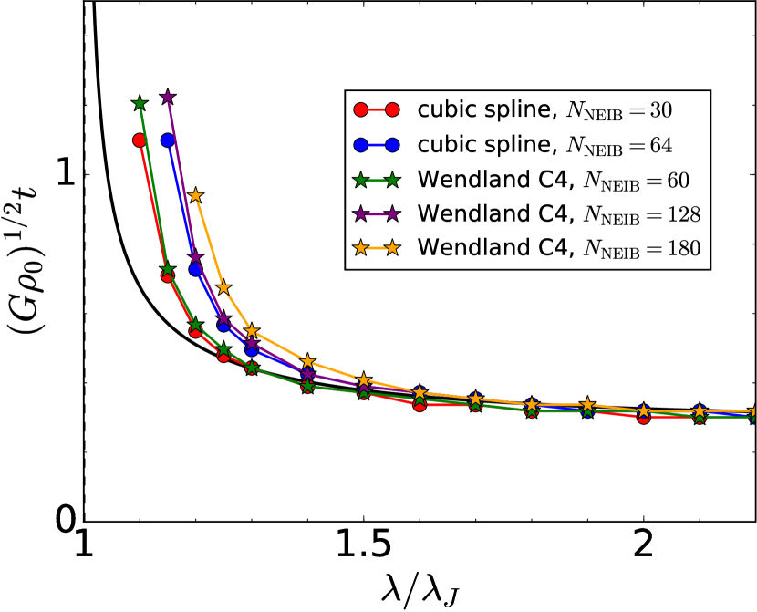
We compare the growth timescales with the cubic spline and Wendland C4 kernels by changing $N_{\mathrm{NEIB}}$ in Fig. 5, in which we use $N_{\mathrm{NEIB}}=30$ and $64$ for the cubic spline kernel and $N_{\mathrm{NEIB}}=60$, 128 and 180 for the Wendland C4 kernel.

We find that the results using the cubic spline kernel with $N_{\mathrm{NEIB}}=30$ and 64 are almost identical to those by the Wendland C4 kernel with $N_{\mathrm{NEIB}}=60$ and 128, respectively. This indicates that the resolutions $\mathcal{R}\simeq 0.32$ and 0.41 for the cubic spline kernel roughly correspond to $\mathcal{R}\simeq 0.4$ and 0.51 for the Wendland C4 kernel, respectively. In other words, the effective kernel size of the cubic spline kernel is $\sim 2^{1/3}=1.26$ times as large as that of the Wendland C4 kernel for a given kernel size.

Dehnen & Aly (2012) defined the effective hydrodynamic resolution as the kernel standard deviation, $\sigma$:

$$\sigma^{2}=\nu^{-1}\int\mathrm{d}^{\nu}x\ \bm{x}^{2}W(|\bm{x}|/h,h),$$ (28)

where $\nu$ is the number of spatial dimensions. The effective smoothing length $h^{\prime}$ is then defined as

$$h^{\prime}=2\sigma.$$ (29)

The ratio of the effective smoothing length to the kernel size, $h^{\prime}/h$, is $\simeq 0.5477$ and $\simeq 0.4529$ for the cubic spline and Wendland C4 kernels, respectively (Dehnen & Aly, 2012). The effective smoothing length of the cubic spline kernel is thus $\sim 1.21$ times as large as that of the Wendland C4 kernel for a given kernel size. This scaling is similar to that indicated by Fig. 5. Since the effective smoothing length is about half the kernel size, we can define the effective resolution, $\mathcal{R}^{\prime}$, in a kernel-independent manner as

$$\mathcal{R}^{\prime}=\frac{4h^{\prime}}{\lambda}.$$ (30)

The results shown in Fig. 3 can be applied to other kernels by replacing $\mathcal{R}$ with $\mathcal{R}^{\prime}=1.095\mathcal{R}$.

3.3 Effects of the amplitude of initial perturbations

Figure 6: The initial density fluctuation at each resolution. The density fluctuation of each fluid element is shown against its $x$-position by black points. The blue solid line represents the target density fluctuation given by Eq. (13) with $A=0.1$. The panels (a), (b), (c), and (d) show the initial conditions for resolutions of $\mathcal{R}=0.25$, 0.5, 1, and 2, with the cubic spline kernel, respectively.

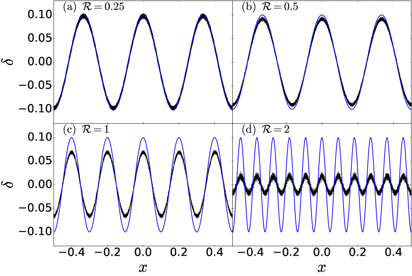
So far, we have used the same coordinate transformation as Hubber et al. (2006) to generate the initial perturbations (Eq. (16)). The initial perturbations added in this way, however, depend on the resolution. In Fig. 6, we show the density fluctuation of each fluid element with the cubic spline kernel and the target density given by Eq. (13) with $A=0.1$. We find that the higher the resolution, the better the target initial condition is reproduced. At the lowest resolution, $\mathcal{R}=2$, the amplitude is only one-third of the target amplitude due to the kernel size being much larger than the wavelength of the perturbations. This small amplitude should not affect our measure of the timescales because we define the characteristic growth timescale as the time at which the maximum density fluctuation reaches $\cosh(1)$ times the initial maximum density fluctuation. Nevertheless, it is interesting to investigate the response when the imposed initial density perturbation more accurately matches the targeted amplitude.

Figure 7: The same as Fig. 6 but showing the revised initial condition for $\mathcal{R}=2$.

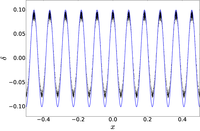
To generate an appropriate density distribution, we evolve the system by adjusting the pressure of each fluid element without self-gravity. When a fluid element has higher/lower density than the target density at its position, $x$, we increase/decrease its pressure according to the following equation:

$$P_{i}=\bar{P}\left(1+\Delta\frac{\rho_{i}-\rho_{\mathrm{t}}(x_{i})}{\lambda}\right),$$ (31)

where $\rho_{\mathrm{t}}(x_{i})$ is the target density at the position of the $i$-th particle given by Eq. (16) with $A=0.1$, $\bar{P}$ is the reference pressure which we can arbitrarily determine, and $\Delta$ is a adjustable parameter. We start from the original initial condition and evolve the system by adjusting the pressure through Eq. (31) with relatively large values $\Delta$. We then gradually decrease the value of $\Delta$ until the total relative variation, $\sum_{i}|\rho_{i}-\rho_{\mathrm{t}}(x_{i})|/\rho_{\mathrm{t}}(x_{i})$, cannot become smaller anymore.

We show the density fluctuation obtained by this procedure in Fig. 7 for $\mathcal{R}=2$. The density distribution is now much closer to the target density than the original initial condition obtained by the coordinate transformation of Eq. (16).

Figure 8: The same as Fig. 3 but with the revised initial conditions. Only the results for $\mathcal{R}=2$ are shown.

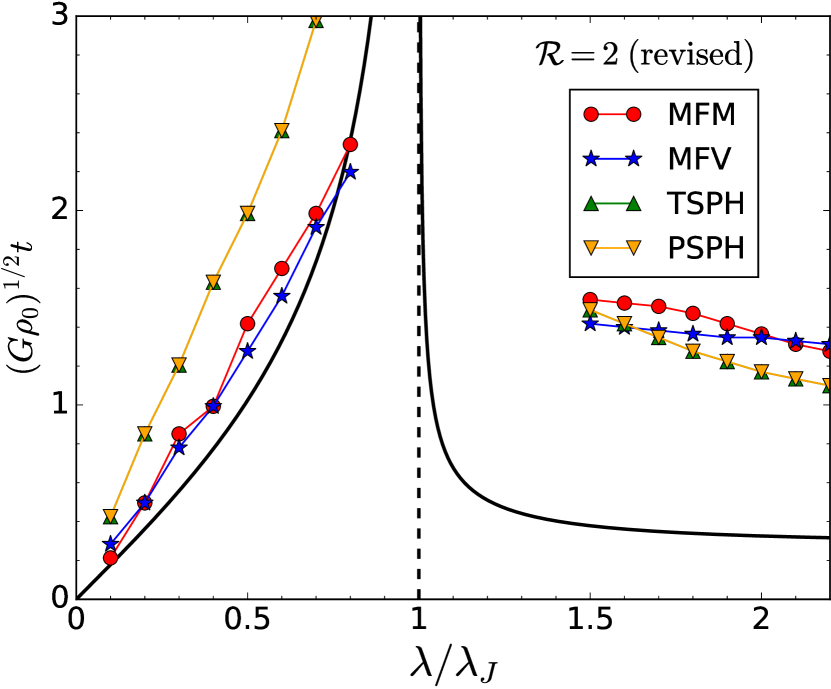
Using initial conditions generated in this manner, we again perform the Jeans test simulations and vary the hydrodynamical scheme. We show the results in Fig. 8. We find that the results noticeably change from the ones shown in Fig. 3.

For the short wavelength perturbations ($\lambda<\lambda_{J}$), the oscillation periods become longer than those with the original initial conditions, while the slopes of the timescales as functions of wavelength are maintained. For the long wavelength perturbations $(\lambda_{J}<\lambda)$, the difference between the hydrodynamic methods becomes smaller than that shown in Fig. 3. The timescales obtained with MFV are almost independent of wavelength.

Figure 9: The time evolution of the density fluctuation profile in a simulation with MFV. We use the cubic spline kernel and a resolution of $\mathcal{R}=2$, with an initial perturbation of $\lambda/\lambda_{\mathrm{J}}=1.5$. We also show the initial density fluctuation given by Eq. (13) with $A=0.1$ as blue solid lines. The time is expressed as $\tau=(G\rho_{0})^{1/2}t$.

Figure 10: The density fluctuation profiles, $\tilde{\delta}(x)$, when the maximum density fluctuation reaches $\cosh(1)$ times the initial maximum density fluctuation at the resolution of $\mathcal{R}=2$ with the cubic spline kernel. From top to bottom, the results are shown using the TSPH, MFM, and MFV methods, respectively. The blue solid line indicates the density field obtained by multiplying the density fluctuation in Eq. (13) by $\cosh(1)$.

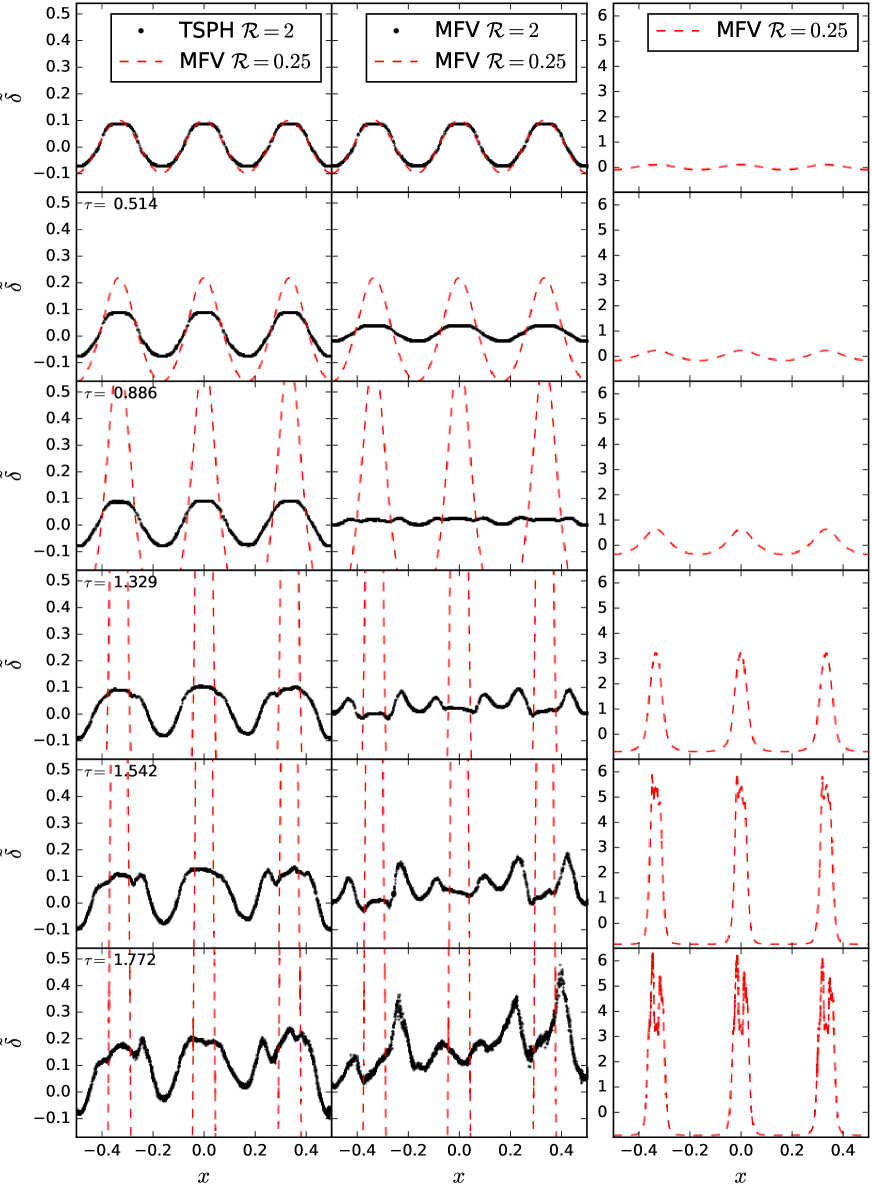
To understand this odd behaviour in the growth timescale when using MFV, we show the explicit time evolution of $\tilde{\delta}(x)$ of the fluid elements with position, $x$, in Fig. 9. The resolution is $\mathcal{R}=2$ and the wavelength of the perturbation is $\lambda/\lambda_{\mathrm{J}}=1.5$.

We find that the perturbations initially do not grow but decay. They almost disappear by $\tau=0.886$, then shorter wavelength perturbations start to grow (see $\tau=1.329$). These density fluctuations are the ones that reach $\cosh(1)$ times the initial maximum density fluctuation when we define the characteristic timescale. We note that we do not observe this behaviour of initial decay and subsequent fragmentation into short-wavelength perturbations when we run simulations from the original initial conditions, in which the amplitude of the initial perturbation is much smaller than intended. (see Fig. 6 (d)). When the amplitude of the unresolved perturbation with $\lambda>\lambda_{J}$ is too small as the original one and its wavelength is close to the Jeans length, the perturbation oscillates.

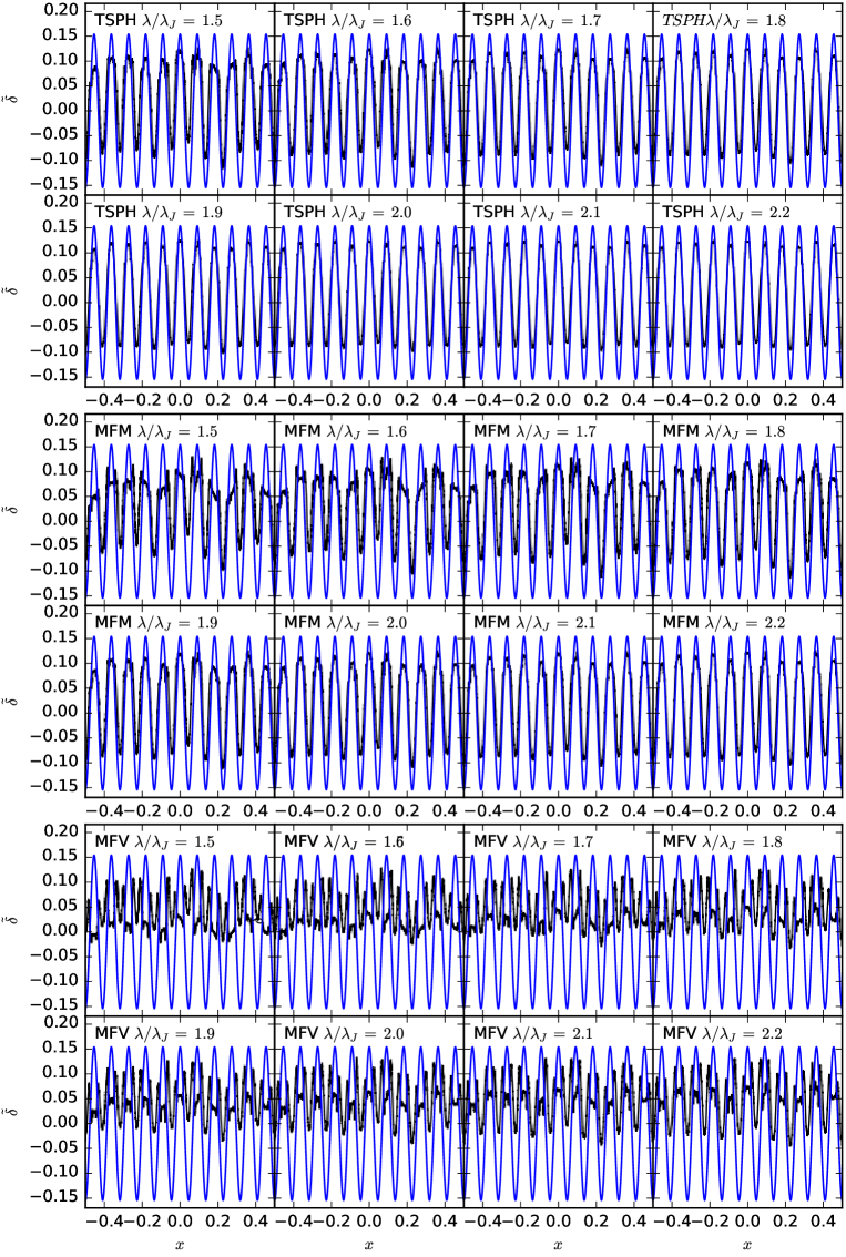
In Fig. 10, we show the density fluctuation profiles, $\tilde{\delta}(x)$, at the final epoch, at which $\delta^{\mathrm{max}}(t)=\cosh(1)\delta^{\mathrm{max}}(t=0)$), with TSPH, MFM, and MFV with changing perturbation wavelength in the range of $\lambda/\lambda_{\mathrm{J}}=1.5$ to 2.2. We find that results with TSPH are robust, at least the sinusoidal shapes are always maintained, even when we strongly violate the Jeans condition; only a slight signature of wave deformation is seen when the perturbation wavelength is close to the Jeans length. With MFV, perturbations always strongly deform and the density peaks are not located at those in the initial conditions, even when the perturbation wavelength is 2.2 times the Jeans length. MFM again shows an intermediate behaviour between SPH and MFV, though closer to that of SPH.

To show that the fluctuations in the unresolved simulations indeed do not oscillate but actually grow as expected, we show the longer timescale evolution in Fig. 11. We show TSPH and MFV simulations with low resolution $\mathcal{R}=2$ and a perturbation wavelength of $\lambda/\lambda_{\mathrm{J}}=1.5$. We also show a higher resolution simulation (with $\mathcal{R}=0.25$) with MFV for a comparison of the expected perturbation growth. We multiply the $x$-positions of the low resolution simulations ($\mathcal{R}=2$) by 3/11 so that the wavelength of the perturbation matches that of the resolved simulation, for ease of comparison.

With SPH, the initial density perturbation slowly grows, keeping its sinusoidal shape. The growth is, however, much slower than that of the well-resolved simulation (red dashed lines). These perturbations fragment into shorter wavelength perturbations after $\tau\simeq 1.54$.

With MFM, as we mentioned before, the initial density perturbation fails to grow. The newly developed density perturbations keep growing and the peak density fluctuation is higher than with SPH at $\tau=1.772$. The peak density is, of course, much smaller than in the resolved simulation; the difference is more than an order of magnitude.

Note that, even in the well-resolved run, the growth is slowed when density reaches too high to resolve the Jeans length with this resolution because, for isothermal gas, the Jeans length, $\lambda_{\mathrm{J}}\propto\rho^{-1/2}$, is a faster decreasing function of density than the kernel size, $h\propto\rho^{-1/3}$. When the density becomes too high, fragmentation into smaller wavelengths is also observed for this simulation, as we would expect from the behaviour of the lower resolution simulations.

We have confirmed that, in all these simulations, the density perturbations grow until the timesteps become too small and the code ultimately crashes.

Figure 11: The time evolution of the density fluctuation profiles , $\tilde{\delta}(x)$, in SPH and MFV are shown in the left and middle columns, respectively, as black dots. The resolution for these simulations is $\mathcal{R}=2$ and the perturbation wavelength is $\lambda/\lambda_{\mathrm{J}}=1.5$. We also show the resolved simulation ($\mathcal{R}=0.25$) with MFV as red dashed lines to show the ideal well-resolved growth rate. For an easier comparison, we have multiplied the $x$-position of the low resolution simulation ($\mathcal{R}=2$) by 3/11 so that the wavelength of the perturbation matches that of the resolved simulation. In the right column we show the resolved simulation but with the full vertical scale for reference. From top to bottom, the times are $\tau=0,0.514,0.886,1.329,1.542,$ and $1.772$, respectively.

4 Discussion and conclusions

We have carried out the Jeans test using Lagrangian hydrodynamic schemes implemented in GIZMO: TSPH, PSPH, MFM, and MFV. We have confirmed that the TSPH results are consistent with those of Hubber et al. (2006). The PSPH results are indistinguishable from those with TSPH, reflecting that the Jeans test does not involve any discontinuities or shear flows.

Using the cubic spline kernel, the oscillation periods and the growth timescales with all the methods converged to the analytic estimates at a resolution of $\mathcal{R}=0.25$, where $R$ is the ratio of kernel diameter to perturbation wavelength. At $\mathcal{R}<1$, the oscillation period becomes shorter and the growth timescale longer as the resolution is decreased. Convergence to the analytic solution is fastest with the SPH methods and slowest with MFV. In all the test simulations, MFM shows a behaviour intermediate between SPH methods and MFV.

Unlike Eulerian methods such as AMR, even when we strongly violate the Jeans condition (e.g. $\mathcal{R}=2$), none of the four schemes show artificial fragmentation for shorter wavelength perturbations with $\lambda<\lambda_{\mathrm{J}}$, i.e. perturbations with a wavelength shorter than the Jeans length never fragment. This result is consistent with the SPH-specific investigation of Hubber et al. (2006). We suspect that one of the reasons why the Lagrangian methods behave differently from AMR is that, in the Lagrangian methods we have tested here, the spatial and mass resolution are directly coupled, whereas, in AMR, the relation between the two depends on the refinement criteria.

Longer wavelength perturbations ($\lambda>\lambda_{\mathrm{J}}$), however, grow quite differently from the converged behaviour with MFM when we fail to satisfy the Jeans condition. Initially imposed perturbations fail to grow and waves are reflected at the density peaks. Newly formed density perturbations during the initial density peaks then grow and collapse. Interestingly, SPH shows more consistent behaviour with the converged simulations even when the Jeans condition is violated. Initially imposed perturbations grow, although the growth is much slower than in the resolved cases, and the fragmentation into shorter wavelength fluctuations occurs slower than in the equivalent MFV simulation.

Our results suggest that, when unresolved, the ratio of the magnitude of hydrodynamic force to that of self-gravity at sub-resolution scale is the largest in MFV and smallest in SPH. This sub-resolution scale pressure gradient force in MFV overcomes the softened self-gravitational force when we impose unresolved strongly nonlinear initial density perturbations. The spectrum between the three Lagrangian methods is consistent with the fundamentals of the schemes. Of the three, MFV is the closest to Eulerian methods in the way that it employs a finite volume method with a Riemann solver like AMR, with inter-cell mass fluxes. MFM lies between SPH and MFV: like MFV, MFM uses a finite volume method with a Riemann solver, but it is similar to SPH in that there is no inter-cell mass flux.

The difference between SPH and MFV when we impose strongly non-linear unresolved perturbations may be consistent with the kernel-scale difference in dissipation and noise in SPH and MFV demonstrated in Hopkins (2015, Section 4.4.4). In the power spectrum of driven, isothermal turbulence, they find a ‘bottleneck’ feature (excess power on scales just above the dissipation range) in MFM and MFV simulations. On the other hand, with SPH, the power spectrum falls below the expected value. The differences between SPH and MFV are qualitatively similar to the difference we report here. In their test, however, MFM and MFV behave indistinguishably. This is in contrast to our results, in which MFM is qualitatively more similar to SPH than MFV (see Fig. 10). The main difference between finite mass methods like SPH and MFM and finite volume methods like MFV (and AMR) is the existence of the inter-cell mass fluxes. In a method with mass fluxes where gravity and hydro are operator split, it is difficult to maintain hydrostatic equilibrium (e.g. Zingale et al., 2002). To realise the hydrostatic equilibrium with such a method, large hydrodynamic fluxes and gravity need to cancel out each other; achieving this is difficult with the finite volume method in general. On the other hand, in SPH and MFM, the gravitational force is calculated in a point-like manner, approximating a fluid element as a point mass. This means that in a method like SPH where the fluid forces are also evaluated in a point-like collocated manner one can get much better force cancellation. In MFM the introduction of the Riemann solver and the finite-volume method would lead to some deviations. It, however, still has velocity collocation (i.e. no mass fluxes), and this may help to achieve hydrostatic equilibrium.

We also find that our results obtained with the cubic spline kernel can be generalised to other kernels by using the effective smoothing length, $h^{\prime}=2\sigma$, where $\sigma$ is the kernel standard deviation defined by Eq. (28). By using this effective smoothing length, we can define the kernel-independent resolution, $\mathcal{R}^{\prime}$, as $\mathcal{R}^{\prime}=4h^{\prime}/\lambda$. To follow the growth of a perturbation whose wavelength is close to the Jeans length with the cubic spline kernel, the resolution required is $\mathcal{R}=0.25$. This corresponds to $\mathcal{R}^{\prime}\simeq 0.28$ and all the schemes tested here produce almost identical results at this resolution.

Data Availability

The data underlying this article will be shared on reasonable request to the corresponding author.

References

- Agertz et al. (2007) Agertz O., et al., 2007, MNRAS, 380, 963
- Bate & Burkert (1997) Bate M. R., Burkert A., 1997, MNRAS, 288, 1060
- Bate et al. (2002) Bate M. R., Bonnell I. A., Bromm V., 2002, MNRAS, 332, L65
- Dehnen & Aly (2012) Dehnen W., Aly H., 2012, MNRAS, 425, 1068
- Duffell & MacFadyen (2011) Duffell P. C., MacFadyen A. I., 2011, The Astrophysical Journal Supplement Series, 197, 15
- Gaburov & Nitadori (2011) Gaburov E., Nitadori K., 2011, MNRAS, 414, 129
- Gingold & Monaghan (1977) Gingold R. A., Monaghan J. J., 1977, MNRAS, 181, 375
- Hopkins (2013) Hopkins P. F., 2013, MNRAS, 428, 2840
- Hopkins (2015) Hopkins P. F., 2015, MNRAS, 450, 53
- Hubber et al. (2006) Hubber D. A., Goodwin S. P., Whitworth A. P., 2006, A&A, 450, 881
- Hubber et al. (2018) Hubber D. A., Rosotti G. P., Booth R. A., 2018, MNRAS, 473, 1603
- Jeans (1929) Jeans J. H., 1929, Astronomy and Cosmology. Cambridge, UK: Cambridge University Press
- Kawata et al. (2013) Kawata D., Okamoto T., Gibson B. K., Barnes D. J., Cen R., 2013, MNRAS, 428, 1968
- Lucy (1977) Lucy L. B., 1977, ApJ, 82, 1013
- Monaghan & Lattanzio (1985) Monaghan J. J., Lattanzio J. C., 1985, A&A, 149, 135
- Okamoto et al. (2003) Okamoto T., Jenkins A., Eke V. R., Quilis V., Frenk C. S., 2003, MNRAS, 345, 429
- Price (2008) Price D. J., 2008, Journal of Computational Physics, 2271, 10040
- Price & Monaghan (2007) Price D. J., Monaghan J. J., 2007, MNRAS, 374, 1347
- Read et al. (2010) Read J. I., Hayfield T., Agertz O., 2010, MNRAS, 405, 1513
- Ritchie & Thomas (2001) Ritchie B. W., Thomas P. A., 2001, MNRAS, 323, 743
- Saitoh & Makino (2013) Saitoh T. R., Makino J., 2013, ApJ, 768, 44
- Springel (2010) Springel V., 2010, MNRAS, 401, 791
- Springel & Hernquist (2002) Springel V., Hernquist L., 2002, MNRAS, 333, 649
- Truelove et al. (1997) Truelove J. K., Klein R. I., McKee C. F., Holliman II J. H., Howell L. H., Greenough J. A., 1997, ApJ, 489, L179
- Wadsley et al. (2008) Wadsley J. W., Veeravalli G., Couchman H. M. P., 2008, MNRAS, 387, 427
- Wendland (1995) Wendland H., 1995, Advances in Computational Mathematics, 4, 389
- Yalinewich et al. (2015) Yalinewich A., Steinberg E., Sari R., 2015, ApJS, 216, 35
- Zingale et al. (2002) Zingale M., et al., 2002, The Astrophysical Journal Supplement Series, 143, 539