Few-shot Learning for Topic Modeling

Abstract

Topic models have been successfully used for analyzing text documents. However, with existing topic models, many documents are required for training. In this paper, we propose a neural network-based few-shot learning method that can learn a topic model from just a few documents. The neural networks in our model take a small number of documents as inputs, and output topic model priors. The proposed method trains the neural networks such that the expected test likelihood is improved when topic model parameters are estimated by maximizing the posterior probability using the priors based on the EM algorithm. Since each step in the EM algorithm is differentiable, the proposed method can backpropagate the loss through the EM algorithm to train the neural networks. The expected test likelihood is maximized by a stochastic gradient descent method using a set of multiple text corpora with an episodic training framework. In our experiments, we demonstrate that the proposed method achieves better perplexity than existing methods using three real-world text document sets.

1 Introduction

There is great interest in topic modeling, such as latent Dirichlet allocation [8] and probabilistic latent semantic analysis [22], for analyzing text documents, which include scientific papers, news articles, and web pages [6, 7, 19, 40, 27, 41, 10, 13, 59, 11, 40]. A topic model is a probabilistic generative model, in which a document is modeled as a mixture of topics, and a topic is modeled as a probability distribution over vocabulary terms. Topic models have been successfully used in a wide variety of applications including information retrieval [8], collaborative filtering [23], visualization [28], and entity disambiguation [30].

For estimating topic models, many documents are required. However, some applications may have insufficient numbers of documents. In this paper, we propose a few-shot learning method for topic modeling, which can estimate topic models from just a small number of documents. Although many few-shot learning methods have been proposed [50, 4, 45, 2, 54, 51, 3, 16], existing few-shot learning methods are not intended for topic modeling.

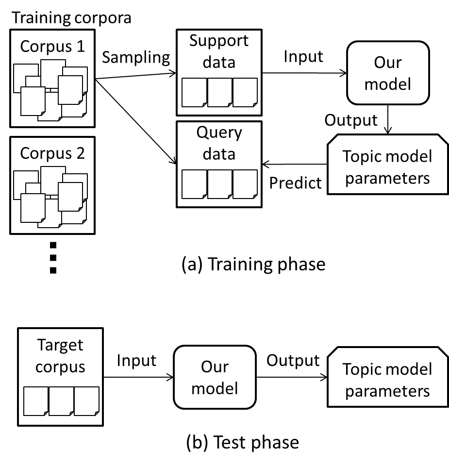
The proposed method uses a neural network-based model that generates topic model parameters. In the training phase, we are given a set of multiple text corpora, where each corpus is assumed to be generated from a topic model with corpus-specific parameters. We train our model by maximizing the expected test log-likelihood using the training corpora with an episodic training framework [49], where support and query data are randomly sampled from training corpora to simulate the test phase for each epoch. The support data are used for generating a corpus-specific topic model, and the query data are used for evaluating the generated topic model. In the test phase, we are given a small number of documents, which are support data, in the target corpus. Our aim is to estimate a topic model for the given target corpus. Figure 1 shows our framework.

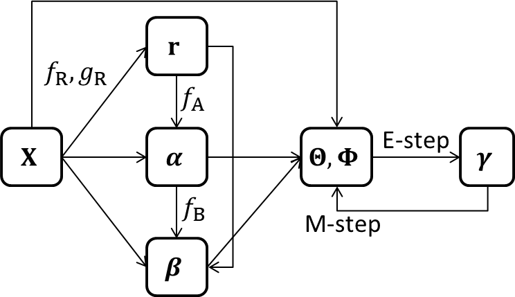
The neural networks in our model take support data as input, and output topic model priors. First, our model obtains a corpus representation by a permutation invariant neural network [58] from the support data. The corpus representation contains the property of the support data. Next, Dirichlet parameters, which define the prior distribution of topic model parameters, are obtained by neural networks using the corpus representation and support data. By using the corpus representation, the obtained Dirichlet parameters become corpus-specific. Then, topic model parameters are obtained by maximizing the posterior probability given the support data and the priors with the expectation-maximization (EM) algorithm [12]. Each step in the EM algorithm can be seen as a layer of a neural network in our model. Since our model is differentiable, including the EM steps, the loss can be backpropagated through our model. Therefore, we can train neural networks such that the obtained topic model achieves high generalization performance when learned with the EM algorithm. Although the EM algorithm has been used for estimating topic model parameters [22], it has not been used as layers of a neural network.

The main contributions of this paper are as follows:

1. We propose a method that can learn topic models from just a few documents.

2. We backpropagate the loss through the EM algorithm to train neural networks that output parameters of probability distributions.

3. We demonstrate that the proposed method performs better than existing methods using real-world text document datasets.

Figure 1: Our framework. (a) In the training phase, our model is trained using multiple corpora. For each corpus, support and query data are sampled. Our model takes the support data as input, and outputs topic model parameters. The topic model parameters are used to predict the query data, by which we calculate the loss to train our model. (b) In the test phase, our model generates topic model parameters given a small number of documents in the target corpus.

2 Related work

Most existing few-shot learning methods were designed for supervised learning [50, 4, 45, 2, 54, 51, 3, 16, 38, 33, 17, 48, 57, 18, 31, 21, 9, 47, 53, 43, 55, 35, 26]. Some unsupervised few-shot learning methods have been proposed, such as clustering [24, 32] and density estimation [14, 46], but they are not for topic modeling. Model-agnostic meta-learning (MAML) [16] is related to the proposed method since both learn neural networks such that they perform better when fine-tuned with the support data. MAML uses a gradient descent method for fine-tuning, where the gradient of the gradient is needed for backpropagation through the gradient descent steps, which can be costly in terms of memory [5]. On the other hand, the proposed method uses the gradient of the EM algorithm, where each EM step is obtained by simple calculation in a closed form for topic models. In addition, the EM algorithm does not use any hyperparameters, whereas gradient descent methods use hyperparameters, such as learning rate. The proposed method is also related to encoder-decoder style meta-learning methods [56] like conditional neural processes [18], where a task (corpus) representation is obtained by encoder neural networks from support data. However, they are different after the encoding. The conditional neural processes directly output labels by decoder neural networks. In contrast, neural networks with the proposed method output topic model priors, which are used by the EM algorithm to estimate the topic model parameters. Several topic models for short texts [39, 60], continual lifelong learning [20], and transfer learning [15, 29, 1, 25] have been proposed. However, they fail to handle document paucity.

3 Proposed method

3.1 Problem formulation

Suppose that we are given word frequency vectors of documents in $D$ corpora $\{\mathbf{X}_{d}\}_{d=1}^{D}$ in the training phase, where $\mathbf{X}_{d}=\{\mathbf{x}_{dn}\}_{n=1}^{N_{d}}$ is a set of documents in the $d$th corpus, $N_{d}$ is the number of documents, $\mathbf{x}_{dn}=(x_{dnj})_{j=1}^{J}$ is the word frequency vector of the $n$th document, $x_{dnj}$ is the word frequency of the $j$th vocabulary term, and $J$ is the number of vocabulary terms. The number of vocabulary terms is the same for all corpora, but the number of documents can be different across corpora. In each task, documents are assumed to be generated from a corpus-specific probability distribution. In the test phase, we are given a small number of documents $\mathbf{X}_{*}=\{\mathbf{x}_{*n}\}_{n=1}^{N_{*}}$ in the target corpus, which is different from but related to the training corpora. Our aim is to estimate the topics of the target corpus. Table 1 summarizes our notation.

Table 1: Our notation

Symbol	Description
$\mathbf{X}_{d}$	word frequency vectors of the $d$th corpus
$K$	number of topics
$N$	number of documents
$J$	number of vocabulary terms
$D$	number of corpora
$T$	number of EM steps
$\theta_{nk}$	probability that document $n$ includes topic $k$
$\phi_{kj}$	probability that term $j$ occurs in topic $k$
$\mathbf{r}$	corpus representation
$\bm{\alpha}_{n}$	Dirichlet parameters for the prior of $\bm{\theta}_{n}$
$\bm{\beta}_{k}$	Dirichlet parameters for the prior of $\bm{\phi}_{k}$
$\mathbf{X}$	support data
$\mathbf{X}^{\prime}$	query data
$\bm{\Psi}$	neural network parameters

3.2 Topic model

With the proposed method, documents in a corpus are assumed to be generated according to a topic model [8]. A topic model consists of topic proportion vectors $\bm{\Theta}=(\bm{\theta}_{n})_{n=1}^{N}$ and word probability vectors $\bm{\Phi}=(\bm{\phi}_{k})_{k=1}^{K}$, where $K$ is the number of topics, $\bm{\theta}_{n}=(\theta_{nk})_{k=1}^{K}$, $\theta_{nk}$ is the probability that the $n$th document has the $k$th topic, $\sum_{k=1}^{K}\theta_{nk}=1$, $\theta_{nk}\geq 0$, $\bm{\phi}_{k}=(\phi_{kj})_{j=1}^{J}$, $\phi_{kj}$ is the probability that the $j$th term occurs in the $k$th topic, $\sum_{j=1}^{J}\phi_{kj}=1$, and $\phi_{kj}\geq 0$. Here, we omit corpus index $d$ for simplicity.

With the topic model, the probability of word frequency vectors in a corpus, $\mathbf{X}=(\mathbf{x}_{n})_{n=1}^{N}$, is given by

$$p(\mathbf{X}|\bm{\Theta},\bm{\Phi})=\prod_{n=1}^{N}\prod_{j=1}^{J}\left(\sum_{k=1}^{K}\theta_{nk}\phi_{kj}\right)^{x_{nj}}.$$ (1)

The topic proportion vector is assumed to follow a Dirichlet distribution,

$$p(\bm{\theta}_{n}|\bm{\alpha}_{n})=\frac{\Gamma(\sum_{k=1}^{K}\alpha_{nk}+K)}{\prod_{k=1}^{K}\Gamma(\alpha_{nk}+1)}\prod_{k=1}^{K}\theta_{nk}^{\alpha_{nk}},$$ (2)

where $\bm{\alpha}_{n}=(\alpha_{nk})_{k=1}^{K}$ are the Dirichlet parameters, and $\Gamma(\cdot)$ is the gamma function. The Dirichlet distribution is the conjugate prior for topic proportions $\bm{\theta}_{n}$. Note that we use an asymmetric Dirichlet prior, so the parameters can differ across topics, i.e., $\alpha_{nk}\neq\alpha_{nk^{\prime}}$. Similarly, the word probability vector is assumed to follow a Dirichlet distribution,

$$p(\bm{\phi}_{k}|\bm{\beta}_{k})=\frac{\Gamma(\sum_{j=1}^{J}\beta_{kj}+J)}{\prod_{j=1}^{J}\Gamma(\beta_{kj}+1)}\prod_{j=1}^{J}\phi_{kj}^{\beta_{kj}},$$ (3)

where $\bm{\beta}_{k}=(\beta_{kj})_{j=1}^{J}$ are the Dirichlet parameters. The Dirichlet distribution is the conjugate prior for word probability vector $\bm{\phi}_{k}$.

3.3 Topic model generator

Our model generates topic model parameters, $\bm{\Theta}$ and $\bm{\Phi}$, given support data, $\mathbf{X}=(\mathbf{x}_{n})_{n=1}^{N}\in\mathbb{Z}_{\geq 0}^{N\times J}$, which is a matrix consisting of word frequency vectors on a small number of documents.

First, we calculate corpus representation $\mathbf{r}\in\mathbb{R}^{M}$ using support data $\mathbf{X}$ by a permutation invariant neural network [58] as follows,

$$\mathbf{r}=g_{\mathrm{R}}\left(\frac{1}{N}\sum_{n=1}^{N}f_{\mathrm{R}}(\mathbf{x}_{n})\right),$$ (4)

where $f_{\mathrm{R}}$ and $g_{\mathrm{R}}$ are feed-forward neural networks. We use permutation invariant neural networks since the corpus representation should not depend on the order of the documents in the support data. In addition, we can obtain a corpus representation even when the number of documents $N$ in the support data is changed.

Second, we obtain Dirichlet parameters $\bm{\alpha}_{n}$ for the prior of topic proportion vector $\bm{\theta}_{n}$ using corpus representation $\mathbf{r}$ and word frequency vector $\mathbf{x}_{n}$ of each document as follows,

$$\bm{\alpha}_{n}=f_{\mathrm{A}}([\mathbf{x}_{n},\mathbf{r}]),$$ (5)

where $f_{\mathrm{A}}$ is a feed-forward neural network, and $[\cdot,\cdot]$ is vector concatenation. Since the corpus representation is used, the Dirichlet parameters contain properties of the given corpus.

Third, we obtain Dirichlet parameters $\bm{\beta}_{k}$ for the prior of word probability vector $\bm{\phi}_{k}$ using corpus representation $\mathbf{r}$, Dirichlet parameters for topic proportions $\bm{\alpha}_{\cdot k}=(\alpha_{nk})_{n=1}^{N}\in\mathbb{R}^{N}$, and support data $\mathbf{X}$ as follows,

$$\bm{\beta}_{k}=f_{\mathrm{B}}([\mathbf{X}^{\top}\bm{\alpha}_{\cdot k},\mathbf{r}]),$$ (6)

where $f_{\mathrm{B}}$ is a feed-forward neural network, and $\top$ is transpose. By multiplying $\mathbf{X}$ and $\bm{\alpha}_{\cdot k}$, the information on the $k$th topic of the given corpus can be extracted considering the Dirichlet parameters for topic proportions on the $k$th topic. In addition, since $\mathbf{X}^{\top}\bm{\alpha}_{\cdot k}$ is a vector with size $J$, the input layer size of $f_{\mathrm{B}}$ does not depend on the number of documents $N$, so our model can handle data with different numbers of documents.

Fourth, we estimate $\bm{\Theta}$ and $\bm{\Phi}$ by maximizing the posterior probability as follows,

$$\hat{\bm{\Theta}},\hat{\bm{\Phi}} =\arg\max_{\bm{\Theta},\bm{\Phi}}p(\mathbf{\Theta},\mathbf{\Phi}|\mathbf{X})$$

$$=\arg\max_{\bm{\Theta},\bm{\Phi}}\bigl{[}\log p(\mathbf{X}|\mathbf{\Theta},\mathbf{\Phi})+\log p(\mathbf{\Theta},\mathbf{\Phi})\bigr{]},$$ (7)

where we used the Bayes rule in the second equality. Let $\mathcal{L}=\log p(\mathbf{X}|\mathbf{\Theta},\mathbf{\Phi})+\log p(\mathbf{\Theta},\mathbf{\Phi})+C$ be the objective function, where $C$ is the constant term. We find its local optimum solution by the EM algorithm [12], where the parameters are updated by maximizing the following lower bound of the objective function,

$$\mathcal{L} =\sum_{n=1}^{N}\sum_{j=1}^{J}x_{nj}\log\sum_{k=1}^{K}\theta_{nk}\phi_{kj}$$

$$+\sum_{n=1}^{N}\sum_{k=1}^{K}\alpha_{nk}\log\theta_{nk}+\sum_{k=1}^{K}\sum_{j=1}^{J}\beta_{kj}\log\phi_{kj}$$

$$\geq\sum_{n=1}^{N}\sum_{j=1}^{J}x_{nj}\sum_{k=1}^{K}\gamma_{njk}\log\frac{\theta_{nk}\phi_{kj}}{\gamma_{njk}}$$

$$+\sum_{n=1}^{N}\sum_{k=1}^{K}\alpha_{nk}\log\theta_{nk}+\sum_{k=1}^{K}\sum_{j=1}^{J}\beta_{kj}\log\phi_{kj}\equiv Q,$$ (8)

where we used Eqs. (1,2,3) in the first equality, we used Jensen’s inequality, $\gamma_{njk}$ is the responsibility that represents the probability that the $j$th term in the $n$th document has the $k$th topic, $\gamma_{njk}\geq 0$, and $\sum_{k=1}^{K}\gamma_{njk}=1$. We initialize the parameters by the mode of the Dirichlet distributions using Dirichlet parameters in Eqs. (5,6) as follows,

$$\theta_{nk}=\frac{\alpha_{nk}}{\sum_{k^{\prime}=1}^{K}\alpha_{nk^{\prime}}},$$ (9)

$$\phi_{kj}=\frac{\beta_{jk}}{\sum_{j^{\prime}=1}^{J}\beta_{j^{\prime}k}}.$$ (10)

With the E-step, the responsibility is calculated by

$$\gamma_{njk}=\frac{\theta_{nk}\phi_{kj}}{\sum_{k^{\prime}=1}^{K}\theta_{nk^{\prime}}\phi_{k^{\prime}j}},$$ (11)

which is obtained analytically by maximizing the lower bound $Q$ in Eq. (8) with respect to $\gamma_{njk}$. With the M-step, the parameters are updated using the responsibility by

$$\theta_{nk}=\frac{\sum_{j=1}^{J}x_{nj}\gamma_{njk}+\alpha_{nk}}{\sum_{k^{\prime}=1}^{K}(\sum_{j=1}^{J}x_{nj}\gamma_{njk^{\prime}}+\alpha_{nk^{\prime}})},$$ (12)

$$\phi_{kj}=\frac{\sum_{n=1}^{N}x_{nj}\gamma_{njk}+\beta_{jk}}{\sum_{j^{\prime}=1}^{J}(\sum_{n=1}^{N}x_{nj^{\prime}}\gamma_{nj^{\prime}k}+\beta_{j^{\prime}k})}.$$ (13)

Eqs. (12,13) are obtained analytically by maximizing the lower bound $Q$ in Eq. (8) with respect to $\theta_{nk}$ and $\phi_{kj}$, respectively. The E- and M-steps are iterated $T$ times or until convergence, which yields estimates of topic model parameters $\hat{\bm{\Theta}}$ and $\hat{\bm{\Phi}}$. The EM algorithm is guaranteed to monotonically increase the posterior probability at each step until it reaches a local maximum.

Our model including the E- and M-steps can be seen as a single neural network that takes support data $\mathbf{X}$ as input and outputs estimated topic model parameters $\hat{\bm{\Theta}}$ and $\hat{\bm{\Phi}}$. We call Eqs. (11–13) the EM layers. Since the EM layers are differentiable, we can backpropagate the loss through our model. Algorithm 1 and Figure 2 show the procedures of our model. Note that although we use iterations over documents $n$, topics $k$, and vocabulary terms $j$ for clarity in Algorithm 1, we can efficiently calculate them by matrix calculations. The EM algorithm described in this section can be straightforwardly replaced by variational Bayesian inference, which is also differentiable.

Algorithm 1 Our model.

0:  Suppot data $\mathbf{X}$, and number of EM steps $T$

0:  Topic model parameters $\hat{\bm{\Theta}}$, $\hat{\bm{\Phi}}$

1:  Calculate corpus representation $\mathbf{r}$ by Eq. (4) #Calculate topic model priors

2:  for each document $n:=1$ to $N$ do

3:     Calculate topic proportion Dirichlet prior parameters $\bm{\alpha}_{n}$ by Eq. (5)

4:  end for

5:  for each topic $k:=1$ to $K$ do

6:     Calculate word distribution Dirichlet prior parameters $\bm{\beta}_{k}$ by Eq. (6)

7:  end for #Initialize topic model parameters

8:  for each document $n:=1$ to $N$ do

9:     for each topic $k:=1$ to $K$ do

10:        Initialize topic proportions $\theta_{nk}$ by Eq. (9)

11:     end for

12:  end for

13:  for each topic $k:=1$ to $K$ do

14:     for each vocabulary term $j:=1$ to $J$ do

15:        Initialize word distribution $\phi_{kj}$ by Eq. (10)

16:     end for

17:  end for #Estimate topic model parameters

18:  for each EM step $t:=1$ to $T$ do

19:     for each document $n:=1$ to $N$ do

20:        for each vocabulary term $j:=1$ to $J$ do

21:           for each topic $k:=1$ to $K$ do

22:              Calculate responsibility $\gamma_{njk}$ by Eq. (11)

23:           end for

24:        end for

25:     end for

26:     for each document $n:=1$ to $N$ do

27:        for each topic $k:=1$ to $K$ do

28:           Update topic proportions $\theta_{nk}$ by Eq. (12)

29:        end for

30:     end for

31:     for each topic $k:=1$ to $K$ do

32:        for each vocabulary term $j:=1$ to $J$ do

33:           Update word distribution $\phi_{kj}$ by Eq. (13)

34:        end for

35:     end for

36:  end for

Figure 2: Our model that takes support data $\mathbf{X}$ as input, and outputs topic model parameters $\bm{\Theta}$ and $\bm{\Phi}$ using feed-forward neural networks $f_{\mathrm{R}}$, $g_{\mathrm{R}}$, $f_{\mathrm{A}}$, $f_{\mathrm{B}}$, and EM steps.

3.4 Training

The parameters of neural networks in our model, $f_{\mathrm{R}}$, $g_{\mathrm{R}}$, $f_{\mathrm{A}}$, and $f_{\mathrm{B}}$, are trained by maximizing the expected test performance using an episodic training framework [45, 49, 51, 16, 37], where the test phase is simulated by using the training corpora.

For each epoch, we randomly select $N$ documents $\bar{\mathbf{X}}$ from a randomly selected training corpus $\mathbf{X}_{d}$, where $\bar{\mathbf{X}}\subset\mathbf{X}_{d}$. The selected documents $\bar{\mathbf{X}}$ are randomly split into support data $\mathbf{X}$ and query data $\mathbf{X}^{\prime}$, where $\bar{\mathbf{X}}=\mathbf{X}+\mathbf{X}^{\prime}$. The support data are used for obtaining topic model parameters, $\hat{\bm{\Theta}}$ and $\hat{\bm{\Phi}}$, by inputting them to our model. The query data are used for evaluating the expected test performance. Algorithm 2 shows the splitting procedure of the data into support and query data, where each word in the given data is randomly included in the support data with probability $R$, and in the query data with probability $1-R$.

Algorithm 2 $\mathrm{Split}(\bar{\mathbf{X}},R)$: Splitting procedure of word frequency vectors $\bar{\mathbf{X}}\in\mathbb{Z}_{\geq 0}^{N\times J}$ into support data $\mathbf{X}\in\mathbb{Z}_{\geq 0}^{N\times J}$ and query data $\mathbf{X}^{\prime}\in\mathbb{Z}_{\geq 0}^{N\times J}$.

0:  Word frequency vectors $\bar{\mathbf{X}}$, support rate $R$

0:  Support data $\mathbf{X}$, query data $\mathbf{X}^{\prime}$

1:  Initialize support and query data, $\mathbf{X}:=\mathbf{0}$, $\mathbf{X}^{\prime}:=\mathbf{0}$

2:  for each document $n:=1$ to $N$ do

3:     for each vocabulary term $j:=1$ to $J$ do

4:        for each word count $i:=1$ to $\bar{x}_{nj}$ do

5:           Randomly generate a binary value, $r\sim\mathrm{Bernoulli}(R)$

6:           if $r=1$ then

7:              Include the word in support data, $x_{nj}:=x_{nj}+1$

8:           else

9:              Include the word in query data, $x^{\prime}_{nj}:=x^{\prime}_{nj}+1$

10:           end if

11:        end for

12:     end for

13:  end for

The objective function to be maximized is the following expected test log likelihood,

$$\hat{\bm{\Psi}}=\arg\max_{\bm{\Psi}}\mathbb{E}_{d}[\mathbb{E}_{(\mathbf{X},\mathbf{X}^{\prime})\sim\mathbf{X}_{d}}[L(\mathbf{X}^{\prime}|\hat{\bm{\Theta}}(\mathbf{X};\bm{\Psi}),\hat{\bm{\Phi}}(\mathbf{X};\bm{\Psi}))]],$$ (14)

where $\bm{\Psi}$ is the set of parameters of neural networks in our model, $\mathbb{E}$ is the expectation, $(\mathbf{X},\mathbf{X}^{\prime})\sim\mathbf{X}_{d}$ represents a random sampling of support $\mathbf{X}$ and query data $\mathbf{X}^{\prime}$ from $\mathbf{X}_{d}$,

$$L(\mathbf{X}^{\prime}|\bm{\Theta},\bm{\Phi})=\sum_{n=1}^{N}\sum_{j=1}^{J}x_{nj}^{\prime}\log\sum_{k=1}^{K}\theta_{nk}\phi_{kj},$$ (15)

is the test log likelihood of topic model parameters given $\mathbf{X}^{\prime}$, and $\hat{\bm{\Theta}}(\mathbf{X};\bm{\Psi})$ and $\hat{\bm{\Phi}}(\mathbf{X};\bm{\Psi})$ are topic model parameters that are obtained by our model with neural network parameter $\bm{\Psi}$ from support data $\mathbf{X}$. Algorithm 3 shows the training procedures of our model.

Algorithm 3 Training procedure of our model.

0:  Training datasets $\{\mathbf{X}_{d}\}_{d=1}^{D}$, support size $N$, support rate $R$

0:  Trained neural network parameters $\bm{\Psi}$

1:  Initialize neural network parameters $\bm{\Psi}$

2:  while End condition is satisfied do

3:     Uniform randomly select corpus index $d$ from $\{1,\cdots,D\}$

4:     Randomly select $N$ documents $\bar{\mathbf{X}}$ from the selected corpus $\mathbf{X}_{d}$

5:     Randomly split the selected documents into support and query data by Algorithm 2, $\mathbf{X},\mathbf{X}^{\prime}:=\mathrm{Split}(\bar{\mathbf{X}},R)$

6:     Obtain topic model parameters, $\hat{\bm{\Theta}}(\mathbf{X};\bm{\Psi})$ and $\hat{\bm{\Phi}}(\mathbf{X};\bm{\Psi})$, by our model in Algorithm 1

7:     Calculate loss $-L(\mathbf{X}^{\prime}|\hat{\bm{\Theta}}(\mathbf{X};\bm{\Psi}),\hat{\bm{\Phi}}(\mathbf{X};\bm{\Psi}))$ and its gradients

8:     Update neural network parameters $\bm{\Psi}$ using the loss and its gradient by a stochastic gradient method

9:  end while

4 Experiments

4.1 Data

We evaluated the proposed method using three datasets: 20News, Digg, and NeurIPS. The 20News data were obtained from the 20 Newsgroups corpus [36]. The Digg data were obtained from Digg, which is a social news service. The NeurIPS data were obtained from papers in Conferences on Neural Information Processing Systems from 2001 to 2003 . From each data set, we omitted documents that contained less than 30 vocabulary terms, and vocabulary terms that appeared in less than 30 documents. The 20News data yielded 14,366 documents, 7,364 vocabulary terms, and 20 categories. The Digg data yielded 3,859 documents, 776 vocabulary terms, and 23 categories. The NeurIPS data yielded 592 documents, 2,345 vocabulary terms, and 13 categories. For each data set, we used documents in a category as the target corpus, documents in three categories as the validation data, and documents in the remaining categories as the training data, where a corpus consisted of documents in a category. With the target corpus, 20% of the words were held out and used for evaluations, and the remaining words were used as the support data in the test phase. The number of documents in the target corpus was three, and we trained models with support size $N=3$, and support rate $R=0.8$. For each target corpus, we conducted ten experiments with different training and validation splits, and different support and query splits in the target corpus.

4.2 Neural network architecture

For neural networks, $f_{\mathrm{R}}$, $g_{\mathrm{R}}$, $f_{\mathrm{A}}$, and $f_{\mathrm{B}}$, we used three-layered feed-forward neural networks with 256 hidden units. The input and output unit sizes of $f_{\mathrm{R}}$ were $J$ and 256, those of $g_{\mathrm{R}}$ were 256 and 256, those of $f_{\mathrm{A}}$ were $J$+256 and $K$, and those of $f_{\mathrm{B}}$ were $J$+256 and $J$, respectively. For the activation function, we used rectified linear unit $\mathrm{ReLU}(x)=\max(0,x)$. We used softplus functions $\log(1+\exp(x))$ at the end of $f_{\mathrm{A}}$ and $f_{\mathrm{B}}$ so that $\bm{\alpha}_{n}$ and $\bm{\beta}_{k}$ were non-negative. The number of EM steps was $T=10$. We optimized using Adam [34] with learning rate $10^{-3}$, and dropout rate $10^{-1}$ [52]. The validation data were used for early stopping, where the maximum number of training epochs was 1,000. Our implementation was based on PyTorch [44].

4.3 Comparing methods

We compared the proposed method with the following 11 topic model parameter estimation methods: LDAind, LDAall, MAML, NN, NN-R, NN-F, NN-RF, NN-E, Dir, Dir-F, and Dir-E. LDA was the latent Dirichlet allocation inferred by collapsed Gibbs sampling [19], where the Dirichlet parameters were estimated by the fixed-point iteration method [42]. LDAind was trained individually using the target support data, while LDAall was trained using all training data. MAML optimized the Dirichlet parameters using model-agnostic meta-learning [16] by maximizing the expected test log-likelihood. For the inner loop with MAML, we used Adam with five steps. The NN method obtained the Dirichlet parameters using neural networks (NN) without corpus representation $\mathbf{r}$ by $\bm{\alpha}_{n}=f_{\mathrm{A}}(\mathbf{x}_{n})$ instead of Eq. (5), and $\bm{\beta}_{k}=f_{\mathrm{B}}(\mathbf{X}^{\top}\bm{\alpha}_{\cdot k})$ instead of Eq. (6). The topic model parameters were estimated by the Dirichlet parameters with Eqs. (9,10) without the EM layers. The NN-R method was the same as NN except that that it used corpus representation $\mathbf{r}$ by Eqs. (5, 6) to obtain the Dirichlet parameters. The NN-F method was NN with fine-tuning, where the target support data were used for the fine-tuning based on the EM algorithm in the test phase. The NN-RF method was NN-R with fine-tuning. The NN-E method was NN with the EM layers. The difference between NN-E and the proposed method was that NN-E did not use the corpus representation. The Dir method optimized the Dirichlet parameters directly without neural networks by maximizing the expected test log-likelihood. The topic model parameters were estimated with Eqs. (9,10) without the EM layers. The Dir-F method was Dir with fine-tuning in the test phase. The Dir-E method was Dir with the EM layers.

4.4 Results

Table 2 shows the test perplexity results, where lower test perplexity indicates better performance of the estimated topic model. The proposed method achieved the best perplexity for all data sets. Since the LDAind method could not use the information on related corpora, its perplexity was high. Although the LDAall method was trained using data in related corpora, the estimated topic model was not corpus specific. Therefore, the LDAall method yielded worse perplexity than the proposed method. The perplexity of the NN method was lower than that of the Dir method. The Dir method estimated the Dirichlet parameters that were shared across all corpora. On the other hand, the NN method estimated the Dirichlet parameters that depended on the given support data using neural networks. This result indicates that using neural networks to obtain the corpus dependent Dirichlet parameters is effective. The NN-R method had better performance than the NN method for 20News and Digg data sets, but worse for the NeurIPS data set. The use of the corpus representation can degrade the performance if the EM layers are omitted. Since the proposed method directly maximizes the likelihood given the support data by the EM layers, it mitigates the adverse effect of the estimated corpus representation, which improves the performance. The NN-E method achieved lower perplexity than the NN method due to its EM layers; the neural networks were trained such that fine-tuning yielded better performance. In contrast, the NN-F method could not improve the performance from the NN method for the 20News and Digg data sets since the neural networks were trained without consideration of fine-tuning. MAML yielded worse perplexity than the Dir-E method for the 20News and NeurIPS data sets. The difference between the MAML method and Dir-E methods was that MAML fine-tuned the neural networks by stochastic gradient methods, whereas the Dir-E method fine-tuned them by the EM algorithm.

Table 2: Average test perplexity on target corpora and the standard error for each dataset. Values in bold typeface are not statistically different at 5% level from the best performing method in each dataset according to paired t-tests.

	20News	Digg	NeurIPS
Ours	2785.8 $\pm$ 67.0	556.1 $\pm$ 9.7	606.7 $\pm$ 6.7
LDAind	3239.1 $\pm$ 88.0	613.4 $\pm$ 13.2	636.2 $\pm$ 9.0
LDAall	3542.8 $\pm$ 98.8	631.7 $\pm$ 27.6	926.8 $\pm$ 9.9
MAML	4748.2 $\pm$ 56.9	645.9 $\pm$ 5.7	1404.6 $\pm$ 9.1
NN	2964.4 $\pm$ 68.7	584.9 $\pm$ 9.7	746.6 $\pm$ 8.2
NN-R	2944.2 $\pm$ 68.9	578.4 $\pm$ 9.8	827.7 $\pm$ 9.4
NN-F	4560.7 $\pm$ 131.6	620.3 $\pm$ 12.6	742.3 $\pm$ 9.2
NN-RF	3994.2 $\pm$ 115.4	589.7 $\pm$ 11.1	835.0 $\pm$ 9.2
NN-E	2831.7 $\pm$ 68.4	568.8 $\pm$ 9.9	667.3 $\pm$ 6.8
Dir	6142.0 $\pm$ 19.9	699.6 $\pm$ 2.5	1725.6 $\pm$ 4.8
Dir-F	5468.4 $\pm$ 56.4	688.8 $\pm$ 2.6	988.4 $\pm$ 9.9
Dir-E	4629.2 $\pm$ 70.1	653.1 $\pm$ 4.7	873.7 $\pm$ 7.8

(a) 20News	(b) Digg	(c) NeurIPS

Figure 3: Average test perplexity with different numbers of EM steps in the proposed method. The bars show the standard error.

(a) 20News	(b) Digg	(c) NeurIPS

Figure 4: Average test perplexity with different numbers of topics in the proposed method. The bars show the standard error.

Table 3: Training computational time in seconds.

	20News	Digg	NeurIPS
Ours	10890.0	1314.8	1750.7
LDAind	25.7	3.0	18.5
LDAall	10455.4	435.4	3646.0
MAML	5612.3	1060.6	1294.3
NN	2688.1	387.2	641.6
NN-R	3578.4	505.1	840.2
NN-E	10062.9	1196.8	1600.2
Dir	583.6	117.8	279.0
Dir-E	8282.3	1150.5	1439.2

Table 4: Estimated topics in three corpora with the 20News data set. Vocabulary terms that have high word probability $\phi_{kj}$ for three topics are shown.

Corpus	sci.space
Topic1	mission missions addition orbit space months time program years power
Topic2	program years months time spacecraft solar question interaction propulsion mass
Topic3	power earth electricity field interaction propulsion zoology utzoo resembles zoo
Corpus	talk.politics.mideast
Topic1	arabs peace arab land palestinians make culture palestine talks account
Topic2	negotiating tight moves suspended chances involving dramatic december faced evidently
Topic3	turks turkish negotiating tight moves suspended chances involving dramatic december
Corpus	comp.sys.mac.hardware
Topic1	clock plastic mhz power tower drive remove speed socket case
Topic2	scsi tim questions powerbook told expensive bet town lineup jose
Topic3	place mac side powerbook software drive expensive bet town lineup

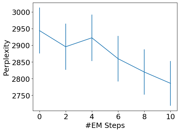
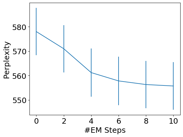
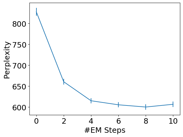
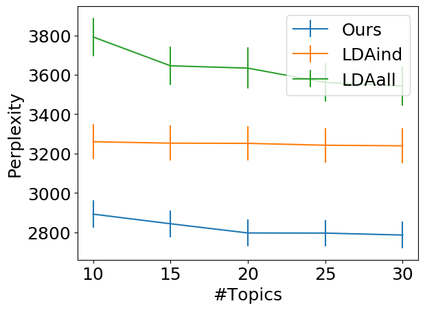
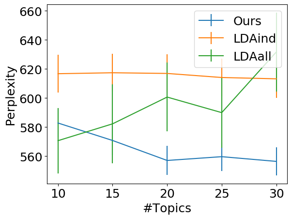
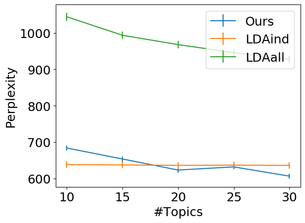
Figure 3 shows the test perplexity of the proposed method with different numbers of EM steps. As the number of the EM steps increased, the perplexity decreased. Figure 4 shows the test perplexity with different numbers of topics attained by the proposed method, LDAind, and LDAall. Particularly when the number of topics was not small, the proposed method achieved better performance than LDA. Table 3 shows the training time as achieved by computers with a 2.60GHz CPU. Since the proposed method needs to be trained by randomly sampling support and query data, its training time was long, but not so different from that of LDAall. The computation time of the proposed method in the test phase was 0.21, 0.03, and 0.08 seconds for the 20News, Digg, and NeurIPS data sets, respectively. The test time was short since the prior was obtained by feeding to the trained neural networks, and the EM steps are needed for only a few documents. Table 4 shows the estimated topics in the 20News data set. Related vocabulary terms that were specific to the corpus were appropriately clustered.

5 Conclusion

We proposed a few-shot learning method that can learn a topic model from just a small number of documents. The proposed method uses neural networks to output Dirichlet prior parameters for topic models. The neural networks are trained such that the topic model performs well when its parameters are estimated by maximizing the posterior probability based on the EM algorithm. We empirically demonstrated that the proposed method achieves better perplexity than existing topic model parameter estimation methods, and meta-learning methods. In future work, we will use our few-shot learning approach with the EM layers and prior distribution generating neural networks for other models, such as Gaussian mixtures, and non-negative matrix factorization.

References

- [1] A. Acharya, A. Rawal, R. J. Mooney, and E. R. Hruschka. Using both latent and supervised shared topics for multitask learning. In Joint European Conference on Machine Learning and Knowledge Discovery in Databases, pages 369–384. Springer, 2013.
- [2] M. Andrychowicz, M. Denil, S. Gomez, M. W. Hoffman, D. Pfau, T. Schaul, B. Shillingford, and N. De Freitas. Learning to learn by gradient descent by gradient descent. In Advances in Neural Information Processing Systems, pages 3981–3989, 2016.
- [3] S. Bartunov and D. Vetrov. Few-shot generative modelling with generative matching networks. In International Conference on Artificial Intelligence and Statistics, pages 670–678, 2018.
- [4] Y. Bengio, S. Bengio, and J. Cloutier. Learning a synaptic learning rule. In International Joint Conference on Neural Networks, 1991.
- [5] L. Bertinetto, J. F. Henriques, P. H. Torr, and A. Vedaldi. Meta-learning with differentiable closed-form solvers. In International Conference on Learning Representations, 2019.
- [6] D. M. Blei. Probabilistic topic models. Communications of the ACM, 55(4):77–84, 2012.
- [7] D. M. Blei and J. D. Lafferty. Dynamic topic models. In International Conference on Machine Learning, pages 113–120, 2006.
- [8] D. M. Blei, A. Y. Ng, and M. I. Jordan. Latent Dirichlet allocation. Journal of Machine Learning Research, 3(Jan):993–1022, 2003.
- [9] J. Bornschein, A. Mnih, D. Zoran, and D. J. Rezende. Variational memory addressing in generative models. In Advances in Neural Information Processing Systems, pages 3920–3929, 2017.
- [10] J. Boyd-Graber, Y. Hu, D. Mimno, et al. Applications of topic models. Foundations and Trends® in Information Retrieval, 11(2-3):143–296, 2017.
- [11] J. Chang, S. Gerrish, C. Wang, J. L. Boyd-Graber, and D. M. Blei. Reading tea leaves: How humans interpret topic models. In Advances in Neural Information Processing Systems, pages 288–296, 2009.
- [12] A. P. Dempster, N. M. Laird, and D. B. Rubin. Maximum likelihood from incomplete data via the em algorithm. Journal of the Royal Statistical Society: Series B, 39(1):1–22, 1977.
- [13] G. Doyle and C. Elkan. Accounting for burstiness in topic models. In International Conference on Machine Learning, pages 281–288, 2009.
- [14] H. Edwards and A. Storkey. Towards a neural statistician. arXiv preprint arXiv:1606.02185, 2016.
- [15] A. Faisal, J. Gillberg, J. Peltonen, G. Leen, and S. Kaski. Sparse nonparametric topic model for transfer learning. In ESANN, 2012.
- [16] C. Finn, P. Abbeel, and S. Levine. Model-agnostic meta-learning for fast adaptation of deep networks. In International Conference on Machine Learning, pages 1126–1135, 2017.
- [17] C. Finn, K. Xu, and S. Levine. Probabilistic model-agnostic meta-learning. In Advances in Neural Information Processing Systems, pages 9516–9527, 2018.
- [18] M. Garnelo, D. Rosenbaum, C. Maddison, T. Ramalho, D. Saxton, M. Shanahan, Y. W. Teh, D. Rezende, and S. A. Eslami. Conditional neural processes. In International Conference on Machine Learning, pages 1690–1699, 2018.
- [19] T. L. Griffiths and M. Steyvers. Finding scientific topics. Proceedings of the National academy of Sciences, 101(suppl 1):5228–5235, 2004.
- [20] P. Gupta, Y. Chaudhary, T. Runkler, and H. Schütze. Neural topic modeling with continual lifelong learning. In International Conference on Machine Learning, 2020.
- [21] L. B. Hewitt, M. I. Nye, A. Gane, T. Jaakkola, and J. B. Tenenbaum. The variational homoencoder: Learning to learn high capacity generative models from few examples. arXiv preprint arXiv:1807.08919, 2018.
- [22] T. Hofmann. Probabilistic latent semantic analysis. In Conference on Uncertainty in Artificial Intelligence, pages 289–296, 1999.
- [23] T. Hofmann. Collaborative filtering via Gaussian probabilistic latent semantic analysis. In Annual International ACM SIGIR Conference on Research and Development in Informaion Retrieval, pages 259–266, 2003.
- [24] K. Hsu, S. Levine, and C. Finn. Unsupervised learning via meta-learning. In International Conference on Learning Representations, 2018.
- [25] C. Hu, P. Rai, and L. Carin. Transfer learning for hierarchically supervised topic models. In NIPS Workshop in Transfer and Multi-task Learning, 2015.
- [26] T. Iwata and A. Kumagai. Meta-learning from tasks with heterogeneous attribute spaces. Advances in Neural Information Processing Systems, 33, 2020.
- [27] T. Iwata, S. Watanabe, T. Yamada, and N. Ueda. Topic tracking model for analyzing consumer purchase behavior. In International Joint Conference on Artificial Intelligence, 2009.
- [28] T. Iwata, T. Yamada, and N. Ueda. Probabilistic latent semantic visualization: topic model for visualizing documents. In ACM SIGKDD International Conference on Knowledge Discovery and Data Mining, pages 363–371, 2008.
- [29] J.-H. Kang, J. Ma, and Y. Liu. Transfer topic modeling with ease and scalability. In SIAM International Conference on Data Mining, pages 564–575, 2012.
- [30] S. S. Kataria, K. S. Kumar, R. R. Rastogi, P. Sen, and S. H. Sengamedu. Entity disambiguation with hierarchical topic models. In ACM SIGKDD International Conference on Knowledge Discovery and Data Mining, pages 1037–1045, 2011.
- [31] H. Kim, A. Mnih, J. Schwarz, M. Garnelo, A. Eslami, D. Rosenbaum, O. Vinyals, and Y. W. Teh. Attentive neural processes. In International Conference on Learning Representations, 2019.
- [32] H.-U. Kim, Y. J. Koh, and C.-S. Kim. Meta learning for unsupervised clustering. In BMVC, page 249, 2019.
- [33] T. Kim, J. Yoon, O. Dia, S. Kim, Y. Bengio, and S. Ahn. Bayesian model-agnostic meta-learning. In Advances in Neural Information Processing Systems, 2018.
- [34] D. P. Kingma and J. Ba. Adam: A method for stochastic optimization. In International Conference on Learning Representations, 2015.
- [35] B. M. Lake. Compositional generalization through meta sequence-to-sequence learning. In Advances in Neural Information Processing Systems, pages 9788–9798, 2019.
- [36] K. Lang. Newsweeder: learning to filter netnews. In International Conference on Machine Learning, pages 331–339, 1995.
- [37] D. Li, J. Zhang, Y. Yang, C. Liu, Y.-Z. Song, and T. M. Hospedales. Episodic training for domain generalization. In IEEE International Conference on Computer Vision, pages 1446–1455, 2019.
- [38] Z. Li, F. Zhou, F. Chen, and H. Li. Meta-SGD: Learning to learn quickly for few-shot learning. arXiv preprint arXiv:1707.09835, 2017.
- [39] T. Lin, W. Tian, Q. Mei, and H. Cheng. The dual-sparse topic model: mining focused topics and focused terms in short text. In International Conference on World Wide Web, pages 539–550, 2014.
- [40] J. D. Mcauliffe and D. M. Blei. Supervised topic models. In Advances in Neural Information Processing Systems, pages 121–128, 2008.
- [41] D. Mimno and D. Blei. Bayesian checking for topic models. In Conference on Empirical Methods in Natural Language Processing, pages 227–237, 2011.
- [42] T. Minka. Estimating a Dirichlet distribution, 2000.
- [43] J. Narwariya, P. Malhotra, L. Vig, G. Shroff, and T. Vishnu. Meta-learning for few-shot time series classification. In ACM IKDD CoDS and COMAD, pages 28–36. 2020.
- [44] A. Paszke, S. Gross, S. Chintala, G. Chanan, E. Yang, Z. DeVito, Z. Lin, A. Desmaison, L. Antiga, and A. Lerer. Automatic differentiation in PyTorch. In Neural Information Processing Systems Autodiff Workshop, 2017.
- [45] S. Ravi and H. Larochelle. Optimization as a model for few-shot learning. In International Conference on Learning Representations, 2017.
- [46] S. Reed, Y. Chen, T. Paine, A. van den Oord, S. A. Eslami, D. Rezende, O. Vinyals, and N. de Freitas. Few-shot autoregressive density estimation: Towards learning to learn distributions. In International Conference on Learning Representations, 2018.
- [47] D. J. Rezende, S. Mohamed, I. Danihelka, K. Gregor, and D. Wierstra. One-shot generalization in deep generative models. In Proceedings of the 33rd International Conference on International Conference on Machine Learning, pages 1521–1529, 2016.
- [48] A. A. Rusu, D. Rao, J. Sygnowski, O. Vinyals, R. Pascanu, S. Osindero, and R. Hadsell. Meta-learning with latent embedding optimization. In International Conference on Learning Representations, 2019.
- [49] A. Santoro, S. Bartunov, M. Botvinick, D. Wierstra, and T. Lillicrap. Meta-learning with memory-augmented neural networks. In International Conference on Machine Learning, pages 1842–1850, 2016.
- [50] J. Schmidhuber. Evolutionary principles in self-referential learning. on learning now to learn: The meta-meta-meta…-hook. Master’s thesis, Technische Universitat Munchen, Germany, 1987.
- [51] J. Snell, K. Swersky, and R. Zemel. Prototypical networks for few-shot learning. In Advances in Neural Information Processing Systems, pages 4077–4087, 2017.
- [52] N. Srivastava, G. Hinton, A. Krizhevsky, I. Sutskever, and R. Salakhutdinov. Dropout: a simple way to prevent neural networks from overfitting. Journal of Machine Learning Research, 15(1):1929–1958, 2014.
- [53] W. Tang, L. Liu, and G. Long. Few-shot time-series classification with dual interpretability. In ICML Time Series Workshop. 2019.
- [54] O. Vinyals, C. Blundell, T. Lillicrap, D. Wierstra, et al. Matching networks for one shot learning. In Advances in Neural Information Processing Systems, pages 3630–3638, 2016.
- [55] Y. Xie, H. Jiang, F. Liu, T. Zhao, and H. Zha. Meta learning with relational information for short sequences. In Advances in Neural Information Processing Systems, pages 9901–9912, 2019.
- [56] J. Xu, J.-F. Ton, H. Kim, A. R. Kosiorek, and Y. W. Teh. Metafun: Meta-learning with iterative functional updates. In International Conference on Machine Learning, 2020.
- [57] H. Yao, Y. Wei, J. Huang, and Z. Li. Hierarchically structured meta-learning. In International Conference on Machine Learning, pages 7045–7054, 2019.
- [58] M. Zaheer, S. Kottur, S. Ravanbakhsh, B. Poczos, R. R. Salakhutdinov, and A. J. Smola. Deep sets. In Advances in Neural Information Processing Systems, pages 3391–3401, 2017.
- [59] W. X. Zhao, J. Jiang, J. Weng, J. He, E.-P. Lim, H. Yan, and X. Li. Comparing twitter and traditional media using topic models. In European Conference on Information Retrieval, pages 338–349. Springer, 2011.
- [60] Y. Zuo, J. Zhao, and K. Xu. Word network topic model: a simple but general solution for short and imbalanced texts. Knowledge and Information Systems, 48(2):379–398, 2016.