On the Complexity of Inverse Mixed Integer Linear Optimization

Abstract

Inverse optimization is the problem of determining the values of missing input parameters for an associated forward problem that are closest to given estimates and that will make a given target vector optimal. This study is concerned with the relationship of a particular inverse mixed integer linear optimization problem (MILP) to both the forward problem and the separation problem associated with its feasible region. We show that a decision version of the inverse MILP in which a primal bound is verified is ${\mathsf{coNP}}$–complete, whereas primal bound verification for the associated forward problem is ${\mathsf{NP}}$–complete, and that the optimal value verification problems for both the inverse problem and the associated forward problem are complete for the complexity class ${\mathsf{D}}^{{\mathsf{P}}}$. We also describe a cutting-plane algorithm for solving inverse MILPs that illustrates the close relationship between the separation problem for the convex hull of solutions to a given MILP and the associated inverse problem. The inverse problem is shown to be equivalent to the separation problem for the radial cone defined by all inequalities that are both valid for the convex hull of solutions to the forward problem and binding at the target vector. Thus, the inverse, forward, and separation problems can be said to be equivalent.

Keywords: Inverse optimization, mixed integer linear optimization, computational complexity, polynomial hierarchy

1 Introduction

In this paper, we study the relationship of the inverse integer linear optimization problem to both the optimization problem from which it arose, which we refer to as the forward problem, and the associated separation problem. We show that these three problems have a strong relationship from an algorithmic standpoint by describing a cutting-plane algorithm for the inverse problem that uses the forward problem as an oracle and also solves the separation problem. From a complexity standpoint, we show that certain decision versions of these three problems are all complete for the complexity class ${\mathsf{D}}^{{\mathsf{P}}}$, introduced originally by Papadimitriou and Yannakakis (1982). Motivated by this analysis, we argue that the optimal value verification problem is a more natural decision problem to associate with many optimization problems and that ${\mathsf{D}}^{{\mathsf{P}}}$ may provide a more appropriate class in which to place difficult discrete optimization problems than the more commonly cited ${\mathsf{NP}}$-hard.

An optimization problem is that of determining a member of a feasible set (an optimal solution) that minimizes the value of a given objective function. The feasible set is typically described as the points in a vector space satisfying a given set of equations, inequalities, and disjunctions (usually in the form of a requirement that the value of a certain element of the solution take on values in a discrete set).

An inverse optimization problem, in contrast, is a related problem in which the description of the original forward optimization problem is incomplete (some parameters are missing or cannot be observed), but a full or partial solution can be observed. The goal is to determine values for the missing parameters with respect to which the given solution would be optimal for the resulting complete problem. Estimates for the missing parameters may be given, in which case the goal is to produce a set of parameters that is as close to the given estimates as possible by some metric.

The forward optimization problem of interest in this paper is the mixed integer linear optimization problem

$$\max_{x\in\mathcal{S}}d^{\top}x,$$ (MILP)

where $d\in\mathbb{Q}^{n}$ and

$$\mathcal{S}=\left\{x\in\mathbb{R}^{n}\;\middle|\;Ax\leq b\right\}\cap(\mathbb{Z}^{r}\times\mathbb{R}^{n-r})$$

for $A\in\mathbb{Q}^{m\times n}$, $b\in\mathbb{Q}^{m}$ and for some nonnegative integer $r$. In the case when $r=0$, (MILP) is known simply as a linear optimization problem (LP).

One can associate a number of different inverse problems with (MILP), depending on what parts of the description $(A,b,d)$ are unknown and what form the objective function of the inverse problem takes. Here, we study the case in which the objective function $d$ of the forward problem is the unknown element of the input, but in which $A$ and $b$, along with a target vector $x^{0}\in\mathbb{Q}^{n}$, are given. A feasible solution to the inverse problem (which we refer to as a feasible objective) is any $\hat{d}\in\mathbb{R}^{n}$ for which $\hat{d}^{\top}x^{0}=\max_{x\in\mathcal{S}}\hat{d}^{\top}x$.

It is important in the analysis that follows to be precise about the assumptions on the target vector $x^{0}$. Our initial informal statement of the problem implicitly assumed that $x^{0}\in\mathcal{S}$, since otherwise, $x^{0}$ cannot technically be an optimal solution, regardless of the objective function chosen. On the other hand, neither the more precise mathematical definition given in the preceding paragraph nor the mathematical formulations we introduce shortly require $x^{0}\in\mathcal{S}$ and both can be interpreted even when $x^{0}\not\in\mathcal{S}$. As a practical matter when solving inverse problems in practice, this subtle distinction is usually not very important, since membership in $\mathcal{S}$ can be verified in a preprocessing step if necessary. However, in the context of complexity analysis and in considering the relationship of the inverse problem to the related separation and optimization problems, this point is important and we return to it. For example, if we do not make this assumption, the inverse optimization problem can be seen to be equivalent to both the separation problem and the problem of verifying a given dual bound on the optimal solution value of an MILP.

For these and other reasons that will become clear, we do not assume $x^{0}\in\mathcal{S}$, but this may make some aspects of what follows a bit ambiguous. To resolve any ambiguity, we replace $\mathcal{S}$ with the augmented set $\mathcal{S}^{+}=\mathcal{S}\cup\{x^{0}\}$, when appropriate, in the remainder of the paper.

1.1 Formulations

We now present several mathematical formulations of what we refer to from now on as the inverse mixed integer linear optimization problem (IMILP). A straightforward formulation of this problem that explains why we refer to the general class of problems as “inverse” problems is as that of computing the mathematical inverse of a function that is parametric in some part of the input to a given problem instance. In this case, the relevant function is

$$\phi(d)=\operatorname{argmax}_{x\in\mathcal{S}^{+}}d^{\top}x.$$

In terms of the function $\phi$, a feasible objective is any element of the preimage $\phi^{-1}(x^{0})$. To make the IMILP an optimization problem in itself, we add an objective function $f:\mathbb{Q}^{n}\rightarrow\mathbb{Q}$, to obtain the general formulation

$$\min_{d\in\phi^{-1}(x^{0})}f(d).$$ (INV)

The traditional objective function used for inverse problems in the literature is $f(d):=\|c-d\|$, the minimum norm distance from $d$ to a given estimated objective function $c\in\mathbb{Q}^{n}$ (the specific norm is not important for defining the problem, but we assume a $p$-norm when proving the formal results). This choice of objective, although standard, has some nonintuitive properties. First, it is not scale-invariant—scaling a given feasible objective $\hat{d}$ changes the resulting objective function value. In other words, $f(\hat{d})\not=f(\lambda\hat{d})$ for $\lambda\not=1$, so $\hat{d}$ and $\lambda\hat{d}$ do not have the same objective function value, although it is clear that $\hat{d}$ and $\lambda\hat{d}$ are equivalent solutions in most settings. Second, the objective function value is always nonnegative. Both these properties have implications we discuss further below.

The formulation (INV) does not suggest any direct connection to existing methodology for solving mathematical optimization problems, so we next discuss several alternative formulations of the problem as a standard mathematical optimization problem. We first consider the following formulation of the IMILP as the semi-infinite optimization problem

$$\min_{d} \|c-d\|,$$ (IMILP)

$$\operatorname{s.\!t.} d^{\top}x\leq d^{\top}x^{0} \forall x\in\mathcal{S}.$$

As in the first formulation, $d$ is a vector of variables, while $c\in\mathbb{Q}^{n}$ is the given estimated objective function. Note that in (IMILP), if we instead let $x^{0}$ vary, replacing it with a variable $x$, and interpret $d$ as a fixed objective function, replacing $\|c-d\|$ with the objective $d^{\top}x$ of the forward problem (MILP), we get a reformulation of the forward problem (MILP) itself. This formulation can be made finite, in the case that $\mathcal{S}$ is bounded, by replacing the possibly infinite set of inequalities with only those corresponding to the extreme points of $\operatorname{conv}(\mathcal{S})$. In the unbounded case, we also need to include inequalities corresponding to the extreme rays.

Problem (IMILP) can also be formulated as a conic optimization problem. Although this is not the traditional way of describing the problem mathematically, it is arguably the most intuitive representation and is the one that best highlights the underlying mathematical structure. The following cones and related sets all play important roles in what follows:

$$\mathcal{K}:=\{(y,d)\in\mathbb{R}^{n+1}\mid\|c-d\|\leq y\},$$

$$\mathcal{K}(\gamma):=\{d\in\mathbb{R}^{n}\mid(\gamma,d)\in\mathcal{K}\},$$

$$\mathcal{K}^{*}(\gamma):=\{x\in\mathbb{R}^{n}\,\mid\,d^{\top}(x^{0}-x)\leq 0\;\forall d\in\mathcal{K}(\gamma)\},$$

$$\mathcal{C}(x^{0}):=\operatorname{cone}(\mathcal{S}^{+}-\{x^{0}\})=\operatorname{cone}(\{x-x^{0}\mid x\in\mathcal{S}\}),\textrm{ and}$$

$$\mathcal{C}^{\circ}(x^{0}):=\{d\in\mathbb{R}^{n}\mid d^{\top}(x-x^{0})\leq 0\;\forall x\in\mathcal{S}\}.$$

Here, $\mathcal{K}$ is a norm cone, while $\mathcal{K}(\gamma)$ is a ball with center $c$ and radius $\gamma$ that is a level set of $\mathcal{K}$ and contains vectors whose objective value in (IMILP) is at most $\gamma$. $\mathcal{K}^{*}(\gamma)$ is the set consisting of points, not necessarily in $\mathcal{S}$, that have an objective function value greater than or equal to that of $x^{0}$ for all the vectors in $\mathcal{K}(\gamma)$. $\mathcal{K}^{*}(\gamma)$ can also be seen as the radial cone obtained by translating the dual of $\operatorname{cone}(\mathcal{K}(\gamma))$ from the origin to $x^{0}$ (this is the reason for the slightly abused notation that is typically used to denote the dual of a cone).

The set $\mathcal{C}^{\circ}(x^{0})$ is the set of feasible objectives of (IMILP) with target vector $x^{0}$ and is precisely the polar of $\mathcal{C}(x^{0})$. $\mathcal{C}(x^{0})$, on the other hand, is a translation to the origin of the radial cone that is the intersection of the half-spaces associated with the facet-defining inequalities valid for $\operatorname{conv}(\mathcal{S}^{+})$ that are binding at $x^{0}$. Equivalently, it is the radial cone with vertex at $x^{0}$ generated by rays $x-x^{0}$ for all $x\in S$. The notational dependence on $x^{0}$ in both sets is for convenience later when various target vectors will be constructed in the reductions used in the complexity proofs. We should also point out that $\mathcal{C}^{\circ}(x^{0})$ is referred to as the normal cone at $x^{0}$ in convex analysis and would be denoted as $N_{\operatorname{conv}(\mathcal{S}^{+})}(x^{0})$ in the standard notation (Rockafellar, 1970). Due to the obvious connections with the theory of polarity in discrete optimization, however, we maintain our alternative notation here.

Finally, in terms of the cones and sets introduced, (IMILP) can be reformulated as

$$\min_{d\in\mathcal{K}(y)\cap\mathcal{C}^{\circ}(x^{0})}y.$$ (IMILP-C)

Figure 1 illustrates the geometry of the inverse MILP. Here, $\mathcal{S}$ is the discrete set indicated by the black dots. The estimated objective function is $c=(0,2)$ and the target vector is $x^{0}=(3,1)$. The convex hull of $\mathcal{S}$ and the cone $\mathcal{C}^{\circ}(x^{0})$ (translated to $x^{0}$) are shaded. The ellipsoids show the sets of points with a fixed distance to $x^{0}+c$ for a given norm. The (unique) optimal solution for this example is vector $d^{*}$, which is also the unique point of intersection of $\mathcal{K}(\|c-d^{*}\|)$ and $\mathcal{C}^{\circ}(x^{0})$. The point $x^{0}+d^{*}$ is also illustrated.

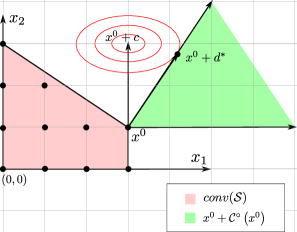
Figure 1: Two-dimensional inverse MILP

Figure 2 presents a more detailed picture of how the various cones and sets introduced so far are related by displaying sets $\operatorname{conv}(\mathcal{S})$, $\mathcal{C}^{\circ}(x^{0})$, $\operatorname{cone}(\mathcal{K}(\gamma))$, and $\mathcal{K}^{*}(\gamma)$ for four different two-dimensional inverse problems with Euclidean norm.

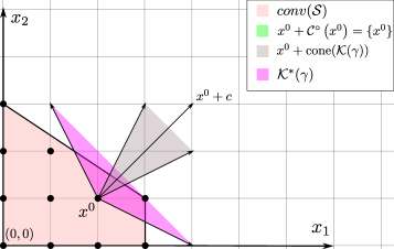
(a) Instance 1

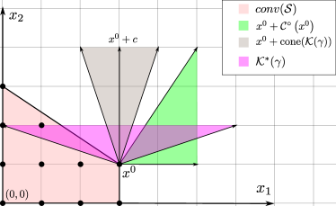
(b) Instance 2

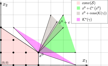
(c) Instance 3

(d) Instance 4

Figure 2: Pictorial illustration of sets $\operatorname{conv}(\mathcal{S})$, $\mathcal{C}^{\circ}(x^{0})$, $\mathcal{K}(\gamma)$, $\mathcal{K}^{*}(\gamma)$ for 4 IMILP instances

Notions of duality that underlie many of the concepts discussed in the paper can be seen in the relationships between these sets. $\mathcal{K}^{*}(\gamma)$ and $\mathcal{S}$ can be thought of as being in the “primal space” with respect to the original problem (the space of primal solutions), whereas the cone $\mathcal{C}^{\circ}(x^{0})$ and the ball $\mathcal{K}(\gamma)$ can be thought of as being in the “dual space,” the space of directions. In the context of the inverse problem, these roles are reversed, e.g., $\mathcal{C}^{\circ}(x^{0})$ is the set of primal solutions for the inverse problem.

The interpretation of the feasible region of (IMILP) as the polar of $\mathcal{C}(x^{0})$ leads to a third formulation in terms of the so-called $1$-polar of $\operatorname{conv}(\mathcal{S})$, defined as

$$\mathcal{P}^{1}=\{d\in\mathbb{R}^{n}\mid d^{\top}x\leq 1\;\forall x\in\operatorname{conv}(\mathcal{S})\}.$$

When $\operatorname{conv}(\mathcal{S})$ is full-dimensional and $0\in\operatorname{int}\left(\operatorname{conv}(\mathcal{S})\right)$, the 1-polar is the set of all normalized inequalities valid for $\operatorname{conv}(\mathcal{S})$ (see (Schrijver, 1986) for definitions). Under these assumptions, (IMILP) can also be reformulated as

$$\min_{d,\rho} \|c-\rho d\|$$

$$\operatorname{s.\!t.} d\in\mathcal{P}^{1},$$

$$d^{\top}x^{0}\geq 1,$$ (IMILP-1P)

$$\rho\geq 0.$$

In (1.1), $\rho$ is a multiplier that allows for scaling of the members of the 1-polar (which are normalized) in order to improve the objective function value, but otherwise plays no important role. It would seem to be more natural to require $\|c\|=1$ or normalize in some other way to avoid this scaling, but the presence of this scaling variable highlights that the usual formulation does have this rather unnatural feature. When $d\in\mathcal{P}^{1}$, the single constraint $d^{\top}x^{0}\geq 1$ is, in effect, equivalent to the exponential set of constraints in (IMILP), and ensures $d$ is a feasible objective. Observe also that relaxing the constraint $d^{\top}x^{0}\geq 1$ yields a problem similar to the classical separation problem, but with a different objective function. We revisit this idea in Section 2.

Note that when $\operatorname{conv}(\mathcal{S}^{+})$ is not full-dimensional, any objective vector in the subspace orthogonal to the affine space containing $\operatorname{conv}(\mathcal{S}^{+})$ is a feasible objective for the inverse problem. If we let $c_{\mathcal{S}^{+}}$ be the projection of $c$ onto the smallest affine space that contains $\mathcal{S}^{+}$ and $c_{\mathcal{S}^{+}}^{\perp}$ be the projection of $c$ onto the orthogonal subspace, so that $c=c_{\mathcal{S}^{+}}+c_{\mathcal{S}^{+}}^{\perp}$, then whenever $x^{0}$ is in the relative interior of $\operatorname{conv}(\mathcal{S})$, $c_{\mathcal{S}}^{\perp}$ will be an optimal solution. On the other hand, when $\operatorname{conv}(\mathcal{S})$ is full-dimensional, the unique optimal solution is 0 whenever $x^{0}$ is in the interior of $\operatorname{conv}(\mathcal{S})$.

1.2 The Separation Problem

The close relationship between the inverse problem (IMILP) and the separation problem for $\operatorname{conv}(\mathcal{S})$ should already be evident, but we now introduce this idea formally. Given an $\hat{x}\in\mathbb{Q}^{n}$, the separation problem for $\operatorname{conv}(\mathcal{S})$ is to determine whether $\hat{x}\in\operatorname{conv}(\mathcal{S})$ and, if not, to generate a hyperplane separating $\hat{x}$ from $\operatorname{conv}(\mathcal{S})$. When $\hat{x}\not\in\operatorname{conv}(\mathcal{S})$ and such a separating hyperplane exists, we can associate with each such hyperplane a valid inequality, defined as follows.

Definition 1.

A valid inequality for a set $\mathcal{Q}$ is a pair $(a,b)\in\mathbb{Q}^{n+1}$ such that $\mathcal{Q}\subseteq\{x\in\mathbb{R}^{n}\mid a^{\top}x\leq b\}$. The inequality is said to be violated by $\hat{x}\in\mathbb{Q}^{n}$ if $a^{\top}\hat{x}>b$.

Generating a separating hyperplane is equivalent to determining the existence of $\hat{d}\in\mathbb{R}^{n}$ such that

$${\hat{d}}^{\top}\hat{x}>{\hat{d}}^{\top}x\quad\forall x\in\mathcal{S}.$$

In such a case, $({\hat{d}}^{\top},\max_{x\in\mathcal{S}}{\hat{d}}^{\top}x)$ is an inequality valid for $\operatorname{conv}(\mathcal{S})$ that is violated by $\hat{x}$ (therefore proving that $\hat{x}\not\in\operatorname{conv}(\mathcal{S})$). On the other hand, $\hat{d}$ is feasible for (IMILP) if and only if

$${\hat{d}}^{\top}x\leq{\hat{d}}^{\top}x^{0}\quad\forall x\in\mathcal{S},$$

which similarly means that $({\hat{d}}^{\top},{\hat{d}}^{\top}x^{0})$ is an inequality valid for $\operatorname{conv}(\mathcal{S})$. Thus, feasible solutions to (IMILP) can also be viewed as an inequality valid for $\operatorname{conv}(\mathcal{S})$ binding at $x^{0}$. Moreover, when $x^{0}\not\in\operatorname{conv}(\mathcal{S})$, $({\hat{d}}^{\top},\max_{x\in\mathcal{S}}{\hat{d}}^{\top}x)$ is an inequality valid for $\operatorname{conv}(\mathcal{S})$ that is violated by $x^{0}$. This provides an informal argument for the equivalence of (IMILP) and the separation problem. More will be said about this in the following sections.

1.3 Previous Work

There are a range of different flavors of the inverse optimization problem. The inverse problem we investigate is to determine objective function coefficients that make a given solution optimal, but other flavors of inverse optimization include constructing a missing part of either the coefficient matrix or the right-hand sides. Heuberger (2004) provides a detailed survey of different types of inverse combinatorial optimization problems, including types for which the inverse problem seeks parameters other than objective function coefficients. A survey of solution procedures for specific combinatorial problems is provided, as well as a classification of the inverse problems that are common in the literature. According to this classification, the inverse problem we study in this paper is an unconstrained, single feasible objective, and unit weight norm inverse problem. Our results can be straightforwardly extended to some related cases, such as multiple given solutions.

Cai et al. (1999) examine an inverse center location problem in which the aim is to construct part of the coefficient matrix that minimizes the distances between nodes for a given solution. It is shown that even though the center location problem is polynomially solvable, this particular inverse problem is ${\mathsf{NP}}$-hard. This is done by way of a polynomial transformation of the satisfiability problem to the decision version of the inverse center location problem. This analysis indicates that the problem of constructing part of the coefficient matrix is harder than the forward version of the problem.

Huang (2005) examines the inverse knapsack problem and inverse integer optimization problems. Pseudopolynomial algorithms for both the inverse knapsack problem and inverse problems for which the forward problem has a fixed number of constraints are presented. The latter is achieved by transforming the inverse problem to a shortest path problem on a directed graph.

Schaefer (2009) studies general inverse integer optimization problems. Using super-additive duality, a polyhedral description of the set of all feasible objective functions is derived. This description has only continuous variables but an exponential number of constraints. A solution method using this polyhedral description is proposed. Finally, Wang (2009) suggests a cutting-plane algorithm similar to the one suggested below and presents computational results on several test problems with an implementation of this algorithm.

The case when the feasible set is an explicitly described polyhedron is well-studied by Ahuja and Orlin (2001). In their study, they analyze the shortest path, assignment, minimum cut, and minimum cost flow problems under the $\ell_{1}$ and $\ell_{\infty}$ norms in detail. They also conclude that the inverse optimization problem is polynomially solvable when the forward problem is polynomially solvable. The present study aims to generalize the result of Ahuja and Orlin to the case when the forward problem is not necessarily polynomially solvable, as well as to make connections to other well-known problems.

In the remainder of the paper, we first introduce a cutting-plane algorithm for solving (IMILP) in the case of the $\ell_{\infty}$ and $\ell_{1}$ norms. In Section 2, we show that for these norms, the problem can be expressed as an LP using standard techniques, albeit one with an exponential number of constraints. The reformulation can then be readily solved using a standard cutting-plane approach, as observed by Wang (2009). On the other hand, in Section 4, we establish the computational complexity of the problem and show that it is the same for any $p$-norm.

2 A Cutting-plane Algorithm

In this section, we describe a basic cutting-plane algorithm for solving (IMILP) under the $\ell_{1}$ and $\ell_{\infty}$ norms. The algorithm is conceptual in nature and presented in order to illustrate the relationship of the inverse problem to both the forward problem and the separation problem. A practical implementation of this algorithm would require additional sophistication and the development of such an implementation is not our goal in this paper.

The first step in the algorithm is to formulate (IMILP) explicitly as an LP using standard linearization techniques. The objective function of the inverse MILP under the $\ell_{1}$ norm can be linearized by the introduction of variable vector $y$, and associated constraints as shown below.

$$z_{1}^{-1}=\min_{d,y,\theta} \quad\theta$$

$$\operatorname{s.\!t.} \quad\theta=\sum_{i=1}^{n}{y_{i}},$$ (0a)

$$\quad c_{i}-d_{i}\leq y_{i} \forall i\in\{1,2,\dots,n\},$$ (0b)

$$\quad d_{i}-c_{i}\leq y_{i} \forall i\in\{1,2,\dots,n\},$$ (0c)

$$\quad d^{\top}x\leq d^{\top}x^{0} \forall x\in\mathcal{S}.$$ (0d)

For the case of the $\ell_{\infty}$ norm, the variable $\theta$ and two sets of constraints are introduced to linearize the problem.

$$z_{\infty}^{-1}=\min_{d,\theta} \quad\theta$$

$$\operatorname{s.\!t.} \quad c_{i}-d_{i}\leq\theta \forall i\in\{1,2,\dots,n\},$$ (0a)

$$\quad d_{i}-c_{i}\leq\theta \forall i\in\{1,2,\dots,n\},$$ (0b)

$$\quad d^{\top}x\leq d^{\top}x^{0} \forall x\in\mathcal{S}.$$ (0c)

Both ( ‣ 2) and ( ‣ 2) are continuous, semi-infinite optimization problems. To obtain a finite problem, one can replace the inequalities (0d) and (0c) with constraints (1) and (2) involving the finite set $\mathcal{E}$ of extreme points and $\mathcal{R}$ of rays of the convex hull of $\mathcal{S}$.

$$d^{\top}x \leq d^{\top}x^{0} \forall x\in\mathcal{E},$$ (1)

$$d^{\top}r \leq 0 \forall r\in\mathcal{R}.$$ (2)

Although constraints (1) and (2) yield a finite formulation, the cardinality of $\mathcal{E}$ and $\mathcal{R}$ may still be very large and generating them explicitly is likely to be very challenging. It is thus not practical to construct this mathematical program explicitly via a priori enumeration. The cutting-plane algorithm avoids explicitly enumerating the inequalities in the formulation by generating them dynamically in the standard way. The algorithm described here is unsophisticated and although versions of it have appeared in the literature, we describe it again to illustrate the basic principles at work and to make the connection to a similar existing algorithm for solving the separation problem.

We describe the algorithm only for the case of ( ‣ 2), as the extension to ( ‣ 2) is straightforward. We assume $\mathcal{S}$ is bounded, so that $\operatorname{conv}(\mathcal{S})$ has no extreme rays and $\mathcal{R}=\emptyset$. As previously observed, ( ‣ 2) is an LP with an exponential class (0c) of inequalities. Nevertheless, the well-known result of Grötschel et al. (1993) tells us that ( ‣ 2) can be solved efficiently using a cutting-plane algorithm, provided we can solve the problem of separating a given point from the feasible region efficiently. The constraints (0a) and (0b) can be explicitly enumerated, so we focus on generation of constraints (0c), which means we are solving the separation problem for set $\mathcal{C}^{\circ}(x^{0})$. For an arbitrary $\hat{d}\in\mathbb{R}^{n}$, this separation problem is to either verify that $\hat{d}\in\mathcal{C}^{\circ}(x^{0})$ or determine a hyperplane separating $\hat{d}$ from $\mathcal{C}^{\circ}(x^{0})$.

The question of whether $\hat{d}\in\mathcal{C}^{\circ}(x^{0})$ is equivalent to asking whether $\hat{d}^{\top}x\leq\hat{d}^{\top}x^{0}$ for all $x\in\mathcal{S}$. This can be answered by determining $x^{*}\in\operatorname{argmax}_{x\in\mathcal{S}}\hat{d}^{\top}x$. When $\hat{d}^{\top}x^{*}>\hat{d}^{\top}x^{0}$, then $x^{*}$ yields a new inequality valid for $\mathcal{C}^{\circ}(x^{0})$ that is violated by $\hat{d}$. Otherwise, we have a proof that $\hat{d}\in\mathcal{C}^{\circ}(x^{0})$. Hence, the separation problem for $\mathcal{C}^{\circ}(x^{0})$ is equivalent to the forward problem.

The algorithm alternates between solving a master problem and the separation problem just described, as usual. The initial master problem is an LP obtained by relaxing the constraints (0c) in ( ‣ 2). After solving the master problem, we attempt to separate its solution from the set $\mathcal{C}^{\circ}(x^{0})$ and either add the violated inequality or terminate, as appropriate. More formally, the master problem is to determine

$$\left(d^{k},\theta^{k}\right)\in\operatorname{argmin}_{\left(d,\theta\right)} \quad\theta \mathcal{P}_{k}$$ (Inv)

$$\operatorname{s.\!t.} \quad c_{i}-d_{i}\leq\theta \forall i\in\{1,2,\dots,n\},$$

$$\quad d_{i}-c_{i}\leq\theta \forall i\in\{1,2,\dots,n\},$$

$$\quad d^{\top}x\leq d^{\top}x^{0} \forall x\in\mathcal{E}_{k-1}$$

and the separation problem is to determine

$$x^{k}\in\operatorname{argmax}_{x\in\mathcal{S}}d^{k\top}x. \mathcal{P}_{k}$$ ()

Here, $\mathcal{E}_{k}=\{x^{1},\dots,x^{k}\}$ are the points in $\mathcal{S}$ generated so far (which are generally assumed to be extreme points of $\operatorname{conv}(\mathcal{S})$, but need not be in general). (Inv$\mathcal{P}_{k}$) is a relaxation of ( ‣ 2) consisting of only the valid inequalities corresponding to point in $\mathcal{E}_{k}$. When ($\mathcal{P}_{k}$) is unbounded, then $x^{0}$ is in the relative interior of $\operatorname{conv}(\mathcal{S})$ and $d=c_{\mathcal{S}}^{\perp}$ is an optimal solution, as mentioned earlier. The overall procedure is given in Algorithm 1.

Algorithm 1 Cutting-plane algorithm for ( ‣ 2)

1:$k\leftarrow 0$, $\mathcal{E}^{1}\leftarrow\emptyset$.

2:do

3:     $k\leftarrow k+1$.

4:     Solve (Inv$\mathcal{P}_{k}$) to determine $d^{k},\theta^{k}$.

5:     Solve ($\mathcal{P}_{k}$) to determine $x^{k}$ or show that ($\mathcal{P}_{k}$) is unbounded.

6:     if ($\mathcal{P}_{k}$) unbounded then

7:         $\theta^{*}\leftarrow\left\|c\right\|_{\infty}$, $d^{*}\leftarrow 0$, STOP.

8:     end if

9:     $\mathcal{E}_{k+1}\leftarrow\mathcal{E}_{k}\cup\{x^{k}\}$.

10:while $d^{k\top}(x^{k}-x^{0})>0$

11:$\theta^{*}\leftarrow\left\|c-d^{k}\right\|_{\infty}$, $d^{*}\leftarrow d^{k}$, STOP.

To understand the nature of the algorithm, observe that in iteration $k$, the master problem is equivalent to an inverse problem in which $\mathcal{S}$ is replaced $\mathcal{E}_{k}$. Equivalently, we are replacing $\mathcal{C}^{\circ}(x^{0})$ with the restricted set $\mathcal{C}^{\circ}_{k}(x^{0})$, taken to be the polar of $\mathcal{C}_{k}(x^{0})=\operatorname{cone}(\mathcal{E}_{k}-\{x^{0}\})$. Each member of $\mathcal{S}$ generated corresponds to a member of $\mathcal{C}(x^{0})$, so that the final product of the algorithm is a (partial) description of $\mathcal{C}(x^{0})$ and hence a partial description of $\mathcal{C}^{\circ}(x^{0})$. This is analogous to the way in which a traditional cutting-plane algorithm for solving the original forward problem generates a partial description of $\operatorname{conv}(\mathcal{S})$ and highlights the underlying duality between the H-representation and the V-representation of a polyhedron (see section 3.3).

We illustrate by considering a small example. Let $c=(2,-1)$, $x^{0}=(0,3)$ and $\mathcal{S}$ be as in Figure 3, where both $x_{1}$ and $x_{2}$ are integer and $\operatorname{conv}(\mathcal{S})$ is shown. The values of $k$, $d^{k}$, and $x^{k}$ in iterations 1–3 are given in Table 1.

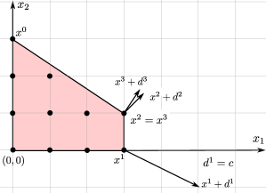
Figure 3: Feasible region and iterations of example problem

	$k$	$\mathcal{E}_{k}$	$d^{k}$	$x^{k}$	$\|c-d^{k}\|_{\infty}$
Initialization	$1$	$\emptyset$	$(2,-1)$	$(3,0)$	$0$
Iteration 1	$2$	$\{(3,0)\}$	$(0.5,0.5)$	$(3,1)$	$1.5$
Iteration 2	$3$	$\{(3,0),(3,1)\}$	$(0.4,0.6)$	$(3,1)$	$1.6$

Table 1: $k$, $d^{k}$, $x^{k}$, and $\mathcal{E}_{k}$ values through iterations

The (unique) optimal solution of this small example is $d^{3}=(0.4,0.6)$, and the optimal value is $\theta^{*}=\|c-d^{3}\|_{\infty}=1.6$.

Figure 4 provides a geometric visualization of another small example, illustrating how the algorithm would proceed when the set $\mathcal{S}$ is the collection of integer points inside the polyhedron marked in blue. Here, the cone $\mathcal{C}_{k}(x^{0})$ is explicitly shown and its expansion can be seen as generators are added.

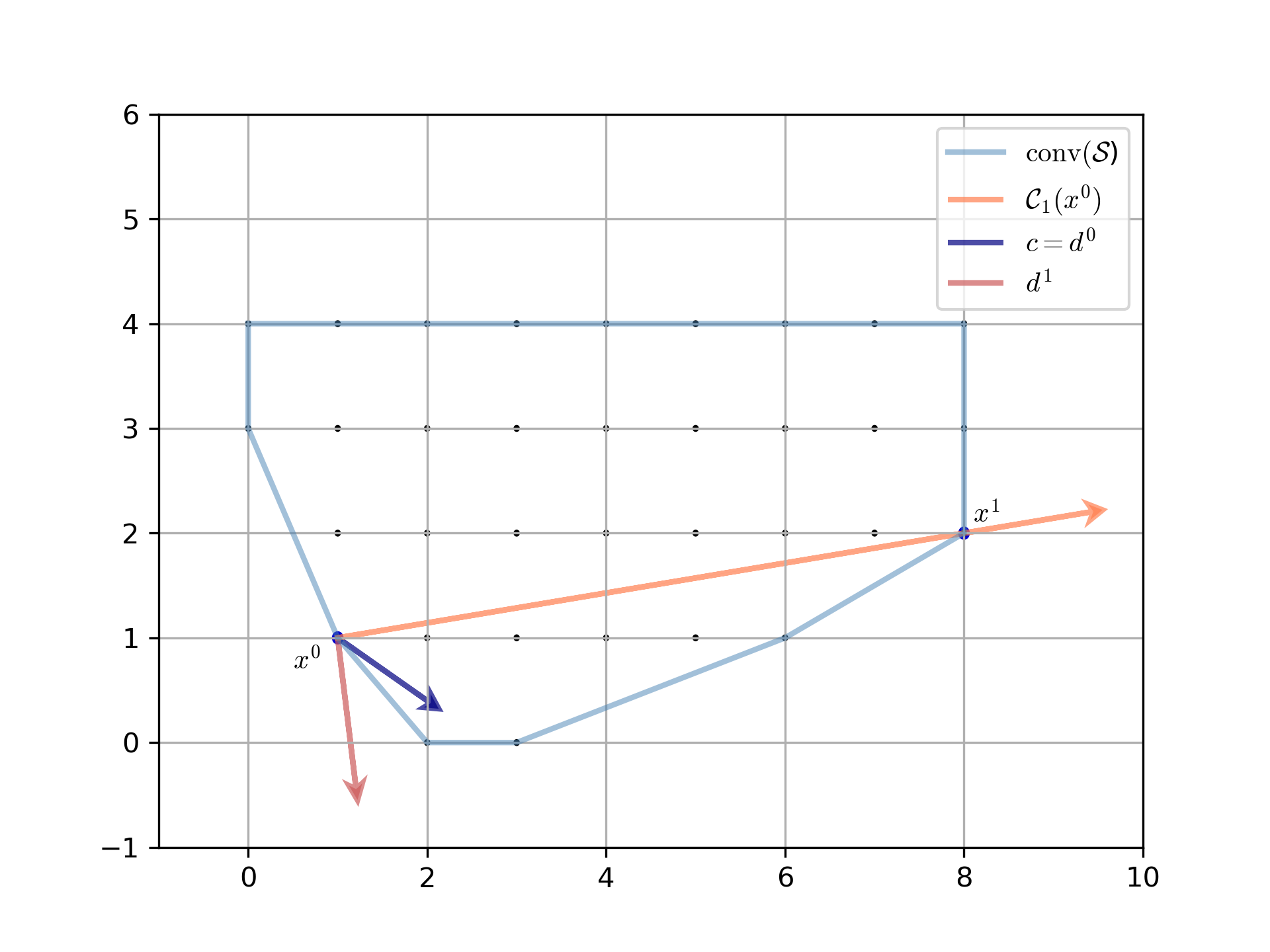
(a) Iteration 1

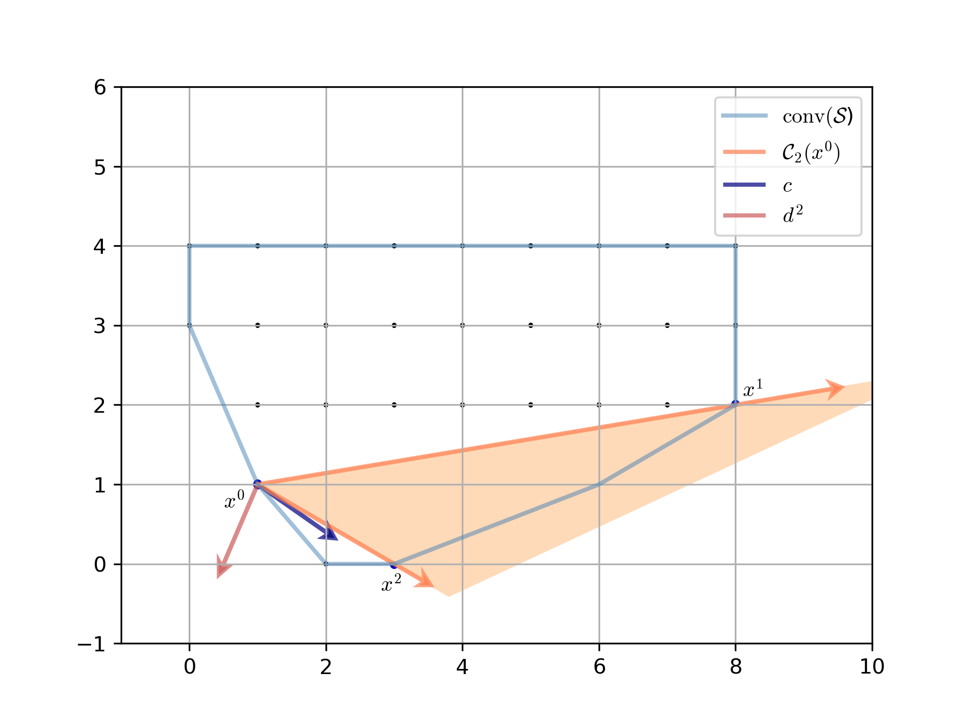
(b) Iteration 2

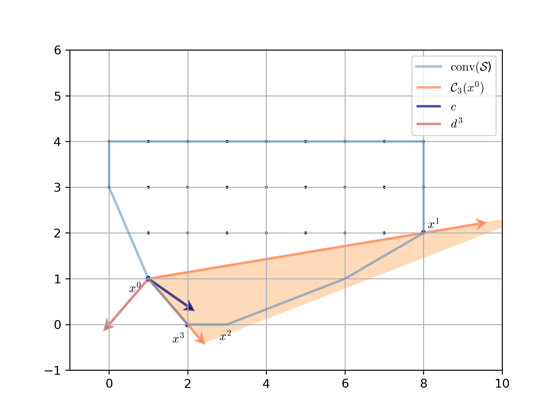
(c) Iteration 3

Figure 4: Pictorial illustration of Algorithm 1

Returning to the relationship of the inverse problem to the separation problem, observe that an essentially unmodified version of Algorithm 1 also solves the generic separation problem for $\operatorname{conv}(\mathcal{S})$ if we interpret $x^{0}$ as the point to be separated rather than the target point. When solving the separation problem, (Inv$\mathcal{P}_{k}$) can be interpreted as the problem of separating $x^{0}$ from $\operatorname{conv}(\mathcal{E}_{k})$. To see this, note that the dual of (Inv$\mathcal{P}_{k}$) is the problem of determining whether $x^{0}$ can be expressed as a convex combination of the members of $\mathcal{E}_{k}$, i.e., the membership problem for $\operatorname{conv}(\mathcal{E}_{k})$. When $x^{0}\not\in\operatorname{conv}(\mathcal{E}_{k})$, the Farkas proof of the infeasibility of this LP is an inequality valid for $\operatorname{conv}(\mathcal{E}_{k})$ and violated by $x^{0}$. ($\mathcal{P}_{k}$) is then interpreted as the problem of determining whether that same inequality is valid for the full feasible set $\operatorname{conv}(\mathcal{S})$, i.e., determining whether there is a member of $\mathcal{S}$ that violates the inequality, exactly as in the inverse case.

Figure 5 illustrates the application of the algorithm for the instance from Figure 4. The only modification is that we replace the objective function of the master problem (Inv$\mathcal{P}_{k}$) with one measuring the degree of violation of $x^{0}$, which is a standard measure of effectiveness for generated valid inequalities. Even without this modification, a violated valid inequality will be generated, but the change is to show that the standard separation problem, in which there is no estimated objective, can also be solved with this algorithm. Inequalities generated in this way are sometimes called Fenchel cuts (Boyd, 1994).

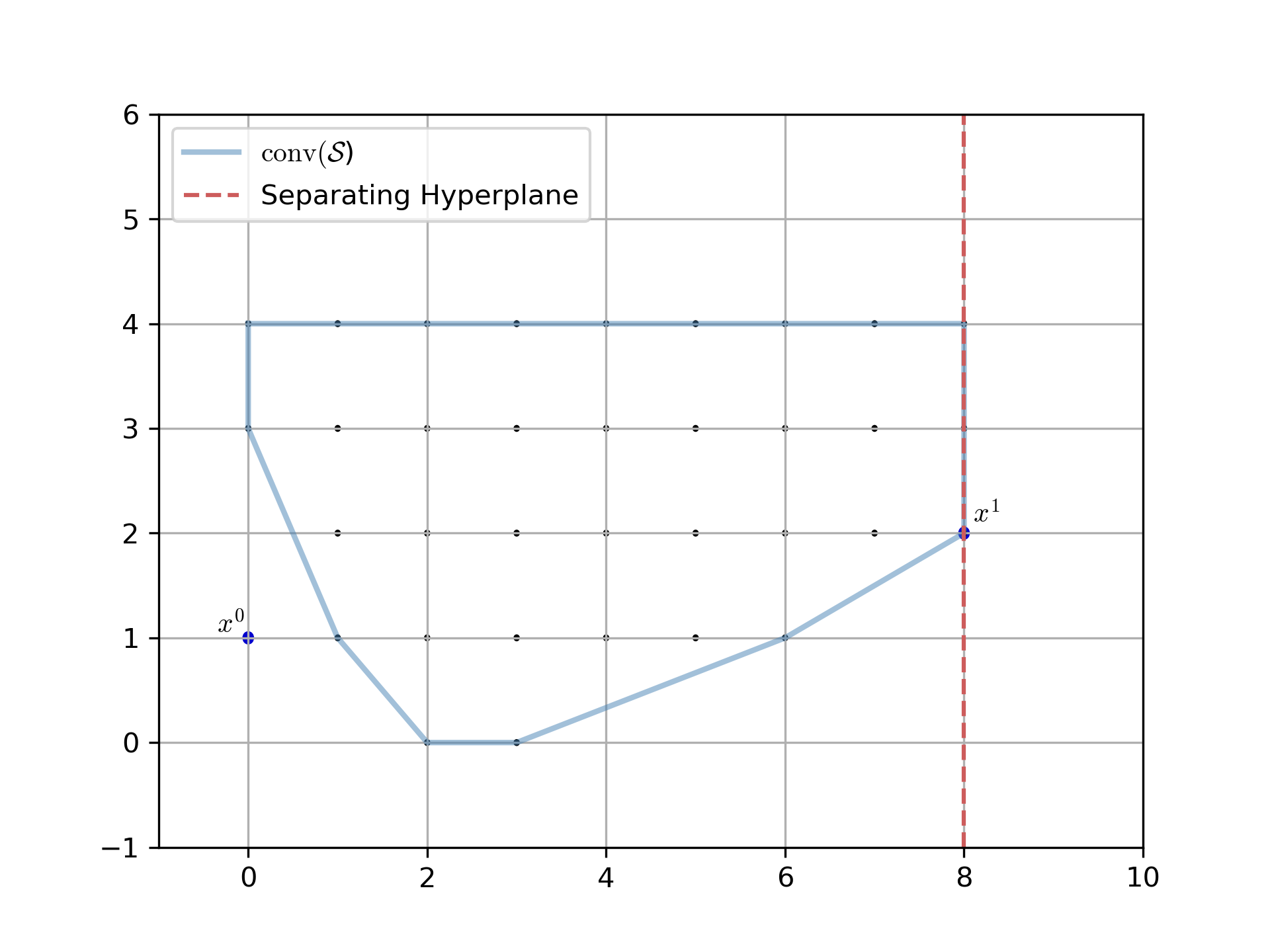
(a) Iteration 1

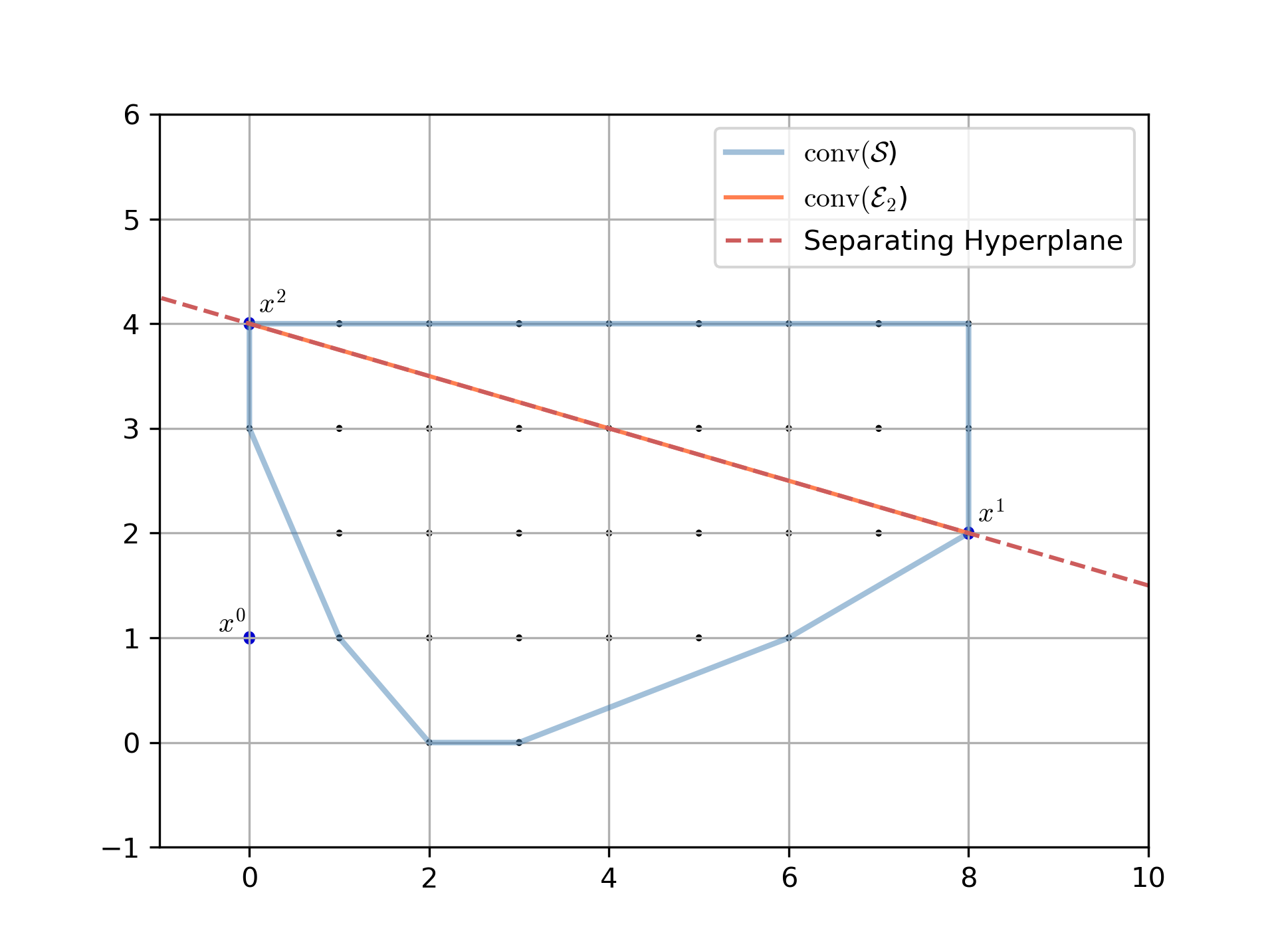
(b) Iteration 2

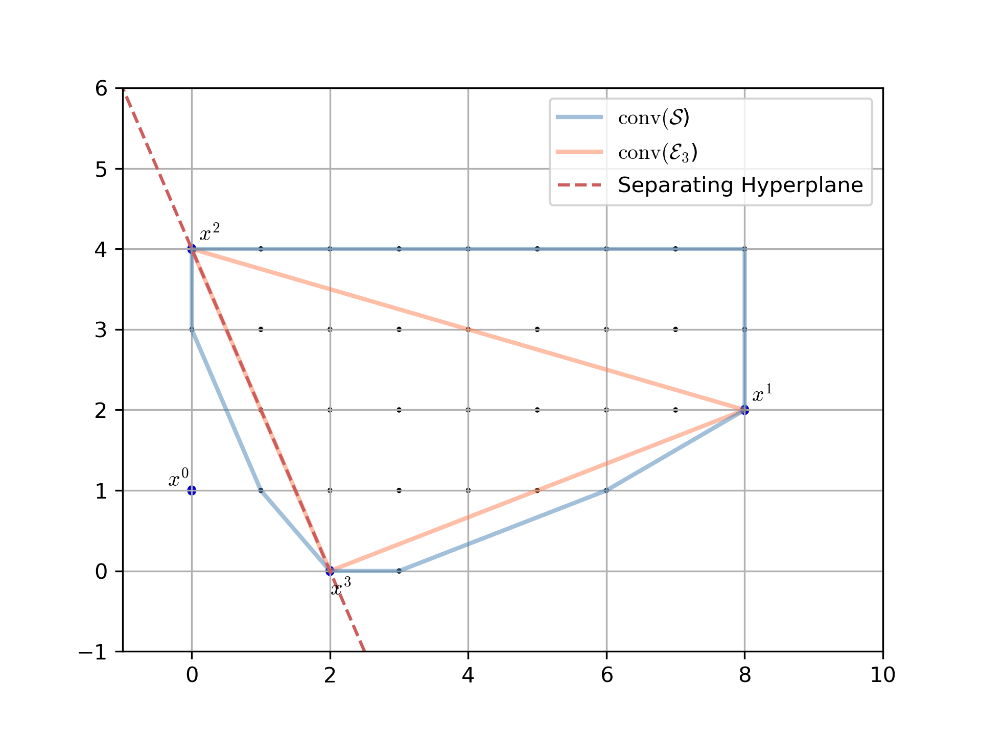
(c) Iteration 3

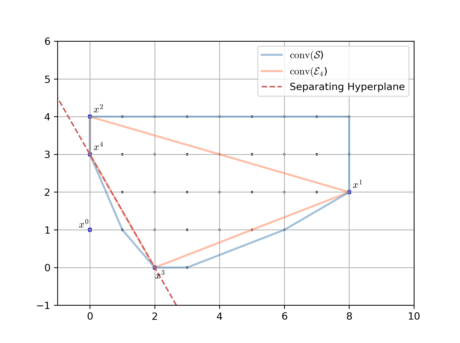
(d) Iteration 4

(e) Iteration 5

Figure 5: Pictorial illustration of algorithm for generating Fenchel cut

3 Computational Complexity

In this section, we briefly review the major concepts in complexity theory and the classes into which (the decision versions of) optimizations problems are generally placed, as well as provide archetypal examples of the kinds of problems that fall into these classes. We mainly follow the framework of Garey and Johnson (1979), but since the material here will be familiar to most readers, we omit many details and refer the reader to either Garey and Johnson (1979) or the sweeping introduction to complexity given by Arora and Barak (2007) for a deeper introduction. We provide this brief, self-contained overview here to emphasize some concepts that are important but lesser known in the mathematical optimization literature. Among these are the definitions of the complexity classes ${\mathsf{D}}^{{\mathsf{P}}}$ and $\Delta_{2}^{p}$, which play a role in our results below, as well as the distinction between the polynomial Turing reductions introduced by Cook (1971) in his seminal work and the polynomial many-to-one reductions introduced by Karp (1972).

The fundamentals of complexity theory and ${\mathsf{NP}}$-completeness as laid out in the papers of Cook (1971),  Karp (1972), Edmonds (1971), and others provide a rigorous framework within which problems arising in discrete optimization can be analyzed. The origins of the theory can be traced back to the earlier work on the Entscheidungsproblem by Turing (1937) and perhaps for that reason, it was originally developed to analyze decision problems, e.g., problems where the output is YES or NO. Although there exists a theory of complexity that applies directly to optimization problems (Krentel, 1987a, 1988; Vollmer and Wagner, 1995)), most analyses are done by converting the optimization problem to an equivalent decision problem form.

The decision problem form typically used for most discrete optimization problems is that of determining whether a given primal bound is valid (upper bound in the case of minimization or lower bound in the case of maximization), though we argue later that verification of the optimal value is more natural. For most problems of current practical interest, verification of the primal bound is either in the class ${\mathsf{P}}$ or the class ${\mathsf{NP}}$. Notable exceptions are the bilevel (and other multilevel) optimization problems, whose decision versions are in higher levels of the so-called polynomial-time hierarchy(Stockmeyer, 1976a).

3.1 Definitions

In the framework of Garey and Johnson (1979), an algorithm is a procedure implemented using the well-known logic of a deterministic Turing machine (DTM), a simple model of a computer capable of sequentially executing a single program (we introduce a “nondeterministic” variant below). The input to the algorithm is a string in a given alphabet, which we assume is simply $\{0,1\}$, since this is the alphabet on all modern computing devices. As such, the set of all possible input strings is denoted $\{0,1\}^{*}$. A problem (or problem class) is defined by describing what set of input strings (called instances) should produce the answer YES. In other words, each subset $L$ of $\{0,1\}^{*}$, formally called a language in complexity theory, defines a different problem for which algorithms can be developed and analyzed. An algorithm is specified by describing its implementation as a DTM and is said to solve such a problem if the DTM correctly outputs YES if and only if the input string is in $L$. In this case, we say the DTM recognizes the language $L$ and that members of $L$ are the instances accepted by the DTM.

Running Time and Complexity.

The running time of an algorithm for a given problem is the worst-case number of steps/operations required by the associated DTM taken over all instances of that problem. This worst case is usually expressed as a function of the “size” of the input, since the worst case would otherwise be unbounded for any class with arbitrarily large instances. The size of the input is formally defined to be its encoding length, which is the length of the string representing the input in the given alphabet. Since we take the alphabet to be $\{0,1\}$, the encoding length of an integer $n$ is

$$\langle n\rangle=1+\lceil\log_{2}(|n|+1)\rceil.$$

Further, the encoding length of a rational number $r=p/q$ is $\langle r\rangle=\langle p\rangle+\langle q\rangle$. Encoding lengths play an important role in the complexity proofs of  Section 4 below. We discuss these concepts in more detail in Section 3.3, but refer the reader to the book of Grötschel et al. (1993) for detailed coverage of definitions and concepts.

The computational complexity of a given problem is the running time (function) of the “best” algorithm, where best is defined by ordering the running time functions according to their asymptotic growth rate (roughly speaking, two functions are compared asymptotically by taking the limit of their ratio as the instance size approaches infinity). For most problems of practical interest, the exact complexity is not known, so another way of comparing problems is by placing them into equivalence classes according to the notion of equivalence yielded by the operation of reduction.

Reduction.

A reduction is the means by which an algorithm for one class of problems (specified by, say, language $L_{1}$) can be used as a subroutine within an algorithm for another class of problems (specified by, say, language $L_{2}$). It is also the means by which problem equivalence and complexity classes are defined.

In what follows, we refer to two notions of reduction, and the difference between them is important. The notion that is most relevant in the theory of NP-completeness is the polynomial many-to-one reduction of Karp (1972), commonly referred to as Karp reduction. There is a Karp reduction from a problem specified by language $L_{2}$ to a problem specified by a language $L_{1}$ if there exists a mapping $f:\{0,1\}^{*}\rightarrow\{0,1\}^{*}$ such that

• $f(x)$ is computable in time polynomial in $\langle x\rangle$ and

• $x\in L_{2}$ if and only if $f(x)\in L_{1}$.

Thus, if we have an algorithm (DTM) for recognizing the language $L_{1}$ and such a mapping $f$, we implicitly have an algorithm for recognizing $L_{2}$. In this case, we say there is a Karp reduction from $L_{2}$ to $L_{1}$.

A second notion of reduction is the polynomial Turing reduction, commonly referred to as Cook reduction, introduced by Cook (1971) in his seminal work. This type of reduction is defined in terms of oracles. An oracle is a conceptual subroutine that can solve a given problem or class of problems in constant time. Roughly speaking, the oracle complexity of a problem is its complexity given the theoretical existence of a certain oracle. There is a Cook reduction from a problem specified by language $L_{2}$ to a problem specified by language $L_{1}$ if there is a polynomial-time algorithm for solving $L_{2}$ that utilizes an oracle for $L_{1}$. Hence, the only requirement is that the number of calls to the oracle must be bounded by a polynomial. The difference between Karp reduction and Cook reduction is that Karp reduction can be thought of as allowing only a single call to the oracle as the last step of the algorithm, whereas Cook reduction allows a polynomial number of calls to the oracle. There are a range of other notions of reduction that utilize other different bounds on the number of oracle calls (Krentel, 1987b).

Decision problems specified by languages $L_{1}$ and $L_{2}$ are said to be equivalent if there is a reduction in both directions—$L_{1}$ reduces to $L_{2}$ and $L_{2}$ reduces to $L_{1}$. Equivalence can be defined using either the Karp or Cook notions of reduction. It is conjectured (though not known; see Beigel and Fortnow (2003)) that these notions of equivalence are distinct and yield different equivalence classes of problems. In fact, assuming that ${\mathsf{NP}}\not={\mathsf{coNP}}$ (which is thought to be highly likely), they must be distinct notions, since a problem specified by any language is trivially seen to be Cook-equivalent to the problem specified by its complement. To Cook-reduce one problem to the other, simply solve the complement and negate the answer. Hence, Cook reduction cannot be used to separate ${\mathsf{NP}}$ from ${\mathsf{coNP}}$. This ability to separate ${\mathsf{NP}}$ from ${\mathsf{coNP}}$ makes Karp reduction a stronger notion and is part of the rationale for its use as the basis for the theory of ${\mathsf{NP}}$-completeness in Garey and Johnson (1979).

A problem in a complexity class is said to be complete for the class if every other problem in the class can be reduced to it. Informally, this means that the complete problems are at least as difficult to solve as any other problem in the class (in a worst-case sense). Completeness of a given problem in a given complexity class can be shown by providing a reduction from a problem already known to be a complete problem for the given class. Equivalence, as described above, is an equivalence relation in the mathematical sense and can thus be used to define equivalence classes for problems. The complete problems for a class are exactly those in the largest such equivalence class that is contained in the class. For the reasons described above, the set of complete problems is different under Karp and Cook, assuming ${\mathsf{NP}}\not={\mathsf{coNP}}$ (see Lutz and Mayordomo (1995)).

Certificates.

Finally, we have the concept of a certificate. A certificate is a string that, when concatenated with the original input string, forms a (longer) input string to an associated decision problem, which we informally call the verification problem, that yields the same output as the original one (but can presumably be solved more efficiently). A certificate can be viewed as a proof of the result of a computation. When produced by an algorithm for solving the original problem, the certificate serves to certify the result of that computation after the fact. The efficiency with which such proofs can be checked is another property of classes of problems (like the running time) that can be used to partition problems into classes according to difficulty. We discuss more about the use of certificates and their formal definition in particular contexts below.

3.2 Complexity Classes

Class ${\mathsf{P}}$.

The most well-known class is ${\mathsf{P}}$, the class of decision problems that can be solved in polynomial time on a DTM (Stockmeyer, 1976a). Alternatively, the class ${\mathsf{P}}$ can be defined as the smallest equivalence class of problems according to the polynomial equivalence relation described earlier. Note that for problems in ${\mathsf{P}}$, there is no distinction between equivalence according to Karp and Cook. The decision versions of linear optimization problems (equivalent to the problem of checking whether a system of inequalities has a solution), the decision versions of minimum cost network flow problems, and other related problems are all in this class. The well-known problem of checking whether a system of linear inequalities has a feasible solution is a prototypical problem in ${\mathsf{P}}$.

Class ${\mathsf{NP}}$.

${\mathsf{NP}}$ is the class of problems that can be solved in polynomial time by a nondeterministic Turing machine (NDTM). Informally, an NDTM is a Turing machine with an infinite number of parallel processors. With such a machine, if there is a branch in the algorithm representing two possible execution paths, we can conceptually follow both branches simultaneously (in parallel), whereas we would need to explore the branches sequentially in a DTM. A search algorithm, for example, may be efficiently implemented on an NDTM by following all possible search paths simultaneously, even if there are exponentially many of them.

The running time of an algorithm on an NDTM is the number of steps it takes for some execution path to reach an accepting state (a state that proves the correct output is YES). As a concrete example, consider the problem of determining whether there exists a binary vector satisfying a system of linear inequalities. A search algorithm that enumerates the exponentially many solutions through a simple depth-first recursion would have exponential running time if implemented using a DTM, while the running time on an NDTM would be the time to construct and check the feasibility of one solution.

This last observation leads to an alternative definition of ${\mathsf{NP}}$ as the class of decision problems for which there exists a certificate for which there is a DTM that solves the verification problem in time polynomial in the length of the input when the output is YES. In fact, these two informal definitions can be formalized and shown to be equivalent.

Intuitively, the idea is that the certificate can be taken to be an encoding of an execution path that leads to a program state that proves the output is YES. Thus, the (deterministic) algorithm for verification is similar to the original nondeterministic algorithm except that it is able to avoid the “dead ends” which are explored in parallel in a nondeterministic algorithm. Formally, if $L\in{\mathsf{NP}}$, then there exists $L^{C}\in{\mathsf{P}}$ such that

$$x\in L\Leftrightarrow\;\; \exists y\in\{0,1\}^{*}\text{ such that }(x,y)\in L^{C}\text{ and}$$

$$\text{$\langle y\rangle$ is bounded by some polynomial function of $\langle x\rangle$}.$$

In this case, $y$ is the certificate. Because such a certificate has an encoding length polynomial in the encoding length of $x$ and can be verified in time polynomial in the encoding length of $x$, such certificates are sometimes said to be short and ${\mathsf{NP}}$ is said to be the class of decision problems having a “short certificate.”

In general, problems in ${\mathsf{NP}}$ concern existential questions, such as whether there exists an element of a set with a given property (alternatively, whether the set of all elements with a given property is nonempty). Even when no algorithm for finding such an element is known, we may still be able to efficiently verify that an element given to us has the desired property. For example, the primal bound verification problem for (MILP) (usually referred to in the literature as the decision version of MILP) is a prototypical problem in this class and is defined as follows.

Definition 2.

MILP Primal Bound Verification Problem (MPVP)

• INPUT: $\alpha\in\mathbb{Q}$, $d\in\mathbb{Q}^{n}$, $A\in\mathbb{Q}^{m\times n}$, $b\in\mathbb{Q}^{m}$, and $r\in\mathbb{N}$, where $(A,b,r)$ is an encoding of the set $\mathcal{S}$ in (MILP) and $(d,\mathcal{S})$ is the input to (MILP).

• OUTPUT: YES, if there exists $x\in\mathcal{S}$ such that $d^{\top}x\geq\alpha$, NO otherwise.

The MPVP is in ${\mathsf{NP}}$ since, when the answer is YES, there always exists $x\in\mathcal{S}$ that is itself such a certificate, i.e., has encoding length polynomially bounded by the encoding length of the problem input and can be verified in polynomial time to be in $\mathcal{S}$ (Papadimitriou, 1981).

The set of problems complete for ${\mathsf{NP}}$ (as defined earlier) is known simply as ${\mathsf{NP}}$-complete. The first problem shown to be complete for class ${\mathsf{NP}}$ was the satisfiability (SAT) problem (Cook, 1971). It was proved to be complete by providing a Karp reduction of any problem that can be solved by an NDTM to the SAT problem. The MPVP is complete for ${\mathsf{NP}}$ because SAT can be Karp-reduced to it. It is well-known that the question of whether ${\mathsf{P}}={\mathsf{NP}}$ is currently unresolved, though it is widely believed that they are distinct classes (Aaronson, 2017).

Class ${\mathsf{coNP}}$.

The class ${\mathsf{coNP}}$ consists of languages whose complement is in ${\mathsf{NP}}$. Just as problems in ${\mathsf{NP}}$ typically concern existential questions, problems in ${\mathsf{coNP}}$ usually concern the question of whether all elements of a set have a given property (alternatively, whether the set of all elements with a given property is empty). As such, these problems are not expected to have certificates (for the YES answer) that can be efficiently verified in the sense defined earlier. Rather, problems in this class are those for which there exists a string that can be used to certify the output (in time polynomial in the encoding length of the input) when the answer is NO. For example, we may produce an element of the set that doesn’t have the desired property. The MILP Dual Bound Verification Problem is an example of a prototypical problem in ${\mathsf{coNP}}$.

Definition 3.

MILP Dual Bound Verification Problem (MDVP)

• INPUT: $\alpha\in\mathbb{Q}$, $d\in\mathbb{Q}^{n}$, $A\in\mathbb{Q}^{m\times n}$, $b\in\mathbb{Q}^{m}$, and $r\in\mathbb{N}$, where $(A,b,r)$ is an encoding of the set $\mathcal{S}$ in (MILP) and $(d,\mathcal{S})$ is the input to (MILP).

• OUTPUT: YES, if $d^{\top}x\leq\alpha$ for all $x\in\mathcal{S}$, NO otherwise.

The input to the MDVP is ($\alpha$, $d$, $A$, $b$, $r$), as in the case of the MPVP. The MDVP is in ${\mathsf{coNP}}$ because when the output is NO, there must be a member of $\mathcal{S}$ with an objective value strictly greater than $\alpha$, which serves as the certificate.

Class ${\mathsf{D}}^{{\mathsf{P}}}$.

While ${\mathsf{NP}}$ and ${\mathsf{coNP}}$ are both well-known classes, the class ${\mathsf{D}}^{{\mathsf{P}}}$ introduced by Papadimitriou and Yannakakis (1982) is not as well-known. It is the class of problems associated with languages that are intersections of a language from ${\mathsf{NP}}$ and a language from ${\mathsf{coNP}}$. A prototypical problem complete for ${\mathsf{D}}^{{\mathsf{P}}}$ is the MILP Optimal Value Verification Problem (MOVP), defined as follows.

Definition 4.

MILP Optimal Value Verification Problem (MOVP)

• INPUT: $\alpha\in\mathbb{Q}$, $d\in\mathbb{Q}^{n}$, $A\in\mathbb{Q}^{m\times n}$, $b\in\mathbb{Q}^{m}$, and $r\in\mathbb{N}$, where $(A,b,r)$ is an encoding of the set $\mathcal{S}$ in (MILP) and $(d,\mathcal{S})$ is the input to (MILP).

• OUTPUT: YES, if $\max_{x\in\mathcal{S}}d^{\top}x:=\alpha$, NO otherwise.

It is easy to see that the language associated with MOVP is the intersection of the languages of the MPVP and the MDVP, since the output of MOVP is YES if and only if the outputs of both the MPVP and the MDVP are YES, i.e., $\alpha$ is both a primal and a dual bound for (MILP).

In view of our later results, one outcome of this work is the suggestion that the MOVP is a more natural decision problem to associate with discrete optimization problems than the more traditional MPVP and should be more widely adopted in proving complexity results. Most algorithms for discrete optimization are based on iterative construction of separate certificates for the validity of the primal and dual bound, which must be equal to certify optimality. Given certificates for the primal and dual bound verification problems, a certificate for the optimal value verification problem can thus be constructed directly. The class ${\mathsf{D}}^{{\mathsf{P}}}$ thus contains the optimal value verification problem associated with (MILP), whereas it is the associated MPVP that is contained in the class ${\mathsf{NP}}$-complete. We find this is somewhat unsatisfying, since the original problem (MILP) is only Cook-reducible to the MPVP.

The Polynomial Hierarchy.

Further classes in the so-called polynomial-time hierarchy (${\mathsf{PH}}$), described in the seminal work of Stockmeyer (1976a), can be defined recursively using oracle computation. The notation ${\mathsf{A}}^{{\mathsf{B}}}$ is used to denote the class of problems that are in ${\mathsf{A}}$, assuming the existence of an oracle for problems in class ${\mathsf{B}}$.

Using this concept, $\Delta_{2}^{p}$ is the class of decision problems that can be solved in polynomial time given an ${\mathsf{NP}}$ oracle, i.e., the class ${\mathsf{P}}^{\mathsf{NP}}$. This class is a member of the second level of ${\mathsf{PH}}$. Further levels are defined according to the following recursion.

$$\Delta^{p}_{0} :=\Sigma^{p}_{0}:=\Pi^{p}_{0}:={\mathsf{P}},$$

$$\Delta^{p}_{k+1} :={\mathsf{P}}^{\Sigma^{p}_{k}},$$

$$\Sigma^{p}_{k+1} :={\mathsf{NP}}^{\Sigma^{p}_{k}},\text{ and}$$

$$\Pi^{p}_{k+1} :={\mathsf{coNP}}^{\Sigma^{p}_{k}}.$$

${\mathsf{PH}}$ is the union of all levels of the hierarchy. There is also an equivalent definition that uses the notion of certificates. Roughly speaking, each level of the hierarchy consists of problems with certificates of polynomial size, but whose verification problem is in the class one level lower in the hierarchy. In other words, the problem of verifying a certificate for a problem in $\Sigma_{i}^{p}$ is a problem in the class $\Sigma_{i-1}^{p}$ (Stockmeyer, 1976b).

Figure 6 illustrates class $\Delta_{2}^{p}$ relative to ${\mathsf{D}}^{{\mathsf{P}}}$, ${\mathsf{NP}}$, ${\mathsf{coNP}}$, and ${\mathsf{P}}$, assuming ${\mathsf{P}}\neq{\mathsf{NP}}$. If ${\mathsf{P}}={\mathsf{NP}}$, we conclude that all classes are equivalent, i.e., $\Delta_{2}^{p}={\mathsf{D}}^{{\mathsf{P}}}={\mathsf{NP}}={\mathsf{coNP}}={\mathsf{P}}$. This theoretical possibility is known as the collapse of ${\mathsf{PH}}$ to its first level (Papadimitriou, 2003) and is thought to be highly unlikely. A prototypical problem complete for $\Delta_{2}^{p}$ is the problem of deciding whether a given MILP has a unique solution(Papadimitriou, 2003).

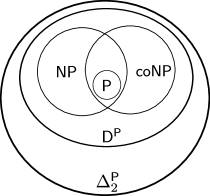
Figure 6: Complexity classes $\Delta_{2}^{p}$, ${\mathsf{D}}^{{\mathsf{P}}}$, ${\mathsf{NP}}$, ${\mathsf{coNP}}$, and ${\mathsf{P}}$, assuming ${\mathsf{P}}\neq{\mathsf{NP}}$

3.3 Optimization and Separation

The concepts of reduction and polynomial equivalence can be extended to problems other than decision problems, but this requires some additional care and machinery. Decision problems can be (and often are) reduced to optimization problems, in a fashion similar to that described earlier, in an attempt to classify them. When a problem that is complete for a given class in the polynomial hierarchy can be Karp-reduced to an optimization problem, we refer to the optimization problem as hard for the class. When a decision problem that is complete for ${\mathsf{NP}}$ can be Karp-reduced to an optimization problem, for example, the optimization problem is classified as ${\mathsf{NP}}$-hard. This does not, however, require that the decision version of this optimization problem is a member of the class itself. In reality, it may be on some higher level of the polynomial hierarchy. Hardness results can therefore be somewhat misleading in some cases.

In their foundational work, Grötschel et al. (1993) develop a detailed theoretical basis for the claim that the separation problem for an implicitly defined polyhedron is polynomially equivalent to the optimization problem over that same polyhedron. This is done very carefully, beginning from certain decision problems and proceeding to show their equivalence to related optimization problems. The notion of reduction used, however, is Cook reduction, which means that the results do not directly tell us whether there are decision versions of the problems discussed that are complete for the same class within ${\mathsf{PH}}$. The results discussed below, in contrast, use Karp reduction to show that there are decision versions of the inverse and forward optimization problems that are complete for the same complexity class within ${\mathsf{PH}}$.

Using an optimization oracle to solve the separation problem (and vice versa) involves converting between different representations of a given polyhedron. In particular, we consider (implicit) descriptions in terms of the half-spaces associated with facet-defining valid inequalities, so-called H-representations, and in terms of generators (vertices and extreme rays), so-called V-representations. There is a formal mathematical duality relating these two forms of polyhedral representation, which underlies the notion of polarity mentioned earlier and is at the heart of the equivalence between optimization and separation. It is this very same duality that is also at the heart of the equivalence between optimization problems and their inverse versions. This can be most clearly seen by the fact that the feasible region $\mathcal{C}^{\circ}(x^{0})$ of the inverse problem is the polar of $\mathcal{C}(x^{0})$, a conic set that contains $\operatorname{conv}(\mathcal{S})$, as we have already described.

The framework laid out by Grötschel et al. (1993) emphasizes that the efficiency with which the various representations can be manipulated algorithmically depends inherently and crucially on, among other things, the encoding length of the elements of these representations. For the purposes of their analysis, Grötschel et al. (1993) defined the notions of the vertex complexity and facet complexity of a polyhedron, which we repeat here, due to their relevance in the remainder of the paper.

Definition 5.

(Grötschel et al. (1993))

1. A polyhedron $\mathcal{P}\subseteq\mathbb{R}^{n}$ has facet complexity of at most $\varphi$ if there exists a rational system of inequalities (known as an H-representation) describing the polyhedron in which the encoding length of each inequality is at most $\varphi$.

2. Similarly, the vertex complexity of $\mathcal{P}$ is at most $\nu$ if there exist finite sets $V,E$ such that $\mathcal{P}=\operatorname{conv}(V)+\operatorname{cone}(E)$ (known as a V-representation) and such that each of the vectors in $V$ and $E$ has encoding length at most $\nu$.

It is important to point out that these definitions are not given in terms of the encoding length of a full description of $\mathcal{P}$ because $\mathcal{P}$ may be an implicitly defined polyhedron whose description is never fully constructed. What is explicitly constructed are the components of the description (extreme points and facet-defining inequalities). The importance of the facet complexity and vertex complexity in the analysis is primarily that they provide bounds on the norms of these vectors. The ability to derive such bounds is a crucial element in the overall framework they present. The following are relevant results from Grötschel et al. (1993).

Proposition 1.

(Grötschel et al. (1993))

1. (1.3.3) For any $r\in\mathbb{Q}$, $2^{-\langle r\rangle+2}\leq|r|\leq 2^{\langle r\rangle-1}-1$.

2. (1.3.3) For any $x\in\mathbb{Q}^{n}$, $\|x\|_{p}<2^{\langle x\rangle-n}$ for $p\geq 1$.

3. (6.2.9) If $\mathcal{P}$ is a polyhedron with vertex complexity at most $\nu$ and $(a,b)\in\mathbb{Z}^{n+1}$ is such that

   $$a^{\top}x\leq b+2^{-\nu-1}$$

   holds for all $x\in\mathcal{P}$, then $(a,b)$ is valid for $\mathcal{P}$.

In other words, the facet complexity and the encoding lengths of the vectors involved specify a “granularity” that can allow us to, for example, replace a “$<$” with a “$\leq$” if we can bound the encoding length of the numbers involved.

Utilizing the above definitions, the result showing the equivalence of optimization and separation can be formally stated as follows.

Theorem 1.

(Grötschel et al. (1993)) Let $\mathcal{P}\subseteq\mathbb{R}^{n}$ be a polyhedron with facet complexity $\varphi$. Given an oracle for any one of

• the dual bound verification problem over $\mathcal{P}$ with linear objective coefficient $d\in\mathbb{Q}^{n}$,

• the separation problem for $\mathcal{P}$ with respect to $\hat{x}\in\mathbb{Q}^{n}$, or

• the primal bound verification problem for $\mathcal{P}$ with linear objective coefficient $d\in\mathbb{Q}^{n}$,

there exists an oracle polynomial-time algorithm for solving either of the other two problems. Further, all three problems are solvable in time polynomial in $n$, $\varphi$, and either $\langle d\rangle$ (in the case of primal or dual bound verification) or $\langle\hat{x}\rangle$ (in the case of separation).

The problem of verifying a given dual bound was called the violation problem by Grötschel et al. (1993). The above result refers only to the facet complexity $\varphi$, but we could also replace it with the vertex complexity $\nu$, since it is easy to show that $\nu\leq 4n^{2}\varphi$. In the remainder of the paper, we refer to the “polyhedral complexity” whenever the facet complexity and vertex complexity can be used interchangeably.

4 Complexity of Inverse MILP 

In this section, we apply the framework discussed in Section 3 to analyze the complexity of the inverse MILP. We follow the traditional approach and describe the complexity of the decision versions. In addition to the standard primal bound verification problem, we also consider the dual bound and optimal value verification problems. We show that the primal bound, dual bound, and optimal value verification problems for the inverse MILP are in the complexity classes ${\mathsf{coNP}}$-complete, ${\mathsf{NP}}$-complete, and ${\mathsf{D}}^{{\mathsf{P}}}$-complete, respectively. Hence, the classes associated with primal and dual bounding problems are reversed when going from MILP to inverse MILP, while the optimal value verification problems are both contained in the same class.

4.1 Polynomially Solvable Cases

The result of Ahuja and Orlin (2001) can be applied directly to observe that there are cases of the inverse MILP that are polynomially solvable. In particular, they showed that the inverse problem can be solved in polynomial time whenever the forward problem is polynomially solvable.

Theorem 2.

(Ahuja and Orlin (2001)) If an optimization problem is polynomially solvable for each linear cost function, then the corresponding inverse problems under the $\ell_{1}$ and $\ell_{\infty}$ norms are polynomially solvable.

Ahuja and Orlin (2001) use Theorem 1 from Grötschel et al. (1993) to conclude that inverse LP, in particular, is polynomially solvable. The separation problem in this case is an LP of polynomial input size and is hence polynomially solvable. The theorem of  Grötschel et al. (1993) shows that both problems are in the class ${\mathsf{P}}$, since Karp and Cook reductions are equivalent for problems in ${\mathsf{P}}$. Theorem 2 also indicates that if a given MILP is polynomially solvable, then the associated inverse problem is also polynomially solvable.

4.2 General Case

In the general case, the MILP constituting the forward problem is not known to be polynomially solvable and so we now consider MILPs whose decision versions are complete for ${\mathsf{NP}}$. Applying the results of Grötschel et al. (1993) straightforwardly, as  Ahuja and Orlin (2001) did, we can easily show that ( ‣ 2) and ( ‣ 2) can be solved in polynomial time, given an oracle for the MPVP, as stated in the following theorem.

Theorem 3.

Given an oracle for the MPVP, ( ‣ 2) and ( ‣ 2) are solvable in time polynomial in $n$, the vertex complexity of $\operatorname{conv}(\mathcal{S}^{+})$, and $\langle c\rangle$.

The above result directly implies that IMILP under $\ell_{1}$ and $\ell_{\infty}$ norms is in fact in the complexity $\Delta_{2}^{{\mathsf{P}}}$, but stronger results are possible, as we show. In the remainder of this section, we assume the norm used is a $p$-norm, as this is needed for some results (in particular, Proposition 1 is crucially used).

Definitions.

We next define decision versions of the inverse MILP analogous to those we defined in the case of MILP. These similarly attempt to verify that a given bound on the objective value is a primal bound, a dual bound, or an exact optimal value. The primal bound verification problem for inverse MILP is as follows.

Definition 6.

Inverse MILP Primal Bound Verification Problem (IMPVP):

• INPUT: $\gamma\in\mathbb{Q}$, $x^{0}\in\mathbb{Q}^{n}$, $A\in\mathbb{Q}^{m\times n}$, $c\in\mathbb{Q}^{n}$, $b\in\mathbb{Q}^{m}$, and $r\in\mathbb{N}$, where $(A,b,r)$ is an encoding of the set $\mathcal{S}$ in (MILP) and $(c,\mathcal{S},x^{0})$ are input data for problem (IMILP).

• OUTPUT: YES, if $\exists d\in\mathcal{C}^{\circ}(x^{0})$ such that $\|c-d\|\leq\gamma$, i.e., $\mathcal{K}(\gamma)\cap\mathcal{C}^{\circ}(x^{0})\not=\emptyset$, NO otherwise.

Similarly, we have the dual bound verification problem for inverse MILP.

Definition 7.

Inverse MILP Dual Bound Verification Problem (IMDVP):

• INPUT: $\gamma\in\mathbb{Q}$, $x^{0}\in\mathbb{Q}^{n}$, $A\in\mathbb{Q}^{m\times n}$, $c\in\mathbb{Q}^{n}$, $b\in\mathbb{Q}^{m}$, and $r\in\mathbb{N}$, where $(A,b,r)$ is an encoding of the set $\mathcal{S}$ in (MILP) and $(c,\mathcal{S},x^{0})$ are input data for problem (IMILP).

• OUTPUT: YES, if $\|c-d\|\geq\gamma$ for all $d\in\mathcal{C}^{\circ}(x^{0})$. Equivalently, $\operatorname{int}\left(\mathcal{K}(\gamma)\right)\cap\mathcal{C}^{\circ}(x^{0})=\emptyset$, NO otherwise.

Finally, we have the optimal value verification problem.

Definition 8.

Inverse MILP Optimal Value Verification Problem (IMOVP):

• INPUT: $\gamma\in\mathbb{Q}$, $x^{0}\in\mathbb{Q}^{n}$, $A\in\mathbb{Q}^{m\times n}$, $c\in\mathbb{Q}^{n}$, $b\in\mathbb{Q}^{m}$, and $r\in\mathbb{N}$, where $(A,b,r)$ is an encoding of the set $\mathcal{S}$ in (MILP) and $(c,\mathcal{S},x^{0})$ are input data for problem (IMILP).

• OUTPUT: YES, if $\min_{d\in\mathcal{K}(y)\cap\mathcal{C}^{\circ}(x^{0})}y=\gamma$, NO otherwise.

In the rest of the section, we formally establish the complexity class membership of each of the above problems and in so doing, illustrate the relationships of the above problem to each other and to their MILP counterparts. We assume from here on that $\operatorname{conv}(\mathcal{S}^{+})$ full-dimensional (and that hence, $\mathcal{C}^{\circ}(x^{0})$ is also full-dimensional) to simplify the exposition.

Informal Discussion.

Before presenting the formal proofs, which are somewhat technical, we informally describe the relationship of the inverse optimization problem to the MILP analogues of the above decision problems, which are described in Section 3.2. Suppose we are given a value $\alpha$ and we wish to determine whether it is a primal bound, a dual bound, or the exact optimal value of (MILP) with objective function vector $c\in\mathbb{Q}^{n}$. Roughly speaking, we can utilize an algorithm for solving (IMILP) to make the determination, as follows. We first construct the target vector

$$x^{\alpha}:=\alpha\frac{c}{\|c\|_{2}^{2}},$$

which has an objective function value (in the forward problem) of $c^{\top}x^{\alpha}=\alpha$ by construction. Now suppose we solve (IMILP) with $x^{\alpha}$ as the target vector and $c$ as the estimated objective function coefficient. Note that $x^{\alpha}$ is not necessarily in $\mathcal{S}$. Solving this inverse problem will yield one of two results.

1. The optimal value of the inverse problem is $0$. This means that $x^{\alpha}\in\operatorname{argmax}_{x\in\mathcal{S}^{+}}c^{\top}x$, which immediately implies that $\alpha\geq\max_{x\in\mathcal{S}}c^{\top}x$ and we have that $\alpha$ is a valid dual bound for (MILP).

2. The optimal value of the inverse problem is strictly positive. Then there must be a point $x\in\mathcal{S}$ for which $c^{\top}x>c^{\top}x^{\alpha}=\alpha$, which means that $\alpha<\max_{x\in\mathcal{S}}c^{\top}x$ and $\alpha$ is a (strict) primal bound for (MILP).

There are a number of challenges to be overcome in moving from this informal argument to the formal reductions in the completeness proofs. One obstacle is that the above argument does not precisely establish the status of $\alpha$ as a bound because we cannot distinguish between when $\alpha$ is a strict dual bound (and hence not a primal bound) and when $\alpha$ is the exact optimal value. This can be overcome essentially by appealing to Proposition 1 to reformulate certain strict inequalities as standard inequalities (see Lemma 3). A second challenge is that we have only described a reduction of a decision version of MILP to an optimization version of the inverse problem and have failed to describe any sort of certificate. The formal proofs provide reductions to decision versions of the inverse problem along with the required short certificates. Despite the additional required machinery, however, the principle at the core of these proofs is the simple one we have just described.

Formal Proofs.

We now present the main results of the paper and their formal proofs. Two lemmas that characterize precisely when a given value $\gamma$ is either a dual bound or a strict dual bound, respectively, for (IMILP) are presented first. These lemmas are the key element underlying the proofs that follow so we first explain the intuition. Recall the instances of (IMILP) illustrated earlier in Figure 2. The output to the IMPVP for these four instances would be NO, NO, YES, and NO, respectively. Note that for the YES instance in Figure 2c, $K(\gamma)\cap\mathcal{C}^{\circ}(x^{0})$ is nonempty, as one would expect, while for the NO instance, this intersection is empty. It would appear that we are thus facing an existential question, so that the YES output would be the easier of the two to verify by simply producing an element of $K(\gamma)\cap\mathcal{C}^{\circ}(x^{0})$.

As it turns out, the above reasoning, though intuitive, is incorrect. The key observation we exploit is that whenever $K(\gamma)\cap\mathcal{C}^{\circ}(x^{0})$ is empty, $\operatorname{conv}(\mathcal{S})\cap\operatorname{int}\left(\mathcal{K}^{*}(\gamma)\right)$ is nonempty and vice versa. Furthermore, there is a short certificate for membership in $\operatorname{conv}(\mathcal{S})\cap\operatorname{int}\left(\mathcal{K}^{*}(\gamma)\right)$. The characterization in terms of $K(\gamma)\cap\mathcal{C}^{\circ}(x^{0})$ can be seen as being in the dual space, whereas the characterization in terms of $\operatorname{conv}(\mathcal{S})\cap\operatorname{int}\left(\mathcal{K}^{*}(\gamma)\right)$ is in the primal space. It is highly unlikely that a short certificate for membership in $\mathcal{C}^{\circ}(x^{0})$ exists and the reason can be understood upon closer examination. It is that we lack an explicit description of $\mathcal{C}^{\circ}(x^{0})$ in terms of generators (a V-representation). We only have access to a partial description of it in terms of valid inequalities (a partial H-representation). Whereas any convex combination of a subset of generators of a polyhedral set must be in the set, a point satisfying a subset of the valid inequalities may not be in the set. Therefore, a partial H-representation is not sufficient for constructing a certificate. Even if we were able to obtain a set of generators algorithmically, we have no short certificate of the fact that they are in fact generators. On the other hand, it is easy to check membership for the points in $\mathcal{S}$ that generate $\operatorname{conv}(\mathcal{S})$. This is fundamentally why verifying a primal bound for (MILP) is in ${\mathsf{NP}}$, whereas verifying a primal bound for (IMILP) is in ${\mathsf{coNP}}$.

The equivalence of the two characterizations described above is formalized below and this is what eventually allows us to prove the existence of a short certificate for $\gamma$ being a dual bound or strict dual bound for (IMILP), respectively.

Lemma 1.

For $\gamma\in\mathbb{Q}$ such that $0\leq\gamma<\|c\|$, we have

$$\mathcal{K}(\gamma)\cap\mathcal{C}^{\circ}(x^{0})=\emptyset \Leftrightarrow\operatorname{conv}(\mathcal{S}^{+})\cap\operatorname{int}\left(\mathcal{K}^{*}(\gamma)\right)\not=\emptyset$$

$$\Leftrightarrow\|c-d\|>\gamma\;\forall d\in\mathcal{C}^{\circ}(x^{0})$$

$$\Leftrightarrow\gamma\textrm{ is a strict dual bound for~{}\eqref{eq:imilp}}$$

$$\Leftrightarrow\gamma\textrm{ is \emph{not} a primal bound for~{}\eqref{eq:imilp}}.$$

Proof.

We prove that $\mathcal{K}(\gamma)\cap\mathcal{C}^{\circ}(x^{0})=\emptyset$ if and only if $\operatorname{conv}(\mathcal{S}^{+})\cap\operatorname{int}\left(\mathcal{K}^{*}(\gamma)\right)\not=\emptyset$. The remaining implications follow by definition.

• For the sake of contradiction, let us assume that both $\mathcal{K}(\gamma)\cap\mathcal{C}^{\circ}(x^{0})=\emptyset$ and $\operatorname{conv}(\mathcal{S}^{+})\cap\operatorname{int}\left(\mathcal{K}^{*}(\gamma)\right)=\emptyset$. Under the assumptions that $\operatorname{conv}(\mathcal{S}^{+})$ is full-dimensional and $0\leq\gamma<\|c\|$, $\operatorname{conv}(\mathcal{S}^{+})$ and $\operatorname{int}\left(\mathcal{K}^{*}(\gamma)\right)$ are both nonempty convex sets, so there exists a hyperplane separating them. In particular, there exists $a\in\mathbb{R}^{n}$ such that

  $$\max_{x\in\operatorname{conv}(\mathcal{S}^{+})}a^{\top}x\leq\min_{x\in\mathcal{K}^{*}(\gamma)}a^{\top}x=\inf_{x\in\operatorname{int}\left(\mathcal{K}^{*}(\gamma)\right)}a^{\top}x.$$ (SEPi)

  The problem on the right-hand side is unbounded when $a\not\in\mathcal{K}(\gamma)$, since then there must exist $x\in\operatorname{int}\left(\mathcal{K}^{*}(\gamma)\right)$ with $a^{\top}x<a^{\top}x^{0}$, which means that $x-x^{0}$ is a ray with negative objective value (recall $\mathcal{K}^{*}(\gamma)$ is a cone). Therefore, we must have $a\in\mathcal{K}(\gamma)$ and it follows that $x^{0}$ is an optimal solution for the problem on the right-hand side. Therefore, we have

  $$\max_{x\in\operatorname{conv}(\mathcal{S}^{+})}a^{\top}x\leq a^{\top}x^{0}.$$

  Since $a\in\mathcal{K}(\gamma)$, then by assumption, $a\not\in\mathcal{C}^{\circ}(x^{0})$, so there exists an $\hat{x}\in\mathcal{S}^{+}$ such that $a^{\top}(x^{0}-\hat{x})<0$. So finally, we have

  $$a^{\top}x^{0}<a^{\top}\hat{x}\leq\max_{x\in\operatorname{conv}(\mathcal{S}^{+})}a^{\top}x\leq a^{\top}x^{0},$$

  which is a contradiction. This completes the proof of the forward direction.

• For the reverse direction, we assume there exists $\overline{x}\in\operatorname{conv}(\mathcal{S}^{+})\cap\operatorname{int}\left(\mathcal{K}^{*}(\gamma)\right)$. Since $\overline{x}\in\operatorname{conv}(\mathcal{S}^{+})$, there exists $\{x^{1},x^{2},\dots,x^{k}\}\subseteq\mathcal{S}^{+}$ and $\lambda\in\mathbb{Q}^{k}_{+}$ such that $\overline{x}=\sum_{i=1}^{k}\lambda_{i}x^{i}$, $\sum_{i=1}^{k}\lambda_{i}=1$, and $k\leq n+1$. Now, let an arbitrary $d\in\mathcal{K}(\gamma)$ be given. Since $\gamma<\|c\|$, we have $d\not=0$. Then, since $\overline{x}\in\operatorname{int}\left(\mathcal{K}^{*}(\gamma)\right)$, we have that

  $$d^{\top}\left(x^{0}-\overline{x}\right)<0 \Leftrightarrow d^{\top}x^{0}-\left(\sum_{i=1}^{k}\lambda_{i}x^{i}\right)<0$$

  $$\Leftrightarrow d^{\top}\left(\sum_{i=1}^{k}\lambda_{i}x^{0}-\sum_{i=1}^{k}\lambda_{i}x^{i}\right)<0$$

  $$\Leftrightarrow\sum_{i=1}^{k}\lambda_{i}d^{\top}\left(x^{0}-x^{i}\right)<0$$

  $$\Rightarrow\exists j\in\{1,\dots,k\}\textrm{ such that }d^{\top}(x^{0}-x^{j})<0$$

  $$\Rightarrow d\notin\mathcal{C}^{\circ}(x^{0}).$$

  Since $d$ was chosen arbitrarily, we have that $\mathcal{K}(\gamma)\cap\mathcal{C}^{\circ}(x^{0})=\emptyset$. This completes the proof of the reverse direction.

∎

When $\gamma=0$, we have that $\mathcal{K}^{*}(\gamma)$ is the half-space $\{x\in\mathbb{R}^{n}\mid c^{\top}x\geq c^{\top}x^{0}\}$, which further hints at the relationship between the inverse dual bounding problem and both the MILP primal bounding problem and the separation problem. A slightly modified version of Lemma 1 characterizes when $\gamma$ is a dual bound, but not necessarily strict. Note that unlike the characterization in Lemma 1, this characterization doesn’t hold when $\gamma=0$, which is perhaps not surprising, since the specific form of objective function we have chosen ensures that zero is always a valid lower bound. As such, this information cannot be helpful in distinguishing outcomes for the purpose of the reductions described shortly.

Lemma 2.

For $\gamma\in\mathbb{Q}$ such that $0<\gamma<\|c\|$, we have

$$\operatorname{int}\left(K(\gamma)\right)\cap\mathcal{C}^{\circ}(x^{0})=\emptyset \Leftrightarrow\operatorname{conv}(\mathcal{S}^{+})\cap\left(\mathcal{K}^{*}(\gamma)\setminus\{x^{0}\}\right)\not=\emptyset$$

$$\Leftrightarrow\|c-d\|\geq\gamma\;\forall d\in\mathcal{C}^{\circ}(x^{0})$$

$$\Leftrightarrow\gamma\textrm{ is a dual bound for~{}\eqref{eq:imilp}}$$

$$\Leftrightarrow\gamma\textrm{ is \emph{not} a strict primal bound for~{}\eqref{eq:imilp}}$$

We now present the main theorems.

Theorem 4.

The IMPVP is in ${\mathsf{coNP}}$.

Proof.

We prove the theorem by showing the existence of a short certificate when the output to the problem is NO. Therefore, let an instance $(\gamma,x^{0},c,A,b,r)$ of the IMPVP for which the output is NO be given along with relevant input data. Since the output is NO, we must have that $\gamma<\|c\|$, since $d=0$ is a valid solution otherwise. By the characterization of Lemma 1, the NO answer is equivalent to the condition $\mathcal{K}(\gamma)\cap\mathcal{C}^{\circ}(x^{0})=\emptyset$, as well as to the existence of $\overline{x}\in\operatorname{conv}(\mathcal{S}^{+})\cap\operatorname{int}\left(\mathcal{K}^{*}(\gamma)\right)$. We derive our certificate from the latter, since this is an existence criterion. We have noted earlier that simply providing such $\overline{x}$ is not itself a short certificate, since we cannot verify membership in $\operatorname{conv}(\mathcal{S}^{+})$ in polynomial time. Fortunately, Carathéodory’s Theorem provides that when $\overline{x}\in\operatorname{conv}(\mathcal{S}^{+})$, there exists a set of at most $n+1$ extreme points of $\operatorname{conv}(S^{+})$ whose convex combination yields $\overline{x}$. Membership in $\operatorname{int}\left(\mathcal{K}^{*}(\gamma)\right)$ is easily verified directly, so the set of points serves as the certificate and is short, since only $n+1$ extreme points are needed. ∎

We next show that not only is IMPVP in ${\mathsf{coNP}}$, but it is also complete for it.

Theorem 5.

The IMPVP is complete for ${\mathsf{coNP}}$.

Proof.

We show that the MDVP can be Karp-reduced to the IMPVP. Let an instance $(\alpha,c,A,b,r)$ of the MDVP be given. Then we claim this MDVP can be decided by deciding an instance of the IMPVP with inputs $(0,x^{\alpha},c,A,b,r)$, where $x^{\alpha}=\alpha\frac{c}{\|c\|_{2}^{2}}$. By the characterization of Lemma 1, the IMPVP with this input asks whether $\mathcal{K}(0)\cap\mathcal{C}^{\circ}(x^{\alpha})$ is nonempty. The first set contains a single point, $d=c$. The intersection is nonempty if and only if $c$ is in $\mathcal{C}^{\circ}(x^{\alpha})$. $c$ is in this cone if and only if

$$c^{\top}\left(x-x^{\alpha}\right)\leq 0 \forall x\in\mathcal{S} \Leftrightarrow c^{\top}x-\alpha \leq 0 \forall x\in\mathcal{S},$$

$$\Leftrightarrow c^{\top}x \leq\alpha \forall x\in\mathcal{S}.$$

The last line above means the output of the MDVP is YES. This indicates that the output of the original instance of the MDVP is YES if and only if the output of the constructed instance of the IMPVP is YES. ∎

Figure 7 illustrates the reduction from the MDVP to the IMPVP for three different $\alpha$ values. In the proof, the point $\alpha c$ is constructed to have objective function value $\alpha$. The inverse problem is then just to determine whether the inequality $c^{\top}x\leq\alpha$ is valid for $\operatorname{conv}(\mathcal{S})$, so the equivalence to the MDVP follows straightforwardly. The output to both the MDVP and the IMPVP is NO for $\alpha_{1}$ and YES for both $\alpha_{2}$ and $\alpha_{3}$. Note that this proof crucially depends on the fact that we do not assume $x^{0}\in\mathcal{S}$ for the IMPVP.

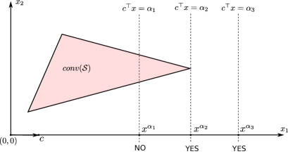
Figure 7: Reduction Example

Now, we consider IMDVP, for which the proofs take a similar approach.

Theorem 6.

The IMDVP is in ${\mathsf{NP}}$.

Proof.

The proof is almost identical to the proof that IMPVP is in ${\mathsf{coNP}}$. We show that there exists a short certificate that can validate the output YES. Let an instance $(\gamma,x^{0},c,A,b,r)$ of the IMDVP be given such that the output is YES. As in the proof of Theorem 4, it is enough to consider the case where $\gamma<\|c\|$ and we can assume without loss of generality that $\gamma>0$ (otherwise, the output is trivially YES). When the output is YES, by the characterization of Lemma 2, $\operatorname{int}\left(K(\gamma)\right)\cap\mathcal{C}^{\circ}(x^{0})=\emptyset$ holds and there exists $\overline{x}\in\operatorname{conv}(\mathcal{S}^{+})\cap\mathcal{K}^{*}(\gamma)$ with $\overline{x}\not=x^{0}$. As in the proof of Theorem 4, Carathéodory’s Theorem ensures there is a set of at most $n+1$ members of $\mathcal{S}^{+}$ whose convex combination yields $\overline{x}$ and this set of points is the short certificate. ∎

To show that IMDVP is complete for ${\mathsf{NP}}$, we need one more technical lemma, which exploits Proposition 1 to enable us to Karp-reduce MPVP to IMDVP. The basic idea is to exploit the property that the norm of the difference between two numbers can be bounded by a function of their encoding lengths. This allows us to cleanly distinguish the cases in which a given value is a primal bound for  (MILP) from that in which the given value is a strict dual bound by solving an IMDVP that we can can easily construct.

Lemma 3.

Let $\alpha\in\mathbb{Q}$ and let $\epsilon:=2^{-\max\{\langle c\rangle+\nu,\langle\alpha\rangle\}-1}$ and $\delta:=2^{-\langle x^{0}\rangle-\nu-1}$.

1. If $\alpha\leq\max_{x\in\mathcal{S}}c^{\top}x+\epsilon$, then $\alpha\leq\max_{x\in\mathcal{S}}c^{\top}x$.

2. If $\alpha\leq\max_{x\in\mathcal{S}}c^{\top}x$, then $\|c-d\|>\epsilon\delta>0$ for all $d\in\mathcal{C}^{\circ}(x^{\alpha-\epsilon})$, where $x^{\alpha-\epsilon}=(\alpha-\epsilon)\frac{c}{\|c\|^{2}_{2}}$.

Proof.

1. First, we have that the encoding length of $\max_{x\in\mathcal{S}}c^{\top}x$ is bounded by $\langle c\rangle+\nu$. Then if $\alpha>\max_{x\in\mathcal{S}}c^{\top}x$, $\alpha>\max_{x\in\mathcal{S}}c^{\top}x+\epsilon$ by Proposition 1. Therefore, $\alpha\leq\max_{x\in\mathcal{S}}c^{\top}x$.

2. Let $\alpha\leq\max_{x\in\mathcal{S}}c^{\top}x$ and $\overline{x}\in\operatorname{argmax}_{x\in\mathcal{S}}c^{\top}x$ be given such that $\overline{x}$ is an extreme point of $\operatorname{conv}(\mathcal{S})$ and let $x^{\alpha-\epsilon}:=(\alpha-\epsilon)\frac{c}{\|c\|^{2}_{2}}$. Since $c^{\top}\overline{x}\geq\alpha$ and $c^{\top}x^{\alpha-\epsilon}=\alpha-\epsilon<\alpha$, it follows that $\overline{x}\not=x^{\alpha-\epsilon}$. For an arbitrary $d\in\mathcal{C}^{\circ}(x^{\alpha-\epsilon})$, we have that

   $$d^{\top}(x^{\alpha-\epsilon}-\overline{x})\geq 0 \Leftrightarrow d^{\top}(x^{\alpha-\epsilon}-\overline{x})-c^{\top}(x^{\alpha-\epsilon}-\overline{x})+c^{\top}(x^{\alpha-\epsilon}-\overline{x})\geq 0$$

   $$\Leftrightarrow(d-c)^{\top}(x^{\alpha-\epsilon}-\overline{x})\geq c^{\top}\overline{x}-c^{\top}x^{\alpha-\epsilon}$$

   $$\Leftrightarrow(d-c)^{\top}(x^{\alpha-\epsilon}-\overline{x})\geq c^{\top}\overline{x}-\alpha+\epsilon$$ (3)

   $$\Leftrightarrow(d-c)^{\top}(x^{\alpha-\epsilon}-\overline{x})\geq\epsilon$$ (4)

   $$\Leftrightarrow\|c-d\|\|x^{\alpha-\epsilon}-\overline{x}\|\geq\epsilon$$ (5)

   $$\Leftrightarrow\|c-d\|\geq\frac{\epsilon}{\|x^{\alpha-\epsilon}-\overline{x}\|}$$ (6)

   $$\Leftrightarrow\|c-d\|>\epsilon\delta$$ (7)

   Equation (3) follows by substituting $(\alpha-\epsilon)\frac{c}{\|c\|_{2}^{2}}$ for $x^{\alpha-\epsilon}$; (4) follows from the nonnegativity of $c^{\top}\overline{x}-\alpha$; and (5) follows from the Cauchy–Schwarz inequality. Equation (6) follows from (5) because $\|\overline{x}-x^{\alpha-\epsilon}\|>0$. Equation (7) follows from the fact that ${\|x^{\alpha-\epsilon}-\overline{x}\|}<2^{\langle x^{\alpha-\epsilon}\rangle+\nu+1}$, again by Proposition 1, since the encoding length of $x^{\alpha-\epsilon}-\overline{x}$ is bounded by the vertex complexity $\nu$ of $\operatorname{conv}(\mathcal{S})$ and $\langle x^{\alpha-\epsilon}\rangle$.

∎

Theorem 7.

The IMDVP is complete for ${\mathsf{NP}}$.

Proof.

We show that the MPVP can be Karp-reduced to the IMDVP. Therefore, let an instance $(\alpha,c,A,b,r)$ of the MPVP be given and let $\epsilon$ and $\delta$ be given as in Lemma 3. Then we claim that the MPVP can be resolved by deciding the IMDVP with inputs $(\epsilon\delta,x^{\alpha-\epsilon},A,b,r)$, where $x^{\alpha-\epsilon}=(\alpha-\epsilon)\frac{c}{\|c\|^{2}_{2}}$. The IMDVP asks whether the set $\operatorname{int}\left(\mathcal{K}(\epsilon\delta)\right)\cap\mathcal{C}^{\circ}(x^{\alpha-\epsilon})$ is empty. Note that $c\in\operatorname{int}\left(\mathcal{K}(\epsilon\delta)\right)$. If the output to the IMDVP is YES, then $\operatorname{int}\left(\mathcal{K}(\epsilon\delta)\right)\cap\mathcal{C}^{\circ}(x^{\alpha-\epsilon})$ is empty. This means $c\not\in\mathcal{C}^{\circ}(x^{\alpha-\epsilon})$, i.e.,

$$c\notin\left\{d\in\mathbb{R}^{n}\mid d^{\top}\left(x-x^{\alpha-\epsilon}\right)\leq 0\;\forall x\in\mathcal{S}\right\}.$$

This in turn means that there exists an $\overline{x}\in\mathcal{S}$ such that

$$c^{\top}\left(\overline{x}-x^{\alpha-\epsilon}\right)>0 \Leftrightarrow c^{\top}\overline{x}-\alpha+\epsilon>0$$

$$\Leftrightarrow c^{\top}\overline{x}+\epsilon>\alpha$$

$$\Rightarrow c^{\top}\overline{x}\geq\alpha.$$

The last implication is by Lemma 3, part (i). Hence, the output to the MPVP is YES.

When the output to the IMDVP is NO, there exists $\hat{d}\in\operatorname{int}\left(\mathcal{K}(\epsilon\delta)\right)\cap\mathcal{C}^{\circ}(x^{\alpha-\epsilon})$. Then $\hat{d}\in\mathcal{C}^{\circ}(x^{\alpha-\epsilon})$ and $\|c-\hat{d}\|\leq\epsilon\delta$, so by the contraposition of Lemma 3, part (ii), there is no $\overline{x}\in\mathcal{S}$ such that $c^{\top}\overline{x}\geq\alpha$, i.e., $c^{\top}x<\alpha$ for all $x\in\mathcal{S}$. This means the output to the MPVP is NO. ∎

Figure 8a illustrates the case in which $c^{\top}x<\alpha_{3}$ holds for all $x\in\mathcal{S}$, so that the output of MPVP is NO. In this case, there exists $\hat{d}\in\operatorname{int}\left(\mathcal{K}(\epsilon\delta)\right)\cap\mathcal{C}^{\circ}(x^{\alpha-\epsilon})$. In fact, $c$ is itself in $\operatorname{int}\left(\mathcal{K}(\epsilon\delta)\right)\cap\mathcal{C}^{\circ}(x^{\alpha-\epsilon})$, which means the optimal value of the associated IMILP is 0. The instance of IMDVP specified in the reduction also has output NO, since we are checking the validity of a nonzero dual bound.

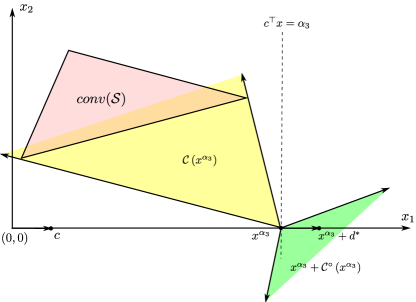
(a)

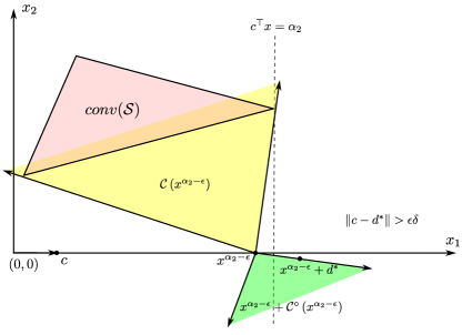
(b)

Figure 8: Lemma 3 on two simple examples

Figure 8b illustrates the case in which the optimal value to the MILP is exactly $\alpha_{2}$, so that the output of the MPVP is YES. In this case, Lemma 3 tells us that the optimal value for the associated IMILP must be greater than $\epsilon\delta$ and that the instance of IMDVP that we solve in the reduction must have output YES as well. Note the essential role of $\epsilon\delta$ as a number strictly between zero and the smallest possible positive optimal value that the associated instance of IMILP can have. This is necessary precisely because Lemma 2 does not hold for $\gamma=0$.

Theorem 8.

The IMOVP is complete for ${\mathsf{D}}^{{\mathsf{P}}}$.

Proof.

As noted before, the reduction presented in Theorem 7 can be used to reduce both the MDVP and the MPVP to the IMPVP and the IMDVP, respectively. Using this reduction, the language of the IMOVP can then be expressed as the intersection of the languages of the IMPVP and the IMDVP that are in ${\mathsf{coNP}}$ and ${\mathsf{NP}}$, respectively. This proves that the IMOVP is in class ${\mathsf{D}}^{{\mathsf{P}}}$. The IMOVP is complete for ${\mathsf{D}}^{{\mathsf{P}}}$, since the MOVP can be reduced to the IMOVP using the same reduction. ∎

Note that the optimal value verification problems associated with both the inverse and forward problems are complete for ${\mathsf{D}}^{{\mathsf{P}}}$, placing this decision version of both the forward and inverse problems in the same complexity class.

5 Conclusion and Future Directions

In this paper, we discussed the relationship of the inverse mixed integer linear optimization problem to both the associated forward and separation problems. We showed that the inverse problem can be seen as an optimization problem over the cone described by all inequalities valid for $\mathcal{S}$ and satisfied at equality by $x^{0}$ (the normal cone at $x^{0}$). Alternatively, it can also be seen as an optimization problem over the 1-polar under some additional assumptions. Both these characterizations make the connection with the separation problem associated with $\mathcal{S}$ evident.

By observing that the separation problem for the feasible region of the inverse problem under the $\ell_{1}$ and $\ell_{\infty}$ norms is an instance of the forward problem, it can be shown via a straightforward cutting-plane algorithm that the inverse problem can be solved by solving polynomially many instances of the forward problem with different objective functions. This is done by invoking the result of Grötschel et al. (1993), which shows that optimization and separation are polynomially equivalent, i.e., each can be Cook-reduced to the other. This in turn places the decision version of inverse MILP in the complexity class $\Delta_{2}^{p}$.

The main result of the paper is that a stronger analysis is possible. We first show that verification of a primal and dual bound for the inverse problem is in ${\mathsf{coNP}}$ and ${\mathsf{NP}}$ by providing short certificates for the NO and YES outputs, respectively. We show that verification of a dual bound for the forward problem can be Karp-reduced to verification of a primal bound for the associated inverse problem. Thus, both problems are complete for the class ${\mathsf{coNP}}$ and are on the same level of the polynomial-time hierarchy. Similarly, verification of a primal bound for the forward problem can be Karp-reduced to verification of a dual bound for the associated inverse problem. Thus, both of those problems are complete for the class ${\mathsf{NP}}$ and are also on the same level of the polynomial-time hierarchy. Finally, we use these two results to show that the verification problem for the optimal value of IMILP is complete for the class ${\mathsf{D}}^{{\mathsf{P}}}$, which is the same class that Papadimitriou and Yannakakis (1982) showed contains the MILP optimal value verification problem.

Although we have not done so formally, we believe the results in this paper lay the groundwork for stating some version of Theorem 1 that incorporates the equivalence of the inverse problem and is stated in terms of Karp reduction. The form such a result would take is not entirely obvious. Whereas the essence of the separation problem is to determine whether or not a given point is a member of a given convex set, the inverse problem implicitly demands that we determine which of three sets contains a given point: the relative interior of a given convex set, the boundary of that convex set, or the complement of the set. Whereas it is known that the problem of determining whether or not a given point is contained in the convex hull of solutions is complete for ${\mathsf{NP}}$, our results indicate that the related problem of determining if a given point is on the boundary of the feasible set of an MILP is a complete problem for ${\mathsf{D}}^{{\mathsf{P}}}$, while the problems of determining whether a given point is contained in the convex hull of solutions or determining whether a given point is contained in the complement of the relative interior are in ${\mathsf{NP}}$ and ${\mathsf{coNP}}$, respectively. Given all of this, it seems clear that a unified result integrating all of the various problems we have introduced and stating their equivalence in terms of Karp reduction should be possible.

Finally, while we have implemented the cutting-plane algorithm in this paper, it is clear that more work must be done to develop computationally efficient algorithms for solving the inverse versions of difficult combinatorial optimization problems. Development of customized algorithms for which the number of oracle calls required in practice can be reduced is a next natural step. Given our results, the existence of a direct algorithm for solving inverse problems can also not be ruled out.

References

- Aaronson [2017] S. Aaronson. P NP. Technical report, University of Texas at Austin, 2017. URL https://www.scottaaronson.com/papers/pnp.pdf.
- Ahuja and Orlin [2001] Ravindra K. Ahuja and James B. Orlin. Inverse optimization. Operations Research, 49(5):771–783, 2001. doi: 10.1287/opre.49.5.771.10607.
- Arora and Barak [2007] S. Arora and B. Barak. Computational Complexity: A Modern Approach. Cambridge University Press, 2007.
- Beigel and Fortnow [2003] R. Beigel and L. Fortnow. Are cook and karp ever the same? In Proceedings of the Annual IEEE Conference on Computational Complexity, pages 333–336, 2003.
- Boyd [1994] E. Andrew Boyd. Fenchel cutting planes for integer programs. Operations Research, 42(1):53–64, 1994. doi: 10.1287/opre.42.1.53. URL http://dx.doi.org/10.1287/opre.42.1.53.
- Cai et al. [1999] M. C. Cai, X. G. Yang, and J. Z. Zhang. The complexity analysis of the inverse center location problem. Journal of Global Optimization, 15(2):213–218, September 1999. ISSN 1573-2916. doi: 10.1023/A:1008360312607. URL https://doi.org/10.1023/A:1008360312607.
- Cook [1971] Stephen A. Cook. The complexity of theorem-proving procedures. In Proceedings of the Third Annual ACM Symposium on Theory of Computing, STOC ’71, pages 151–158, New York, NY, USA, 1971. ACM. doi: 10.1145/800157.805047. URL http://doi.acm.org/10.1145/800157.805047.
- Edmonds [1971] Jack Edmonds. Matroids and the greedy algorithm. Mathematical programming, 1(1):127–136, 1971.
- Garey and Johnson [1979] Michael R. Garey and David S. Johnson. Computers and Intractability: A Guide to the Theory of NP-Completeness. W. H. Freeman & Co., New York, NY, USA, 1979. ISBN 0716710447.
- Grötschel et al. [1993] M. Grötschel, L. Lovász, and A. Schrijver. Geometric Algorithms and Combinatorial Optimization. Algorithms and Combinatorics. Springer, second corrected edition edition, 1993.
- Heuberger [2004] Clemens Heuberger. Inverse combinatorial optimization: a survey on problems, methods, and results. Journal of Combinatorial Optimization, 8(3):329–361, September 2004. ISSN 1573-2886. doi: 10.1023/B:JOCO.0000038914.26975.9b. URL https://doi.org/10.1023/B:JOCO.0000038914.26975.9b.
- Huang [2005] Siming Huang. Inverse problems of some NP-complete problems, pages 422–426. Springer Berlin Heidelberg, Berlin, Heidelberg, 2005. ISBN 978-3-540-32440-9. URL https://doi.org/10.1007/11496199_45.
- Karp [1972] Richard M Karp. Reducibility among combinatorial problems. In Complexity of computer computations, pages 85–103. Springer, 1972.
- Krentel [1988] Mark W. Krentel. The complexity of optimization problems. Journal of Computer and System Sciences, 36(3):490 – 509, 1988. ISSN 0022-0000. doi: https://doi.org/10.1016/0022-0000(88)90039-6. URL http://www.sciencedirect.com/science/article/pii/0022000088900396.
- Krentel [1987a] Mark William Krentel. The Complexity of Optimization Problems. PhD thesis, Cornell University, Ithaca, New York, May 1987a.
- Krentel [1987b] M.W. Krentel. The Complexity of Optimization Problems. PhD thesis, Cornell University, 1987b.
- Lutz and Mayordomo [1995] J.H. Lutz and E. Mayordomo. Cook versus karp-levin: Separating completeness notions if np is not small. Theoretical Computer Science, 164:141–163, 1995.
- Papadimitriou and Yannakakis [1982] C. H. Papadimitriou and M. Yannakakis. The complexity of facets (and some facets of complexity). In Proceedings of the fourteenth annual ACM symposium on Theory of computing, STOC ’82, pages 255–260, New York, NY, USA, 1982. ACM. ISBN 0-89791-070-2. doi: 10.1145/800070.802199. URL http://doi.acm.org/10.1145/800070.802199.
- Papadimitriou [1981] C.H. Papadimitriou. On the complexity of integer programming. Journal of the Association for Computing Machinery, 28:765–768, 1981.
- Papadimitriou [2003] Christos H. Papadimitriou. Computational complexity. In Encyclopedia of Computer Science, pages 260–265. John Wiley and Sons Ltd., Chichester, UK, 2003. ISBN 0-470-86412-5. URL http://dl.acm.org/citation.cfm?id=1074100.1074233.
- Rockafellar [1970] R. T. Rockafellar. Convex Analysis. Princeton University Press, 1970.
- Schaefer [2009] Andrew J. Schaefer. Inverse integer programming. Optimization Letters, 3(4):483–489, September 2009. ISSN 1862-4480. doi: 10.1007/s11590-009-0131-z. URL https://doi.org/10.1007/s11590-009-0131-z.
- Schrijver [1986] Alexander Schrijver. Theory of integer and linear programming. Wiley, Chichester, 1986.
- Stockmeyer [1976a] L.J. Stockmeyer. The polynomial-time hierarchy. Theoretical Computer Science, 3(1):1 – 22, 1976a. ISSN 0304-3975. doi: https://doi.org/10.1016/0304-3975(76)90061-X. URL http://www.sciencedirect.com/science/article/pii/030439757690061X.
- Stockmeyer [1976b] L.J. Stockmeyer. The polynomial-time hierarchy. Theoretical Computer Science, 3:1–22, 1976b.
- Turing [1937] Alan M Turing. On computable numbers, with an application to the entscheidungsproblem. Proceedings of the London mathematical society, 2(1):230–265, 1937.
- Vollmer and Wagner [1995] H. Vollmer and K.W. Wagner. Complexity classes of optimization functions. Information and Computation, 120(2):198 – 219, 1995. ISSN 0890-5401. doi: https://doi.org/10.1006/inco.1995.1109. URL http://www.sciencedirect.com/science/article/pii/S0890540185711091.
- Wang [2009] Lizhi Wang. Cutting plane algorithms for the inverse mixed integer linear programming problem. Operations Research Letters, 37(2):114 – 116, 2009. ISSN 0167-6377. doi: http://dx.doi.org/10.1016/j.orl.2008.12.001. URL http://www.sciencedirect.com/science/article/pii/S0167637708001326.