\DoubleSpacedXI\TheoremsNumberedThrough\ECRepeatTheorems\EquationsNumberedThrough
\RUNTITLE

Transfer Learning of Word Embeddings

\TITLE

Group-Sparse Matrix Factorization for Transfer Learning of Word Embeddings

\ARTICLEAUTHORS\AUTHOR

Kan Xu \AFFUniversity of Pennsylvania, Economics, \EMAILkanxu@sas.upenn.edu \AUTHORXuanyi Zhao \AFFUniversity of Pennsylvania, Computer and Information Science, \EMAILxuanyi.zhao@hotmail.com \AUTHORHamsa Bastani \AFFWharton School, Operations Information and Decisions, \EMAILhamsab@wharton.upenn.edu \AUTHOROsbert Bastani \AFFUniversity of Pennsylvania, Computer and Information Science, \EMAILobastani@seas.upenn.edu

\ABSTRACT

Unstructured text provides decision-makers with a rich data source in many domains, ranging from product reviews in retailing to nursing notes in healthcare. To leverage this information, words are typically translated into word embeddings—vectors that encode the semantic relationships between words—through unsupervised learning algorithms such as matrix factorization. However, learning word embeddings from new domains with limited training data can be challenging, because the meaning/usage may be different in the new domain, e.g., the word “positive” typically has positive sentiment, but often has negative sentiment in medical notes since it may imply that a patient is tested positive for a disease. Intuitively, we expect that only a small number of domain-specific words may have new meanings/usages. We propose an intuitive two-stage estimator that exploits this structure via a group-sparse penalty to efficiently transfer learn domain-specific word embeddings by combining large-scale text corpora (such as Wikipedia) with limited domain-specific text data. We bound the generalization error of our estimator, proving that it can achieve the same accuracy (compared to not transfer learning) with substantially less domain-specific data when only a small number of embeddings are altered between domains. Our results provide the first bounds on group-sparse matrix factorization, which may be of independent interest. We empirically evaluate the effectiveness of our approach compared to state-of-the-art fine-tuning heuristics from natural language processing.

\KEYWORDS

word embeddings, transfer learning, group sparsity, matrix factorization, text analytics, natural language processing

1 Introduction

Natural language processing is an increasingly important part of the analytics toolkit for leveraging unstructured text data in a variety of domains. For instance, service providers mine online consumer reviews to inform operational decisions on platforms (Mankad et al. 2016) or to infer market structure and the competitive landscape for products (Netzer et al. 2012); Twitter posts are used to forecast TV show viewership (Liu et al. 2016); analyst reports of S&P 500 firms are used to measure innovation (Bellstam et al. 2020); medical notes are used to predict operational metrics such as readmissions rates (Hsu et al. 2020); online ads or reviews are used to flag service providers that are likely engaging in illicit activities (Ramchandani et al. 2021, Li et al. 2021).

To leverage unstructured text in decision-making, we must preprocess the text to capture the semantic content of words in a way that can be passed as an input to a predictive machine learning algorithm. In the past, this involved domain experts performing costly and imperfect feature engineering. A much more powerful, data-driven approach is to use unsupervised learning algorithms to learn word embeddings, which represent words as vectors (Mikolov et al. 2013, Pennington et al. 2014); we focus on widely-used word embedding models that are based on low-rank matrix factorization (Pennington et al. 2014, Levy and Goldberg 2014). These word embeddings translate semantic similarities between words and the context within which they appear into statistical relationships. Typically, they are trained to encode how frequently pairs of words co-occur in text; these co-occurrence counts implicitly contain semantic properties of words since words with similar meanings tend to occur in similar contexts. Given the large number of words in the English language, to be effective in practice, embeddings must be trained on large-scale and comprehensive text data, e.g., popular embeddings such as Word2Vec (Mikolov et al. 2013) and GloVe (Pennington et al. 2014) are trained on Wikipedia articles.

However, it is well-known that pre-trained word embeddings can miss out on important domain-specific meaning/usage, hurting downstream interpretations and predictive accuracy. For example, the word “positive” is typically associated with positive sentiment on Wikipedia; yet, in the context of medical notes, it typically indicates the presence of a medical condition, corresponding to negative sentiment. Thus, using a generic word embedding for “positive” may diminish performance in medical applications. Similarly, words like “adherence” (referring to medication adherence) have a specific meaning in a healthcare context (relative to its context on general Wikipedia entries) and are strongly predictive of patient outcomes; failing to account for its healthcare-specific meaning may result in a loss in the downstream accuracy of healthcare-specific prediction tasks (Blitzer et al. 2007). Consequently, there has been a large body of work training specialized embeddings in a number of diverse contexts ranging from radiology reports (Ong et al. 2020), cybersecurity vulnerability reports (Roy et al. 2017), and patent classification (Risch and Krestel 2019). This approach only works when the decision-maker has access to a sufficiently large domain-specific text corpus, allowing her to train high-quality embeddings. In practice, decision-makers often have limited domain-specific text data, yielding poor results when training new word embeddings, which hurts the quality of downstream modeling and decisions that leverage these embeddings. In other words, word embeddings trained on domain-specific data alone are unbiased but can have high variance due to limited sample size; in contrast, pre-trained word embeddings have low variance but can be significantly biased depending on the extent of domain mismatch.

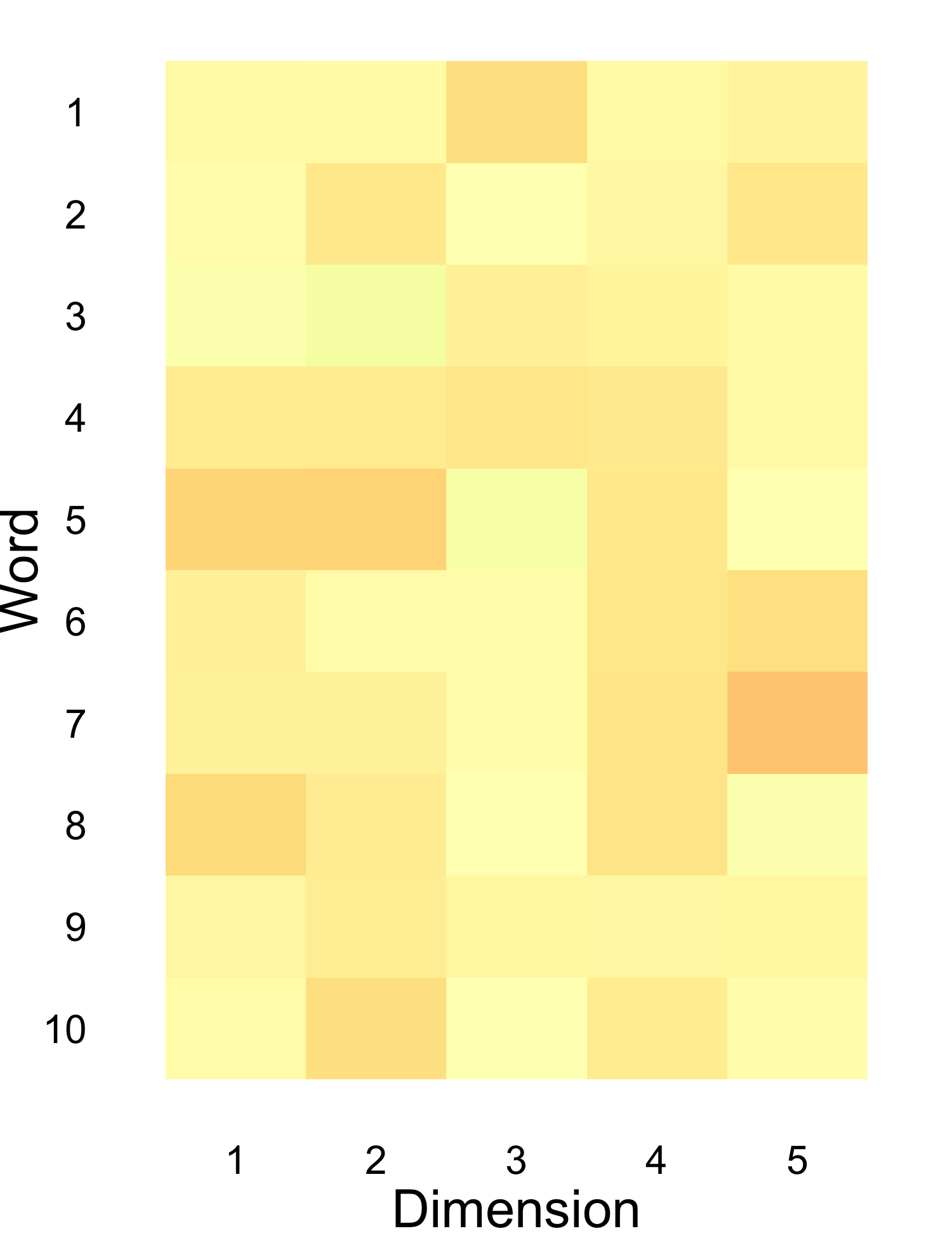
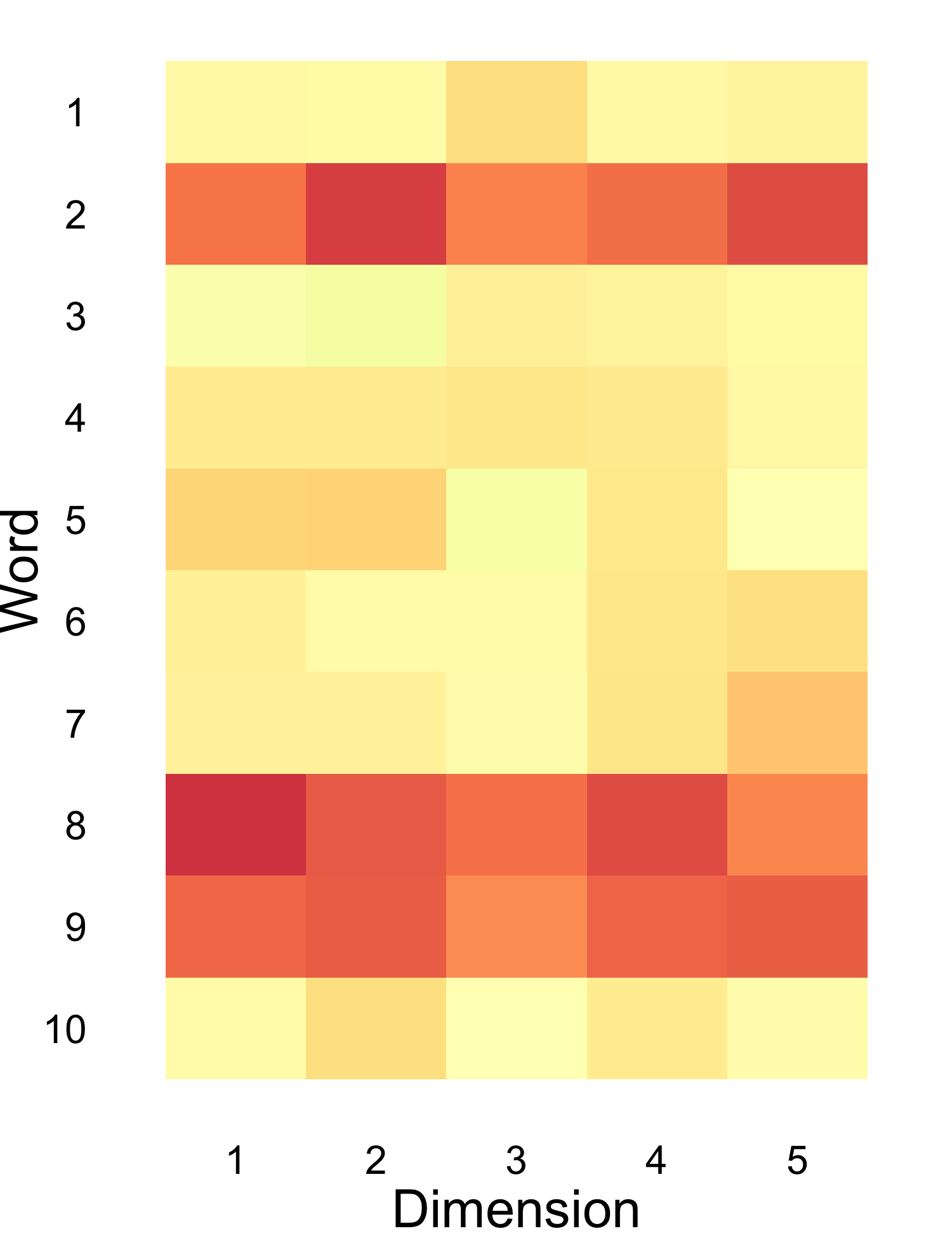
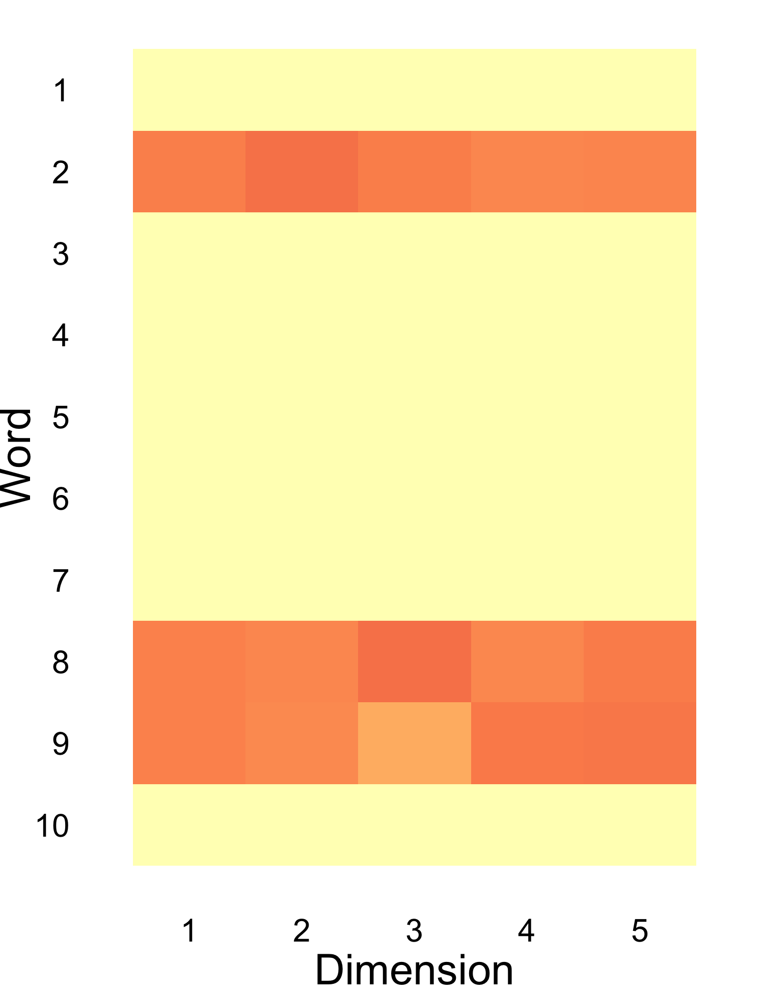
Then, a natural question is whether we can combine large-scale publicly available text corpora (which we call the proxy data hereafter) with limited domain-specific text data (which we call the gold data hereafter) to train precise but domain-specific word embeddings. In particular, we aim to use transfer learning to achieve a better bias-variance tradeoff than using gold or proxy data alone. Our key insight to enable transfer learning is that the meaning/usage of most words do not change when changing domains; rather, we expect that only a small number of domain-specific words will have new meaning/usage. More formally, consider a corpus of $d$ words. Let $U_{p}\in\mathbb{R}^{d\times r}$ denote the true (unobserved) proxy word embedding matrix, of which the $i^{\text{th}}$ row $U_{p}^{i}$ is the true $r$-dimensional word embedding of word $i\in[d]=\{1,\cdots,d\}$ based on the proxy data; analogously, let $U_{g}\in\mathbb{R}^{d\times r}$ denote the true (unobserved) gold word embedding matrix. We expect that the meaning/usage for most words are preserved in both domains—i.e., the word embeddings $U_{g}^{i}=U_{p}^{i}$ for most $i\in[d]$. This induces a group-sparse structure for the difference matrix $U_{g}-U_{p}$, i.e., only a small number of rows (groups) are nonzero. Figure 1 illustrates this notion of “sparsity” on a toy example with $d=10$ words, embeddings with dimension $r=5$, and $s=3$ words with shifted meaning/usage.

Refer to caption
\alphalph $U_{p}$
Refer to caption
\alphalph $U_{g}$
Refer to caption
\alphalph $U_{g}-U_{p}$
Figure 1: Toy example of (a) proxy and (b) gold word embedding matrices for $d=10$ and $r=5$. Only $s=3$ words change meaning/usage, inducing a group-sparse structure in the (c) difference matrix.

Based on this intuition, we formulate an objective that incorporates a group-sparse penalty (Friedman et al. 2010, Simon et al. 2013) on $U_{g}-U_{p}$, where each row is treated as a group. In particular, we estimate domain-specific embeddings from gold data, incorporating $\ell_{2,1}$ regularization to impose group sparsity relative to the (estimated) word embeddings trained on the large proxy data. Our approach balances the need to update the embeddings of important domain-specific words based on the gold data (i.e., reduce bias), while matching most words to the embeddings estimated from the large proxy text corpus (i.e., reduce variance).

Our main result establishes that the word embedding estimator trained by group-sparse transfer learning achieves a sample complexity bound that scales linearly with the number of words, as opposed to the conventional quadratic scaling. In other words, transfer learning allows us to accurately identify domain-specific word embeddings with substantially less domain-specific data than classical low-rank matrix factorization methods. We build on prior work establishing error bounds for the group LASSO (Lounici et al. 2011) and low-rank matrix problems (Ge et al. 2017, Negahban and Wainwright 2011). We face two additional technical challenges. First, the literature on nonconvex low-rank matrix problems typically studies the Hessian to ensure that local minima are well-behaved; however, the Hessian may not be well-defined under our non-smooth group-sparse penalty (since the gradient is not continuous). Second, unlike the traditional high-dimensional literature, transfer learning introduces a quartic form (in terms of $U_{g}-U_{p}$) in our objective function. We address both challenges through a new analysis that relies on an assumption we term “quadratic compatibility condition.” We show that quadratic compatibility is implied by a natural restricted strong convexity (RSC) assumption; furthermore, under a slightly stronger RSC condition from Loh and Wainwright (2015), all local minima identified by our algorithm are statistically indistinguishable from the global minimum.

While our technical results hold for embeddings trained using matrix factorization, our algorithm straightforwardly applies to nonlinear objectives such as GloVe. Simulations on synthetic data show that our estimator significantly outperforms common heuristics given rich proxy data and limited domain-specific data. Importantly, we show that this is an interpretable strategy to identifying key words with distinct meanings in specific domains such as finance, math, and computing. We also demonstrate the efficacy of our approach in a downstream prediction task of clinical trial eligibility based on unstructured clinical statements regarding inclusion or exclusion criteria.

1.1 Related Literature

Transfer learning involves transferring knowledge from a data-rich source domain to a data-poor target domain (also called “domain adaptation”). In order for such approaches to be effective, the two domains must be related in some way. For instance, the two domains may have the same label distribution $p(y\mid x)$ but different covariate distributions $p(x)$, a setting typically termed as “covariate shift” (see, e.g., Ben-David et al. 2007, 2010, Ganin and Lempitsky 2015). Our problem falls into the more challenging category known as “label shift,” where $p(y\mid x)$ itself differs across the two domains (since the underlying embeddings change for some words). A number of approaches have been proposed for addressing label shift in supervised learning problems (see, e.g., Lipton et al. 2018, Zhang et al. 2013).111Problems with labeled source data and unlabeled target data are sometimes referred to as “unsupervised”; we categorize them as “supervised” to distinguish from problems where both source and target data are unlabeled. Our approach is most closely related to recent work applying LASSO for transfer learning (Bastani 2020), where the label shift is driven by a sparse shift in the underlying parameter vectors. Their key theoretical result is that relative sparsity between the gold and proxy parameter vectors is sufficient to enable efficient transfer learning in high dimensions. Existing theoretical results are critically limited to supervised learning. To the best of our knowledge, we propose the first framework for theoretically understanding the value of transfer learning in natural language processing (generally considered an unsupervised learning problem), which introduces new technical challenges.

However, a number of practical heuristics have been proposed for domain adaptation for natural language processing. A surprisingly effective transfer learning strategy is to simply fine-tune pre-trained word embeddings on data from the target domain. Intuitively, stochastic gradient descent has regularization properties similar to $\ell_{2}$ regularization (Ali et al. 2020), so this strategy can be interpreted as regularizing the target word embeddings towards towards the pre-trained word embeddings (Dingwall and Potts 2018, Yang et al. 2017). We demonstrate empirically that our approach of using $\ell_{1}$ regularization outperforms these heuristics in the low-data regime.

We build on approaches that construct word embeddings based on low-rank matrix factorization (Pennington et al. 2014, Levy and Goldberg 2014). Levy and Goldberg (2014) show that one popular approach—skip-gram with negative sampling—implicitly factorizes a word-context matrix shifted by a global constant. Another popular approach is GloVe (Pennington et al. 2014), which uses a nonlinear version of our loss function; our estimator extends straightforwardly to this setting.

Accordingly, we build on the theoretical literature on low-rank matrix factorization—specifically the Burer-Monteiro approach (Burer and Monteiro 2003), which replaces $\Theta$ with a low-rank representation $UU^{T}$, with $U\in\mathbb{R}^{d\times r}$, and minimizes the objective in $U$. Ge et al. (2017) shows that the local minima of this nonconvex problem are also global minima under the restricted isometry property; Li et al. (2019) extend this by considering a more general objective function that satisfies a restricted well-conditioned assumption. One alternative is the nuclear-norm regularization (Recht et al. 2007, Candes and Plan 2011, Negahban and Wainwright 2011), but this algorithm lends less naturally to our transfer learning objective and is often computationally inefficient.

In addition to substantially expanding on the technical intuition and discussion, this paper extends our short conference paper (Xu et al. 2021) as follows. First, we show that the quadratic compatibility condition (a critical component of our proofs) is implied by a natural restricted strong convexity condition, which we prove holds with high probability for the illustrative case of Gaussian data (§2.4). Second, we prove that all local minima identified by our estimator are statistically indistinguishable from the global minimum under a slightly stronger condition by Loh and Wainwright (2015)3.3). Finally, we relate our error bounds back to the natural parameter scaling specific to word embedding models (§3.4).

2 Problem Formulation

We first formalize the problem of learning word embeddings as a low-rank matrix sensing problem (§2.1), and describe our transfer learning approach (§2.2). We then state our assumptions (§2.3) and provide intuition for our quadratic compatibility condition (§2.4).

Notation. For any vector $v\in\mathbb{R}^{d}$, let $\|v\|$ denote its $\ell_{2}$ norm. For a matrix $\Theta\in\mathbb{R}^{d_{1}\times d_{2}}$ of rank $r$, we denote its singular values by $\sigma_{\max}(\Theta)=\sigma_{1}(\Theta)\geq\sigma_{2}(\Theta)\geq\cdots\geq\sigma_{r}(\Theta)=\sigma_{\min}(\Theta)>0$, its Frobenius norm by $\|\Theta\|_{F}=\sqrt{\sum_{j=1}^{r}\sigma_{j}^{2}(\Theta)}$, its operator norm by $\|\Theta\|=\sigma_{1}(\Theta)$, its vector $\ell_{\infty}$ norm by $|\Theta|_{\infty}=\max_{i,j}|\Theta_{ij}|$, its vector $\ell_{1}$ norm by $|\Theta|_{1}=\sum_{i,j}|\Theta_{ij}|$, and its matrix $\ell_{2,1}$ norm by $\|\Theta\|_{2,1}=\sum_{j=1}^{d_{1}}\|\Theta^{j}\|$, where $\Theta_{ij}$ represents entry $(i,j)$ of $\Theta$ and $\Theta^{j}$ the $j^{\text{th}}$ row of $\Theta$. Given $\Theta,\Theta^{\prime}\in\mathbb{R}^{d_{1}\times d_{2}}$, we denote the matrix dot product by $\langle\Theta,\Theta^{\prime}\rangle=\sum_{i=1}^{d_{1}}\sum_{j=1}^{d_{2}}\Theta_{ij}\Theta^{\prime}_{ij}$. Finally, let $[k]=\{1,2,\cdots,k\}$.

2.1 Matrix Sensing

Our word embedding model is an instance of the more general setting of matrix sensing (Recht et al. 2007), where one aims to recover an unknown symmetric matrix $\Theta^{*}\in\mathbb{R}^{d\times d}$ with rank $r\ll d$. In other words, we can write $\Theta^{*}=U^{*}U^{*T}$ where $U^{*}\in\mathbb{R}^{d\times r}$. The typical goal in matrix sensing is to estimate $\Theta^{*}$ given observations $A_{i}\in\mathbb{R}^{d\times d}$ and $X_{i}\in\mathbb{R}$, for $i\in[n]$, where

$\displaystyle X_{i}=\langle A_{i},\Theta^{*}\rangle+\epsilon_{i},$ (1)

and $\epsilon_{1},\cdots,\epsilon_{n}$ are independent $\sigma$-subgaussian random variables (Definition 2.1). To simplify notation, we define the linear operator $\mathcal{A}:\mathbb{R}^{d\times d}\to\mathbb{R}^{n}$, where $\mathcal{A}(\Theta)_{i}=\langle A_{i},\Theta\rangle$. Then, we can write

$\displaystyle X=\mathcal{A}(\Theta^{*})+\epsilon,$

where $X=[X_{1},\cdots,X_{n}]^{T}$ and $\epsilon=[\epsilon_{1},\cdots,\epsilon_{n}]^{T}$.

Definition 2.1

A random variable $z$ is $\sigma$-subgaussian if, for any $t\in\mathbb{R}$, $\mathbb{E}[\exp(tz)]\leq\exp(t^{2}\sigma^{2}/2)$.

As we will discuss at the end of this subsection, in natural language processing, $\Theta^{*}$ corresponds to the word co-occurrence probability matrix, while $U^{*}$ corresponds to the word embeddings. Thus, in contrast to the matrix sensing literature which aims to estimate $\Theta^{*}$, our goal is to estimate the low-rank representation $U^{*}$. However, we can only compute $U^{*}$ up to an orthogonal change-of-basis since $\Theta^{*}$ is preserved under such a transformation—i.e., if we let $\widetilde{U}^{*}=U^{*}R$ for an orthogonal matrix $R\in\mathbb{R}^{r\times r}$, then we still obtain $\widetilde{U}^{*}\widetilde{U}^{*T}=U^{*}RR^{T}U^{*T}=U^{*}U^{*T}=\Theta^{*}$. Thus, our goal is to compute $\widehat{U}$ such that $\widehat{U}\approx U^{*}R$ for some orthogonal matrix $R$.

We build on Burer and Monteiro (2003), which solves the following optimization problem:

$\displaystyle\min_{U\in\mathbb{R}^{d\times r}}\frac{1}{n}\|X-\mathcal{A}(UU^{T})\|^{2}.$

Despite its nonconvex loss, this estimator performs well in practice, and has desirable theoretical properties (i.e., no spurious local minima) under the restricted isometry property (Ge et al. 2017).

We measure the estimation error of $\widehat{U}$ using the $\ell_{2,1}$ norm, which is more compatible with the group-sparse structure that we will impose shortly. In addition, since we can only identify $U^{*}$ up to orthogonal change-of-basis, we consider the following rotation-invariant error.

Definition 2.2

Given $\widehat{U},U^{*}\in\mathbb{R}^{d\times r}$, the error of $\widehat{U}$ is

$\displaystyle\ell(\widehat{U},U^{*})$ $\displaystyle=\|\widehat{U}-U^{*}R_{(\widehat{U},U^{*})}\|_{2,1},$

where $R_{(\widehat{U},U^{*})}=\argmin_{R:R^{T}R=RR^{T}=\mathbf{I}}\|\widehat{U}-U^{*}R\|_{F}$.

Remark 2.3

An alternative approach to Burer-Monteiro is to estimate $\Theta^{*}$ directly using nuclear norm regularization (see, e.g., Candes and Plan 2011, Negahban and Wainwright 2011). However, this approach is often too computationally costly in large-scale problems (Recht et al. 2007). Furthermore, estimating $U^{*}$ is more natural in our setting since our final goal is to recover $U^{*}$ (rather than $\Theta^{*}$), and our transfer learning strategy penalizes deviations in $U^{*}$.

Word embeddings. Word embedding models typically consider how often pairs of words co-occur within a fixed-length window. Without loss of generality, we consider neighboring word pairs, i.e., a window with length 1. Let the length of our text corpus be $n+1$ so that the total number of neighboring word pairs is $n$. Recall that we have $d$ unique words, and we define our word co-occurrence matrix $\Theta^{*}\in\mathbb{R}^{d\times d}$ such that the entry $\Theta^{*}_{jk}$ is the probability that word $j$ and word $k$ appear together. To estimate these probabilities, for each of the $d^{2}$ possible word pairs $(j,k)$, we randomly draw $n$ word pairs from the text (with replacement) and record our outcome as the binary indicator for whether the draw matched the pair $(j,k)$. This yields $d^{2}n$ samples, and for each $i\in[d^{2}n]$, our observation model is of the form

$\displaystyle X_{i}=\langle A_{i},\Theta^{*}\rangle+\epsilon_{i},$ (2)

where $A_{i}$ is a basis matrix and $X_{i}$ is a Bernoulli random variable. In particular, when entry $(j,k)$ of $A_{i}$ equals 1, $X_{i}$ equals 1 if the sampled word pair is $(j,k)$ and 0 otherwise. We discuss how our general results scale under this word embedding model in §3.4.

2.2 Transfer Learning

We now consider transfer learning from a large text corpus to the desired target domain. Let $U_{p}^{*}\in\mathbb{R}^{d\times r}$ denote the unknown word embeddings from the proxy (source) domain, and $U_{g}^{*}\in\mathbb{R}^{d\times r}$ denote the unknown word embeddings from the gold (target) domain. Our goal is to use data from both domains to estimate $U_{g}^{*}$ (up to rotations). In particular, we are given proxy data $\mathcal{A}_{p}:\mathbb{R}^{d\times d}\to\mathbb{R}^{n_{p}}$ and $X_{p}\in\mathbb{R}^{n_{p}}$ from the source domain, along with gold data $\mathcal{A}_{g}:\mathbb{R}^{d\times d}\to\mathbb{R}^{n_{g}}$ and $X_{g}\in\mathbb{R}^{n_{g}}$ from the target domain, such that

$\displaystyle X_{p}$ $\displaystyle=\mathcal{A}_{p}(\Theta_{p}^{*})+\epsilon_{p}\quad\text{and}\quad X_{g}=\mathcal{A}_{g}(\Theta_{g}^{*})+\epsilon_{g},$

where $\epsilon_{p}\in\mathbb{R}^{n_{p}}$ and $\epsilon_{g}\in\mathbb{R}^{n_{g}}$ are independent $\sigma_{p}$- and $\sigma_{g}$-subgaussian random variables respectively.

We are interested in the setting where $(n_{g}/\sigma_{g}^{2})\ll(n_{p}/\sigma_{p}^{2})$. As we will discuss later, this regime holds when we have limited domain-specific data but a large text corpus from other domains.

Group-Sparse Structure. To enable transfer learning, we must assume some relationship between the proxy and gold domains. Motivated by our previous discussion, we assume that

$$\Delta_{U}^{*}=U_{g}^{*}-U_{p}^{*},$$

has a row-sparse structure—i.e., most of its rows are 0. This structure arises when the embeddings of most words are preserved across domains, but a few words have a different meaning/usage in the new domains (see illustration in Figure 1\alphalph). More precisely, let the index set

$\displaystyle J=\left\{j\in[d]\Bigm{|}\|\Delta_{U}^{*j}\|\neq 0\right\},$

correspond to the set of rows with nonzero entries. The group sparsity of $\Delta_{U}^{*}$ is $s=|J|$. Then, a high-quality estimate of $U_{p}^{*}$ (from the large text corpus) can help us recover $U_{g}^{*}$ with less data, since the sample complexity of estimating $\Delta_{U}^{*}$ (due to its sparse structure) is less than that of $U_{g}^{*}$.

Note that the row-sparse structure of $\Delta_{U}^{*}$ is preserved under orthogonal transformations that are applied to both $U_{g}^{*}$ and $U_{p}^{*}$—i.e., if $\widetilde{U}_{p}^{*}=U_{p}^{*}R$ and $\widetilde{U}_{g}^{*}=U_{g}^{*}R$ for an orthogonal matrix $R$, then $\widetilde{\Delta}_{U}^{*}=\widetilde{U}_{g}^{*}-\widetilde{U}_{p}^{*}=(U_{g}^{*}-U_{p}^{*})R=\Delta_{U}^{*}R$ has the same group sparsity as $\Delta_{U}^{*}$.

2.3 Assumptions

We make two assumptions on the proxy and gold linear operators. Our first assumption is a standard restricted well-conditionedness (RWC) property on $\mathcal{A}_{p}$ from the matrix factorization literature (Li et al. 2019), which allows us to recover high-quality estimates of the proxy word embeddings $U_{p}^{*}$. Our second assumption is a quadratic compatibility condition (QCC) on $\mathcal{A}_{g}$, which allows us to recover $U_{g}^{*}$ despite our non-smooth and quartic objective function.

Definition 2.4

A linear operator $\mathcal{A}$ satisfies the $r$-RWC$(\alpha,\beta)$ condition if

$$\alpha\|Z\|_{F}^{2}\leq\frac{1}{n}\|\mathcal{A}(Z)\|^{2}\leq\beta\|Z\|_{F}^{2},$$

with $3\alpha>2\beta$ and for any $Z\in\mathbb{R}^{d\times d}$ with $\operatorname{rank}(Z)\leq r$.

This property is a generalization of the standard restricted isometry property (RIP). Under RIP, low-rank matrix problems have no spurious local minima—i.e., they are all global minima (Bhojanapalli et al. 2016, Park et al. 2017, Ge et al. 2017). However, RIP is very restrictive as it requires all the eigenvalues of the Hessian matrix to be within a small range of 1. The RWC condition applies more generally and guarantees statistical consistency for all local minima (Li et al. 2019). {assumption} The proxy linear operator $\mathcal{A}_{p}$ satisfies $2r$-RWC$(\alpha_{p},\beta_{p})$. Our first assumption is mild since we have a large proxy dataset, i.e., $n_{p}\gg d^{2}$. The degree of freedom of a $d\times d$ matrix $Z$ of rank $r$ is $r(2d-r)$; thus, in general, we only require $n\geq r(2d-r)$ observations to achieve the lower bound in Definition 2.4. For instance, when $\mathcal{A}$ is a Gaussian ensemble, RIP holds with high probability when $n\gtrsim dr$ (Candes and Plan 2011, Recht et al. 2007).

Definition 2.5 (QCC)

A linear operator $\mathcal{A}$ satisfies the quadratic compatibility condition with matrix $U^{*}$ and constant $\kappa$ (QCC$(U^{*},\kappa)$) if

$\displaystyle\frac{1}{n}\|\mathcal{A}(\Delta U^{*T}+U^{*}\Delta^{T}+\Delta\Delta^{T})\|^{2}\geq\frac{\kappa}{s}\left(\sum_{j\in J}\|\Delta^{j}\|\right)^{2}$

for any $\Delta\in\mathbb{R}^{d\times r}$ that satisfies $\sum_{j\in J^{c}}\|\Delta^{j}\|\leq 7\sum_{j\in J}\|\Delta^{j}\|$.

Compared to the standard compatibility condition in the group-sparse setting (Lounici et al. 2011), QCC includes an extra quadratic term $\Delta\Delta^{T}$ on the left hand side for nonconvex matrix factorization. We give a detailed discussion of this condition in the next subsection. {assumption} The gold linear operator $\mathcal{A}_{g}$ satisfies QCC$(U_{g}^{*},\kappa)$.

2.4 Quadratic Compatibility Condition

We now bridge QCC (Definition 2.5) with a restricted strong convexity (RSC) condition that is adapted to our setting; such conditions are common in the high-dimensional literature. We prove that RSC holds in our setting with high probability for the illustrative case of Gaussian data.

Definition 2.6 (RSC)

The operator $\mathcal{A}$ satisfies the restricted strong convexity with matrix $U^{*}$ and constant $\eta,\tau$ (RSC$(U^{*},\eta,\tau)$) if

$\displaystyle\frac{1}{n}\|\mathcal{A}(\Delta U^{*T}+U^{*}\Delta^{T}+\Delta\Delta^{T})\|^{2}\geq\eta\|\Delta U^{*T}+U^{*}\Delta^{T}+\Delta\Delta^{T}\|_{F}^{2}-\tau\left(\sqrt{\frac{r}{n}}+\sqrt{\frac{\log d}{n}}\right)^{2}\|\Delta\|_{2,1}^{2}$ (3)

for any $\Delta\in\mathbb{R}^{d\times r}$.

Proposition 2.7 shows that QCC holds given the above RSC condition when considering a bounded set of feasible $\Delta$, i.e., $\|\Delta\|_{2,1}\leq\bar{L}$ for some positive constant $\bar{L}$. Focusing on bounded $\Delta$ is not restrictive since we will formulate our transfer learning optimization problem over a compact set.

Proposition 2.7

Assume $\mathcal{A}$ satisfies RSC$(U^{*},\eta,\tau)$ and $\|U^{*}\|_{2,\infty}\leq\frac{D}{\sqrt{d}}$ for some constant $D>0$. If $n$ and $d$ are such that $\frac{\eta\sigma_{r}^{2}(U^{*})}{32s}\geq 4\frac{\eta D\bar{L}}{\sqrt{d}}+\tau\left(\sqrt{\frac{r}{n}}+\sqrt{\frac{\log d}{n}}\right)^{2}$, then $\mathcal{A}$ satisfies QCC$(U^{*},\kappa)$ with $\kappa=2\eta\sigma_{r}^{2}(U^{*})$.

The proof is provided in Appendix 7. Note that we’ve imposed that the “row-spikiness” of the matrix $U^{*}$ is bounded — i.e., $\|U^{*}\|_{2,\infty}\leq\frac{D}{\sqrt{d}}$ — to ensure identifiability (see, e.g., similar assumptions in Agarwal et al. 2012, Negahban and Wainwright 2012). In other words, $U^{*}$ itself is unlikely to be row-sparse. This matches practice since individual word embeddings (rows) are never zero. Furthermore, one need not employ our transfer learning approach when $U^{*}$ is row-sparse, since the sample complexity of directly estimating $U^{*}$ is already low.

The following result shows that our RSC condition holds with high probability when the linear operator $\mathcal{A}$ is sampled from a Gaussian ensemble. To simplify notation, we define matrix vectorization $\operatorname{vec}:\mathbb{R}^{d_{1}\times d_{2}}\rightarrow\mathbb{R}^{d_{1}d_{2}}$ with $\operatorname{vec}(\Theta)=[\Theta^{1},\Theta^{2},\cdots,\Theta^{d_{1}}]^{T}$. We still consider $\|\Delta\|_{2,1}\leq\bar{L}$.

Proposition 2.8

Consider a random operator $\mathcal{A}:\mathbb{R}^{d\times d}\rightarrow\mathbb{R}^{n_{g}}$ sampled from a $\Sigma$-Gaussian ensemble, i.e., $\operatorname{vec}(A_{i})\sim N(0,\Sigma)$. Let $\Sigma^{\prime}=K^{(d,d)}\Sigma K^{(d,d)}$ with $K^{(d,d)}$ being the commutation matrix,

$$\Sigma=\begin{bmatrix}\bar{\Sigma}_{11}&\bar{\Sigma}_{12}&\cdots&\bar{\Sigma}_{1d}\\ \vdots&\vdots&\ddots&\vdots\\ \bar{\Sigma}_{d1}&\bar{\Sigma}_{d2}&\cdots&\bar{\Sigma}_{dd}\end{bmatrix},\quad\text{ and }\quad\Sigma^{\prime}=\begin{bmatrix}\bar{\Sigma}^{\prime}_{11}&\bar{\Sigma}^{\prime}_{12}&\cdots&\bar{\Sigma}^{\prime}_{1d}\\ \vdots&\vdots&\ddots&\vdots\\ \bar{\Sigma}^{\prime}_{d1}&\bar{\Sigma}^{\prime}_{d2}&\cdots&\bar{\Sigma}^{\prime}_{dd}\end{bmatrix},$$

with $\bar{\Sigma}_{ij}\in\mathbb{R}^{d\times d}$ the covariance matrix of the $i^{\text{th}}$ and $j^{\text{th}}$ rows of the matrix. Define an operator $T_{\Sigma}:\mathbb{R}^{d\times d}\rightarrow\mathbb{R}^{d\times d}$ such that $\operatorname{vec}(T_{\Sigma}(\Theta))=\sqrt{\Sigma}\operatorname{vec}(\Theta)$. Then, it holds that for any $\Delta$,

$\displaystyle\frac{\|\mathcal{A}(\Delta U^{*T}+U^{*}\Delta^{T}+\Delta\Delta^{T})\|}{\sqrt{n}}\geq\frac{1}{4}\|T_{\Sigma}(\Delta U^{*T}+U^{*}\Delta^{T}+\Delta\Delta^{T})\|_{F}-3C_{6}\left(2\sqrt{\frac{r}{n}}+3\sqrt{\frac{\log d}{n}}\right)\|\Delta\|_{2,1}$

with probability greater than $1-c\exp(-c^{\prime}n)$ for some positive constants $c,c^{\prime}$, where

$$C_{6}=2\bar{L}\max_{i\in[d^{2}]}\sqrt{\Sigma_{ii}}+\sigma_{1}(U^{*})\left(\max_{i\in[d]}\sqrt{\sigma_{1}(\bar{\Sigma}_{ii})}+\max_{i\in[d]}\sqrt{\sigma_{1}(\bar{\Sigma}^{\prime}_{ii})}\right).$$

The proof is provided in Appendix 7.

3 Group-Sparse Transfer Learning

In this section, we describe our proposed transfer learning estimator that combines gold and proxy data to learn domain-specific word embeddings. We prove sample complexity bounds, discuss local minima, and illustrate how our estimator can be leveraged with nonlinear objectives such as GloVe.

3.1 Estimation Procedure

Our proposed two-step transfer learning estimator is as follows:

$\displaystyle\widehat{U}_{p}=$ $\displaystyle\argmin_{U_{p}}\frac{1}{n_{p}}\|X_{p}-\mathcal{A}_{p}(U_{p}U_{p}^{T})\|^{2}$
$\displaystyle\widehat{U}_{g}=$ $\displaystyle\argmin_{U_{g}:\|U_{g}-\widehat{U}_{p}\|_{2,1}\leq 2L}\frac{1}{n_{g}}\|X_{g}-\mathcal{A}_{g}(U_{g}U_{g}^{T})\|^{2}+\lambda\|U_{g}-\widehat{U}_{p}\|_{2,1}$ (4)

The first step estimates the proxy word embeddings from a large text corpus; the second step estimates gold word embeddings from limited domain-specific data, regularizing our estimates towards the estimated proxy embeddings via a group-sparse penalty term.

As discussed earlier, our estimator aims to exploit the fact that the bias term $\Delta_{U}^{*}=U_{g}^{*}-U_{p}^{*}$ is group-sparse, and can therefore be estimated much more efficiently than $U_{g}^{*}$ itself. In particular, a simple variable transformation on problem (3.1) in terms of $\Delta_{U}$ yields:

$\displaystyle\widehat{\Delta}_{U}=\argmin_{\Delta_{U}:\|\Delta_{U}\|_{2,1}\leq 2L}\frac{1}{n_{g}}\|X_{g}-\mathcal{A}_{g}((\widehat{U}_{p}+\Delta_{U})(\widehat{U}_{p}+\Delta_{U})^{T})\|^{2}+\lambda\|\Delta_{U}\|_{2,1},$ (5)

where our final estimator for the gold data is $\widehat{U}_{g}=\widehat{\Delta}_{U}+\widehat{U}_{p}$. Since we have a large proxy dataset, we expect $\widehat{U}_{p}\approx U_{p}^{*}$; when this is the case, we will show that the second stage can efficiently debias the proxy estimator using limited gold domain-specific data. Since our problem is nonconvex and nonsmooth, we follow Loh and Wainwright (2015) and define a compact search region for $\Delta_{U}$ — i.e., $\|\Delta_{U}\|_{2,1}\leq 2L$. Here, $L$ is a tuning parameter that should be chosen large enough to ensure feasibility, i.e., we will assume that $\|U_{g}^{*}-U_{p}^{*}\|_{2,1}\leq L$.

In problem (3.1), the regularization parameter $\lambda$ trades off bias and variance. When $\lambda\rightarrow 0$, we recover the usual low-rank estimator on gold data, which is unbiased but has high variance due to the scarcity of domain-specific data; when $\lambda\rightarrow\infty$, we simply obtain the proxy word embeddings, which have low variance but are biased due to domain mismatch. Our main result will provide a suitable value of $\lambda$ to appropriately balance the bias-variance tradeoff in this setting.

One technical challenge is that, while the group-sparse penalty in problem (5) would normally be operationalized to recover a group-sparse “true” parameter, this is not the case here due to estimation noise from our first stage. Specifically, the true minimizer of the (expected) low-rank objective on gold data is $U_{g}^{*}$; then, under our variable transformation $\Delta=U_{g}-\widehat{U}_{p}$, the corresponding parameter we wish to recover in problem (5) is not $\Delta_{U}^{*}$ but rather

$\displaystyle\widetilde{\Delta}_{U}=\Delta_{U}^{*}-\nu,$

where $\nu=\widehat{U}_{p}-U_{p}^{*}$ is the residual noise from estimating the proxy word embeddings in the first step. But $\widetilde{\Delta}_{U}$ is not row-sparse unlike $\Delta_{U}^{*}$, since $\nu$ is not sparse. Thus, we may be concerned that the faster convergence rates promised for the group LASSO estimator may not apply here. On the other hand, we expect our estimation error $\|\nu\|$ to be small since we are in the regime where our proxy dataset is large. Thus, we expect $\widetilde{\Delta}_{U}$ to be approximately row-sparse. We will prove that this is sufficient to recover $\widetilde{\Delta}_{U}$ (and therefore $U_{g}^{*}$) at faster rates.

Remark 3.1

The two-step design of our estimator provides significant practical benefits. In practice, training on a large text corpus can be computationally intensive, so analysts often prefer to download pre-trained word embeddings $\widehat{U}_{p}$; these can directly be used in the second step of our estimator, which is then trained on the much smaller domain-specific dataset. Furthermore, our approach does not require the proxy and gold datasets to be simultaneously available at training time, which is desirable in the presence of regulatory or privacy constraints.

3.2 Main Result

Our main result characterizes the estimation error of our transfer learning estimator $\widehat{U}_{g}$. We obtain tighter bounds under the following concept of smoothness from Chi et al. (2019):

Definition 3.2

A linear operator $\mathcal{A}:\mathbb{R}^{d\times d}\rightarrow\mathbb{R}^{n}$ satisfies the $r$-smoothness$(\beta)$ condition if for any $Z\in\mathbb{R}^{d\times d}$ with $\operatorname{rank}(Z)\leq r$, we have that

$$\frac{1}{n}\|\mathcal{A}(Z)\|^{2}\leq\beta\|Z\|_{F}^{2}.$$
Theorem 3.3

Assume $\mathcal{A}_{g}$ satisfies $1$-smoothness$(\beta_{g})$. Suppose $n_{p}$ and $d$ are such that

$\displaystyle\frac{L\sigma_{r}(U_{p}^{*})(3\alpha_{p}-2\beta_{p})}{8\sqrt{d}}\geq\sqrt{\frac{8\beta_{p}\sigma_{p}^{2}}{n_{p}}\left(2r(2d+1)\log(36\sqrt{2})+\log(\frac{10}{\delta})\right)}.$ (6)

Then, letting

$\displaystyle\lambda=\max$ $\displaystyle\left\{\sqrt{\frac{2048L^{2}\beta_{g}\sigma_{g}^{2}}{n_{g}}\log(\frac{10d^{2}}{\delta})},\sqrt{\frac{256\beta_{g}\sigma_{g}^{2}\sigma_{1}^{2}(U_{g}^{*})}{n_{g}}\left(r+2\sqrt{r\log(\frac{5d}{\delta})}+2\log(\frac{5d}{\delta})\right)}\right\},$

we have

$\displaystyle\ell(\widehat{U}_{g},U_{g}^{*})\leq$ $\displaystyle C_{1}\sqrt{\frac{\sigma_{g}^{2}}{n_{g}}\log(\frac{10d^{2}}{\delta})}+C_{2}\sqrt{\frac{\sigma_{g}^{2}}{n_{g}}\left(2r+3\log(\frac{5d}{\delta})\right)}$
$\displaystyle\qquad\qquad+C_{3}\sqrt{\frac{\sigma_{p}^{2}}{n_{p}}d\left(2r(2d+1)\log(36\sqrt{2})+\log(\frac{10}{\delta})\right)}$
$\displaystyle=$ $\displaystyle\mathcal{O}\left(\sqrt{\frac{\sigma_{g}^{2}s^{2}\log(\frac{d^{2}}{\delta})}{n_{g}}}+\sqrt{\frac{\sigma_{p}^{2}(d^{2}+d\log(\frac{1}{\delta}))}{n_{p}}}\right)$

with probability at least $1-\delta$, where

$$C_{1}=\frac{16s\sqrt{2048L^{2}\beta_{g}}}{\kappa},\quad C_{2}=\frac{16s\sqrt{256\beta_{g}\sigma_{1}^{2}(U_{g}^{*})}}{\kappa},\quad C_{3}=\frac{128\sqrt{2\beta_{p}}}{(3\alpha_{p}-2\beta_{p})\sigma_{r}(U_{p}^{*})}.$$

We provide a proof in Appendix 8. First, note that the required condition on $n_{p}$ and $d$ in Theorem 3.3 is easily satisfied in our “proxy-rich and gold-scarce” setting—i.e., as long as $n_{p}\gg d^{2}$, we only require $n_{g}\gg\log(d)$. Second, the $r$-smoothness condition can be easily relaxed to obtain a looser bound. Specifically, let $\sigma_{\max}(\mathcal{A}^{*}\mathcal{A})$ be the maximum eigenvalue of $\mathcal{A}^{*}\mathcal{A}$, defined as

$\displaystyle\sigma_{\max}(\mathcal{A}^{*}\mathcal{A})$ $\displaystyle=\sup_{\|R\|_{F}=1}\langle R,\mathcal{A^{*}}(\mathcal{A}(R))\rangle.$

Then $\beta\leq\sigma_{\max}(\frac{\mathcal{A}^{*}\mathcal{A}}{n})$ always holds for any $r\leq d$. Thus, we can avoid imposing $1$-smoothness in Theorem 3.3 by replacing the smoothness constant $\beta_{g}$ with $\sigma_{\max}(\frac{\mathcal{A}^{*}\mathcal{A}}{n})$, yielding a looser bound.

Our proof strategy differs from the standard analysis of the Burer-Monteiro method for low-rank problems (Ge et al. 2017) because our focus is on identifying group-sparse structure within a low-rank problem instead of identifying the low-rank structure itself. Furthermore, Ge et al. (2017) mainly base their analysis on the Hessian of the objective function, while the Hessian of our non-smooth objective function (5) is not well-defined. Our proof adapts high-dimensional techniques for the group LASSO estimator (Lounici et al. 2011) to the nonconvex low-rank matrix factorization problem. Our analysis accounts for quartic (rather than the typical quadratic) dependence on the target parameter, for which we leverage QCC rather than the standard compatibility condition.

We examine the scaling of this bound specifically for word embeddings in §3.4. In §4, we contrast the error bounds for our transfer learning estimator with those we obtain on classical low-rank estimators (on just proxy or gold data), illustrating significant gains via transfer learning.

3.3 Local Minima

Unlike prior literature on convex objectives, an important consideration is that the nonconvexity of optimization problem (3.1) may lead us to identify local rather than global minima. For nonconvex problems, Loh and Wainwright (2015) propose an alternative restricted strong convexity condition, enabling them to show that the resulting local minima are within statistical precision of the global minimum. We build on this last approach, adapting to our loss function:

$\displaystyle f(\Delta_{U})$ $\displaystyle=\frac{1}{n_{g}}\|X_{g}-\mathcal{A}_{g}((\widehat{U}_{p}+\Delta_{U})(\widehat{U}_{p}+\Delta_{U})^{T})\|^{2}.$ (7)

To obtain nonasymptotic bounds for local minima, we apply the following stronger restricted strong convexity condition (that we term LRSC) directly to the loss function (7).

{assumption}

[LRSC] The loss function (7) satisfies restricted strong convexity if

$\displaystyle\mathbb{E}_{X_{g}\mid\mathcal{A}_{g}}[\langle\nabla f(\widetilde{\Delta}_{U}+\Delta)-\nabla f(\widetilde{\Delta}_{U}),\Delta\rangle]\geq$ $\displaystyle\mu_{1}\|\Delta\|_{F}^{2}-\tau_{1}(n_{g},d,r)\|\Delta\|_{2,1}^{2},$ $\forall\|\Delta\|_{F}\leq\rho$, (8a)
$\displaystyle\mathbb{E}_{X_{g}\mid\mathcal{A}_{g}}[\langle\nabla f(\widetilde{\Delta}_{U}+\Delta)-\nabla f(\widetilde{\Delta}_{U}),\Delta\rangle]\geq$ $\displaystyle\mu_{2}\|\Delta\|_{F}-\tau_{2}(n_{g},d,r)\|\Delta\|_{2,1},$ $\forall\|\Delta\|_{F}\geq\rho$. (8b)

for any $\Delta\in\mathbb{R}^{d\times r}$ and for some $\rho>0$, where $\tau_{1}$ and $\tau_{2}$ are defined as

$$\tau_{1}(n_{g},d,r)=\zeta_{1}\left(\sqrt{\frac{r}{n_{g}}}+\sqrt{\frac{\log d}{n_{g}}}\right)^{2},\quad\tau_{2}(n_{g},d,r)=\zeta_{2}\left(\sqrt{\frac{r}{n_{g}}}+\sqrt{\frac{\log d}{n_{g}}}\right),$$

for some constant $\zeta_{1}$ and $\zeta_{2}$.

Our LRSC condition provides a lower bound on the expected Hessian of the loss function (7), conditioned on a fixed design, where the expectation is taken over the randomness of the noise terms. This is weaker than the RSC condition in Loh and Wainwright (2015), which lower bounds the realized Hessian directly. This is because the usual problem formulation is quadratic in the target parameter, and thus the Hessian is a deterministic quantity given a fixed design. In contrast, our transfer learning objective induces a quartic dependence on the target parameter $\Delta_{U}$, and thus our Hessian is a random variable that depends on the realized noise terms, introducing additional complexity.

Note that LRSC is composed of two separate statements; condition (8a) restricts the geometry locally around the global minimum, and condition (8b) provides a lower bound for parameters that are well-separated from the global minimum. The following proposition shows that condition (8a) is equivalent to the more traditional RSC condition for convex problems (Definition 2.6) in a neighborhood of the global minimum. Thus, the LRSC condition we require for characterizing local minima in nonconvex problems (adapted from Loh and Wainwright 2015) is stronger than the RSC condition (adapted from convex problems, e.g., Negahban and Wainwright 2011, Negahban et al. 2012) needed to characterize the global minimum in Theorem 3.3.

Proposition 3.4

When $\|\Delta\|_{F}\leq\rho$, (i) for any $\mathcal{A}_{g}$ that satisfies RSC$(\sqrt{\frac{2}{3}}U_{g}^{*},\eta,\tau)$ and $r$-smoothness($\bar{\beta}_{g}$) with $9\eta\geq\bar{\beta}_{g}$, condition (8a) holds with $\rho\leq\frac{\sigma_{r}(U_{g}^{*})}{3}$, $\mu_{1}=4\eta\sigma_{r}(U_{g}^{*})^{2}$ and $\zeta_{1}=\frac{3\tau}{2}$; (ii) for any loss function that satisfies condition (8a), $\mathcal{A}_{g}$ satisfies RSC$(\sqrt{\frac{2}{3}}U_{g}^{*},\eta,\tau)$ with $\eta=\frac{\mu_{1}}{2(2\sigma_{1}(U_{g}^{*})+3\rho/2)^{2}}$ and $\tau=\frac{\zeta_{1}}{3}$.

The proof is provided in Appendix 9. The following theorem shows that LRSC ensures all local minima are within statistical precision of the true parameter. In particular, the following estimation error bound for all local minima is of a same scale as Theorem 3.3 for the global minimum.

Theorem 3.5

Assume LRSC holds for loss function $f$ in (7) and $\mathcal{A}_{g}$ satisfies $1$-smoothness($\beta_{g}$). Let

$\displaystyle\lambda=\max$ $\displaystyle\left\{\sqrt{\frac{32768L^{2}\beta_{g}\sigma_{g}^{2}}{n_{g}}\log(\frac{10d^{2}}{\delta})},\sqrt{\frac{512\beta_{g}\sigma_{g}^{2}\sigma_{1}^{2}(U_{g}^{*})}{n_{g}}\left(r+2\sqrt{r\log(\frac{5d}{\delta})}+2\log(\frac{5d}{\delta})\right)},\right.$
$\displaystyle\left.\frac{4\zeta_{2}}{3}\left(\sqrt{\frac{r}{n_{g}}}+\sqrt{\frac{\log d}{n_{g}}}\right),16\zeta_{1}L\left(\sqrt{\frac{r}{n_{g}}}+\sqrt{\frac{\log d}{n_{g}}}\right)^{2}\right\}.$

Suppose $n_{p}$ and $d$ are such that $\frac{L\sigma_{r}(U_{p}^{*})(3\alpha_{p}-2\beta_{p})}{8\sqrt{d}}\geq\sqrt{\frac{8\beta_{p}\sigma_{p}^{2}}{n_{p}}(2r(2d+1)\log(36\sqrt{2})+\log(\frac{10}{\delta}))}$, and $n_{g}$ and $d$ are such that $\lambda\leq\rho\mu_{2}/(8L)$. Then, any local minimum $\widehat{U}_{g}$ satisfies

$$\ell(\widehat{U}_{g},U_{g}^{*})=\mathcal{O}\left(\sqrt{\frac{\sigma_{g}^{2}s^{2}\log(\frac{d^{2}}{\delta})}{n_{g}}}+\sqrt{\frac{\sigma_{p}^{2}(d^{2}+d\log(\frac{1}{\delta}))}{n_{p}}}\right)$$

with probability at least $1-\delta$.

We provide a proof in Appendix 9.

3.4 Natural Scaling for Word Embeddings

Theorem 3.3 considers the general problem of group-sparse matrix factorization. We now map the word embedding model (2) (described in §2.1) to our result. This model translates to a relatively noisy environment with lower signal-to-noise ratio compared to the usual low-rank matrix factorization literature, resulting in somewhat larger error (in the number of words $d$).

For simplicity, we consider the case where all word pairs are distributed to similar order, i.e., $\Theta^{*}_{j,k}=\varTheta(\frac{1}{d^{2}})$ for $j,k\in[d]$. Then, note that $\|\Theta^{*}\|_{F}=\varTheta(\frac{1}{d})$; in contrast, the typical assumption that we made in our model (1) is that $\|\Theta^{*}\|_{F}=\Theta(1)$. Thus, to ensure fair comparison while preserving the signal-to-noise ratio of model (2), we scale up $\Theta^{*}$, $X_{i}$ and $\epsilon_{i}$ by a factor of $d$ as follows:

$\displaystyle\widetilde{X}_{i}=\langle A_{i},\widetilde{\Theta}^{*}\rangle+\widetilde{\epsilon}_{i},$ (9)

for $i\in[d^{2}n]$, where $\widetilde{X}_{i}=dX_{i}$, $\widetilde{\Theta}^{*}=d\Theta^{*}$, and $\widetilde{\epsilon}_{i}=d\epsilon_{i}$. Since $X_{i}$ is a Bernoulli random variable, $\epsilon_{i}$ is $\frac{1}{2}$-subgaussian and thereby $\widetilde{\epsilon}_{i}$ is $\frac{d}{2}$-subgaussian (i.e., $\sigma_{g}=\sigma_{p}=\frac{1}{2}$). We then derive the corresponding error bound for our word embedding model from Theorem 3.3 as follows.

Corollary 3.6

Assume $\mathcal{A}_{g}$ satisfies QCC$(U_{g}^{*},\frac{\kappa}{d^{2}})$ and $1$-smoothness$(\frac{\beta_{g}}{d^{2}})$, and $\mathcal{A}_{p}$ satisfies $r$-RWC$(\frac{\alpha_{p}}{d^{2}},\frac{\beta_{p}}{d^{2}})$. Let

$$\lambda=\max\left\{\sqrt{\frac{512L^{2}\beta_{g}}{d^{2}n_{g}}\log(\frac{10d^{2}}{\delta})},\sqrt{\frac{64\beta_{g}\sigma_{1}^{2}(U_{g}^{*})}{d^{2}n_{g}}\left(r+2\sqrt{r\log(\frac{5d}{\delta})}+2\log(\frac{5d}{\delta})\right)}\right\}.$$

Suppose $n_{p}$ and $d$ are such that $\frac{L\sigma_{r}(U_{p}^{*})(3\alpha_{p}-2\beta_{p})}{8d^{3/2}}\geq\sqrt{\frac{2\beta_{p}}{n_{p}}(2r(2d+1)\log(36\sqrt{2})+\log(\frac{10}{\delta}))}$. Then, with probability at least $1-\delta$, the estimate $\widehat{U}_{g}$ of problem (9) satisfies

$\displaystyle\ell(\widehat{U}_{g},U_{g}^{*})=$ $\displaystyle\mathcal{O}\left(d\sqrt{\frac{s^{2}\log(\frac{d^{2}}{\delta})}{n_{g}}}+d\sqrt{\frac{d^{2}+d\log(\frac{1}{\delta})}{n_{p}}}\right).$

The result follows Theorem 3.3 by appropriately scaling under $d^{2}n_{g}$ gold and $d^{2}n_{p}$ proxy observations.

Note that the error bound in Corollary 3.6 is roughly a factor of $d$ worse than the general bound we obtained in Theorem 3.3. This is because we are operating in an environment with a lower signal-to-noise ratio than traditional low-rank matrix factorization problems. For instance, the error term has a subgaussian parameter $\sigma=\varTheta(d)$, which is much larger than the usual $\sigma=\varTheta(1)$. Similarly, the linear operator $\mathcal{A}$ consists of basis matrices, which provide little signal. In particular, there are $n$ observations of $A_{i}=E_{jk}$ for any given word pair $j,k\in[d]$. Then, $\frac{1}{d^{2}n}\|\mathcal{A}(\Theta)\|^{2}=\frac{1}{d^{2}}\|\Theta\|_{F}^{2}$; that is, $\mathcal{A}$ satisfies RWC (or analogously QCC) with parameters that scale as $\varTheta(\frac{1}{d^{2}})$ rather than $\varTheta(1)$, slowing convergence. In §4, we will show that a similar degradation (by a factor of $d$) holds for the error bounds of low-rank estimators that utilize only proxy or gold data (i.e., do not leverage transfer learning) in this environment.

3.5 Transfer Learning with GloVe

Our transfer learning approach extends straightforwardly to nonlinear loss functions such as GloVe (Pennington et al. 2014), a state-of-the-art technique often used to construct word embeddings in practice. The original GloVe method solves the following optimization problem:

$\displaystyle\min_{U^{i},V^{j},b_{i},c_{j}}\sum_{i,j\in[d]}f(Y_{ij})(\log(Y_{ij})-(U^{i}V^{jT}+b_{i}+c_{j}))^{2},$

where $d$ is the number of unique words, $Y_{ij}$ is the total number of co-occurrences of word pair $(i,j)$, and $\{U^{i}\}$ and $\{V^{j}\}$ are two sets of word embeddings (one typically takes the sum of the two $U_{i}+V_{i}$ as the final word embedding for word $i$ in a post-processing step). $\{b_{i}\}$ and $\{c_{j}\}\in\mathbb{R}$ are bias terms (tuning parameters) designed to improve fit. Finally, $f(x)$ is a non-decreasing weighting function defined as

$\displaystyle f(x)=$ $\displaystyle(x/x_{\max})^{\alpha},$ if$x<x_{\max}$,
$\displaystyle f(x)=$ $\displaystyle 1,$ otherwise.

Pennington et al. (2014) set the tuning parameters above to be $x_{\max}=100$ and $\alpha=3/4$.

We first show that our model (2) includes a linear version of GloVe as a special case. Define the index set $I_{jk}=\{i\in[d^{2}n]\mid A_{i}=E_{jk}\}$, where $E_{jk}$ is the basis matrix (entry $(j,k)$ is 1 and 0 otherwise). Taking the average of (2) over the set $I_{jk}$, we have

$\displaystyle\frac{1}{|I_{jk}|}\sum_{i\in I_{jk}}X_{i}=\langle\frac{1}{|I_{jk}|}\sum_{i\in I_{jk}}A_{i},\Theta^{*}\rangle+\frac{1}{|I_{jk}|}\sum_{i\in I_{jk}}\epsilon_{i}=\Theta^{*}_{jk}+\frac{1}{|I_{jk}|}\sum_{i\in I_{jk}}\epsilon_{i}.$

In other words, we can create a sample word co-occurrence matrix as an empirical estimate of $\Theta^{*}$; factorizing this provides an estimate of $U^{*}$.

GloVe then deviates from our linear model by taking the logarithm of $Y_{jk}=\sum_{i\in I_{jk}}X_{i}$, adding bias terms for extra model complexity, and weighting up frequent word pairs through $f$. Moreover, it implements alternating-minimization to speed up optimization, with asymmetric (rather than symmetric) factorization; recall that we sum $U_{i}+V_{i}$ to obtain word embedding $i$. To leverage our transfer learning approach, we can simply add an analogous group LASSO penalty to this objective:

$\displaystyle\min_{U^{i},V^{j},b_{i},c_{j}}\sum_{i,j\in[d]}f(X_{ij})(\log(X_{ij})-(U^{i}V^{jT}+b_{i}+c_{j}))^{2}+\lambda\sum_{i\in[d]}\|(U^{i}+V^{i})-\widehat{U}_{p}^{i}\|,$ (10)

where $\widehat{U}_{p}$ is a matrix of pre-trained (proxy) word embeddings. We evaluate this approach empirically in §5 to obtain domain-specific word embeddings on real datasets.

4 Comparing Error Bounds

In this section, we assess the value of transfer learning by comparing to the bounds we obtain if we trained our embeddings on only gold or proxy data.

4.1 Gold Estimator

A natural unbiased approach to learning domain-specific embeddings $U_{g}^{*}$ is to apply the Burer-Monteiro approach to only gold data:

$$\widehat{U}_{g}=\argmin_{U_{g}}\frac{1}{n_{g}}\|X_{g}-\mathcal{A}_{g}(U_{g}U_{g}^{T})\|^{2}.$$ (11)

We follow the approach of Ge et al. (2017) to obtain error bounds on $\widehat{U}_{g}$ under the following standard regularity assumption: {assumption} The gold linear operator $\mathcal{A}_{g}$ satisfies $2r$-RWC$(\alpha_{g},\beta_{g})$. Note that Assumption 11 may not hold in our regime of interest where $n_{g}\ll d$. As discussed in §2.3, in general, we need $n\gtrsim dr$ observations to satisfy RWC, and so the gold estimator may not satisfy any nontrivial guarantees under our data-scarce setting. In contrast, our QCC (Assumption 2.5) is mild and holds in the high-dimensional setting when $n_{g}\gg\log(d)$. For the purposes of comparison, we examine the conventional error bounds for problem (11) under RWC.

Theorem 4.1

The estimation error of the gold estimator has

$\displaystyle\ell(\widehat{U}_{g},U_{g}^{*})$ $\displaystyle\leq C_{4}\sqrt{\frac{\sigma_{g}^{2}d(2r(2d+1)\log(36\sqrt{2})+\log(\frac{2}{\delta}))}{n_{g}}}=\mathcal{O}\left(\sqrt{\frac{\sigma_{g}^{2}(d^{2}+d\log(\frac{1}{\delta}))}{n_{g}}}\right)$

with probability at least $1-\delta$, where $C_{4}=\frac{16\sqrt{2\beta_{g}}}{(3\alpha_{g}-2\beta_{g})\sigma_{r}(U_{g}^{*})}$.

We give a proof in Appendix 10. Theorem 4.1 shows that when we have sufficient gold samples (i.e., $n_{g}\gg d^{2}$), the gold estimator achieves estimation error scaling as $\mathcal{O}(\sqrt{d^{2}/n_{g}})$. However, when $n_{g}\lesssim d^{2}$, the gold estimator has very high variance, resulting in substantial estimation error.

Next we apply this result to our word embedding model as described in §3.4.

Corollary 4.2

Assume $\mathcal{A}_{g}$ satisfies $r$-RWC$(\frac{\alpha_{g}}{d^{2}},\frac{\beta_{g}}{d^{2}})$. Then, with probability at least $1-\delta$, the estimation error of the gold estimator of problem (9) satisfies

$\displaystyle\ell(\widehat{U}_{g},U_{g}^{*})$ $\displaystyle=\mathcal{O}\left(d\sqrt{\frac{d^{2}+d\log(\frac{1}{\delta})}{n_{g}}}\right).$

The result follows Theorem 4.1 directly, noting that we have $d^{2}n_{g}$ observations.

4.2 Proxy Estimator

An alternative approach is to estimate domain-agnostic word embeddings $U_{p}^{*}$ from the proxy data, and ignore the domain-specific bias $\Delta_{U}^{*}$:

$$\widehat{U}_{p}=\argmin_{U_{p}}\frac{1}{n_{p}}\|X_{p}-\mathcal{A}_{p}(U_{p}U_{p}^{T})\|^{2}.$$ (12)

This corresponds to the common practice of using pre-trained word embeddings. Recall that we have already made the RWC assumption for $\mathcal{A}_{p}$ in Assumption 2.4.

Theorem 4.3

The estimation error of the proxy estimator has

$\displaystyle\ell(\widehat{U}_{p},U_{g}^{*})$ $\displaystyle\leq\|\Delta_{U}^{*}\|_{2,1}+\omega+C_{5}\sqrt{\frac{\sigma_{p}^{2}d(2r(2d+1)\log(36\sqrt{2})+\log(\frac{2}{\delta}))}{n_{p}}}$
$\displaystyle=\mathcal{O}\left(\|\Delta_{U}^{*}\|_{2,1}+\omega+\sqrt{\frac{\sigma_{p}^{2}(d^{2}+d\log(\frac{1}{\delta}))}{n_{p}}}\right)$

with probability at least $1-\delta$, where $\omega=\|U_{p}^{*}(R_{(\widehat{U}_{p},U_{p}^{*})}-R_{(\widehat{U}_{p},U_{g}^{*})})\|_{2,1}$ and $C_{5}=\frac{16\sqrt{2\beta_{p}}}{(3\alpha_{p}-2\beta_{p})\sigma_{r}(U_{p}^{*})}$.

We give a proof in Appendix 11, following the approach of Ge et al. (2017). However, as discussed in §2.1, recall that $U^{*}$ is only identifiable only up to an orthogonal change-of-basis, so we consider the rotation $R_{(\widehat{U},U^{*})}$ that best aligns $\widehat{U}$ with the true parameter $U^{*}$. Therefore, to compare $\widehat{U}_{p}$ with the true gold word embeddings $U_{g}^{*}$, we use the rotation $R_{(\widehat{U}_{p},U_{g}^{*})}$. Yet, $\widehat{U}_{p}$ is best aligned with $U_{p}^{*}$ under a different rotation $R_{(\widehat{U}_{p},U_{p}^{*})}$. The choice of rotation affects the error from the group-sparse bias term $\Delta_{U}^{*}=U_{g}^{*}-U_{p}^{*}$, resulting in a term $\omega$ accounting for the misalignment between the two rotations $R_{(\widehat{U}_{p},U_{g}^{*})}$ and $R_{(\widehat{U}_{p},U_{p}^{*})}$ in Theorem 4.3.

Since we $n_{p}$ is large in our regime of interest, the third term in the estimation error bound (capturing the error of $\widehat{U}_{p}-U_{p}^{*}$) is small, scaling as $\mathcal{O}(\frac{\sigma_{p}d}{\sqrt{n_{p}}})$. Instead, the first two terms capturing the bias between $U_{p}^{*}$ and $U_{g}^{*}$ dominate the estimation error. Note that when $\Delta_{U}^{*}\rightarrow 0$, we have $R_{(\widehat{U}_{p},U_{g}^{*})}\rightarrow R_{(\widehat{U}_{p},U_{p}^{*})}$. Thus, when there are few domain-specific differences between the gold and proxy data, the proxy estimator can be more accurate than the gold estimator.

Next we apply this result to our word embedding model as described in §3.4.

Corollary 4.4

Assume $\mathcal{A}_{p}$ satisfies $r$-RWC$(\frac{\alpha_{p}}{d^{2}},\frac{\beta_{p}}{d^{2}})$. Then, with probability at least $1-\delta$, using $\omega$ specified in Theorem 4.3, the estimation error of the proxy estimator of problem (9) satisfies

$\displaystyle\ell(\widehat{U}_{p},U_{g}^{*})$ $\displaystyle=\mathcal{O}\left(\|\Delta_{U}^{*}\|_{2,1}+\omega+d\sqrt{\frac{d^{2}+d\log(\frac{1}{\delta})}{n_{p}}}\right).$

The result follows Theorem 4.3 directly, noting that we have $d^{2}n_{p}$ observations.

4.3 Comparison of Error Bounds

Estimator TL Gold Proxy
General Setting $\mathcal{O}\left(\sqrt{\frac{s^{2}\log d}{n_{g}}}+\sqrt{\frac{d^{2}}{n_{p}}}\right)$ $\mathcal{O}\left(\sqrt{\frac{d^{2}}{n_{g}}}\right)$ $\mathcal{O}\left(\|\Delta_{U}^{*}\|_{2,1}+\omega+\sqrt{\frac{d^{2}}{n_{p}}}\right)$
Word Embedding $\mathcal{O}\left(d\sqrt{\frac{s^{2}\log d}{n_{g}}}+d\sqrt{\frac{d^{2}}{n_{p}}}\right)$ $\mathcal{O}\left(d\sqrt{\frac{d^{2}}{n_{g}}}\right)$ $\mathcal{O}\left(\|\Delta_{U}^{*}\|_{2,1}+\omega+d\sqrt{\frac{d^{2}}{n_{p}}}\right)$
Table 4.1: Error bound for the transfer learning, gold and proxy estimators. $\omega$ is defined in Theorem 4.3.

We now summarize and compare the estimation error bounds we have derived so far in Table 4.1. We first consider the general low-rank matrix factorization environment. In the regime of interest—i.e., lots of proxy data ($n_{p}\gg d^{2}$) but limited gold data ($n_{g}\ll d^{2}$)—the upper bound of our transfer learning estimator is much smaller than the conventional scaling of error bounds applied to the gold or proxy data alone. In particular, when our $n_{p}$ is sufficiently large, our error bound scales as $\sqrt{s^{2}\log d/n_{g}}$ whereas the gold error bound scales as $\sqrt{d^{2}/n_{g}}$, i.e., transfer learning yields a significant improvement in the vocabulary size $d$. On the other hand, the proxy error bound is dominated by the size of the domain bias term $\|\Delta_{U}^{*}\|_{2,1}$, implying that it never recovers the true gold word embeddings $U_{g}^{*}$; in contrast, transfer learning leverages limited gold data to efficiently recover $U_{g}^{*}$. Table 4.1 also compares the error bounds specific to the word embedding model, which exhibits a worse signal-to-noise ratio (see §3.4) and consequently degrades all bounds equally. Thus, the value of transfer learning remains similarly substantial in this environment.

5 Experiments

We evaluate our approach on synthetic and real datasets. On real data, we leverage the GloVe objective (§3.5) and compare our estimator with a state-of-the-art fine-tuning estimator Mittens (Dingwall and Potts 2018) to identify domain-specific words as well as to improve downstream prediction accuracy. We find that a significant drawback of fine-tuning heuristics is that they are relatively uninterpretable, in addition to providing no theoretical performance guarantees.

5.1 Synthetic Data

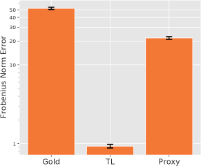
Figure 2 shows the Frobenius error of the our transfer learning estimator as well as the classical low-rank estimators on gold and proxy data alone. Details of synthetic data generation and setup are given in Appendix 13.1. As expected, our transfer learning estimator exploits the group-sparse bias term to significantly outperform the other two estimators—i.e., the Frobenius error of our transfer learning estimator is only around 4% of the proxy estimator and 2% of the gold estimator.

Refer to caption
Figure 2: Frobenius norm estimation error of $\Theta_{g}$ averaged over 100 trials, with 95% confidence intervals.

5.2 Wikipedia

A significant advantage of our method is that it is more interpretable—e.g., it can be used to identify domain-specific words (i.e., words that have a special meaning/usage in the target domain).

In this experiment, we evaluate our approach on 37 individual domain-specific Wikipedia articles from the following four domains: finance, math, computer science, and politics. The articles selected all have a domain-specific word in their title—e.g., “put” in the article “put option” (in finance), “closed” in “closed set” (in math), “object” in computing, and “left” in “left wing politics” (in politics). We define a word to be a domain word if any of its definitions on Wiktionary is labeled with key words from that domain—i.e., “finance” or “business” for finance, “math”, “geometry”, “algebra”, or “group theory” for math, “computing” or “programming” for computer science, and “politics” for politics.

We leverage our transfer learning approach on the GloVe objective and evaluate its performance at identifying domain-specific words on individual domain-specific Wikipedia articles. Details are provided in Appendix 13.2. We compare our approach with a state-of-the-art fine-tuning heuristic Mittens (Dingwall and Potts 2018), as well as random word selection. Table 5.1 shows the $F_{1}$-score of the selected domain words (weighted by article length) across articles in each domain. While we observe that other approaches also identify domain-specific words, our approach does so more effectively, most likely since our group-sparsity assumption is at least partly supported by these datasets. Table 5.2 shows the top 10 words ranked by our approach and by Mittens for one article in each domain; our approach is more effective at identifying domain-specific words (in bold).

\SingleSpacedXI
Domain TL Mittens Random
Finance 0.2280 0.1912 0.1379
Math 0.2546 0.2171 0.1544
Computing 0.2613 0.1952 0.1436
Politics 0.1852 0.1543 0.0634
Table 5.1: Weighted F1-score of domain word identification across four domains; we select the top 10% of words. “TL” represents our transfer learning approach.
\SingleSpacedXI
Short Prime Number Cloud Computing Conservatism
TL Mittens TL Mittens TL Mittens TL Mittens
short short prime prime cloud cloud party party
shares percent formula still data private conservative conservative
price due numbers formula computing large social second
stock public number de service information conservatism social
security customers primes numbers services devices government research
selling prices theorem number applications applications liberal svp
securities high natural great private security conservatives government
position hard integers side users work political de
may shares theory way use engine right also
margin price product algorithm software allows economic church
Table 5.2: Top 10 words in the rank sorted by absolute change of word embedding from source to target domain; domain words are labeled in bold. The threshold is set to top 10% of the rank.

5.3 Clinical Trial Eligibility

Another measure of the quality of word embeddings is the prediction accuracy in a downstream task that leverages these embeddings as features. To this end, we consider a clinical trial eligibility prediction task, where the words are from the medical domain.

The inclusion criteria for cancer clinical trials are restrictive, and these protocols are typically described in free-text clinical statements. In this experiment, we analyze a subsample of a clinical trial eligibility data used in Bustos and Pertusa (2018), which is publicly available on Kaggle.222https://www.kaggle.com/auriml/eligibilityforcancerclinicaltrials The data provides a label (eligible or not eligible), and a corresponding short free-text statement that describes the eligibility criterion and the study intervention and condition.

We apply our approach in conjunction with GloVe, and compare it with Mittens. To illustrate the generality of our approach, we also compare our method and Mittens over alternative pre-trained word embeddings (i.e., other than GloVe), including Word2Vec (Mikolov et al. 2013) and Dict2Vec (Tissier et al. 2017), which extends Word2Vec by adding dictionary definition of words.

To predict eligibility, we use regularized logistic regression with an $\ell_{2}$ penalty, chosen via 5-fold cross-validation. Table 5.3 shows the average $F_{1}$-score over 10,000 trials and 95% confidence intervals. Our transfer learning estimator outperforms all baselines on the downstream prediction task. Furthermore, the improved performance of our transfer learning estimator is robust across different pre-trained word embeddings.

\SingleSpacedXI
Pre-trained Estimator Average F1-score
GloVe TL $\textbf{0.612554}\pm 0.003405$
Mittens $0.604338\pm 0.003413$
Gold $0.583299\pm 0.003516$
Proxy $0.568205\pm 0.003465$
Word2Vec TL $\textbf{0.624428}\pm 0.003466$
Mittens $0.604981\pm 0.003514$
Proxy $0.580473\pm 0.003503$
Dict2Vec TL $\textbf{0.638923}\pm 0.003154$
Mittens $0.627772\pm 0.003335$
Proxy $0.623337\pm 0.003491$
Table 5.3: F1-score of prediction (averaged over 10,000 trials) with 95% confidence intervals.

6 Conclusions

We propose a novel estimator for transferring knowledge from large text corpora to learn word embeddings in a data-scarce domain of interest. We cast this as a low-rank matrix factorization problem with a group-sparse penalty, regularizing the domain embeddings towards existing pre-trained embeddings. Under a group-sparsity assumption and standard regularity conditions, we prove that our estimator requires substantially less data to achieve the same error compared to conventional estimators that do not leverage transfer learning. Our experiments demonstrate the effectiveness of our approach in the low-data regime on synthetic data, a domain word identification task on Wikipedia articles, and a downstream clinical trial eligibility prediction task.

While our focus has been on learning word embeddings, unsupervised matrix factorization models have also been widely applied for recommender systems and causal inference, which may open up new lines of inquiry. For instance, in recommender systems, one could consider a bandit approach that further collects domain-specific data in an online fashion (Kallus and Udell 2020); in causal inference, one could treat counterfactuals as missing data and leverage a factor model (Xiong and Pelger 2019). There has also been significant recent interest in low-rank tensor recovery problems (Goldfarb and Qin 2014, Zhang et al. 2019, Shah and Yu 2019), where one aims to learn to make recommendations across multiple types of outcomes (Farias and Li 2019) or to learn treatment effects across multiple experiments (Agarwal et al. 2020). Our transfer learning approach can be used in conjunction with these methods in order to leverage data from other domains.

\ACKNOWLEDGMENT

The authors gratefully acknowledge helpful feedback from various seminar participants, and indispensable financial support from the Wharton Analytics Initiative and the Wharton Dean’s Fund.

\SingleSpacedXI

References

  • Agarwal et al. (2012) Agarwal, Alekh, Sahand Negahban, Martin J Wainwright. 2012. Noisy matrix decomposition via convex relaxation: Optimal rates in high dimensions. The Annals of Statistics 1171–1197.
  • Agarwal et al. (2020) Agarwal, Anish, Devavrat Shah, Dennis Shen. 2020. Synthetic interventions. arXiv preprint arXiv:2006.07691 .
  • Ali et al. (2020) Ali, Alnur, Edgar Dobriban, Ryan Tibshirani. 2020. The implicit regularization of stochastic gradient flow for least squares. International Conference on Machine Learning. PMLR, 233–244.
  • Bastani (2020) Bastani, Hamsa. 2020. Predicting with proxies: Transfer learning in high dimension. Management Science .
  • Bellstam et al. (2020) Bellstam, Gustaf, Sanjai Bhagat, J Anthony Cookson. 2020. A text-based analysis of corporate innovation. Management Science .
  • Ben-David et al. (2010) Ben-David, Shai, John Blitzer, Koby Crammer, Alex Kulesza, Fernando Pereira, Jennifer Wortman Vaughan. 2010. A theory of learning from different domains. Machine learning 79(1) 151–175.
  • Ben-David et al. (2007) Ben-David, Shai, John Blitzer, Koby Crammer, Fernando Pereira, et al. 2007. Analysis of representations for domain adaptation. Advances in neural information processing systems 19 137.
  • Bhojanapalli et al. (2016) Bhojanapalli, Srinadh, Behnam Neyshabur, Nathan Srebro. 2016. Global optimality of local search for low rank matrix recovery. arXiv preprint arXiv:1605.07221 .
  • Blitzer et al. (2007) Blitzer, John, Mark Dredze, Fernando Pereira. 2007. Biographies, bollywood, boom-boxes and blenders: Domain adaptation for sentiment classification. Proceedings of the 45th annual meeting of the association of computational linguistics. 440–447.
  • Boucheron et al. (2013) Boucheron, Stéphane, Gábor Lugosi, Pascal Massart. 2013. Concentration inequalities: A nonasymptotic theory of independence. Oxford university press.
  • Burer and Monteiro (2003) Burer, Samuel, Renato DC Monteiro. 2003. A nonlinear programming algorithm for solving semidefinite programs via low-rank factorization. Mathematical Programming 95(2) 329–357.
  • Bustos and Pertusa (2018) Bustos, Aurelia, Antonio Pertusa. 2018. Learning eligibility in cancer clinical trials using deep neural networks. Applied Sciences 8(7) 1206.
  • Candes and Plan (2011) Candes, Emmanuel J, Yaniv Plan. 2011. Tight oracle inequalities for low-rank matrix recovery from a minimal number of noisy random measurements. IEEE Transactions on Information Theory 57(4) 2342–2359.
  • Chi et al. (2019) Chi, Yuejie, Yue M Lu, Yuxin Chen. 2019. Nonconvex optimization meets low-rank matrix factorization: An overview. IEEE Transactions on Signal Processing 67(20) 5239–5269.
  • Dingwall and Potts (2018) Dingwall, Nicholas, Christopher Potts. 2018. Mittens: an extension of glove for learning domain-specialized representations. Proceedings of the 2018 Conference of the North American Chapter of the Association for Computational Linguistics: Human Language Technologies, Volume 2 (Short Papers). 212–217.
  • Farias and Li (2019) Farias, Vivek F, Andrew A Li. 2019. Learning preferences with side information. Management Science 65(7) 3131–3149.
  • Friedman et al. (2010) Friedman, Jerome, Trevor Hastie, Robert Tibshirani. 2010. A note on the group lasso and a sparse group lasso. arXiv preprint arXiv:1001.0736 .
  • Ganin and Lempitsky (2015) Ganin, Yaroslav, Victor Lempitsky. 2015. Unsupervised domain adaptation by backpropagation. International conference on machine learning. PMLR, 1180–1189.
  • Ge et al. (2017) Ge, Rong, Chi Jin, Yi Zheng. 2017. No spurious local minima in nonconvex low rank problems: A unified geometric analysis. Proceedings of the 34th International Conference on Machine Learning-Volume 70. JMLR. org, 1233–1242.
  • Goldfarb and Qin (2014) Goldfarb, Donald, Zhiwei Qin. 2014. Robust low-rank tensor recovery: Models and algorithms. SIAM Journal on Matrix Analysis and Applications 35(1) 225–253.
  • Hsu et al. (2020) Hsu, Chao-Chun, Shantanu Karnwal, Sendhil Mullainathan, Ziad Obermeyer, Chenhao Tan. 2020. Characterizing the value of information in medical notes. Findings of the Association for Computational Linguistics: EMNLP 2020. Association for Computational Linguistics, Online, 2062–2072. 10.18653/v1/2020.findings-emnlp.187. URL https://www.aclweb.org/anthology/2020.findings-emnlp.187.
  • Hsu et al. (2012) Hsu, Daniel, Sham Kakade, Tong Zhang, et al. 2012. A tail inequality for quadratic forms of subgaussian random vectors. Electronic Communications in Probability 17.
  • Kallus and Udell (2020) Kallus, Nathan, Madeleine Udell. 2020. Dynamic assortment personalization in high dimensions. Operations Research 68(4) 1020–1037.
  • Levy and Goldberg (2014) Levy, Omer, Yoav Goldberg. 2014. Neural word embedding as implicit matrix factorization. Advances in neural information processing systems 27 2177–2185.
  • Li et al. (2019) Li, Qiuwei, Zhihui Zhu, Gongguo Tang. 2019. The non-convex geometry of low-rank matrix optimization. Information and Inference: A Journal of the IMA 8(1) 51–96.
  • Li et al. (2021) Li, Ruoting, Margaret Tobey, Maria Mayorga, Sherrie Caltagirone, Osman Özaltın. 2021. Detecting human trafficking: Automated classification of online customer reviews of massage businesses. Available at SSRN 3982796 .
  • Lipton et al. (2018) Lipton, Zachary, Yu-Xiang Wang, Alexander Smola. 2018. Detecting and correcting for label shift with black box predictors. International conference on machine learning. PMLR, 3122–3130.
  • Liu et al. (2016) Liu, Xiao, Param Vir Singh, Kannan Srinivasan. 2016. A structured analysis of unstructured big data by leveraging cloud computing. Marketing Science 35(3) 363–388.
  • Loh and Wainwright (2015) Loh, Po-Ling, Martin J Wainwright. 2015. Regularized m-estimators with nonconvexity: Statistical and algorithmic theory for local optima. The Journal of Machine Learning Research 16(1) 559–616.
  • Lounici et al. (2011) Lounici, Karim, Massimiliano Pontil, Sara Van De Geer, Alexandre B Tsybakov, et al. 2011. Oracle inequalities and optimal inference under group sparsity. The Annals of Statistics 39(4) 2164–2204.
  • Mankad et al. (2016) Mankad, Shawn, Hyunjeong “Spring” Han, Joel Goh, Srinagesh Gavirneni. 2016. Understanding online hotel reviews through automated text analysis. Service Science 8(2) 124–138.
  • Mikolov et al. (2013) Mikolov, Tomas, Ilya Sutskever, Kai Chen, Greg S Corrado, Jeff Dean. 2013. Distributed representations of words and phrases and their compositionality. Advances in neural information processing systems. 3111–3119.
  • Negahban and Wainwright (2011) Negahban, Sahand, Martin J Wainwright. 2011. Estimation of (near) low-rank matrices with noise and high-dimensional scaling. The Annals of Statistics 1069–1097.
  • Negahban and Wainwright (2012) Negahban, Sahand, Martin J Wainwright. 2012. Restricted strong convexity and weighted matrix completion: Optimal bounds with noise. The Journal of Machine Learning Research 13 1665–1697.
  • Negahban et al. (2012) Negahban, Sahand N, Pradeep Ravikumar, Martin J Wainwright, Bin Yu, et al. 2012. A unified framework for high-dimensional analysis of $m$-estimators with decomposable regularizers. Statistical science 27(4) 538–557.
  • Netzer et al. (2012) Netzer, Oded, Ronen Feldman, Jacob Goldenberg, Moshe Fresko. 2012. Mine your own business: Market-structure surveillance through text mining. Marketing Science 31(3) 521–543.
  • Ong et al. (2020) Ong, Charlene Jennifer, Agni Orfanoudaki, Rebecca Zhang, Francois Pierre M Caprasse, Meghan Hutch, Liang Ma, Darian Fard, Oluwafemi Balogun, Matthew I Miller, Margaret Minnig, et al. 2020. Machine learning and natural language processing methods to identify ischemic stroke, acuity and location from radiology reports. PloS one 15(6) e0234908.
  • Park et al. (2017) Park, Dohyung, Anastasios Kyrillidis, Constantine Carmanis, Sujay Sanghavi. 2017. Non-square matrix sensing without spurious local minima via the burer-monteiro approach. Artificial Intelligence and Statistics. PMLR, 65–74.
  • Pennington et al. (2014) Pennington, Jeffrey, Richard Socher, Christopher D Manning. 2014. Glove: Global vectors for word representation. Proceedings of the 2014 conference on empirical methods in natural language processing (EMNLP). 1532–1543.
  • Ramchandani et al. (2021) Ramchandani, Pia, Hamsa Bastani, Emily Wyatt. 2021. Unmasking human trafficking risk in commercial sex supply chains with machine learning. Available at SSRN 3866259 .
  • Raskutti et al. (2010) Raskutti, Garvesh, Martin J Wainwright, Bin Yu. 2010. Restricted eigenvalue properties for correlated gaussian designs. The Journal of Machine Learning Research 11 2241–2259.
  • Recht et al. (2007) Recht, Benjamin, Maryam Fazel, Pablo A Parrilo. 2007. Guaranteed minimum-rank solutions of linear matrix equations via nuclear norm minimization. arXiv preprint arXiv:0706.4138 .
  • Rigollet (2015) Rigollet, Philippe. 2015. 18. s997: High dimensional statistics. Lecture Notes, Cambridge, MA, USA: MIT Open-CourseWare .
  • Risch and Krestel (2019) Risch, Julian, Ralf Krestel. 2019. Domain-specific word embeddings for patent classification. Data Technologies and Applications .
  • Roy et al. (2017) Roy, Arpita, Youngja Park, SHimei Pan. 2017. Learning domain-specific word embeddings from sparse cybersecurity texts. arXiv preprint arXiv:1709.07470 .
  • Sarma et al. (2018) Sarma, Prathusha K, Yingyu Liang, William A Sethares. 2018. Domain adapted word embeddings for improved sentiment classification. arXiv preprint arXiv:1805.04576 .
  • Shah and Yu (2019) Shah, Devavrat, Christina Lee Yu. 2019. Iterative collaborative filtering for sparse noisy tensor estimation. 2019 IEEE International Symposium on Information Theory (ISIT). IEEE, 41–45.
  • Simon et al. (2013) Simon, Noah, Jerome Friedman, Trevor Hastie, Robert Tibshirani. 2013. A sparse-group lasso. Journal of computational and graphical statistics 22(2) 231–245.
  • Tissier et al. (2017) Tissier, Julien, Christophe Gravier, Amaury Habrard. 2017. Dict2vec: Learning word embeddings using lexical dictionaries. Proceedings of the 2017 Conference on Empirical Methods in Natural Language Processing. 254–263.
  • Xiong and Pelger (2019) Xiong, Ruoxuan, Markus Pelger. 2019. Large dimensional latent factor modeling with missing observations and applications to causal inference. arXiv preprint arXiv:1910.08273 .
  • Xu et al. (2021) Xu, Kan, Xuanyi Zhao, Hamsa Bastani, Osbert Bastani. 2021. Group-sparse matrix factorization for transfer learning of word embeddings. International Conference on Machine Learning. PMLR, 11603–11612.
  • Yang et al. (2017) Yang, Wei, Wei Lu, Vincent Zheng. 2017. A simple regularization-based algorithm for learning cross-domain word embeddings. Proceedings of the 2017 Conference on Empirical Methods in Natural Language Processing. 2898–2904.
  • Zhang et al. (2013) Zhang, Kun, Bernhard Schölkopf, Krikamol Muandet, Zhikun Wang. 2013. Domain adaptation under target and conditional shift. International Conference on Machine Learning. PMLR, 819–827.
  • Zhang et al. (2019) Zhang, Xiaoqin, Di Wang, Zhengyuan Zhou, Yi Ma. 2019. Robust low-rank tensor recovery with rectification and alignment. IEEE Transactions on Pattern Analysis and Machine Intelligence 43(1) 238–255.
{APPENDICES}

7 Quadratic Compatibility Condition

Proof 7.1

Proof of Proposition 2.7 The RSC condition gives

$\displaystyle\frac{1}{n}\|\mathcal{A}(\Delta U^{*T}+U^{*}\Delta^{T}+\Delta\Delta^{T})\|^{2}\geq\eta\|\Delta U^{*T}+U^{*}\Delta^{T}+\Delta\Delta^{T}\|_{F}^{2}-\tau(\sqrt{\frac{r}{n}}+\sqrt{\frac{\log d}{n}})^{2}\|\Delta\|_{2,1}^{2}.$ (13)

We lower bound the first term in inequality (13):

$\displaystyle\|\Delta U^{*T}+U^{*}\Delta^{T}+\Delta\Delta^{T}\|_{F}^{2}=$ $\displaystyle\|\Delta U^{*T}+U^{*}\Delta^{T}\|_{F}^{2}+\|\Delta\Delta^{T}\|_{F}^{2}+4\langle U^{*}\Delta^{T},\Delta\Delta^{T}\rangle$
$\displaystyle=$ $\displaystyle 4\|\Delta U^{*T}\|_{F}^{2}+\|\Delta\Delta^{T}\|_{F}^{2}+4\langle U^{*}\Delta^{T},\Delta\Delta^{T}\rangle$
$\displaystyle\geq$ $\displaystyle 4\|\Delta U^{*T}\|_{F}^{2}+\|\Delta\Delta^{T}\|_{F}^{2}-4|U^{*}\Delta^{T}|_{\infty}|\Delta\Delta^{T}|_{1}$
$\displaystyle\geq$ $\displaystyle 4\|\Delta U^{*T}\|_{F}^{2}+\|\Delta\Delta^{T}\|_{F}^{2}-4\|U^{*}\|_{2,\infty}\|\Delta\|_{2,\infty}\|\Delta\|_{2,1}^{2}$
$\displaystyle\geq$ $\displaystyle 4\|\Delta U^{*T}\|_{F}^{2}+\|\Delta\Delta^{T}\|_{F}^{2}-4\frac{D\bar{L}}{\sqrt{d}}\|\Delta\|_{2,1}^{2}.$

where the second equality uses $\operatorname{tr}(X^{2})=\|X\|_{F}^{2}$. This gives us

$$\frac{1}{n}\|\mathcal{A}(\Delta U^{*T}+U^{*}\Delta^{T}+\Delta\Delta^{T})\|^{2}\geq 4\eta\|\Delta U^{*T}\|_{F}^{2}+\eta\|\Delta\Delta^{T}\|_{F}^{2}\\ -4\frac{\eta D\bar{L}}{\sqrt{d}}\|\Delta\|_{2,1}^{2}-\tau(\sqrt{\frac{r}{n}}+\sqrt{\frac{\log d}{n}})^{2}\|\Delta\|_{2,1}^{2}.$$

Under the condition that

$\displaystyle\sum_{j\in J^{c}}\|\Delta^{j}\|\leq 7\sum_{j\in J}\|\Delta^{j}\|,$

we can upper bound $\|\Delta\|_{2,1}^{2}$ with a constant scale of $\|\Delta\|_{F}^{2}$:

$\displaystyle\|\Delta\|_{2,1}^{2}=(\sum_{j\in J^{c}}\|\Delta^{j}\|+\sum_{j\in J}\|\Delta^{j}\|)^{2}\leq(8\sum_{j\in J}\|\Delta^{j}\|)^{2}\leq 64s\|\Delta\|_{F}^{2}.$

Therefore, we have

$$\frac{1}{n}\|\mathcal{A}(\Delta U^{*T}+U^{*}\Delta^{T}+\Delta\Delta^{T})\|^{2}\geq\frac{4\eta\sigma_{r}(U^{*})^{2}}{s}(\sum_{j\in J}\|\Delta^{j}\|)^{2}+\eta\|\Delta\Delta^{T}\|_{F}^{2}\\ -64\left(4\frac{\eta D\bar{L}}{\sqrt{d}}+\tau(\sqrt{\frac{r}{n}}+\sqrt{\frac{\log d}{n}})^{2}\right)(\sum_{j\in J}\|\Delta^{j}\|)^{2}.$$

As long as $n$ and $d$ are such that

$\displaystyle\frac{\eta\sigma_{r}(U^{*})^{2}}{32s}\geq 4\frac{\eta D\bar{L}}{\sqrt{d}}+\tau(\sqrt{\frac{r}{n}}+\sqrt{\frac{\log d}{n}})^{2},$

we can derive the quadratic compatibility condition

$\displaystyle\frac{1}{n}\|\mathcal{A}(\Delta U^{*T}+U^{*}\Delta^{T}+\Delta\Delta^{T})\|^{2}\geq\frac{2\eta\sigma_{r}(U^{*})^{2}}{s}(\sum_{j\in J}\|\Delta^{j}\|)^{2}$

with $\kappa=2\eta\sigma_{r}(U^{*})^{2}$. \Halmos

Proof 7.2

Proof of Proposition 2.8 Our proof follows a similar strategy as Raskutti et al. (2010), Negahban and Wainwright (2011). Let $\bar{\mathcal{A}}:\mathbb{R}^{d\times d}\rightarrow\mathbb{R}^{n}$ with $\operatorname{vec}(\bar{A}_{g,i})\sim N(0,I)$. Then, we have by construction $\mathcal{A}(\Theta)=\bar{\mathcal{A}}(T_{\Sigma}(\Theta))$. In the following, we spare the use of the subscript $g$ to represent gold data whenever no confusions are caused.

Consider the set $\mathcal{R}(t)=\{\Delta\mid\|T_{\Sigma}(\Delta U^{*T}+U^{*}\Delta^{T}+\Delta\Delta^{T})\|_{F}=b,\|\Delta\|_{2,1}\leq t\}$ for any given $b>0$. We aim to lower bound

$$\inf_{\Delta\in\mathcal{R}(t)}\|\mathcal{A}(\Delta U^{*T}+U^{*}\Delta^{T}+\Delta\Delta^{T})\|=\inf_{\Delta\in\mathcal{R}(t)}\sup_{u\in S^{n-1}}\langle u,\mathcal{A}(\Delta U^{*T}+U^{*}\Delta^{T}+\Delta\Delta^{T})\rangle,$$

where $S^{n-1}$ is the $n-1$ dimensional unit sphere. We establish the lower bound using Gaussian comparison inequalities, specifically Gordon’s inequality (Raskutti et al. 2010). We define an associated zero-mean Gaussian random variable $Z_{u,\Delta}=\langle u,\bar{\mathcal{A}}(\frac{T_{\Sigma}(\Delta U^{*T}+U^{*}\Delta^{T}+\Delta\Delta^{T})}{b})\rangle$. For any pairs $(u,\Delta)$ and $(u^{\prime},\Delta^{\prime})$, we have

$\displaystyle\mathbb{E}[(Z_{u,\Delta}-Z_{u^{\prime},\Delta^{\prime}})^{2}]=\|u\otimes\frac{T_{\Sigma}(\Delta U^{*T}+U^{*}\Delta^{T}+\Delta\Delta^{T})}{b}-u^{\prime}\otimes\frac{T_{\Sigma}(\Delta^{\prime}U^{*T}+U^{*}\Delta^{\prime T}+\Delta^{\prime}\Delta^{\prime T})}{b}\|_{F}^{2},$

where $\otimes$ is the Kronecker product. Now consider a second zero-mean Gaussian process $Y_{u,\Delta}=\langle g,u\rangle+\langle G,\frac{T_{\Sigma}(\Delta U^{*T}+U^{*}\Delta^{T}+\Delta\Delta^{T})}{b}\rangle$, where $g\in\mathbb{R}^{n}$ and $G\in\mathbb{R}^{d\times d}$ have i.i.d. $N(0,1)$ entries. For any pairs $(u,\Delta)$ and $(u^{\prime},\Delta^{\prime})$, we have

$\displaystyle\mathbb{E}[(Y_{u,\Delta}-Y_{u^{\prime},\Delta^{\prime}})^{2}]=\|u-u^{\prime}\|^{2}+\|\frac{T_{\Sigma}(\Delta U^{*T}+U^{*}\Delta^{T}+\Delta\Delta^{T})}{b}-\frac{T_{\Sigma}(\Delta^{\prime}U^{*T}+U^{*}\Delta^{\prime T}+\Delta^{\prime}\Delta^{\prime T})}{b}\|_{F}^{2}.$

As $\|u\|=1$ and $\|\frac{T_{\Sigma}(\Delta U^{*T}+U^{*}\Delta^{T}+\Delta\Delta^{T})}{b}\|_{F}=1$, it holds that

$$\|u\otimes\frac{T_{\Sigma}(\Delta U^{*T}+U^{*}\Delta^{T}+\Delta\Delta^{T})}{b}-u^{\prime}\otimes\frac{T_{\Sigma}(\Delta^{\prime}U^{*T}+U^{*}\Delta^{\prime T}+\Delta^{\prime}\Delta^{\prime T})}{b}\|_{F}^{2}\\ \leq\|u-u^{\prime}\|^{2}+\|\frac{T_{\Sigma}(\Delta U^{*T}+U^{*}\Delta^{T}+\Delta\Delta^{T})}{b}-\frac{T_{\Sigma}(\Delta^{\prime}U^{*T}+U^{*}\Delta^{\prime T}+\Delta^{\prime}\Delta^{\prime T})}{b}\|_{F}^{2},$$

where we use the fact that for any matrix $X,X^{\prime}$ with $\|X\|_{F}=\|X^{\prime}\|_{F}$

$\displaystyle\langle X,X-X^{\prime}\rangle\geq 0.$

When $\Delta=\Delta^{\prime}$, equality holds. Consequently, Gordon’s inequality gives rise to

$\displaystyle\mathbb{E}\left[\inf_{\Delta\in\mathcal{R}(t)}\sup_{u\in S^{n-1}}Z_{u,\Delta}\right]\geq\mathbb{E}\left[\inf_{\Delta\in\mathcal{R}(t)}\sup_{u\in S^{n-1}}Y_{u,\Delta}\right].$

The Gaussian process $Y_{u,\Delta}$ has

$\displaystyle\mathbb{E}\left[\inf_{\Delta\in\mathcal{R}(t)}\sup_{u\in S^{n-1}}Y_{u,\Delta}\right]=$ $\displaystyle\mathbb{E}\left[\sup_{u\in S^{n-1}}\langle g,u\rangle\right]+\mathbb{E}\left[\inf_{\Delta\in\mathcal{R}(t)}\langle G,\frac{T_{\Sigma}(\Delta U^{*T}+U^{*}\Delta^{T}+\Delta\Delta^{T})}{b}\rangle\right]$
$\displaystyle=$ $\displaystyle\mathbb{E}\left[\|g\|\right]-\mathbb{E}\left[\sup_{\Delta\in\mathcal{R}(t)}\langle G,\frac{T_{\Sigma}(\Delta U^{*T}+U^{*}\Delta^{T}+\Delta\Delta^{T})}{b}\rangle\right].$

Using Lemma 12.13, we can get $\mathbb{E}\left[\|g\|\right]\geq\frac{\sqrt{n}}{2}$ by calculation. Now by definition of $\mathcal{R}(t)$,

$\displaystyle\langle G,\frac{T_{\Sigma}(\Delta U^{*T}+U^{*}\Delta^{T}+\Delta\Delta^{T})}{b}\rangle$ $\displaystyle=\frac{1}{b}\langle T_{\Sigma}(G),\Delta U^{*T}+U^{*}\Delta^{T}+\Delta\Delta^{T}\rangle$
$\displaystyle=\frac{1}{b}\langle T_{\Sigma}(G)U^{*},\Delta\rangle+\langle T_{\Sigma}(G)^{T}U^{*},\Delta\rangle+\langle T_{\Sigma}(G),\Delta\Delta^{T}\rangle$
$\displaystyle\leq\frac{1}{b}(\|T_{\Sigma}(G)U^{*}\|_{2,\infty}+\|T_{\Sigma}(G)^{T}U^{*}\|_{2,\infty}+\bar{L}|T_{\Sigma}(G)|_{\infty})\|\Delta\|_{2,1},$

where we use $\|\Delta\|_{2,1}\leq\bar{L}$. Note that $\operatorname{vec}(T_{\Sigma}(G))\sim N(0,\Sigma)$. Lemma 12.11 gives that

$\displaystyle\mathbb{E}[|T_{\Sigma}(G)|_{\infty}]\leq 2\sqrt{\max_{i\in[d^{2}]}\Sigma_{ii}\log(\sqrt{2}d)}.$

On the other hand, Lemma 12.9, 12.11 and 12.13 yields that

$\displaystyle\mathbb{E}[\|T_{\Sigma}(G)U^{*}\|_{2,\infty}]$ $\displaystyle\leq\max_{i\in[d]}\sqrt{\operatorname{tr}(U^{*T}\bar{\Sigma}_{ii}U^{*})}+\sqrt{2\max_{i\in[d]}\|U^{*T}\bar{\Sigma}_{ii}U^{*}\|\log d}$
$\displaystyle\leq\sigma_{1}(U^{*})\max_{i\in[d]}\sqrt{\sigma_{1}(\bar{\Sigma}_{ii})}(\sqrt{r}+\sqrt{2\log d}).$

Similar results hold for $\mathbb{E}[\|T_{\Sigma}(G)^{T}U^{*}\|_{2,\infty}]$. Define $\Sigma^{\prime}$ to be such that $\operatorname{vec}(T_{\Sigma}(G)^{T})\sim N(0,\Sigma^{\prime})$ and hence $\Sigma^{\prime}=K^{(d,d)}\Sigma K^{(d,d)}$. $K^{(d,d)}\in\mathbb{R}^{d^{2}\times d^{2}}$ is a commutation matrix that transform $\operatorname{vec}(X)$ to $\operatorname{vec}(X^{T})$ for $X\in\mathbb{R}^{d\times d}$:

$$K^{(d,d)}\operatorname{vec}(X)=\operatorname{vec}(X^{T}).$$

Note that $\Sigma^{\prime}$ shares a similar property as $\Sigma$ as $K^{(d,d)}$ is nonsingular and has only eigenvalues $1$ or $-1$. Therefore, we can obtain

$$\mathbb{E}[\|T_{\Sigma}(G)U^{*}\|_{2,\infty}+\|T_{\Sigma}(G)^{T}U^{*}\|_{2,\infty}+\bar{L}|T_{\Sigma}(G)|_{\infty}]\\ \leq C_{6}(\sqrt{\log(\sqrt{2}d)}+(\sqrt{r}+\sqrt{2\log d}))\leq C_{6}(2\sqrt{r}+3\sqrt{\log d}),$$

where

$\displaystyle C_{6}=2\bar{L}\sqrt{\max_{i\in[d^{2}]}\Sigma_{ii}}+\sigma_{1}(U^{*})(\max_{i\in[d]}\sqrt{\sigma_{1}(\bar{\Sigma}_{ii})}+\max_{i\in[d]}\sqrt{\sigma_{1}(\bar{\Sigma}^{\prime}_{ii})}).$

Combining all the above gives

$\displaystyle\mathbb{E}\left[\inf_{\Delta\in\mathcal{R}(t)}\|\bar{\mathcal{A}}(\frac{T_{\Sigma}(\Delta U^{*T}+U^{*}\Delta^{T}+\Delta\Delta^{T})}{b})\|\right]=\mathbb{E}\left[\inf_{\Delta\in\mathcal{R}(t)}\sup_{u\in S^{n-1}}Z_{u,\Delta}\right]\geq\frac{\sqrt{n}}{2}-\frac{C_{6}(2\sqrt{r}+3\sqrt{\log d})}{b}t.$

It’s easy to show that the function $f(\bar{\mathcal{A}}):=\inf_{\Delta\in\mathcal{R}(t)}\|\bar{\mathcal{A}}(\frac{T_{\Sigma}(\Delta U^{*T}+U^{*}\Delta^{T}+\Delta\Delta^{T})}{b})\|$ is $1$-Lipschitz.

Applying Lemma 12.7 then shows that

$\displaystyle\mathbb{P}\left(\sup_{\Delta\in\mathcal{R}(t)}(\frac{5}{8}-\frac{\|\mathcal{A}(\Delta U^{*T}+U^{*}\Delta^{T}+\Delta\Delta^{T})\|}{b\sqrt{n}})\geq\frac{3}{2}g(t)\right)\leq\exp(-\frac{ng(t)^{2}}{8}),$

where $g(t)=\frac{1}{8}+\frac{C_{6}(2\sqrt{r}+3\sqrt{\log d})t}{b\sqrt{n}}$. By a peeling argument from Section 4.4 of Raskutti et al. (2010), we can derive that

$\displaystyle\frac{\|\mathcal{A}(\Delta U^{*T}+U^{*}\Delta^{T}+\Delta\Delta^{T})\|}{b\sqrt{n}}\geq\frac{1}{4}-\frac{3C_{6}(2\sqrt{r}+3\sqrt{\log d})}{b\sqrt{n}}\|\Delta\|_{2,1}$

for any $\Delta\in\{\Delta\mid\|T_{\Sigma}(\Delta U^{*T}+U^{*}\Delta^{T}+\Delta\Delta^{T})\|_{F}=b\}$ holds with probability greater than $1-c\exp(-c^{\prime}n)$ for some positive constant $c,c^{\prime}$, which implies

$\displaystyle\frac{\|\mathcal{A}(\Delta U^{*T}+U^{*}\Delta^{T}+\Delta\Delta^{T})\|}{\sqrt{n}}\geq\frac{1}{4}\|T_{\Sigma}(\Delta U^{*T}+U^{*}\Delta^{T}+\Delta\Delta^{T})\|_{F}-\frac{3C_{6}(2\sqrt{r}+3\sqrt{\log d})}{\sqrt{n}}\|\Delta\|_{2,1}.\Halmos$

8 Error Bound of Transfer Learning Estimator

We first state a tail inequality that bound the estimation error of our transfer learning estimator with high probability.

Lemma 8.1

Assume $\mathcal{A}_{p}$ satisfies $2r$-RWC$(\alpha_{p},\beta_{p})$, and $\mathcal{A}_{g}$ satisfies the quadratic compatibility condition. Let $A_{g,i}^{lk}$ represent the $(l,k)$ entry of matrix $A_{g,i}$, $A_{g}^{lk}=\begin{bmatrix}A_{g,1}^{lk}&\cdots&A_{g,n_{g}}^{lk}\end{bmatrix}^{T}$. Define $\Psi_{j},\Phi_{j}\in\mathbb{R}^{r\times r}$ to be

$\displaystyle\Psi_{j}=U_{g}^{*T}\frac{A_{g}^{jT}A_{g}^{j}}{n_{g}}U_{g}^{*},\quad\Phi_{j}=U_{g}^{*T}\frac{(A_{g}^{Tj})^{T}A_{g}^{Tj}}{n_{g}}U_{g}^{*},$

where $A_{g}^{j},A_{g}^{Tj}\in\mathbb{R}^{n_{g}\times d}$ are matrices that stacks up the $j^{\text{th}}$ rows of $A_{g,i}$ and $A_{g,i}^{T},~{}i\in[n_{g}]$ respectively, i.e.,

$$A_{g}^{j}=\begin{bmatrix}A_{g,1}^{j}\\ A_{g,2}^{j}\\ \vdots\\ A_{g,n_{g}}^{j}\end{bmatrix},\quad A_{g}^{Tj}=\begin{bmatrix}A_{g,1}^{Tj}\\ A_{g,2}^{Tj}\\ \vdots\\ A_{g,n_{g}}^{Tj}\end{bmatrix}.$$

Then, our two-stage transfer learning estimator satisfies with any chosen values of $\lambda>0$ and $c>0$

$\displaystyle\|\widehat{U}_{g}-U_{g}^{*}\|_{2,1}\geq 16(\frac{\lambda s}{\kappa}+\frac{4\sqrt{d}c}{\sigma_{r}(U_{p}^{*})(3\alpha_{p}-2\beta_{p})})$

with probability at most

$\displaystyle 2(36\sqrt{2})^{2r(2d+1)}\exp(-\frac{L^{2}\sigma_{r}^{2}(U_{p}^{*})(3\alpha_{p}-2\beta_{p})^{2}n_{p}}{512\beta_{p}\sigma_{p}^{2}d})$
$\displaystyle+2d^{2}\exp\left(-\frac{\lambda^{2}n_{g}}{2048L^{2}\sigma_{g}^{2}(\max_{l,k}\|A_{g}^{lk}\|^{2}/n_{g})}\right)$
$\displaystyle+d\max_{j\in[d]}\exp\left(-(\sqrt{\frac{\frac{\lambda^{2}n_{g}}{256\sigma_{g}^{2}}-(\operatorname{tr}(\Psi_{j})-\frac{\|\Psi_{j}\|_{F}^{2}}{2\|\Psi_{j}\|})}{2\|\Psi_{j}\|}}-\frac{\|\Psi_{j}\|_{F}}{2\|\Psi_{j}\|})^{2}\right)$
$\displaystyle+d\max_{j\in[d]}\exp\left(-(\sqrt{\frac{\frac{\lambda^{2}n_{g}}{256\sigma_{g}^{2}}-(\operatorname{tr}(\Phi_{j})-\frac{\|\Phi_{j}\|_{F}^{2}}{2\|\Phi_{j}\|})}{2\|\Phi_{j}\|}}-\frac{\|\Phi_{j}\|_{F}}{2\|\Phi_{j}\|})^{2}\right)$
$\displaystyle+2(36\sqrt{2})^{2r(2d+1)}\exp(-\frac{c^{2}n_{p}}{8\beta_{p}\sigma_{p}^{2}}).$

The above concentration inequality shows that the estimation error of our transfer learning estimator consists of two parts, one regarding to the sparse recovery of $\Delta_{U}^{*}$ and one about the estimation error of $U_{p}^{*}$ in the first step.

Proof 8.2

Proof of Lemma 8.1

As problem (5) is equivalent to problem (3.1), we analyze problem (5) for simplicity.

Note that the row sparsity is immune to rotations, that is, for any orthogonal matrix $R$, $\Delta_{U}^{*}R$ is still row sparse. After our first step of finding the proxy estimator, we align $\widehat{U}_{p}$ with $U_{p}^{*}$ in the direction of $R_{(\widehat{U}_{p},U_{p}^{*})}$. By our definition,

$$U_{g}^{*}R_{(\widehat{U}_{p},U_{p}^{*})}=U_{p}^{*}R_{(\widehat{U}_{p},U_{p}^{*})}+\Delta_{U}^{*}R_{(\widehat{U}_{p},U_{p}^{*})}.$$

Through our previous analyses, $\widehat{U}_{p}$ is close to $U_{p}^{*}R_{(\widehat{U}_{p},U_{p}^{*})}$ with a high probability. Therefore, in our second step, we aim to find an estimator $\widehat{\Delta}_{U}$ for $\Delta_{U}^{*}R_{(\widehat{U}_{p},U_{p}^{*})}$ through $\ell_{2,1}$ penalty. For simplicity, we use $U_{g}^{*}$, $U_{p}^{*}$ and $\Delta_{U}^{*}$ to represent $U_{g}^{*}R_{(\widehat{U}_{p},U_{p}^{*})}$, $U_{p}^{*}R_{(\widehat{U}_{p},U_{p}^{*})}$ and $\Delta_{U}^{*}R_{(\widehat{U}_{p},U_{p}^{*})}$ respectively in the following analyses, which are aligned in the direction of $R_{(\widehat{U}_{p},U_{p}^{*})}$. Define the first-stage estimation error $\nu=\widehat{U}_{p}-U_{p}^{*}$ and $\widetilde{\Delta}_{U}=\Delta_{U}^{*}-\nu$. Thus, $U_{g}^{*}=U_{p}^{*}+\Delta_{U}^{*}=\widehat{U}_{p}+\widetilde{\Delta}_{U}$. Since $\widehat{U}_{p}$ carries the estimation error from the first step, the parameter we actually want to recover is $\widetilde{\Delta}_{U}$, which is approximately row sparse when the proxy data is huge. We define the adjoint of an operator $\mathcal{A}:\mathbb{R}^{d\times d}\rightarrow\mathbb{R}^{n}$ to be $\mathcal{A}^{*}:\mathbb{R}^{n}\rightarrow\mathbb{R}^{d\times d}$, with $\mathcal{A}^{*}(\epsilon)=\sum_{i=1}^{n}\epsilon_{i}A_{i}$.

As we search within $\|\Delta_{U}\|_{2,1}\leq 2L$ and $\|\Delta_{U}^{*}\|_{2,1}\leq L$, we require the following event to hold

$\displaystyle\mathcal{I}=\left\{\|\nu\|_{2,1}\leq L\right\}$ (14)

for $\widetilde{\Delta}_{U}$ to be feasible. Using a similar analysis to Theorem 4.1, we can show the event $\mathcal{I}$ takes place with a high probability

$$\mathbb{P}(\mathcal{I})\geq 1-2(36\sqrt{2})^{2r(2d+1)}\exp\left(-\frac{L^{2}\sigma_{r}^{2}(U_{p}^{*})(3\alpha_{p}-2\beta_{p})^{2}n_{p}}{512\beta\sigma_{p}^{2}d}\right)$$

on the event $\mathcal{I}$, the global optimality of $\widehat{\Delta}_{U}$ implies

$$\frac{1}{n_{g}}\|X_{g}-\mathcal{A}_{g}((\widehat{U}_{p}+\widehat{\Delta}_{U})(\widehat{U}_{p}+\widehat{\Delta}_{U})^{T})\|^{2}+\lambda\|\widehat{\Delta}_{U}\|_{2,1}\\ \leq\frac{1}{n_{g}}\|X_{g}-\mathcal{A}_{g}((\widehat{U}_{p}+\widetilde{\Delta}_{U})(\widehat{U}_{p}+\widetilde{\Delta}_{U})^{T})\|^{2}+\lambda\|\widetilde{\Delta}_{U}\|_{2,1}.$$

Plugging in $X_{g}=\mathcal{A}_{g}((\widehat{U}_{p}+\widetilde{\Delta}_{U})(\widehat{U}_{p}+\widetilde{\Delta}_{U})^{T})+\epsilon_{g}$ yields

$$\frac{1}{n_{g}}\|\mathcal{A}_{g}((\widehat{U}_{p}+\widehat{\Delta}_{U})(\widehat{U}_{p}+\widehat{\Delta}_{U})^{T}-(\widehat{U}_{p}+\widetilde{\Delta}_{U})(\widehat{U}_{p}+\widetilde{\Delta}_{U})^{T})\|^{2}+\lambda\|\widehat{\Delta}_{U}\|_{2,1}\\ \leq\frac{2}{n_{g}}\langle\epsilon_{g},\mathcal{A}_{g}((\widehat{U}_{p}+\widehat{\Delta}_{U})(\widehat{U}_{p}+\widehat{\Delta}_{U})^{T}-(\widehat{U}_{p}+\widetilde{\Delta}_{U})(\widehat{U}_{p}+\widetilde{\Delta}_{U})^{T})\rangle+\lambda\|\widetilde{\Delta}_{U}\|_{2,1}.$$

Rearranging the RHS with $U_{g}^{*}=\widehat{U}_{p}+\widetilde{\Delta}_{U}$, we get

$$\frac{1}{n_{g}}\|\mathcal{A}_{g}((\widehat{U}_{p}+\widehat{\Delta}_{U})(\widehat{U}_{p}+\widehat{\Delta}_{U})^{T}-(\widehat{U}_{p}+\widetilde{\Delta}_{U})(\widehat{U}_{p}+\widetilde{\Delta}_{U})^{T})\|^{2}+\lambda\|\widehat{\Delta}_{U}\|_{2,1}\\ \leq\frac{2}{n_{g}}\langle\epsilon_{g},\mathcal{A}_{g}((\widehat{\Delta}_{U}-\widetilde{\Delta}_{U})U_{g}^{*T}+U_{g}^{*}(\widehat{\Delta}_{U}-\widetilde{\Delta}_{U})^{T}+(\widehat{\Delta}_{U}-\widetilde{\Delta}_{U})(\widehat{\Delta}_{U}-\widetilde{\Delta}_{U})^{T})\rangle+\lambda\|\widetilde{\Delta}_{U}\|_{2,1}$$ (15)

The first part of the first term on the RHS of inequality (15) has

$\displaystyle\langle\epsilon_{g},\mathcal{A}_{g}((\widehat{\Delta}_{U}-\widetilde{\Delta}_{U})U_{g}^{*T}+U_{g}^{*}(\widehat{\Delta}_{U}-\widetilde{\Delta}_{U})^{T})\rangle=$ $\displaystyle\langle\mathcal{A}_{g}^{*}(\epsilon_{g}),(\widehat{\Delta}_{U}-\widetilde{\Delta}_{U})U_{g}^{*T}+U_{g}^{*}(\widehat{\Delta}_{U}-\widetilde{\Delta}_{U})^{T}\rangle$
$\displaystyle=$ $\displaystyle\langle\mathcal{A}_{g}^{*}(\epsilon_{g})U_{g}^{*},\widehat{\Delta}_{U}-\widetilde{\Delta}_{U}\rangle+\langle\mathcal{A}_{g}^{*}(\epsilon_{g})^{T}U_{g}^{*},\widehat{\Delta}_{U}-\widetilde{\Delta}_{U}\rangle$
$\displaystyle\leq$ $\displaystyle(\max_{j\in[d]}\|(\mathcal{A}_{g}^{*}(\epsilon_{g})^{j}U_{g}^{*}\|+\max_{j\in[d]}\|\mathcal{A}_{g}^{*}(\epsilon_{g})^{Tj}U_{g}^{*}\|)\|\widehat{\Delta}_{U}-\widetilde{\Delta}_{U}\|_{2,1}.$

Correspondingly, the second part of the first term on the RHS of inequality (15) has

$\displaystyle\langle\epsilon_{g},\mathcal{A}_{g}((\widehat{\Delta}_{U}-\widetilde{\Delta}_{U})(\widehat{\Delta}_{U}-\widetilde{\Delta}_{U})^{T})\rangle=$ $\displaystyle\langle\mathcal{A}_{g}^{*}(\epsilon_{g}),(\widehat{\Delta}_{U}-\widetilde{\Delta}_{U})(\widehat{\Delta}_{U}-\widetilde{\Delta}_{U})^{T}\rangle$
$\displaystyle\leq$ $\displaystyle|\mathcal{A}_{g}^{*}(\epsilon_{g})|_{\infty}|(\widehat{\Delta}_{U}-\widetilde{\Delta}_{U})(\widehat{\Delta}_{U}-\widetilde{\Delta}_{U})^{T}|_{1}$
$\displaystyle\leq$ $\displaystyle|\mathcal{A}_{g}^{*}(\epsilon_{g})|_{\infty}\|\widehat{\Delta}_{U}-\widetilde{\Delta}_{U}\|_{2,1}^{2}.$ (16)

Next, consider the following events

$$\mathcal{G}_{1}=\left\{\frac{2}{n_{g}}\max_{j\in[d]}\|\mathcal{A}_{g}^{*}(\epsilon_{g})^{j}U_{g}^{*}\|\leq\frac{\lambda}{8}\right\},\quad\mathcal{G}_{2}=\left\{\frac{2}{n_{g}}\max_{j\in[d]}\|\mathcal{A}_{g}^{*}(\epsilon_{g})^{Tj}U_{g}^{*}\|\leq\frac{\lambda}{8}\right\},$$

and

$$\mathcal{F}=\left\{\frac{2}{n_{g}}|\mathcal{A}_{g}^{*}(\epsilon_{g})|_{\infty}\leq\frac{\lambda}{16L}\right\},$$

which we prove holds with high probability in Lemma 8.3 after this lemma. On the events $\mathcal{G}_{1}$, $\mathcal{G}_{2}$ and $\mathcal{F}$, we derive from inequality (15) that

$$\frac{1}{n_{g}}\|\mathcal{A}_{g}((\widehat{U}_{p}+\widehat{\Delta}_{U})(\widehat{U}_{p}+\widehat{\Delta}_{U})^{T}-(\widehat{U}_{p}+\widetilde{\Delta}_{U})(\widehat{U}_{p}+\widetilde{\Delta}_{U})^{T})\|^{2}+\lambda\|\widehat{\Delta}_{U}\|_{2,1}\\ \leq\frac{\lambda}{4}\|\widehat{\Delta}_{U}-\widetilde{\Delta}_{U}\|_{2,1}+\frac{\lambda}{16L}\|\widehat{\Delta}_{U}-\widetilde{\Delta}_{U}\|_{2,1}^{2}+\lambda\|\widetilde{\Delta}_{U}\|_{2,1}\\ \leq\frac{\lambda}{2}\|\widehat{\Delta}_{U}-\widetilde{\Delta}_{U}\|_{2,1}+\lambda\|\widetilde{\Delta}_{U}\|_{2,1}.$$

The second inequality uses

$\displaystyle\|\widehat{\Delta}_{U}-\widetilde{\Delta}_{U}\|_{2,1}\leq 4L,$

which is derived from the definition of the search region $\|\Delta_{U}\|_{2,1}\leq 2L$, the definition of event $\mathcal{I}$, and the feasibility of $\Delta_{U}^{*}$ that $\|\Delta_{U}^{*}\|_{2,1}\leq L$. We can further arrange the inequality to get

$$\frac{1}{n_{g}}\|\mathcal{A}_{g}((\widehat{U}_{p}+\widehat{\Delta}_{U})(\widehat{U}_{p}+\widehat{\Delta}_{U})^{T}-(\widehat{U}_{p}+\widetilde{\Delta}_{U})(\widehat{U}_{p}+\widetilde{\Delta}_{U})^{T})\|^{2}+\frac{\lambda}{2}\sum_{j\in J^{c}}\|(\widehat{\Delta}_{U}-\widetilde{\Delta}_{U})^{j}\|\\ \leq\frac{3\lambda}{2}\sum_{j\in J}\|(\widehat{\Delta}_{U}-\widetilde{\Delta}_{U})^{j}\|+2\lambda\sum_{j\in J^{c}}\|\nu^{j}\|.$$ (17)

Now consider the following two cases respectively:

  1. (i).

    $\sum_{j\in J^{c}}\|\nu^{j}\|\leq\sum_{j\in J}\|(\widehat{\Delta}_{U}-\widetilde{\Delta}_{U})^{j}\|$,

  2. (ii).

    $\sum_{j\in J^{c}}\|\nu^{j}\|>\sum_{j\in J}\|(\widehat{\Delta}_{U}-\widetilde{\Delta}_{U})^{j}\|$.

Under Case (i), we derive from the inequality (17) that

$$\frac{1}{n_{g}}\|\mathcal{A}_{g}((\widehat{U}_{p}+\widehat{\Delta}_{U})(\widehat{U}_{p}+\widehat{\Delta}_{U})^{T}-(\widehat{U}_{p}+\widetilde{\Delta}_{U})(\widehat{U}_{p}+\widetilde{\Delta}_{U})^{T})\|^{2}+\frac{\lambda}{2}\sum_{j\in J^{c}}\|(\widehat{\Delta}_{U}-\widetilde{\Delta}_{U})^{j}\|\\ \leq\frac{7\lambda}{2}\sum_{j\in J}\|(\widehat{\Delta}_{U}-\widetilde{\Delta}_{U})^{j}\|.$$

Thus, we have $\sum_{j\in J^{c}}\|(\widehat{\Delta}_{U}-\widetilde{\Delta}_{U})^{j}\|\leq 7\sum_{j\in J}\|(\widehat{\Delta}_{U}-\widetilde{\Delta}_{U})^{j}\|$ and $\mathcal{A}_{g}$ satisfies the quadratic compatibility condition. Further write the above as

$$\frac{1}{n_{g}}\|\mathcal{A}_{g}((\widehat{U}_{p}+\widehat{\Delta}_{U})(\widehat{U}_{p}+\widehat{\Delta}_{U})^{T}-(\widehat{U}_{p}+\widetilde{\Delta}_{U})(\widehat{U}_{p}+\widetilde{\Delta}_{U})^{T})\|^{2}+\frac{\lambda}{2}\|\widehat{\Delta}_{U}-\widetilde{\Delta}_{U}\|_{2,1}\\ \leq\frac{8\lambda^{2}s}{\kappa}+\frac{\kappa}{2s}(\sum_{j\in J}\|(\widehat{\Delta}_{U}-\widetilde{\Delta}_{U})^{j}\|)^{2},$$

where we use the inequality $2ab\leq a^{2}+b^{2}$. Apply the quadratic compatibility condition to the RHS, and

$\displaystyle\frac{1}{2n_{g}}\|\mathcal{A}_{g}((\widehat{U}_{p}+\widehat{\Delta}_{U})(\widehat{U}_{p}+\widehat{\Delta}_{U})^{T}-(\widehat{U}_{p}+\widetilde{\Delta}_{U})(\widehat{U}_{p}+\widetilde{\Delta}_{U})^{T})\|^{2}+\frac{\lambda}{2}\|\widehat{\Delta}_{U}-\widetilde{\Delta}_{U}\|_{2,1}\leq\frac{8\lambda^{2}s}{\kappa}$

Under Case (ii), the inequality (17) gives

$$\frac{1}{n_{g}}\|\mathcal{A}((\widehat{U}_{p}+\widehat{\Delta}_{U})(\widehat{U}_{p}+\widehat{\Delta}_{U})^{T}-(\widehat{U}_{p}+\widetilde{\Delta}_{U})(\widehat{U}_{p}+\widetilde{\Delta}_{U})^{T})\|^{2}+\frac{\lambda}{2}\|\widehat{\Delta}_{U}-\widetilde{\Delta}_{U}\|_{2,1}\leq 4\lambda\sum_{j\in J^{c}}\|\nu^{j}\|.$$

Therefore, under any circumstances, we have

$$\|\widehat{\Delta}_{U}-\widetilde{\Delta}_{U}\|_{2,1}\leq 8(\frac{2\lambda s}{\kappa}+\sum_{j\in J^{c}}\|\nu^{j}\|)\leq 8(\frac{2\lambda s}{\kappa}+\|\nu\|_{2,1}).$$

Consider the event

$\displaystyle\mathcal{J}=\left\{\|\nu\|_{2,1}\leq\frac{8\sqrt{d}c}{(3\alpha_{p}-2\beta_{p})\sigma_{r}(U_{p}^{*})}\right\}.$ (18)

Using a similar analysis to Theorem 4.1 as our analysis on event $\mathcal{I}$, we have

$$\mathbb{P}(\mathcal{J})\geq 1-2(36\sqrt{2})^{2r(2d+1)}\exp(-\frac{c^{2}n_{p}}{8\beta_{p}\sigma_{p}^{2}}).$$

Therefore, on the event $\mathcal{J}$, the estimation error is bounded by

$$\|\widehat{\Delta}_{U}-\widetilde{\Delta}_{U}\|_{2,1}\leq 16(\frac{\lambda s}{\kappa}+\frac{4\sqrt{d}c}{(3\alpha_{p}-2\beta_{p})\sigma_{r}(U_{p}^{*})}).$$

Combining all the above and using Lemma 8.3, we have the following concentration inequality

$$\mathbb{P}\left(\|\widehat{\Delta}_{U}-\widetilde{\Delta}_{U}\|_{2,1}\geq 16(\frac{\lambda s}{\kappa}+\frac{4\sqrt{d}c}{(3\alpha_{p}-2\beta_{p})\sigma_{r}(U_{p}^{*})})\right)\\ \leq\mathbb{P}(\mathcal{I}^{c})+\mathbb{P}(\mathcal{G}_{1}^{c})+\mathbb{P}(\mathcal{G}_{2}^{c})+\mathbb{P}(\mathcal{F}^{c})+\mathbb{P}(\mathcal{J}^{c})\\ \leq 2(36\sqrt{2})^{2r(2d+1)}\exp(-\frac{L^{2}\sigma_{r}^{2}(U_{p}^{*})(3\alpha_{p}-2\beta_{p})^{2}n_{p}}{512\beta_{p}\sigma_{p}^{2}d})\\ +2d^{2}\exp\left(-\frac{\lambda^{2}n_{g}}{2048L^{2}\sigma_{g}^{2}(\max_{l,k}\|A_{g}^{lk}\|^{2}/n_{g})}\right)\\ +d\max_{j\in[d]}\exp\left(-(\sqrt{\frac{\frac{\lambda^{2}n_{g}}{256\sigma_{g}^{2}}-(\operatorname{tr}(\Psi_{j})-\frac{\|\Psi_{j}\|_{F}^{2}}{2\|\Psi_{j}\|})}{2\|\Psi_{j}\|}}-\frac{\|\Psi_{j}\|_{F}}{2\|\Psi_{j}\|})^{2}\right)\\ +d\max_{j\in[d]}\exp\left(-(\sqrt{\frac{\frac{\lambda^{2}n_{g}}{256\sigma_{g}^{2}}-(\operatorname{tr}(\Phi_{j})-\frac{\|\Phi_{j}\|_{F}^{2}}{2\|\Phi_{j}\|})}{2\|\Phi_{j}\|}}-\frac{\|\Phi_{j}\|_{F}}{2\|\Phi_{j}\|})^{2}\right)\\ +2(36\sqrt{2})^{2r(2d+1)}\exp(-\frac{c^{2}n_{p}}{8\beta_{p}\sigma_{p}^{2}}).\Halmos$$ (19)
Lemma 8.3

The events $\mathcal{G}_{1}$, $\mathcal{G}_{2}$ and $\mathcal{F}$ satisfy the following concentration inequalities

$\displaystyle\mathbb{P}(\mathcal{G}_{1}^{c})\leq d\max_{j\in[d]}\exp\left(-(\sqrt{\frac{\frac{\lambda^{2}n_{g}}{256\sigma_{g}^{2}}-(\operatorname{tr}(\Psi_{j})-\frac{\|\Psi_{j}\|_{F}^{2}}{2\|\Psi_{j}\|})}{2\|\Psi_{j}\|}}-\frac{\|\Psi_{j}\|_{F}}{2\|\Psi_{j}\|})^{2}\right),$
$\displaystyle\mathbb{P}(\mathcal{G}_{2}^{c})\leq d\max_{j\in[d]}\exp\left(-(\sqrt{\frac{\frac{\lambda^{2}n_{g}^{2}}{256\sigma_{g}^{2}}-(\operatorname{tr}(\Phi_{j})-\frac{\|\Phi_{j}\|_{F}^{2}}{2\|\Phi_{j}\|})}{2\|\Phi_{j}\|}}-\frac{\|\Phi_{j}\|_{F}}{2\|\Phi_{j}\|})^{2}\right),$

and

$\displaystyle\mathbb{P}(\mathcal{F}^{c})\leq 2d^{2}\exp\left(-\frac{\lambda^{2}n_{g}}{2048L^{2}\sigma_{g}^{2}(\max_{l,k}\|A_{g}^{lk}\|^{2}/n_{g})}\right).$
Proof 8.4

Proof of Lemma 8.3 Consider the event $\mathcal{F}$ first. With $\epsilon_{g}$ being $\sigma_{g}$-subgaussian,

$\displaystyle\mathbb{P}(\mathcal{F}^{c})$ $\displaystyle=\mathbb{P}(\frac{2}{n_{g}}|\mathcal{A}_{g}^{*}(\epsilon_{g})|_{\infty}\geq\frac{\lambda}{16L})$
$\displaystyle\leq d^{2}\max_{l,k\in[d]}\mathbb{P}(\frac{2}{n_{g}}|\sum_{i=1}^{n_{g}}A_{g,i}^{lk}\epsilon_{g,i}|\geq\frac{\lambda}{16L})$
$\displaystyle\leq 2d^{2}\exp\left(-\frac{\lambda^{2}n_{g}}{2048L^{2}\sigma_{g}^{2}(\max_{l,k}\|A_{g}^{lk}\|^{2}/n_{g})}\right),$

In the last inequality, we use the fact that $\epsilon_{g}$ is $\sigma_{g}$-subgaussian in the final inequality.

Next, we look at the event $\mathcal{G}_{1}$.

$\displaystyle\mathbb{P}(\mathcal{G}_{1}^{c})$ $\displaystyle=\mathbb{P}(\frac{2}{n_{g}}\max_{j\in[d]}\|\mathcal{A}_{g}^{*}(\epsilon_{g})^{j}U_{g}^{*}\|\geq\frac{\lambda}{8})$
$\displaystyle\leq d\max_{j\in[d]}\mathbb{P}(\frac{2}{n_{g}}\|\mathcal{A}_{g}^{*}(\epsilon_{g})^{j}U_{g}^{*}\|\geq\frac{\lambda}{8}).$

For a given $j$, observe that

$\displaystyle\frac{4}{n_{g}^{2}}\|\mathcal{A}_{g}^{*}(\epsilon_{g})^{j}U_{g}^{*}\|^{2}=\frac{4}{n_{g}^{2}}\|\sum_{i=1}^{n_{g}}A_{g,i}^{j}U_{g}^{*}\epsilon_{g,i}\|^{2}=\frac{4}{n_{g}}\epsilon_{g}^{T}\frac{A_{g}^{j}U_{g}^{*}U_{g}^{*T}A_{g}^{jT}}{n_{g}}\epsilon_{g},$

Note that $\Psi_{j}$ has the same positive eigenvalues as $\frac{A_{g}^{j}U_{g}^{*}U_{g}^{*T}A_{g}^{jT}}{n_{g}}$. Different from Lounici et al. (2011), we assume subgaussian random noises instead of Gaussian noises. Therefore, instead, we have from Lemma 12.5

$$\mathbb{P}(\frac{4}{n_{g}}\epsilon_{g}^{T}\frac{A_{g}^{j}U_{g}^{*}U_{g}^{*T}A_{g}^{jT}}{n_{g}}\epsilon_{g}\geq\frac{\lambda^{2}}{64})\leq\exp\left(-(\sqrt{\frac{\frac{\lambda^{2}n_{g}}{256\sigma_{g}^{2}}-(\operatorname{tr}(\Psi_{j})-\frac{\|\Psi_{j}\|_{F}^{2}}{2\|\Psi_{j}\|})}{2\|\Psi_{j}\|}}-\frac{\|\Psi_{j}\|_{F}}{2\|\Psi_{j}\|})^{2}\right).$$

Combining the results above, we can derive that

$\displaystyle\mathbb{P}(\mathcal{G}_{1}^{c})\leq d\max_{j\in[d]}\exp\left(-(\sqrt{\frac{\frac{\lambda^{2}n_{g}}{256\sigma_{g}^{2}}-(\operatorname{tr}(\Psi_{j})-\frac{\|\Psi_{j}\|_{F}^{2}}{2\|\Psi_{j}\|})}{2\|\Psi_{j}\|}}-\frac{\|\Psi_{j}\|_{F}}{2\|\Psi_{j}\|})^{2}\right).$

Similarly for event $\mathcal{G}_{2}$, we have

$\displaystyle\mathbb{P}(\mathcal{G}_{2}^{c})\leq d\max_{j\in[d]}\exp\left(-(\sqrt{\frac{\frac{\lambda^{2}n_{g}^{2}}{256\sigma_{g}^{2}}-(\operatorname{tr}(\Phi_{j})-\frac{\|\Phi_{j}\|_{F}^{2}}{2\|\Phi_{j}\|})}{2\|\Phi_{j}\|}}-\frac{\|\Phi_{j}\|_{F}}{2\|\Phi_{j}\|})^{2}\right).\Halmos$
Proof 8.5

Proof of Theorem 3.3 Theorem 3.3 follows Lemma 8.1. Suppose $\frac{L\sigma_{r}(U_{p}^{*})(3\alpha_{p}-2\beta_{p})}{8\sqrt{d}}\geq c$. On this event, the first term on the RHS of inequality (19) is smaller than the last term on the RHS. In order to make each term on the RHS to be smaller than $\frac{\delta}{5}$, we require

$\displaystyle\lambda\geq\max$ $\displaystyle\left\{\sqrt{\frac{2048L^{2}\sigma_{g}^{2}(\max_{l,k}\|A_{g}^{lk}\|^{2}/n_{g})}{n_{g}}\log(\frac{10d^{2}}{\delta})},\right.$
$\displaystyle\left.\max_{j\in[d]}\sqrt{\frac{256\sigma_{g}^{2}}{n_{g}}(\operatorname{tr}(\Psi_{j})+2\|\Psi_{j}\|_{F}\sqrt{\log(\frac{5d}{\delta})}+2\|\Psi_{j}\|\log(\frac{5d}{\delta}))},\right.$
$\displaystyle\left.\max_{j\in[d]}\sqrt{\frac{256\sigma_{g}^{2}}{n_{g}}(\operatorname{tr}(\Phi_{j})+2\|\Phi_{j}\|_{F}\sqrt{\log(\frac{5d}{\delta})}+2\|\Phi_{j}\|\log(\frac{5d}{\delta}))}\right\},$

and let $c$ take the value

$\displaystyle c=\sqrt{\frac{8\beta_{p}\sigma_{p}^{2}}{n_{p}}(2r(2d+1)\log(36\sqrt{2})+\log(\frac{10}{\delta}))}.$

Note that by definition of $1$-smoothness$(\beta_{g})$

$\displaystyle\frac{1}{n_{g}}\|A_{g}^{lk}\|^{2}=\langle E_{lk},\frac{1}{n_{g}}\mathcal{A}_{g}^{*}(\mathcal{A}_{g}(E_{lk}))\rangle\leq\beta_{g},$

where $E_{lk}\in\mathbb{R}^{d\times d}$ is a basis matrix whose $(l,k)$ entry is 1 and otherwise 0. On the other hand,

$\displaystyle\|\Psi_{j}\|$ $\displaystyle=\max_{\|x\|=1,x\in\mathbb{R}^{r}}x^{T}U_{g}^{*T}\frac{A_{g}^{jT}A_{g}^{j}}{n_{g}}U_{g}^{*}x$
$\displaystyle=\max_{\|x\|=1}x^{T}U_{g}^{*T}\frac{A_{g}^{jT}A_{g}^{j}}{n_{g}}U_{g}^{*}x.$

If we define a matrix $E_{j}(x)$ whose $j^{\text{th}}$ row is $x^{T}$ and otherwise 0, then

$\displaystyle\|\Psi_{j}\|$ $\displaystyle=\max_{\|x\|=1}\frac{1}{n_{g}}\langle E_{j}(U_{g}^{*}x),A_{g}^{*}(A_{g}(E_{j}(U_{g}^{*}x)))\rangle.$

As $\|x\|=1$, we have

$$\|E_{j}(U_{g}^{*}x)\|_{F}=\|U_{g}^{*}x\|\leq\sigma_{1}(U_{g}^{*}).$$

Therefore, we have

$\displaystyle\|\Psi_{j}\|$ $\displaystyle\leq\max_{\|R\|_{F}\leq\sigma_{1}(U_{g}^{*})}\frac{1}{n_{g}}\langle R,A_{g}^{*}(A_{g}(R)\rangle$
$\displaystyle\leq\beta_{g}\sigma_{1}^{2}(U_{g}^{*}).$

With a similar analysis, we have

$\displaystyle\|\Phi_{j}\|$ $\displaystyle\leq\beta_{g}\sigma_{1}^{2}(U_{g}^{*}).$

Given the above results, we can bound the trace and Frobenius norm of $\Psi_{j}$ and $\Phi_{j}$ proportional to their rank:

$\displaystyle\operatorname{tr}(\Psi_{j})\leq r\|\Psi_{j}\|\leq r\beta_{g}\sigma_{1}^{2}(U_{g}^{*}),\quad\|\Psi_{j}\|_{F}\leq\sqrt{r}\|\Psi_{j}\|\leq\sqrt{r}\beta_{g}\sigma_{1}^{2}(U_{g}^{*})$
$\displaystyle\operatorname{tr}(\Phi_{j})\leq r\beta_{g}\sigma_{1}^{2}(U_{g}^{*}),\quad\|\Phi_{j}\|_{F}\leq\sqrt{r}\beta_{g}\sigma_{1}^{2}(U_{g}^{*}).$

Combining all the above results, we can instead set $\lambda$ as:

$\displaystyle\lambda=\max$ $\displaystyle\left\{\sqrt{\frac{2048L^{2}\beta_{g}\sigma_{g}^{2}}{n_{g}}\log(\frac{10d^{2}}{\delta})},\right.$
$\displaystyle\left.\sqrt{\frac{256\beta_{g}\sigma_{g}^{2}\sigma_{1}^{2}(U_{g}^{*})}{n_{g}}(r+2\sqrt{r\log(\frac{5d}{\delta})}+2\log(\frac{5d}{\delta}))}\right\}.$

Therefore, with the above choice of $\lambda$ and with $n_{p}$ and $d$ such that

$$\sqrt{\frac{8\beta_{p}\sigma_{p}^{2}}{n_{p}}(2r(2d+1)\log(36\sqrt{2})+\log(\frac{10}{\delta}))}\leq\frac{L\sigma_{r}(U_{p}^{*})(3\alpha_{p}-2\beta_{p})}{8\sqrt{d}},$$

we obtain the following bound for estimation error of $\widetilde{\Delta}_{U}$:

$$\|\widehat{\Delta}_{U}-\widetilde{\Delta}_{U}\|_{2,1}=\mathcal{O}\left(\sqrt{\frac{\sigma_{g}^{2}s^{2}\log(\frac{d^{2}}{\delta})}{n_{g}}}+\sqrt{\frac{\sigma_{p}^{2}(d^{2}+d\log(\frac{1}{\delta}))}{n_{p}}}\right),$$

with probability greater than $1-\delta$. Consequently,

$$\ell(\widehat{U}_{g},U_{g}^{*})=\mathcal{O}\left(\sqrt{\frac{\sigma_{g}^{2}s^{2}\log(\frac{d^{2}}{\delta})}{n_{g}}}+\sqrt{\frac{\sigma_{p}^{2}(d^{2}+d\log(\frac{1}{\delta}))}{n_{p}}}\right),$$

with probability at least $1-\delta$. \Halmos

9 Local Minima

Proof 9.1

Proof of Proposition 3.4 By definition,

$\displaystyle\mathbb{E}_{X_{g}\mid\mathcal{A}_{g}}[\langle\nabla f(\widetilde{\Delta}_{U}+\Delta)-\nabla f(\widetilde{\Delta}_{U}),\Delta\rangle]=\frac{2}{n_{g}}\mathcal{A}_{g}(\Delta U_{g}^{*T}+U_{g}^{*}\Delta^{T}+\Delta\Delta^{T})^{T}\mathcal{A}_{g}(\Delta U_{g}^{*T}+U_{g}^{*}\Delta^{T}+2\Delta\Delta^{T}).$

As $\mathcal{A}_{g}$ satisfies RSC$(\sqrt{\frac{2}{3}}U_{g}^{*},\eta,\tau)$,

$\displaystyle\frac{2}{n_{g}}\mathcal{A}_{g}(\Delta U_{g}^{*T}+U_{g}^{*}\Delta^{T}+\Delta\Delta^{T})^{T}\mathcal{A}_{g}(\Delta U_{g}^{*T}+U_{g}^{*}\Delta^{T}+2\Delta\Delta^{T})$
$\displaystyle=$ $\displaystyle\frac{2}{n_{g}}(\|\mathcal{A}_{g}(\Delta U_{g}^{*T}+U_{g}^{*}\Delta^{T}+\frac{3}{2}\Delta\Delta^{T})\|^{2}-\frac{1}{4}\|\mathcal{A}_{g}(\Delta\Delta^{T})\|^{2})$
$\displaystyle\geq$ $\displaystyle 2\eta\|\Delta U_{g}^{*T}+U_{g}^{*}\Delta^{T}+\frac{3}{2}\Delta\Delta^{T}\|_{F}^{2}-\frac{\bar{\beta}_{g}}{2}\|\Delta\Delta^{T}\|_{F}^{2}-\frac{3\tau}{2}(\sqrt{\frac{r}{n_{g}}}+\sqrt{\frac{\log d}{n_{g}}})^{2}\|\Delta\|_{2,1}^{2}.$

The first two terms of the above have

$\displaystyle 2\eta\|\Delta U_{g}^{*T}+U_{g}^{*}\Delta^{T}+\frac{3}{2}\Delta\Delta^{T}\|_{F}^{2}-\frac{\bar{\beta}_{g}}{2}\|\Delta\Delta^{T}\|_{F}^{2}$
$\displaystyle\geq$ $\displaystyle 8\eta\|\Delta U_{g}^{*T}\|_{F}^{2}-12\eta\langle\Delta U_{g}^{*T},\Delta\Delta^{T}\rangle+\frac{9\eta}{2}\|\Delta\Delta^{T}\|_{F}^{2}-\frac{\bar{\beta}_{g}}{2}\|\Delta\Delta^{T}\|_{F}^{2}$
$\displaystyle\geq$ $\displaystyle 8\eta\|\Delta U_{g}^{*T}\|_{F}^{2}-12\eta\sup_{\Delta}\frac{\|\Delta\Delta^{T}\|_{F}}{\|\Delta U_{g}^{*T}\|_{F}}\|\Delta U_{g}^{*T}\|_{F}^{2}+\frac{9\eta}{2}\|\Delta\Delta^{T}\|_{F}^{2}-\frac{\bar{\beta}_{g}}{2}\|\Delta\Delta^{T}\|_{F}^{2}.$

When $\rho\leq\frac{\sigma_{r}(U_{g}^{*})}{3}$, it holds that

$\displaystyle\sup_{\Delta}\frac{\|\Delta\Delta^{T}\|_{F}}{\|\Delta U_{g}^{*T}\|_{F}}\leq\frac{\|\Delta\|_{F}}{\sigma_{r}(U_{g}^{*})}\leq\frac{1}{3}.$

Therefore, we can lower bound the first two terms with

$\displaystyle 2\eta\|\Delta U_{g}^{*T}+U_{g}^{*}\Delta^{T}+\frac{3}{2}\Delta\Delta^{T}\|_{F}^{2}-\frac{\bar{\beta}_{g}}{2}\|\Delta\Delta^{T}\|_{F}^{2}\geq 4\eta\|\Delta U_{g}^{*T}\|_{F}^{2},$

where we use the assumption that $9\eta\geq\bar{\beta}_{g}$. Combining all of the above results gives rise to our first statement.

On the other hand, when $\|\Delta\|_{F}\leq\rho$,

$\displaystyle\mathbb{E}_{X_{g}\mid\mathcal{A}_{g}}[\langle\nabla f(\widetilde{\Delta}_{U}+\Delta)-\nabla f(\widetilde{\Delta}_{U}),\Delta\rangle]$ $\displaystyle=\frac{2}{n_{g}}(\|\mathcal{A}_{g}(\Delta U_{g}^{*T}+U_{g}^{*}\Delta^{T}+\frac{3}{2}\Delta\Delta^{T})\|^{2}-\frac{1}{4}\|\mathcal{A}_{g}(\Delta\Delta^{T})\|^{2})$
$\displaystyle\geq\mu_{1}\|\Delta\|_{F}^{2}-\tau_{1}(n_{g},d,r)\|\Delta\|_{2,1}^{2}.$

Therefore, we have

$\displaystyle\frac{2}{n_{g}}\|\mathcal{A}_{g}(\Delta U_{g}^{*T}+U_{g}^{*}\Delta^{T}+\frac{3}{2}\Delta\Delta^{T})\|^{2}\geq\mu_{1}\|\Delta\|_{F}^{2}-\tau_{1}(n_{g},d,r)\|\Delta\|_{2,1}^{2}.$

Note that

$\displaystyle\|\Delta U_{g}^{*T}+U_{g}^{*}\Delta^{T}+\frac{3}{2}\Delta\Delta^{T}\|_{F}^{2}=$ $\displaystyle\|\Delta U_{g}^{*T}+U_{g}^{*}\Delta^{T}\|_{F}^{2}+\|\frac{3}{2}\Delta\Delta^{T}\|_{F}^{2}+6\langle U_{g}^{*}\Delta^{T},\Delta\Delta^{T}\rangle$
$\displaystyle=$ $\displaystyle 4\|\Delta U_{g}^{*T}\|_{F}^{2}+\|\frac{3}{2}\Delta\Delta^{T}\|_{F}^{2}+6\langle U_{g}^{*}\Delta^{T},\Delta\Delta^{T}\rangle$
$\displaystyle\leq$ $\displaystyle 4\|\Delta U_{g}^{*T}\|_{F}^{2}+\|\frac{3}{2}\Delta\Delta^{T}\|_{F}^{2}+6\|U_{g}^{*}\Delta^{T}\|_{F}\|\Delta\Delta^{T}\|_{F}$
$\displaystyle\leq$ $\displaystyle 4\sigma_{1}(U_{g}^{*})^{2}\|\Delta\|_{F}^{2}+\frac{9\rho^{2}}{4}\|\Delta\|_{F}^{2}+6\sigma_{1}(U_{g}^{*})\rho\|\Delta\|_{F}^{2}$
$\displaystyle=$ $\displaystyle(2\sigma_{1}(U_{g}^{*})+\frac{3\rho}{2})^{2}\|\Delta\|_{F}^{2}.$

Therefore, $\mathcal{A}_{g}$ satisfies RSC$(\sqrt{\frac{2}{3}}U_{g}^{*},\eta,\tau)$ with $\eta=\frac{\mu_{1}}{2(2\sigma_{1}(U_{g}^{*})+3\rho/2)^{2}}$ and $\tau=\zeta_{1}/3$. \Halmos

Proof 9.2

Proof of Theorem 3.5 Let $\Delta=\widehat{\Delta}_{U}-\widetilde{\Delta}_{U}$. We first show that the local minima fall within $\|\Delta\|_{F}\leq\rho$ with high probability. If $\|\Delta\|_{F}\geq\rho$, condition (8b) gives

$\displaystyle\mathbb{E}_{X_{g}\mid\mathcal{A}_{g}}[\langle\nabla f(\widehat{\Delta}_{U})-\nabla f(\widetilde{\Delta}_{U}),\Delta\rangle]$ $\displaystyle=\langle\nabla f(\widehat{\Delta}_{U})-\nabla f(\widetilde{\Delta}_{U}),\Delta\rangle+\frac{4}{n_{g}}\epsilon_{g}^{T}\mathcal{A}_{g}(\Delta\Delta^{T})$
$\displaystyle\geq\mu_{2}\|\Delta\|_{F}-\zeta_{2}(\sqrt{\frac{r}{n_{g}}}+\sqrt{\frac{\log d}{n_{g}}})\|\Delta\|_{2,1}.$ (20)

As $\widehat{\Delta}_{U}$ is a local minimum, a necessary condition of the optimization problem is

$\displaystyle\langle\nabla f(\widehat{\Delta}_{U})+\lambda\partial\|\widehat{\Delta}_{U}\|_{2,1},\Delta_{U}-\widehat{\Delta}_{U}\rangle\geq 0,$ (21)

for any $\Delta_{U}$ within the search area. $\partial\|\widehat{\Delta}_{U}\|_{2,1}$ is the subgradient of the $\ell_{2,1}$ norm at $\widehat{\Delta}_{U}$, i.e.,

$$\partial\|X\|_{2,1}\begin{cases}=\nabla\|X\|_{2,1},&\|X^{j}\|>0,\forall j\in[d]\\ \in\{Z\mid\|Z\|_{2,\infty}\leq 1\},&\text{otherwise}.\end{cases}$$

The combination of (9.2) and (21) implies

$\displaystyle\langle-\nabla f(\widetilde{\Delta}_{U})-\lambda\partial\|\widehat{\Delta}_{U}\|_{2,1},\Delta\rangle+\frac{4}{n_{g}}\epsilon_{g}^{T}\mathcal{A}_{g}(\Delta\Delta^{T})\geq\mu_{2}\|\Delta\|_{F}-\zeta_{2}(\sqrt{\frac{r}{n_{g}}}+\sqrt{\frac{\log d}{n_{g}}})\|\Delta\|_{2,1}.$ (22)

Using Hölder’s inequality, we have

$\displaystyle\langle\lambda\partial\|\widehat{\Delta}_{U}\|_{2,1},\Delta\rangle\leq\lambda\|\partial\|\widehat{\Delta}_{U}\|_{2,1}\|_{2,\infty}\|\Delta\|_{2,1}\leq\lambda\|\Delta\|_{2,1},$

where we use $\|\partial\|\widehat{\Delta}_{U}\|_{2,1}\|_{2,\infty}\leq 1$. Using the above result, replacing $\nabla f(\widetilde{\Delta}_{U})$, and rearranging inequality (22) give

$\displaystyle\mu_{2}\|\Delta\|_{F}-\zeta_{2}(\sqrt{\frac{r}{n_{g}}}+\sqrt{\frac{\log d}{n_{g}}})\|\Delta\|_{2,1}\leq\frac{2}{n_{g}}\langle\epsilon_{g},\mathcal{A}_{g}(\Delta U_{g}^{*T}+U_{g}^{*}\Delta^{T}+2\Delta\Delta^{T})\rangle+\lambda\|\Delta\|_{2,1}.$

Consider the same event of $\mathcal{I}$ in (14) and the following events

$\displaystyle\bar{\mathcal{G}}_{1}=\left\{\frac{2}{n_{g}}\max_{j\in[d]}\|\mathcal{A}_{g}^{*}(\epsilon_{g})^{j}U_{g}^{*}\|\leq\frac{\lambda}{16}\right\},\quad\bar{\mathcal{G}}_{2}=\left\{\frac{2}{n_{g}}\max_{j\in[d]}\|\mathcal{A}_{g}^{*}(\epsilon_{g})^{Tj}U_{g}^{*}\|\leq\frac{\lambda}{16}\right\},$

and

$$\bar{\mathcal{F}}=\left\{\frac{4}{n_{g}}|\mathcal{A}_{g}^{*}(\epsilon_{g})|_{\infty}\leq\frac{\lambda}{32L}\right\}.$$

We know from Lemma 8.3 these events hold with high probability. On the event $\mathcal{I}$, we further have $\|\Delta\|_{2,1}\leq 4L$. Therefore, under all these events and assuming that $\lambda\geq\frac{4\zeta_{2}}{3}(\sqrt{\frac{r}{n_{g}}}+\sqrt{\frac{\log d}{n_{g}}})$, we have

$\displaystyle\mu_{2}\|\Delta\|_{F}\leq 2\lambda\|\Delta\|_{2,1}\leq 8\lambda L.$

With $\lambda\leq\frac{\rho\mu_{2}}{8L}$, we have $\|\Delta\|_{F}\leq\rho$, which is a contradiction.

Consequently, we only need to consider $\|\Delta\|_{F}\leq\rho$. Condition (8a) gives

$\displaystyle\langle\nabla f(\widehat{\Delta}_{U})-\nabla f(\widetilde{\Delta}_{U}),\widehat{\Delta}_{U}-\widetilde{\Delta}_{U}\rangle+\frac{4}{n_{g}}\epsilon_{g}^{T}\mathcal{A}_{g}(\Delta\Delta^{T})\geq\mu_{1}\|\Delta\|_{F}^{2}-\zeta_{1}(\sqrt{\frac{r}{n_{g}}}+\sqrt{\frac{\log d}{n_{g}}})^{2}\|\Delta\|_{2,1}^{2}.$ (23)

Since the $\ell_{2,1}$ norm is convex, we have for any $\Delta_{U}$

$\displaystyle\langle\partial\|\widehat{\Delta}_{U}\|_{2,1},\Delta_{U}-\widehat{\Delta}_{U}\rangle\leq\|\Delta_{U}\|_{2,1}-\|\widehat{\Delta}_{U}\|_{2,1}.$ (24)

Combining inequalities (23), (21), and (24), we have

$$\mu_{1}\|\Delta\|_{F}^{2}\leq\frac{2}{n_{g}}\langle\epsilon_{g},\mathcal{A}_{g}(\Delta U_{g}^{*T}+U_{g}^{*}\Delta^{T}+2\Delta\Delta^{T})\rangle+\lambda(\|\widetilde{\Delta}_{U}\|_{2,1}-\|\widehat{\Delta}_{U}\|_{2,1})\\ +4\zeta_{1}L(\sqrt{\frac{r}{n_{g}}}+\sqrt{\frac{\log d}{n_{g}}})^{2}\|\Delta\|_{2,1},$$

where we use $\|\Delta\|_{2,1}\leq 4L$. Since $\lambda\geq 16\zeta_{1}L(\sqrt{\frac{r}{n_{g}}}+\sqrt{\frac{\log d}{n_{g}}})^{2}$, we can derive that

$\displaystyle\mu_{1}\|\Delta\|_{F}^{2}\leq\frac{\lambda}{2}\|\widetilde{\Delta}_{U}-\widehat{\Delta}_{U}\|_{2,1}+\lambda(\|\widetilde{\Delta}_{U}\|_{2,1}-\|\widehat{\Delta}_{U}\|_{2,1}),$

on the events $\bar{\mathcal{G}}_{1}$, $\bar{\mathcal{G}}_{2}$ and $\bar{\mathcal{F}}$. Further arrange the inequality and we have

$\displaystyle\mu_{1}\|\widehat{\Delta}_{U}-\widetilde{\Delta}_{U}\|_{F}^{2}+\frac{\lambda}{2}\sum_{j\in J^{c}}\|(\widehat{\Delta}_{U}-\widetilde{\Delta}_{U})^{j}\|\leq\frac{3\lambda}{2}\sum_{j\in J}\|(\widehat{\Delta}_{U}-\widetilde{\Delta}_{U})^{j}\|+2\lambda\sum_{j\in J^{c}}\|\nu^{j}\|.$ (25)

Inequality (25) gives us

$\displaystyle\|\widehat{\Delta}_{U}-\widetilde{\Delta}_{U}\|_{F}\leq\max\left\{\frac{3\lambda\sqrt{s}}{\mu_{1}},\sqrt{\frac{4\lambda\sum_{j\in J^{c}}\|\nu^{j}\|}{\mu_{1}}}\right\},$

and

$\displaystyle\|\widehat{\Delta}_{U}-\widetilde{\Delta}_{U}\|_{2,1}\leq 4\sqrt{s}\|\widehat{\Delta}_{U}-\widetilde{\Delta}_{U}\|_{F}+4\sum_{j\in J^{c}}\|\nu^{j}\|,$

which implies

$\displaystyle\|\widehat{\Delta}_{U}-\widetilde{\Delta}_{U}\|_{2,1}$ $\displaystyle\leq\max\left\{\frac{12\lambda s}{\mu_{1}}+4\sum_{j\in J^{c}}\|\nu^{j}\|,8\sqrt{\frac{\lambda s\sum_{j\in J^{c}}\|\nu^{j}\|}{\mu_{1}}}+4\sum_{j\in J^{c}}\|\nu^{j}\|\right\}$
$\displaystyle\leq\frac{12\lambda s}{\mu_{1}}+6\sum_{j\in J^{c}}\|\nu^{j}\|.$

Under the same event $\mathcal{J}$ in equation (18), we have that

$\displaystyle\|\widehat{\Delta}_{U}-\widetilde{\Delta}_{U}\|_{2,1}\leq 12(\frac{\lambda s}{\mu_{1}}+\frac{4\sqrt{d}c}{(3\alpha_{p}-2\beta_{p})\sigma_{r}(U_{p}^{*})}).$

The final concentration inequality is as follows:

$$\mathbb{P}\left(\|\widehat{\Delta}_{U}-\widetilde{\Delta}_{U}\|_{2,1}\geq 12(\frac{\lambda s}{\mu_{1}}+\frac{4\sqrt{d}c}{(3\alpha_{p}-2\beta_{p})\sigma_{r}(U_{p}^{*})})\right)\\ \leq\mathbb{P}(\mathcal{I}^{c})+\mathbb{P}(\bar{\mathcal{G}}_{1}^{c})+\mathbb{P}(\bar{\mathcal{G}}_{2}^{c})+\mathbb{P}(\bar{\mathcal{F}}^{c})+\mathbb{P}(\mathcal{J}^{c})\\ \leq 2(36\sqrt{2})^{2r(2d+1)}\exp(-\frac{L^{2}\sigma_{r}^{2}(U_{p}^{*})(3\alpha_{p}-2\beta_{p})^{2}n_{p}}{512\beta_{p}\sigma_{p}^{2}d})\\ +2d^{2}\exp\left(-\frac{\lambda^{2}n_{g}}{32768L^{2}\sigma_{g}^{2}(\max_{l,k}\|A_{g}^{lk}\|^{2}/n_{g})}\right)\\ +d\max_{j\in[d]}\exp\left(-(\sqrt{\frac{\frac{\lambda^{2}n_{g}}{512\sigma_{g}^{2}}-(\operatorname{tr}(\Psi_{j})-\frac{\|\Psi_{j}\|_{F}^{2}}{2\|\Psi_{j}\|})}{2\|\Psi_{j}\|}}-\frac{\|\Psi_{j}\|_{F}}{2\|\Psi_{j}\|})^{2}\right)\\ +d\max_{j\in[d]}\exp\left(-(\sqrt{\frac{\frac{\lambda^{2}n_{g}}{512\sigma_{g}^{2}}-(\operatorname{tr}(\Phi_{j})-\frac{\|\Phi_{j}\|_{F}^{2}}{2\|\Phi_{j}\|})}{2\|\Phi_{j}\|}}-\frac{\|\Phi_{j}\|_{F}}{2\|\Phi_{j}\|})^{2}\right)\\ +2(36\sqrt{2})^{2r(2d+1)}\exp(-\frac{c^{2}n_{p}}{8\beta_{p}\sigma_{p}^{2}}).$$ (26)

Following a similar analysis in the proof of Theorem 3.3, set $\lambda$ as

$\displaystyle\lambda=\max$ $\displaystyle\left\{\sqrt{\frac{32768L^{2}\beta_{g}\sigma_{g}^{2}}{n_{g}}\log(\frac{10d^{2}}{\delta})},\sqrt{\frac{512\beta_{g}\sigma_{g}^{2}\sigma_{1}^{2}(U_{g}^{*})}{n_{g}}(r+2\sqrt{r\log(\frac{5d}{\delta})}+2\log(\frac{5d}{\delta}))},\right.$
$\displaystyle\left.\frac{4\zeta_{2}}{3}(\sqrt{\frac{r}{n_{g}}}+\sqrt{\frac{\log d}{n_{g}}}),16\zeta_{1}L(\sqrt{\frac{r}{n_{g}}}+\sqrt{\frac{\log d}{n_{g}}})^{2}\right\},$

and take

$\displaystyle c=\sqrt{\frac{8\beta_{p}\sigma_{p}^{2}}{n_{p}}(2r(2d+1)\log(36\sqrt{2})+\log(\frac{10}{\delta}))}.$

Then, given

$$\sqrt{\frac{8\beta_{p}\sigma_{p}^{2}}{n_{p}}(2r(2d+1)\log(36\sqrt{2})+\log(\frac{10}{\delta}))}\leq\frac{L\sigma_{r}(U_{p}^{*})(3\alpha_{p}-2\beta_{p})}{8\sqrt{d}},$$

we obtain statistical guarantees on all local minima

$$\ell(\widehat{U}_{g},U_{g}^{*})=\mathcal{O}\left(\sqrt{\frac{\sigma_{g}^{2}s^{2}\log(\frac{d^{2}}{\delta})}{n_{g}}}+\sqrt{\frac{\sigma_{p}^{2}(d^{2}+d\log(\frac{1}{\delta}))}{n_{p}}}\right),$$

with probability at least $1-\delta$. This provides us with a same bound as the global minimum. \Halmos

10 Error Bound of Gold Estimator

Before discussing the estimation error bound of the gold estimator, we first introduce a lemma that helps with our proof.

Lemma 10.1

Let $\mathcal{Z}\subset\mathbb{R}^{d\times d}$ be the subspace of matrices with rank at most $r$. The operator $\mathcal{A}$ is $r$-smooth($\beta$) in $\mathcal{Z}$. $\epsilon$ is $\sigma$-subgaussian. Then, we have

$$\mathbb{P}(\sup_{Z\in\mathcal{Z}}|\frac{1}{n}\sum_{i=1}^{n}\epsilon_{i}\langle A_{i},Z\rangle|\leq c\|Z\|_{F})\geq 1-2(36\sqrt{2})^{r(2d+1)}\exp\left(-\frac{c^{2}n}{8\beta\sigma^{2}}\right).$$
Proof 10.2

Proof of Lemma 10.1 Without loss of generality, consider $\mathcal{Z}=\{Z\in\mathbb{R}^{d\times d}|\operatorname{rank}(Z)\leq r,\|Z\|_{F}=1\}$. Define $\mathcal{N}$ to be a $\frac{1}{4\sqrt{2}}$-net of $\mathcal{Z}$. Lemma 12.1 gives the covering number for the set $\mathcal{Z}$:

$$|\mathcal{N}|\leq(36\sqrt{2})^{r(2d+1)}.$$

For any $Z\in\mathcal{Z}$, there exists $Z^{\prime}\in\mathcal{N}$ with $\|Z-Z^{\prime}\|_{F}\leq\frac{1}{4\sqrt{2}}$, such that

$$|\sum_{i=1}^{n}\epsilon_{i}\langle A_{i},Z\rangle|\leq|\sum_{i=1}^{n}\epsilon_{i}\langle A_{i},Z^{\prime}\rangle|+|\sum_{i=1}^{n}\epsilon_{i}\langle A_{i},Z-Z^{\prime}\rangle|.$$ (27)

Set $\Delta_{Z}=Z-Z^{\prime}$ and note that $\operatorname{rank}(\Delta_{Z})\leq 2r$. We decompose $\Delta_{Z}$ into two matrices, $\Delta_{Z}=\Delta_{Z,1}+\Delta_{Z,2}$, that satisfy $\operatorname{rank}(\Delta_{Z,j})\leq r$ for $j=1,2$ and $\langle\Delta_{Z,1},\Delta_{Z,2}\rangle=0$ (e.g. through SVD). As $\|\Delta_{Z,1}\|_{F}+\|\Delta_{Z,2}\|_{F}\leq\sqrt{2}\|\Delta_{Z}\|_{F}$, we have $\|\Delta_{Z,j}\|_{F}\leq\frac{1}{4},\,j=1,2$. Combined with inequality (27), we have

$$|\sum_{i=1}^{n}\epsilon_{i}\langle A_{i},Z\rangle|\leq\sup_{Z^{\prime}\in\mathcal{N}}|\sum_{i=1}^{n}\epsilon_{i}\langle A_{i},Z^{\prime}\rangle|+\frac{1}{2}\sup_{Z\in\mathcal{Z}}|\sum_{i=1}^{n}\epsilon_{i}\langle A_{i},Z\rangle|.$$

Since the above holds for any $Z\in\mathcal{Z}$, the following holds:

$$\sup_{Z\in\mathcal{Z}}|\sum_{i=1}^{n}\epsilon_{i}\langle A_{i},Z\rangle|\leq 2\sup_{Z^{\prime}\in\mathcal{N}}|\sum_{i=1}^{n}\epsilon_{i}\langle A_{i},Z^{\prime}\rangle|.$$

Then it follows from the union bound that

$\displaystyle\mathbb{P}(\sup_{Z\in\mathcal{Z}}|\frac{1}{n}\sum_{i=1}^{n}\epsilon_{i}\langle A_{i},Z\rangle|\geq c)$ $\displaystyle\leq\mathbb{P}(\sup_{Z\in\mathcal{N}}|\frac{1}{n}\sum_{i=1}^{n}\epsilon_{i}\langle A_{i},Z\rangle|\geq\frac{c}{2})$
$\displaystyle\leq|\mathcal{N}|\max_{Z\in\mathcal{N}}\mathbb{P}(|\frac{1}{n}\sum_{i=1}^{n}\epsilon_{i}\langle A_{i},Z\rangle|\geq\frac{c}{2})$
$\displaystyle\leq 2|\mathcal{N}|\exp\left(-\frac{c^{2}n}{8\beta\sigma^{2}}\right)$
$\displaystyle=2(36\sqrt{2})^{r(2d+1)}\exp\left(-\frac{c^{2}n}{8\beta\sigma^{2}}\right).$

The last inequality uses $r$-smoothness($\beta$) of $\mathcal{A}$ and a tail inequality of $\sigma$-subgaussian random variables. \Halmos

Proof 10.3

Proof of Theorem 4.1 The proof mainly follows Theorem 8 and Theorem 31 of Ge et al. (2017) but we also provide here for completeness. As in Ge et al. (2017), we use the notation $U:\mathcal{H}:V$ to denote the inner product $\langle U,\mathcal{H}(V)\rangle$ for $U,V\in\mathbb{R}^{d_{1}\times d_{2}}$. The linear operator $\mathcal{H}$ can be viewed as a $d_{1}d_{2}\times d_{1}d_{2}$ matrix. In our problem (11), we define

$$\Theta:\mathcal{H}:\Theta=\frac{1}{n_{g}}\|\mathcal{A}_{g}(\Theta)\|^{2}$$

for any $\Theta\in\mathbb{R}^{d\times d}$. We can rewrite problem (11) as

$$\min_{U_{g}}f(U_{g})=\frac{1}{n_{g}}\|X_{g}-\mathcal{A}_{g}(U_{g}U_{g}^{T})\|^{2}.$$

Rearrange the objective function with $\mathcal{H}$ and we have

$\displaystyle f(U_{g})=(U_{g}U_{g}^{T}-\Theta_{g}^{*}):\mathcal{H}:(U_{g}U_{g}^{T}-\Theta_{g}^{*})+Q(U_{g}),$

with

$\displaystyle Q(U_{g})=-\frac{2}{n_{g}}\sum_{i\in[n_{g}]}\langle A_{g,i},U_{g}U_{g}^{T}-\Theta_{g}^{*}\rangle\epsilon_{g,i}+\frac{1}{n_{g}}\sum_{i\in[n_{g}]}\epsilon_{g,i}^{2}.$

Define $\Delta=\widehat{U}_{g}-U_{g}^{*}R_{(\widehat{U}_{g},U_{g}^{*})}$. By Lemma 7 from Ge et al. (2017), we have for the Hessian $\nabla^{2}f(\widehat{U}_{g})$ with $\nabla f(\widehat{U}_{g})=0$

$$\Delta:\nabla^{2}f(\widehat{U}_{g}):\Delta=2\Delta\Delta^{T}:\mathcal{H}:\Delta\Delta^{T}-6(\widehat{\Theta}_{g}-\Theta_{g}^{*}):\mathcal{H}:(\widehat{\Theta}_{g}-\Theta_{g}^{*})+\Delta:\nabla^{2}Q(\widehat{U}_{g}):\Delta-4\langle\nabla Q(\widehat{U}_{g}),\Delta\rangle.$$

Using Lemma 12.3 and the $2r$-RWC assumption, the above inequality can be simplified as

$$\Delta:\nabla^{2}f(\widehat{U}_{g}):\Delta\leq-2(3\alpha_{g}-2\beta_{g})\|\widehat{\Theta}_{g}-\Theta_{g}^{*}\|_{F}^{2}+\Delta:\nabla^{2}Q(\widehat{U}_{g}):\Delta-4\langle\nabla Q(\widehat{U}_{g}),\Delta\rangle.$$

We then bound the terms related to function $Q$. Note that

$\displaystyle\Delta:\nabla^{2}Q(\widehat{U}_{g}):\Delta-4\langle\nabla Q(\widehat{U}_{g}),\Delta\rangle=\frac{4}{n_{g}}\sum_{i\in[n_{g}]}\langle A_{g,i},\widehat{\Theta}_{g}-\Theta_{g}^{*}\rangle\epsilon_{g,i}+\frac{4}{n_{g}}\sum_{i\in[n_{g}]}\langle A_{g,i},\widehat{U}_{g}\Delta^{T}-\Delta\widehat{U}_{g}^{T}\rangle\epsilon_{g,i}$

Define $\mathcal{Z}=\{Z\in\mathbb{R}^{d\times d}\mid\operatorname{rank}(Z)\leq 2r\}$. On the event

$$\mathcal{E}_{g}=\left\{\sup_{Z\in\mathcal{Z}}|\frac{1}{n_{g}}\sum_{i=1}^{n_{g}}\epsilon_{g,i}\langle A_{g,i},Z\rangle|\leq c\|Z\|_{F}\right\},$$

it holds that

$\displaystyle\frac{4}{n_{g}}\sum_{i\in[n_{g}]}\langle A_{g,i},\widehat{\Theta}_{g}-\Theta_{g}^{*}\rangle\epsilon_{g,i}$ $\displaystyle\leq 4c\|\widehat{\Theta}_{g}-\Theta_{g}^{*}\|_{F}$
$\displaystyle\frac{4}{n_{g}}\sum_{i\in[n_{g}]}\langle A_{g,i},\widehat{U}_{g}\Delta^{T}-\Delta\widehat{U}_{g}^{T}\rangle\epsilon_{g,i}$ $\displaystyle\leq 4(1+\sqrt{2})c\|\widehat{\Theta}_{g}-\Theta_{g}^{*}\|_{F},$

where the second inequality uses Lemma 12.3. Therefore, we have

$$\Delta:\nabla^{2}f(\widehat{U}_{g}):\Delta\leq-2(3\alpha_{g}-2\beta_{g})\|\widehat{\Theta}_{g}-\Theta_{g}^{*}\|_{F}^{2}+(8+4\sqrt{2})c\|\widehat{\Theta}_{g}-\Theta_{g}^{*}\|_{F}.$$

Since $\widehat{U}_{g}$ is a local minimum, we must have

$$-2(3\alpha_{g}-2\beta_{g})\|\widehat{\Theta}_{g}-\Theta_{g}^{*}\|_{F}^{2}+(8+4\sqrt{2})c\|\widehat{\Theta}_{g}-\Theta_{g}^{*}\|_{F}\geq 0,$$

that is, $\widehat{\Theta}_{g}$ satisfies

$$\|\widehat{\Theta}_{g}-\Theta_{g}^{*}\|_{F}\leq\frac{(4+2\sqrt{2})c}{3\alpha_{g}-2\beta_{g}}.$$

Again using Lemma 12.3 gives

$$\|\widehat{U}_{g}-U_{g}^{*}R_{(\widehat{U}_{g},U_{g}^{*})}\|_{F}\leq\frac{1}{\sqrt{2(\sqrt{2}-1)\sigma_{r}(\Theta_{g}^{*})}}\|\widehat{\Theta}_{g}-\Theta_{g}^{*}\|_{F}\leq\frac{8c}{(3\alpha_{g}-2\beta_{g})\sigma_{r}(U_{g}^{*})}.$$

Further by Cauchy-Schwarz, we have

$$\|\widehat{U}_{g}-U_{g}^{*}R_{(\widehat{U}_{g},U_{g}^{*})}\|_{2,1}\leq\frac{8c\sqrt{d}}{(3\alpha_{g}-2\beta_{g})\sigma_{r}(U_{g}^{*})}.$$

Lemma 10.1 shows with high probability $\mathcal{E}_{g}$ holds:

$$\mathbb{P}(\mathcal{E}_{g})\geq 1-2(36\sqrt{2})^{2r(2d+1)}\exp\left(-\frac{c^{2}n_{g}}{8\beta_{g}\sigma_{g}^{2}}\right).$$

The result follows by taking

$$c=\sqrt{\frac{8\beta_{g}\sigma_{g}^{2}(2r(2d+1)\log(36\sqrt{2})+\log(\frac{2}{\delta}))}{n_{g}}}.\Halmos$$

11 Error Bound of Proxy Estimator

Proof 11.1

Proof of Theorem 4.3 Same as the proof of Theorem 4.1, we get

$$\|\widehat{U}_{p}-U_{p}^{*}R_{(\widehat{U}_{p},U_{p}^{*})}\|_{2,1}\leq\frac{8c\sqrt{d}}{(3\alpha_{p}-2\beta_{p})\sigma_{r}(U_{p}^{*})}.$$

On the event

$$\mathcal{E}_{p}=\left\{\sup_{Z\in\mathcal{Z}}|\frac{1}{n_{p}}\sum_{i=1}^{n_{p}}\epsilon_{p,i}\langle A_{p,i},Z\rangle|\leq c\|Z\|_{F}\right\}.$$

To measure the estimation error of $\widehat{U}_{p}$ for $U_{g}^{*}$, we need to align $\widehat{U}_{p}$ with $U_{g}^{*}$. The estimation error of using proxy estimator for gold data is

$\displaystyle\|\widehat{U}_{p}-U_{g}^{*}R_{(\widehat{U}_{p},U_{g}^{*})}\|_{2,1}=$ $\displaystyle\|\widehat{U}_{p}-U_{p}^{*}R_{(\widehat{U}_{p},U_{p}^{*})}+U_{p}^{*}R_{(\widehat{U}_{p},U_{p}^{*})}-(U_{p}^{*}+\Delta_{U}^{*})R_{(\widehat{U}_{p},U_{g}^{*})}\|_{2,1}$
$\displaystyle\leq$ $\displaystyle\|\widehat{U}_{p}-U_{p}^{*}R_{(\widehat{U}_{p},U_{p}^{*})}\|_{2,1}+\|U_{p}^{*}(R_{(\widehat{U}_{p},U_{p}^{*})}-R_{(\widehat{U}_{p},U_{g}^{*})})\|_{2,1}+\|\Delta_{U}^{*}\|_{2,1}.$

Therefore, we have

$$\|\widehat{U}_{p}-U_{g}^{*}R_{(\widehat{U}_{p},U_{g}^{*})}\|_{2,1}\leq\|\Delta_{U}^{*}\|+\|U_{p}^{*}(R_{(\widehat{U}_{p},U_{p}^{*})}-R_{(\widehat{U}_{p},U_{g}^{*})})\|_{2,1}+\frac{8c\sqrt{d}}{(3\alpha_{p}-2\beta_{p})\sigma_{r}(U_{p}^{*})}.$$

By Lemma 10.1,

$$\mathbb{P}(\mathcal{E}_{p})\geq 1-2(36\sqrt{2})^{2r(2d+1)}\exp\left(-\frac{c^{2}n_{p}}{8\beta_{p}\sigma_{p}^{2}}\right).$$

Similarly, the result follows by taking

$$\omega=\|U_{p}^{*}(R_{(\widehat{U}_{p},U_{p}^{*})}-R_{(\widehat{U}_{p},U_{g}^{*})})\|_{2,1},$$

and

$$c=\sqrt{\frac{8\beta_{p}\sigma_{p}^{2}(2r(2d+1)\log(36\sqrt{2})+\log(\frac{2}{\delta}))}{n_{p}}}.\Halmos$$

12 Useful Lemmas

Lemma 12.1 (Covering Number for Low-rank Matrices)

Let $\mathcal{Z}=\{Z\in\mathbb{R}^{d_{1}\times d_{2}}|\operatorname{rank}(Z)\leq r,\|Z\|_{F}=1\}$. Then there exists an $\epsilon$-net $\mathcal{N}\subseteq\mathcal{Z}$ with respect to the Frobenius norm obeying

$$|\mathcal{N}|\leq(9/\epsilon)^{(d_{1}+d_{2}+1)r}.$$
Proof 12.2

Proof of Lemma 12.1 See Lemma 3.1 of Candes and Plan (2011). \Halmos

Lemma 12.3

Let $\Delta=\widehat{U}-U^{*}R_{(\widehat{U},U^{*})}$, $\Theta^{*}=U^{*}U^{*T}$ and $\widehat{\Theta}=\widehat{U}\widehat{U}^{T}$, where $R_{(\widehat{U},U^{*})}$ is defined in Definition 2.2. Then,

$\displaystyle\|\Delta\Delta^{T}\|_{F}^{2}$ $\displaystyle\leq 2\|\widehat{\Theta}-\Theta^{*}\|_{F}^{2}$
$\displaystyle\sigma_{r}(\Theta^{*})\|\Delta\|_{F}^{2}$ $\displaystyle\leq\frac{1}{2(\sqrt{2}-1)}\|\widehat{\Theta}-\Theta^{*}\|_{F}^{2}.$
Proof 12.4

Proof of Lemma 12.3 See Lemma 6 of Ge et al. (2017). \Halmos

Lemma 12.5 (Concentration Inequality for Quadratic Subgaussian)

Let $X\in\mathbb{R}^{n}$ be a $\sigma$-subgaussian random vector, $A\in\mathbb{R}^{m\times n}$ and $\Sigma=A^{T}A$. Then, for any $t>0$,

$$\mathbb{P}(\|AX\|^{2}>\sigma^{2}(\operatorname{tr}(\Sigma)+2\|\Sigma\|_{F}\sqrt{t}+2\|\Sigma\|t))\leq\exp(-t).$$
Proof 12.6

Proof of Lemma 12.5 See Theorem 1 of Hsu et al. (2012). \Halmos

Lemma 12.7 (Gaussian Concentration Inequality)

Let Gaussian random vector $X=\begin{bmatrix}X_{1}&\cdots&X_{n}\end{bmatrix}^{T}\in\mathbb{R}^{n}$ with i.i.d. $X_{i}\sim N(0,1)$, and $f:\mathbb{R}^{n}\rightarrow\mathbb{R}$ an $L$-Lipschitz function, i.e., $|f(x)-f(y)|\leq L\|x-y\|$ for any $x,y\in\mathbb{R}^{n}$. Then, for any $t>0$

$$\mathbb{P}(f(X)-\mathbb{E}[f(X)]>t)\leq\exp(-\frac{t^{2}}{2L^{2}}).$$
Proof 12.8

Proof of Lemma 12.7 See Theorem 5.6 in Boucheron et al. (2013). \Halmos

Lemma 12.9

For Gaussian random vector $X=\begin{bmatrix}X_{1}&\cdots&X_{n}\end{bmatrix}^{T}\in\mathbb{R}^{n}$ with $X\sim N(0,\Sigma)$, demeaned $\|X\|$ is subgaussian:

$$\mathbb{P}(\|X\|-\mathbb{E}[\|X\|]>t)\leq\exp(-\frac{t^{2}}{2\|\Sigma\|}),$$

for any $t>0$.

Proof 12.10

Proof of Lemma 12.9 It is a direct application of Lemma 12.7. \Halmos

Lemma 12.11

For random variables $X_{i},i\in[n]$ with $X_{i}$ drawn from $\sigma_{i}$-subgaussian,

$\displaystyle\mathbb{E}[\max_{i\in[n]}X_{i}]\leq\max_{i\in[n]}\sigma_{i}\sqrt{2\log n},\quad\mathbb{E}[\max_{i\in[n]}|X_{i}|]\leq\max_{i\in[n]}\sigma_{i}\sqrt{2\log(2n)}.$
Proof 12.12

Proof of Lemma 12.11 It is a simple extension of Theorem 1.14 of Rigollet (2015). \Halmos

Lemma 12.13

For $\Gamma$ function and any integer $n$, we have

$\displaystyle\frac{n}{\sqrt{n+1}}\leq\sqrt{2}\frac{\Gamma(\frac{n+1}{2})}{\Gamma(\frac{n}{2})}\leq\sqrt{n}.$
Proof 12.14

Proof of Lemma 12.13 It is straightforward to prove by induction. \Halmos

13 Experimental Details & Robustness Checks

This section provides details on the setup of experiments described in §5, as well as additional comparisons as robustness checks for experiments on real data.

13.1 Synthetic Data

We focus on the low-data setting; in particular, we let $n_{g}=50$, $n_{p}=5,000$, and $d=20$. We consider the exact low-rank case with $r=5$. The observation matrices $A_{p,i}$’s (and $A_{g,i}$’s) are independent Gaussian random matrices whose entries are i.i.d. $N(0,1)$. We generate $\Theta_{p}^{*}$ by choosing $U_{p}^{*}$ with i.i.d. $N(0,1)$ elements. To construct the gold data, we set the row sparsity of $\Delta_{U}^{*}$ to 10% ($s=2$). Then, we randomly pick $s$ rows and set the value of each entry to $1$. We take both noise terms to be $\epsilon_{p,i},\epsilon_{g,i}\sim N(0,1)$.

We compute the gold, proxy, and transfer learning estimators by solving optimization problems (11), (12), and (3.1), respectively. To construct the transfer learning estimator, we also need to pick a proper value for the hyperparameter $\lambda$. We use 5-fold cross validation to tune $\lambda$ and we keep 20% of the gold data as the cross validation set. As all the final estimates of $U_{g}$ are invariant under an orthogonal change-of-basis, we instead report the Frobenius norm of the estimation error of $\Theta_{g}$. We average this error over 100 random trials.

13.2 Wikipedia Experimental Details

All the Wikipedia text data were downloaded from the English Wikipedia database dumps333https://dumps.wikimedia.org/enwiki/latest/ in January 2020. We preprocess the text by splitting and tokenizing sentences, removing short sentences that contain less than 20 characters or 5 tokens, and removing stopping words. We download the pre-trained word embeddings from GloVe’s official website.444https://nlp.stanford.edu/projects/glove/ We take those trained using the 2014 Wikipedia dump and Gigaword 5, which contains around 6 billion tokens and 400K vocabulary words.

We solve the optimization problem (10) to construct our transfer learning estimator for each single article. We take the pre-trained GloVe word embedding as described above. Similar to GloVe, we create the co-occurrence matrix using a symmetric context window of length 5. We choose the dimension of the word embedding to be 100 and use the default weighting function of GloVe. The Mittens word embeddings are obtained solving a similar problem as (10), but with the Frobenius norm penalty—i.e.,

$\displaystyle\sum_{i\in[d]}\|(U^{i}+V^{i})-\widehat{U}_{p}^{i}\|^{2}.$

We fix $\lambda=0.05$ for both approaches; we found our results to be robust to this choice. Then, to identify domain-specific words, we score each word $i$ by the $\ell_{2}$ distance between its new embedding (e.g, our transfer learning estimator or Mittens) and its pre-trained embedding; a higher score indicates a higher likelihood of being a domain-specific word. To evaluate the accuracy of domain-specific word identification, we select and compare the top 10% of words according to this score for each estimator—i.e., we treat all words in the top 10% as positives.

Robustness Check. For a robustness check, we also compare our algorithm with two other benchmarks that combine domain-specific word embeddings with pre-trained ones through Canonical Correlation Analysis (CCA) or the related kernelized version (KCCA) (Sarma et al. 2018). We show our approach outperforms these two benchmarks as well. Note that these approaches do not provide theoretical guarantees on their performance.

To construct the CCA estimator, we take a simple average of the aligned domain-specific word embeddings and the pre-trained word embedding. We set the standard deviation of the Gaussian kernel to be $1$ to construct the KCCA estimator. Table 13.1 provides additional experimental results using CCA and KCCA.

\SingleSpacedXI
Domain TL Mittens CCA KCCA Random
Finance 0.2280 0.1912 0.1382 0.1560 0.1379
Math 0.2546 0.2171 0.2381 0.1605 0.1544
Computing 0.2613 0.1952 0.2224 0.2260 0.1436
Politics 0.1852 0.1543 0.0649 0.1139 0.0634
Table 13.1: Weighted F1-score of domain word identification across four domains, selecting top 10% of words.

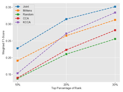
We also evaluate how our result varies with the value of selection threshold; in particular, we consider 10%, 20%, and 30%. Figure 3 shows the weighted $F_{1}$-score versus the top percentage set for the threshold in the finance domain. Our approach consistently outperforms all baselines including CCA and KCCA over different selection thresholds.

Refer to caption
Figure 3: Weighted F1-score versus top percentage of the rank set for the threshold in the finance domain.

13.3 Clinical Trial Eligibility

We study the low-data setting by restricting to only 50 observations; we use a balanced sample as in Bustos and Pertusa (2018). As before, we solve (10) for our transfer learning estimator, and solve the same objective with the Frobenius norm penalty for Mittens. In addition to using the pre-trained word embeddings of GloVe, we also use those of Word2Vec and Dict2Vec. For Word2Vec, we use the pre-trained word embeddings trained on the English CoNLL17 corpus, available at the Nordic Language Processing Laboratory (NLPL).555http://vectors.nlpl.eu/repository The pre-trained Dict2Vec embeddings are publicly available on Github.666https://github.com/tca19/dict2vec As in many semi-supervised studies, we train word embeddings using all text from both the training and test sets. In this task, we set the word embedding dimension to 100. We tune our regularization parameter $\lambda$ separately for each type of pre-trained embeddings (i.e., GloVe, Word2Vec, and Dict2Vec). We split the 50 observations into 20% for testing and 80% for training and cross-validation. We use 5-fold cross-validation to tune the hyperparameters in regularized logistic regression. Since it is computationally expensive to feed all embeddings into the model, we instead take the average of embeddings of all words in an observation as the features for the logistic regression model.

Robustness Check. Again, as described in the previous subsection, we compare with two more benchmarks CCA and KCCA, using pre-trained GloVe word embeddings. Table 13.2 shows that our transfer learning estimator still performs best compared to the two new benchmarks.

\SingleSpacedXI
Pre-trained Estimator Average F1-score
GloVe TL $\textbf{0.612554}\pm 0.003405$
Mittens $0.604338\pm 0.003413$
CCA $0.598330\pm 0.003615$
Gold $0.583299\pm 0.003516$
KCCA $0.579160\pm 0.003351$
Proxy $0.568205\pm 0.003465$
Table 13.2: F1-score of prediction over 10K trials. The 95% confidence interval is shown for each result.