Classical and quantum mixed-type lemon billiards without stickiness

Abstract

The boundary of the lemon billiards is defined by the intersection of two circles of equal unit radius with the distance $2B$ between their centers, as introduced by Heller and Tomsovic in Phys. Today 46 38 (1993). This paper is a continuation of our recent paper on classical and quantum ergodic lemon billiard ($B=0.5$) with strong stickiness effects published in Phys. Rev. E 103 012204 (2021). Here we study the classical and quantum lemon billiards, for the cases $B=0.42,\;0.55,\;0.6$, which are mixed-type billiards without stickiness regions and thus serve as ideal examples of systems with simple divided phase space. The classical phase portraits show the structure of one large chaotic sea with uniform chaoticity (no stickiness regions) surrounding a large regular island with almost no further substructure, being entirely covered by invariant tori. The boundary between the chaotic sea and the regular island is smooth, except for a few points. The classical transport time is estimated to be very short (just a few collisions), therefore the localization of the chaotic eigenstates is rather weak. The quantum states are characterized by the following universal properties of mixed-type systems without stickiness in the chaotic regions: (i) Using the Poincaré-Husimi (PH) functions the eigenstates are separated to the regular ones and chaotic ones. The regular eigenenergies obey the Poissonian statistics, while the chaotic ones exhibit the Brody distribution with various values of the level repulsion exponent $\beta$, its value depending on the strength of the localization of the chaotic eigenstates. Consequently, the total spectrum is well described by the Berry-Robnik-Brody (BRB) distribution. (ii) The entropy localization measure $A$ (also the normalized inverse participation ratio) has a bimodal universal distribution, where the narrow peak at small $A$ encompasses the regular eigenstates, theoretically well understood, while the peak at larger $A$ comprises the chaotic eigenstates, and is well described by the beta distribution. (iii) Thus the BRB energy level spacing distribution captures two effects: the divided phase space dictated by the classical Berry-Robnik parameter $\rho_{2}$ measuring the relative size of the largest chaotic region, in agreement with the Berry-Robnik picture, and the localization of chaotic PH functions characterized by the level repulsion (Brody) parameter $\beta$. (iv) Examination of the PH functions shows that they are supported either on the classical invariant tori in the regular islands or on the chaotic sea, where they are only weakly localized. With increasing energy the localization of chaotic states decreases, as the PH functions tend towards uniform spreading over the classical chaotic region, and correspondingly $\beta$ tends to $1$.

I Introduction

This paper is a continuation of our previous recent paper Č. Lozej et al. (2020) on classical and quantum ergodic billiard ($B=0.5$) with strong stickiness effects, from the family of lemon billiards introduced by Heller and Tomsovic in 1993 Heller and Tomsovic (1993). In the present paper we study lemon billiards Č. Lozej (2020a) with the shape parameters $B=0.42,\;0.55,\;0.6$, which are mixed-type billiards without stickiness regions and thus serve as ideal examples of systems with a simple divided phase space. The classical phase portraits show the structure of one large chaotic sea with uniform chaoticity (no stickiness regions) surrounding a large regular island with almost no further substructure, being entirely covered by invariant tori. The boundary between the chaotic sea and the regular island is smooth, except for a few points.

For a general introduction to the subjects in quantum chaos related to our work the reader is referred to the previous paper Č. Lozej et al. (2020). Here we only mention the introductions to the general quantum chaos in the books by Stöckmann Stöckmann (1999) and Haake Haake (2001), and the recent review papers on the stationary quantum chaos in generic (mixed-type) systems Robnik (2016, 2020).

The lemon billiards are explicitly defined in Sec. II. Recently the entire family of classical lemon billiards for a dense set of about 4000 values of $B\in[0.01,0.99975]$ (in steps of $dB=0.00025$) has been analyzed by Lozej Č. Lozej (2020a). Based on this extensive work we were able to select the interesting cases treated in this paper. The main purpose of the present paper is the analysis of the selected quantum lemon billiards $B=0.42,\;0.55,\;0.6$, with the following goals: (i) to study the energy level statistics of the entire spectrum, as well as separately of the regular and chaotic eigenstates, (ii) to calculate the Poincaré-Husimi (PH) functions of the eigenstates, analyze their structure in relationship with the classical phase portrait, and to examine the quantum localization of chaotic eigenstates and perform the analysis of their statistical properties.

The main results are the following. The level spacing distribution of the entire spectrum is well described by the Berry-Robnik (BR) distribution, if the localization of chaotic eigenstates is absent, and by Berry-Robnik-Brody (BRB) if the chaotic states are localized. Moreover, the separated regular levels obey Poissonian statistics, whilst the separated chaotic levels obey the Brody distribution exhibiting at most weak localization reflected in $\beta\approx 1$. The PH functions are found to be well supported either on invariant tori in the regular island, or on the chaotic component. The entropy localization measure of the PH functions, denoted by $A$, has a distribution with two peaks: the peak at small $A$ is associated with the regular PH functions, and is quantitatively well understood. The second peak at larger value of $A$ is associated with the chaotic PH functions and obeys the beta distribution, typical for chaotic eigenstates associated with the classical chaotic components with no stickiness (uniform ”chaoticity”). With increasing energy this beta distribution converges to a Dirac delta function peaked at the maximum value of $A=A_{0}\approx 0.7$.

The paper is organized as follows. In Sec. II we define the lemon billiards and examine their classical dynamical properties. In Sec. III we perform the statistical analysis of the energy spectra. In Sec. IV we define and calculate the Poincaré-Husimi (PH) functions and analyze their structure in relationship with the classical phase portraits. In Sec. V we introduce the entropy localization measure of the chaotic eigenstates and investigate its statistical properties. In Sec. VI we discuss the results and present the conclusions.

II The definition of the lemon billiards and their classical dynamical properties

The family of lemon billiards was introduced by Heller and Tomsovic in 1993 Heller and Tomsovic (1993), and has been studied in a number of works Lopac et al. (1999); Makino et al. (2001); Lopac et al. (2001); Chen et al. (2013); Bunimovich et al. (2016), most recently by Lozej Č. Lozej (2020a) and Bunimovich et al Bunimovich et al. (2019), and in our recent work Č. Lozej et al. (2020). The lemon billiard boundary is defined by the intersection of two circles of equal unit radius with the distance between their center $2B$ being less than their diameters and $B\in(0,1)$, and is given by the following implicit equations in Cartesian coordinates

$$(x+B)^{2}+y^{2}=1,\;\;\;x>0,$$ (1)

$$(x-B)^{2}+y^{2}=1,\;\;\;x<0.$$

As usual we use the canonical variables to specify the location $s$ and the momentum component $p$ on the boundary at the collision point. Namely the arclength $s$ counting in the mathematical positive sense (counterclockwise) from the point $(x,y)=(0,-\sqrt{1-B^{2}})$ as the origin, while $p$ is equal to the sine of the reflection angle $\theta$, thus $p=\sin\theta\in[-1,1]$, as $\theta\in[-\pi/2,\pi/2]$. The bounce map $(s,p)\Rightarrow(s^{\prime},p^{\prime})$ is area preserving as in all billiard systems Berry (1981). Due to the two kinks the Lazutkin invariant tori (related to the boundary glancing orbits) do not exist. The period-2 orbit connecting the centers of the two circular arcs at the positions $(1-B,0)$ and $(-1+B,0)$ is always stable (and therefore surrounded by a regular island) except for the case $B=1/2$, where it is a marginaly unstable orbit (MUPO), the case being ergodic and treated in our previous paper Č. Lozej et al. (2020). ${\cal L}$ is the circumference of the entire billiard given by

$${\cal L}=4\arctan\sqrt{B^{-2}-1}.$$ (2)

The area ${\cal A}$ of the billiard is equal to

$${\cal A}=2\arctan\sqrt{B^{-2}-1}-2B\sqrt{1-B^{2}}.$$ (3)

The structure of the phase space is shown in Fig. 1 for the lemon billiard $B=0.42$. The relative fraction of the area of the chaotic component of the bounce map is $\chi_{c}=0.4738$, while the relative fraction of the phase space volume of the same chaotic component is $\rho_{2}=0.4127$ (which is the Berry-Robnik parameter). The large regular island around the period-2 orbit is densely covered by the invariant tori, with no visible thin chaotic layers, and the chaotic sea is perfectly uniform, with no stickiness regions.

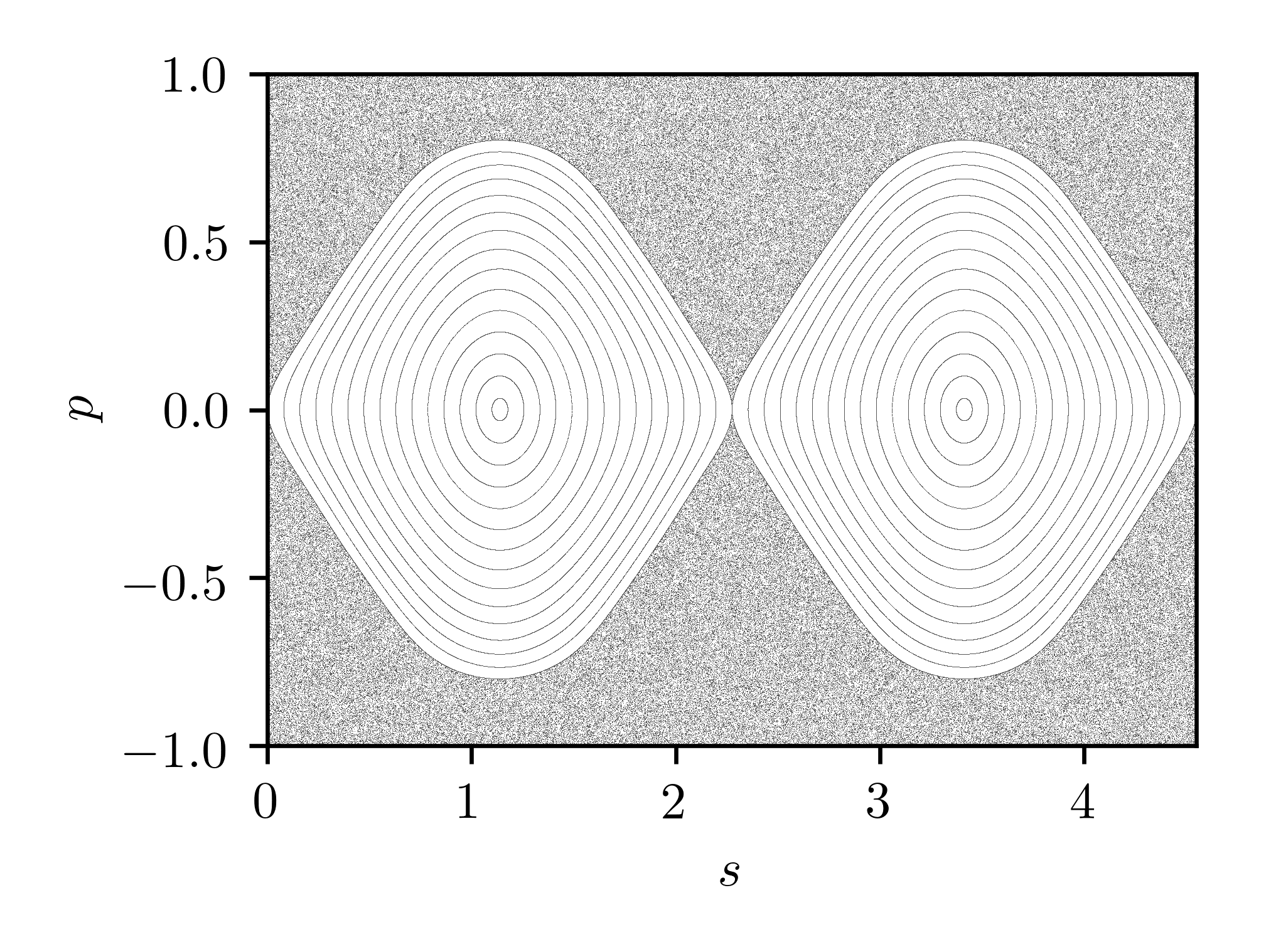
Figure 1: The phase portrait of the lemon billiard $B=0.42$. The parameters are $\chi_{c}=0.4738$, and $\rho_{2}=0.4127$, $\rho_{1}=1-\rho_{2}=0.5873$. The label on the abscissa is $s$, while on the ordinate we have $p\in[-1,1]$.

The structure of the phase space as shown in Fig. 2 for the lemon billiard $B=0.55$ is similar. The relative fraction of the chaotic component of the bounce map is $\chi_{c}=0.8204$, while the relative fraction of the phase space volume of the same chaotic component is $\rho_{2}=0.8076$.

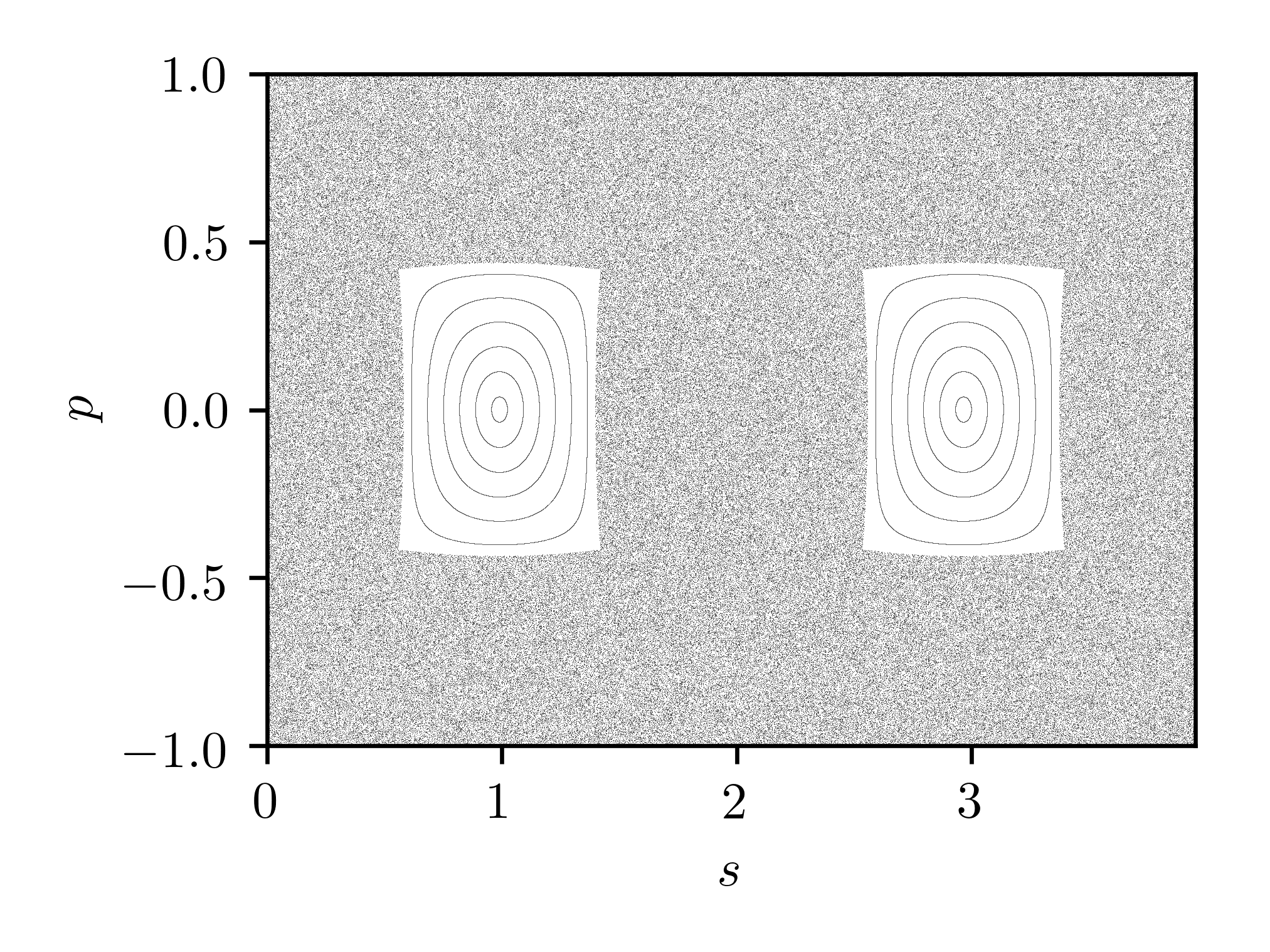
Figure 2: As in Fig. 1 but for $B=0.55$. The parameters are $\chi_{c}=0.8204$, and $\rho_{2}=0.8076$, $\rho_{1}=1-\rho_{2}=0.1924$.

Also the lemon billiard $B=0.6$ is similar as shown in Fig. 3. The relative fraction of the chaotic component of the bounce map is $\chi_{c}=0.6545$, while the relative fraction of the phase space volume of the same chaotic component is $\rho_{2}=0.6338$.

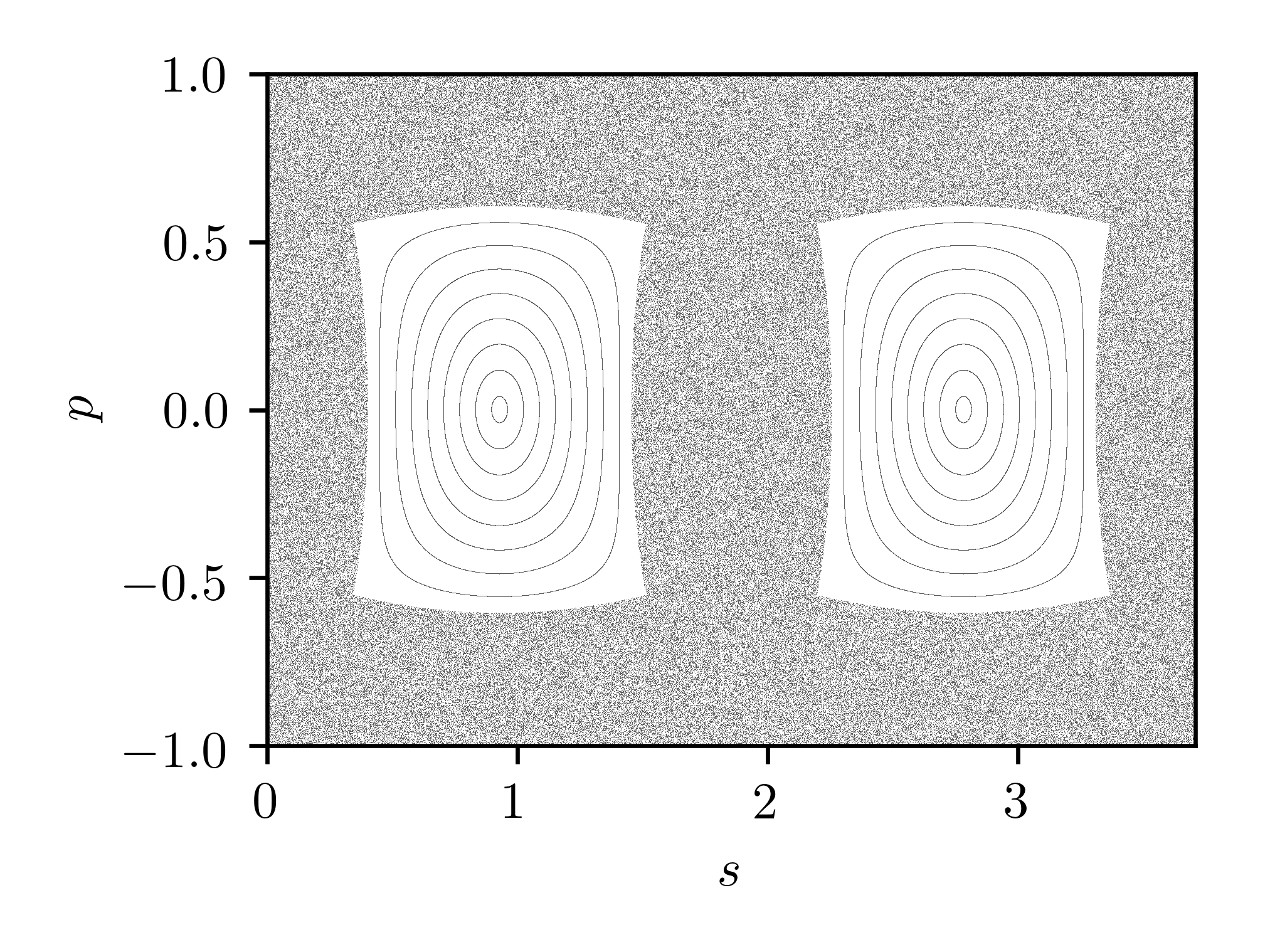
Figure 3: As in Fig. 1 but for $B=0.6$. The parameters are $\chi_{c}=0.6545$, and $\rho_{2}=0.6338$, $\rho_{1}=1-\rho_{2}=0.3662$.

We can conclude that the three cases $B=0.42,\;0.55,\;0.6$ are ideal to verify the Berry-Robnik picture of quantum billiards, including the possible quantum localization, leading to the Berry-Robnik-Brody level spacing distribution, and the universal statistical properties of the localization measures, as there are no stickiness effects, based on the results of the analysis of the recurrence time statistics in Ref. Č. Lozej (2020a), unlike in the ergodic case $B=0.5$ studied in Ref. Č. Lozej et al. (2020).

III The energy level statistics

We turn now to the quantum billiard ${\cal B}$ described by the stationary Schrödinger equation, in the chosen units ($\hbar^{2}/2m=1$) given by the Helmholtz equation

$$\Delta\psi+k^{2}\psi=0$$ (4)

with the Dirichlet boundary conditions $\psi|_{\partial{\cal B}}=0$. The energy is $E=k^{2}$.

The number of energy levels ${\cal N}(E)$ below $E=k^{2}$ is determined quite accurately, especially at large energies, asymptotically exact, by the celebrated Weyl formula (with perimeter corrections) using the Dirichlet boundary conditions, namely

$${\cal N}(E)=\frac{{\cal A}\;E}{4\pi}-\frac{{\cal L}\;\sqrt{E}}{4\pi}+c.c.,$$ (5)

where $c.c.$ are small constants determined by the corners and the curvature of the billiard boundary. Thus the density of levels $d(E)=d{\cal N}/dE$ is equal to

$$d(E)=\frac{{\cal A}}{4\pi}-\frac{{\cal L}}{8\pi\sqrt{E}}.$$ (6)

Our numerical method to solve the Helmholtz equation is based on the Heller’s plane wave decomposition method and the Vergini-Saraceno scaling method Vergini and Saraceno (1995); Č. Lozej (2020b). The numerical accuracy has been checked by the Weyl formula, to make sure that we are neither losing levels nor getting too many due to the double counting (distinguishing almost degenerate pairs from the numerical pairs) in the overlapping energy intervals, and also by the convergence test. The number of missing or too many levels was never larger than 1 per 1000 levels (usually less than 10 per 10000 levels).

Our billiard has two reflection symmetries, thus four symmetry classes: even-even, even-odd, odd-even and odd-odd. For the purpose of analyzing the spectral statistics, the wavefunctions and the corresponding PH functions, we have considered only the quarter billiard.

We have calculated the energy spectra for each billiard $B$ in nine spectral stretches starting at $k_{0}=640$ in steps of 280, namely $k_{0}=$ 640, 920, 1200, 1480, 1760, 2040, 2320, 2600, 2880, of various lengths, from 1000 levels each up to 10000 levels each. We have used the Weyl formula (5) for the spectral unfolding.

One of the most important statistical measures of the (unfolded) energy spectra is the level spacing distribution $P(S)$. For integrable systems we have Poissonian statistics and $P_{P}(S)=\exp(-S)$, while for classical ergodic (fully chaotic) systems we have Wigner distribution (Wigner surmise, which is 2-dim GOE formula), as an excellent approximation for the GOE level spacing distribution ($\infty$-dim),

$$P_{W}(S)=\frac{\pi S}{2}\exp\left(-\frac{\pi S^{2}}{4}\right).$$ (7)

There is a general very useful relationship, namely using the gap probability $E(S)$, which is the probability of having no level on an arbitrary interval of length $S$. The level spacing distribution $P(S)$ is in general equal to the second derivative of the gap probability $P(S)=d^{2}{\cal E}(S)/dS^{2}$.

For the Poisson statistics we have $E_{P}(S)=\exp(-S)$, while for the Wigner distribution we find

$${\cal E}_{W}(S)=1-{\rm erf}\left(\frac{\sqrt{\pi}S}{2}\right)={\rm erfc}\left(\frac{\sqrt{\pi}S}{2}\right).$$ (8)

In mixed-type systems we have typically one dominant chaotic component with the relative density of levels $\rho_{2}$ (equal to the relative fraction of the chaotic phase space volume), while its complement is typically a regular component of relative density $\rho_{1}=1-\rho_{2}$. If the regular and chaotic levels superimpose statistically independent of each other, then obviously the gap probability factorizes

$${\cal E}(S)={\cal E}_{P}(\rho_{1}S)\;{\cal E}_{W}(\rho_{2}S),$$ (9)

and therefore in this case the level spacing distribution is given by the Berry-Robnik formula Berry and Robnik (1984)

$$P_{BR}(S) = e^{-\rho_{1}S}e^{-\frac{\pi\rho_{2}^{2}S^{2}}{4}}\left(2\rho_{1}\rho_{2}+\frac{\pi\rho_{2}^{3}S}{2}\right)$$

$$+ e^{-\rho_{1}S}\rho_{1}^{2}{\rm erfc}\left(\frac{\sqrt{\pi}\rho_{2}S}{2}\right).$$

The above statements are true provided the Heisenberg time is larger than any classical transport time in the system Robnik (2020). If this is not the case, the chaotic eigenstates can be quantum (or dynamically) localized, which implies localized chaotic PH functions to be introduced in the next Sec. IV, and the level spacing distribution for such localized chaotic eigenstates becomes (approximately) the well known Brody distribution, Brody (1973); Brody et al. (1981), described by the following formula

$$P_{B}(S)=cS^{\beta}\exp\left(-dS^{\beta+1}\right),\;\;\;$$ (11)

where by normalization of the total probability and the first moment we have

$$c=(\beta+1)d,\;\;\;d=\left(\Gamma\left(\frac{\beta+2}{\beta+1}\right)\right)^{\beta+1}$$ (12)

with $\Gamma(x)$ being the Gamma function. It interpolates the exponential and Wigner distribution as $\beta$ goes from $0$ to $1$. The important feature of the Brody distribution is the fractional level repulsion effect, meaning the power law at small $S$, $P(S)\propto S^{\beta}$. The corresponding gap probability is

$${\cal E}_{B}(S)=\frac{1}{\gamma(\beta+1)}Q\left(\frac{1}{\beta+1},\left(\gamma S\right)^{\beta+1}\right),$$ (13)

where $\gamma=\Gamma\left(\frac{\beta+2}{\beta+1}\right)$ and $Q(a,x)$ is the incomplete Gamma function

$$Q(a,x)=\int_{x}^{\infty}t^{a-1}e^{-t}dt.$$ (14)

Here the only parameter is $\beta$, the level repulsion exponent in (11), which measures the degree of localization of the chaotic eigenstates: if the localization is maximally strong, the eigenstates practically do not overlap in the phase space (of the Wigner functions) and we find $\beta=0$ and Poissonian distribution, while in the case of maximal extendedness (no localization) we have $\beta=1$, and the GOE statistics of levels applies. Thus, by replacing ${\cal E}_{W}(S)$ with ${\cal E}_{B}(S)$ we get the so-called Berry-Robnik-Brody (BRB) distribution, which generalizes the Berry-Robnik (BR) distribution such that the localization effects are included Batistić and Robnik (2010). In this way the problem of describing the energy level statistics is empirically solved. However, the theoretical derivation of the Brody distribution for the localized chaotic states remains an important open problem. Also, while the local behaviour at small $S$, described by the power law $P(S)\propto S^{\beta}$, is certainly correct, the global feature of the Brody distribution is surely approximate, although empirically very well founded.

In our present study the classical transport time of the billiards is very short, therefore we expect $\beta\approx 1$, and the level spacing distribution is almost Berry-Robnik (III). Thus, in the level statistics we do not detect large localization effects, but accordingly, as we shall see, the PH functions still exhibit some localization manifested by the entropy localization measure $A$.

In Figs. 4-6 we show the level spacing distributions $P(S)$ for the three billiards $B=0.42,\;0.55,\;0.6$, respectively, for the spectral stretches starting at $k_{0}=2880$, for all four parities together (almost 40.000 levels), with the best fitting BRB distribution. As we see the $\beta$ parameter is very close to $1$, while the parameter $\rho_{1}$ is close to its classical value. Thus the system exhibits the Berry-Robnik picture with weak localization effects in the chaotic part of the energy spectrum, well fitted by BRB distribution. The picture is very similar for other values of $k_{0}$ listed above.

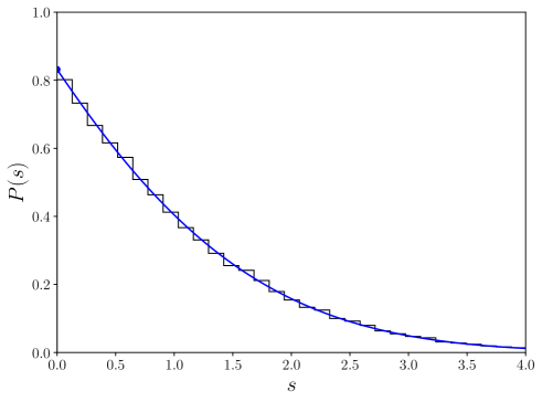
Figure 4: Level spacing distribution of the billiard $B=0.42$, for a spectral stretch starting at $k_{0}=2880$, comprising 39841 levels of all parities. The classical parameter is $\rho_{2}=0.4127$, $\rho_{1}=1-\rho_{2}=0.5873$. The blue curve is the best fitting Berry-Robnik-Brody distribution. The thick dot designates the value of $P(S=0)$. The quantum $\rho_{1}=0.590$, and $\beta=0.941$.

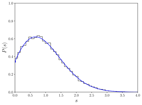
Figure 5: Level spacing distribution of the billiard $B=0.55$, for a spectral stretch starting at $k_{0}=2880$, comprising 39874 levels of all parities. The classical parameter is $\rho_{2}=0.8076$, $\rho_{1}=1-\rho_{2}=0.1924$. The blue curve is the best fitting Berry-Robnik-Brody distribution. The thick dot designates the value of $P(S=0)$. The quantum $\rho_{1}=0.189$, and $\beta=0.956$.

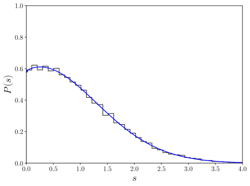
Figure 6: Level spacing distribution of the billiard $B=0.6$, for a spectral stretch starting at $k_{0}=2880$, comprising 39899 levels of all parities. The classical parameter is $\rho_{2}=0.6338$, $\rho_{1}=1-\rho_{2}=0.3662$. The blue curve is the best fitting Berry-Robnik-Brody distribution. The thick dot designates the value of $P(S=0)$. The quantum $\rho_{1}=0.356$, and $\beta=0.930$.

In Figs. 7-9 we show the dependence of the best fitting $\beta$ and $\rho_{1}$ values as functions of $k_{0}$, from $640$ to $2880$, for all four parities separately and for all of them taken together. We clearly see that the quantum value of $\rho_{1}$ agrees very well with the classical value. The value of $\beta$ is close to $1$, which indicates only weak localization of the chaotic eigenstates. The fluctuations of $\beta$ with $k_{0}$ are the strongest in case $B=0.42$, and the smallest in case $B=0.55$.

In the next sections we shall treat the PH functions and based on them will separate the regular and chaotic eigenstates, using the entropy localization measure $A$, and will show that the relative number of regular levels agrees again with the classical value $\rho_{1}$, confirming the Berry-Robnik picture.

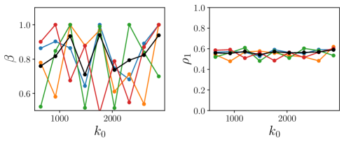
Figure 7: The billiard $B=0.42$, the best fitting $\beta$ and best fitting $\rho_{1}$ vs. $k_{0}$, based on a spectral stretch comprising about 10.000 levels for each parity, and about 40.000 of all parities. The classical $\rho_{1}=1-\rho_{2}=0.5873$. For the legend see Figs. 8 or 9.

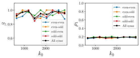
Figure 8: The billiard $B=0.55$, the best fitting $\beta$ and best fitting $\rho_{1}$ vs. $k_{0}$, based on a spectral stretch comprising about 10.000 levels for each parity, and about 40.000 of all parities. The classical $\rho_{1}=1-\rho_{2}=0.1924$.

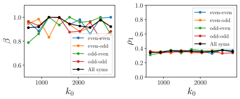
Figure 9: The billiard $B=0.6$, the best fitting $\beta$ and best fitting $\rho_{1}$ vs. $k_{0}$, based on a spectral stretch comprising about 10.000 levels for each parity, and about 40.000 of all parities. The classical $\rho_{1}=1-\rho_{2}=0.3662$.

IV The structure of Poincaré-Husimi functions

Instead of studying the eigenstates by means of the wavefunctions $\psi_{m}({\bf r})$ as solutions of the Helmholtz equation (4) we define the Poincaré-Husimi functions in the quantum phase space. PH functions are a special case of Husimi functions Husimi (1940), which are in turn Gaussian smoothed Wigner functions Wigner (1932). They are very natural for billiards. Following Tuale and Voros Tualle and Voros (1995) and Bäcker et al Bäcker et al. (2004) we define the properly ${\cal L}$-periodized coherent states centered at $(q,p)$, as follows

$$c_{(q,p),k}(s) = \sum_{m\in{\bf Z}}\exp\{i\,k\,p\,(s-q+m\;{\cal L})\}\times$$

$$\exp \left(-\frac{k}{2}(s-q+m\;{\cal L})^{2}\right).$$

The Poincaré-Husimi function is then defined as the absolute square of the projection of the boundary function $u_{m}(s)$ onto the coherent state, namely

$$H_{m}(q,p)=\left|\oint c_{(q,p),k_{m}}(s)\;u_{m}(s)\;ds\right|^{2}.$$ (16)

where $u_{m}(s)$ is the boundary function, that is the normal derivative of the eigenfunction of the $m$-th state $\psi(_{m}{\bf r})$ on the boundary at point $s$,

$$u_{m}(s)={\bf n}\cdot\nabla_{{\bf r}}\psi_{m}\left({\bf r}(s)\right).$$ (17)

Here ${\bf n}$ is a unit outward normal vector to the boundary at point ${\bf r}(s)$. The boundary function satisfies an integral equation and also uniquely determines the value of the wavefunction $\psi_{m}({\bf r})$ at any interior point ${\bf r}$ inside the billiard ${\cal B}$.

According to the principle of uniform semiclassical condensation (PUSC) of the Wigner functions and Husimi functions Robnik (1998, 2020) the PH functions are expected to condensate (collapse) in the semiclassical limit either on an invariant torus or on the chaotic component in the classical phase space.

In Figs. 10 - 11 we show examples of PH functions for the quarter billiard $B=0.42$ of even-even symmetry for six typical regular eigenstates and six typical chaotic eigenstates. Due to the double reflection symmetry and time reversal symmetry, we show only 1/8 of the phase space. The intensity of the PH functions is encoded in red, while the underlying classical phase space is plotted in grey, namely the invariant tori in the regular island, while uniformly grey region represents the chaotic sea. It is seen that regular PH functions are very well collapsed on the invariant tori, while the chaotic ones ”live” in the classically chaotic region and are localized to some extent. The degree of localization will be quantified in the next Sec. V in terms of the entropy localization measure $A$. The values of $A$ in captions of Figs. 10 - 15 are not rescaled, not divided by $\chi_{c}$ - see next Sec. V.

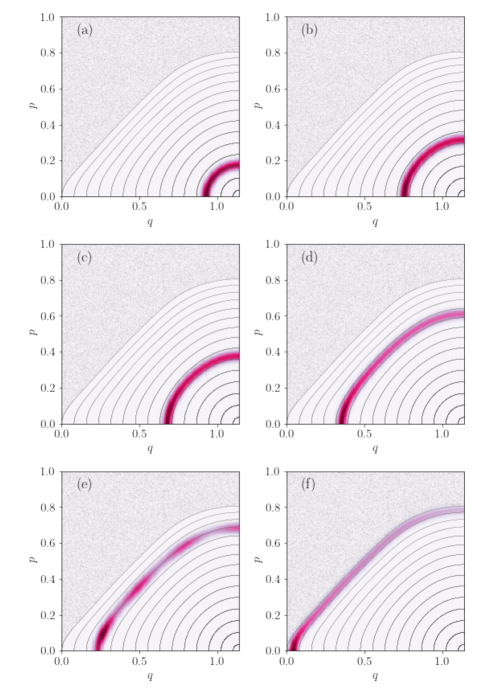
Figure 10: The billiard $B=0.42$, typical regular PH functions. We show only 1/8 of the phase space, due to the symmetries, for the even-even parity. The data $(k,A)$ are as follows from (a) to (f): (1317.630684, 0.021), (1303.594952, 0.038), (1289.244533, 0.046), (1279.769267, 0.074), (1220.262865, 0.084), (1308.380980, 0.095).

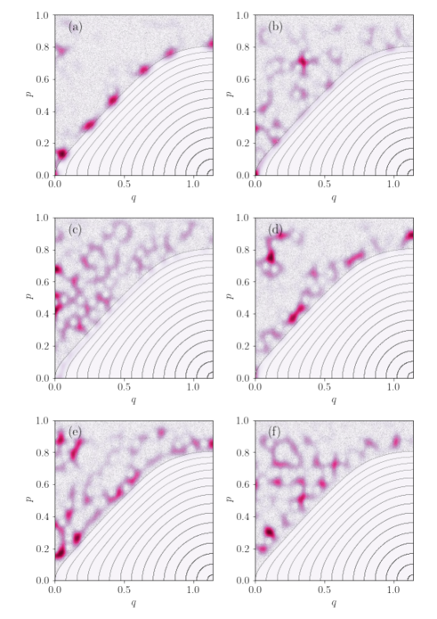
Figure 11: The billiard $B=0.42$, typical chaotic PH functions. We show only 1/8 of the phase space, due to the symmetries, for the even-even parity. The data $(k,A)$ are as follows from (a) to (f): (1220.944971, 0.220), (1321.944906, 0.323), (1245.390067, 0.371), (1215.916288, 0.269), (1274.016160, 0.294), (1293.913153, 0.296).

In Figs. 12-13 and 14-15 we show analogous results for the billiards $B=0.55,\;0.6$, respectively.

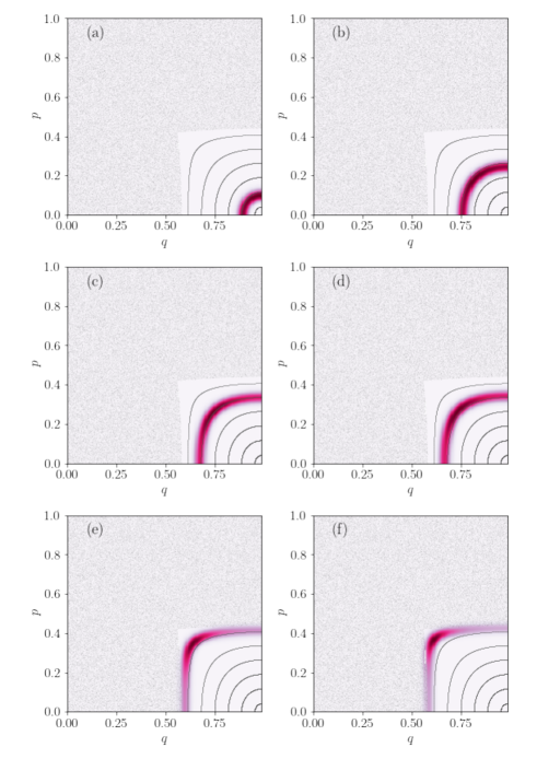
Figure 12: The billiard $B=0.55$, typical regular PH functions. We show only 1/8 of the phase space, due to the symmetries, for the even-even parity. The data $(k,A)$ are as follows from (a) to (f): (1305.660306, 0.013), (1243.133189, 0.032), (1291.780651, 0.04), (1228.988763, 0.046), (1332.681097, 0.056), (1345.816393, 0.057).

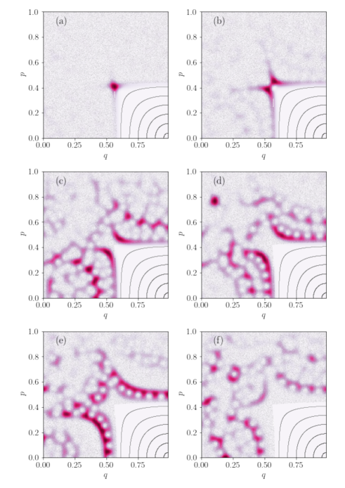
Figure 13: The billiard $B=0.55$, typical chaotic PH functions. We show only 1/8 of the phase space, due to the symmetries, for the even-even parity. The data $(k,A)$ are as follows from (a) to (f): (1345.185436, 0.304), (1351.819714, 0.382), (1358.262474, 0.520), (1298.492007, 0.446), (1312.074256, 0.454), (1377.733122, 0.481).

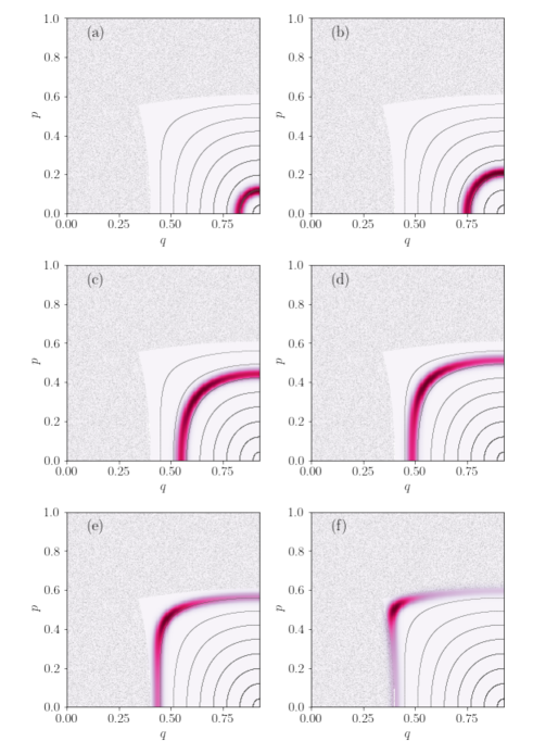
Figure 14: The billiard $B=0.6$, typical regular PH functions. We show only 1/8 of the phase space, due to the symmetries, for the even-even parity. The data $(k,A)$ are as follows from (a) to (f): (1377.224616, 0.015), (1392.401438, 0.026), (1242.886408, 0.060), (1225.928590, 0.072), (1369.637765, 0.077), (1208.778186, 0.085).

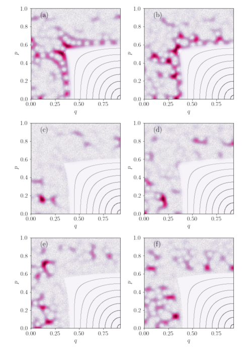
Figure 15: The billiard $B=0.6$, typical chaotic PH functions. We show only 1/8 of the phase space, due to the symmetries, for the even-even parity. The data $(k,A)$ are as follows from (a) to (f): (1315.935075, 0.406), (1323.828031, 0.406), (1307.989036, 0.329), (1267.431005, 0.383), (1370.279271, 0.364), (1275.624529, 0.392).

V The statistical properties of the entropy localization measure of PH functions

As is well known, there are at least three localization measures of chaotic eigenstates, namely the entropy localization measure $A$, the correlation localization measure $C$, and the normalized inverse participation ratio $R=nIPR$. They have been found to be linearly related and equivalent Batistić and Robnik (2013a, b); Batistić et al. (2018, 2019, 2020)

The entropy localization measure of a single eigenstate $H_{m}(q,p)$, denoted by $A_{m}$ is defined as

$$A_{m}=\frac{\exp I_{m}}{N_{c}},$$ (18)

where

$$I_{m}=-\int dq\,dp\,H_{m}(q,p)\ln\left((2\pi\hbar)^{f}H_{m}(q,p)\right)$$ (19)

is the information entropy. Here $f$ is the number of degrees of freedom (for 2D billiards $f=2$, and for surface of section it is $f=1$) and $N_{c}$ is a number of cells on the classical chaotic domain, $N_{c}=\Omega_{c}/(2\pi\hbar)^{f}$, where $\Omega_{c}$ is the classical phase space volume of the classical chaotic component. In the case of the uniform distribution (extended eigenstates) $H=1/\Omega_{C}={\rm const.}$ the localization measure is $A=1$, while in the case of the strongest localization $I=0$, and $A=1/N_{C}\approx 0$. The Poincaré-Husimi function $H(q,p)$ (16) (normalized) was calculated on the grid points $(i,j)$ in the phase space $(s,p)$, and we express the localization measure in terms of the discretized function. In our numerical calculations we have put $2\pi\hbar=1$, and thus we have $H_{ij}=1/N$ in the case of complete extendedness. $N$ is the number of grid points of the rectangular mesh with cells of equal area. In case of maximal localization we have $H_{ij}=1$ at just one point, and zero elsewhere. In all calculations we have used the grid of $200\times 400$ points, thus $N=80000$.

As is well known the localization measures of a number of consecutive eigenstates over a certain energy interval display a distribution $P(A)$. In classically ergodic systems with no stickiness $A$ obeys the beta distribution Batistić et al. (2020); Wang and Robnik (2020), while in mixed-type systems Batistić et al. (2019) it has a nonuniversal distribution with typically two peaks, as well as also in ergodic systems with strong stickiness Č. Lozej et al. (2020).

The beta distribution is

$$P(A)=CA^{a}(A_{0}-A)^{b},$$ (20)

where $A_{0}$ is the upper limit of the interval $[0,A_{0}]$ on which $P(A)$ is defined, and the two exponents $a$ and $b$ are positive real numbers, while $C$ is the normalization constant such that $\int_{0}^{A_{0}}P(A)\,dA=1$, i.e.

$$C^{-1}=A_{0}^{a+b+1}B(a+1,b+1),$$ (21)

where $B(x,y)=\int_{0}^{1}t^{x-1}(1-t)^{y-1}dt$ is the beta function.

Thus we have for the first moment

$$\left<A\right>=A_{0}\frac{a+1}{a+b+3},$$ (22)

and for the second moment

$$\left<A^{2}\right>=A_{0}^{2}\frac{(a+2)(a+1)}{(a+b+4)(a+b+3)}$$ (23)

and therefore for the standard deviation $\sigma=\sqrt{\left<A^{2}\right>-\left<A\right>^{2}}$

$$\sigma^{2}=A_{0}^{2}\frac{(a+2)(b+2)}{(a+b+4)(a+b+3)^{2}},$$ (24)

such that asymptotically $\sigma\approx A_{0}\frac{\sqrt{b+2}}{a}$ when $a\rightarrow\infty$. In this limit $P(A)$ becomes Dirac delta function peaked at $A=A_{0}$, $P(A)=\delta(A_{0}-A)$.

The maximal value of $A_{0}$ is typically empirically $A_{0}\approx 0.7$. The random wavefunction model yields $A_{0}=0.694$ Č. Lozej (2020b). It cannot be $1$, as PH function never is uniformly constant, but oscillates, and in the most chaotic random case reaches the said value $0.694$. If we compare $P(A)$ between various systems with various sizes $\chi_{c}$ of the chaotic component on the phase portrait, we must divide (normalize) the actually calculated $A$ by $\chi_{c}$.

We have done this for each of the three billiards $B=0.42,\;0.5,\;0.6$ for all nine different values of $k_{0}$. In Fig. 16 we show the $P(A)$ histograms for $k_{0}=640,\;1760,\;2880$ for the odd-odd symmetry class. We observe that $A_{0}$ is indeed close to $0.7$ in all cases. Furthermore, there are two major peaks. The left one and the right one, with an almost zero-level plateau between them. We shall see that the left peak at smaller $A$ comprises the regular eigenstates, while the right one the chaotic ones. In all cases $P(A)$ rises from $A=0$ linearly up to a maximum at $A_{c}$ (denoted by a thick red dot), then displays a sharp (almost discontinuous cut-off) drop down to zero, rises again (denoted by a thick blue diamond), reaches the minimum between the two peaks (denoted by a thick green square) and then rises again forming the second peak comprising the chaotic states. The values of the data $(A_{c},A_{0})$ from (a) to (i) are: (0.235, 0.839), (0.149, 0.747), (0.100, 0.713), (0.074, 0.742), (0.042, 0.704), (0.028, 0.703), (0.137, 0.763), (0.088, 0.733), (0.071, 0.707).

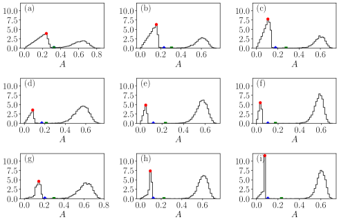
Figure 16: The histograms $P(A)$ for three billiards, $B=0.42$ (first row), $B=0.55$ (second row), and $B=0.6$ (third row), at various energies: (a,d,g) $k_{0}=640$, (b,e,h) $k_{0}=1760$, and (c,f,i) $k_{0}=2880$. The red dot denotes the maximum of the first peak at $A_{c}$, the blue diamond is the point of first increase after cut-off, and the green square denotes the minimum on the plateau between the two peaks. All states are of odd-odd parity.

This structure is quite well understood. In order to make the details more visible we show in Fig. 17 the enlarged histogram of Fig. 16(a). The linear rise of the regular peak is understood as follows. Since the thickness of the PH functions on the invariant tori (see Figs. 10, 12 and 14) is constant, their effective area and thus $A$ is proportional to the action $I$ or the length of the underlying invariant tori. The number ${\cal N}$ of eigenstates up to the given action $I$ is proportional to the area inside the regular region encircled by the given invariant torus of action $I$, thus ${\cal N}(I)\propto I^{2}$. Consequently, ${\cal N}(I)\propto A^{2}$, and its density $P(A)=d{\cal N}/dA\propto A$. The cut-off at $A_{c}$ (estimated by the value of $A$ at the maximum of the first peak) is well understood: it corresponds to the boundary of the regular region (the bordering, last invariant torus).

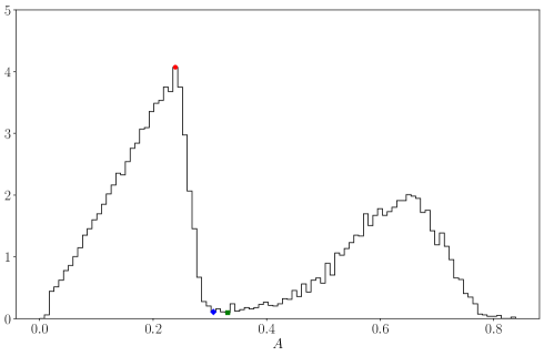
Figure 17: The enlarged histogram $P(A)$ for the billiard $B=0.42$ from Fig. 16(a). The red dot denotes the cut-off at the maximum of the first peak at $A_{c}=0.235$, the blue diamond denotes the rise again, and the green square denotes the minimum on the plateau between the two peaks. The maximal $A$ is $A_{0}=0.839$. All states are of odd-odd parity.

The regular and chaotic peaks can be separated. When this is done, we find an excellent agreement of the second peak (after normalization) with the beta distribution, like for ergodic systems without stickiness regions, demonstrated in Fig. 18.

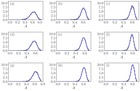
Figure 18: The histograms of the chaotic peak $P(A)$ of Fig. 16 for the billiards $B=0.42$ (first row), $B=0.55$ (second row), and $B=0.6$ (third row), at various energies: (a,d,g) $k_{0}=640$, (b,e,h) $k_{0}=1760$, and (c,f,i) $k_{0}=2880$. All states are of odd-odd parity. The agreement with the best fitting beta distribution is obvious. The parameters $(a,b)$ of the beta distribution (20) are, from (a) to (i): (20.100, 12.380), (44.209, 29.091), (59.477, 40.172), (28.982, 22.380), (52.361, 39.027), (80.315, 57.947), (31.734, 19.835), (63.872, 41.757), (90.748, 59.885).

Next we would like to understand and quantify how the histograms $P(A)$ presented in Figs. 16 tend to their semiclassical values as $k_{0}\rightarrow\infty$. The limiting form must be as follows

$$P(A)=\rho_{1}\delta(A)+\rho_{2}\delta(A_{0}-A).$$ (25)

where $\rho_{1}+\rho_{2}=1$ are the two classical parameters. For the cases of Fig. 16 we can separate the left and right peak (at the green point) and then calculate the ratio of the number of regular levels and the total number of levels in the histogram, which must agree with the classical parameter $\rho_{1}$. We find for the first row ($B=0.42$) $\rho_{1}=$ $0.5886$, $0.6032$ and $0.6102$, compared to the classical value $\rho_{1}=0.5873$, the second row ($B=0.55$) $\rho_{1}=$ $0.1924$, $0.1808$ and $0.1778$, compared to the classical value $\rho_{1}=0.1924$, and the third row ($B=0.6$) $\rho_{1}=$ $0.2912$, $0.2485$ and $0.2433$, compared to the classical value $\rho_{1}=0.3662$, which is quite satisfactory, and in agreement with the Berry-Robnik picture, except for the cases in the third row.

Finally, we would like to analyze the behaviour of $A_{c}$ and $A_{0}$ as functions of the energy, or $k_{0}$. Looking at the regular PH functions in Figs. 10, 12 and 14, we see that each PH function is uniformly spread over the invariant torus, according to PUSC, and this remains so in the (deep) semiclassical limit. Therefore the entropy localization measure $A$, which also is the effective area of the PH function, decreases linearly with the thickness of the PH function. The latter one decreases linearly with the square root of the Planck constant $2\pi\hbar$, like in the scars of Heller Heller (1984). In billiards described by the Helmholtz equation (4), using our units, the effective Planck constant is $1/k_{0}$, and thus $A_{c}$ should scale as $A_{c}\propto 1/\sqrt{k_{0}}$. A similar argument leads to the conclusion that $A_{0}$ as a function of $k_{0}$ should tend asymptotically with $k_{0}\rightarrow\infty$ to the maximum value $A_{0}=0.694\approx 0.7$, corresponding to the entirely random wavefunctions. These two observations are presented in Fig. 19, and are qualitatively and quantitatively clearly confirmed.

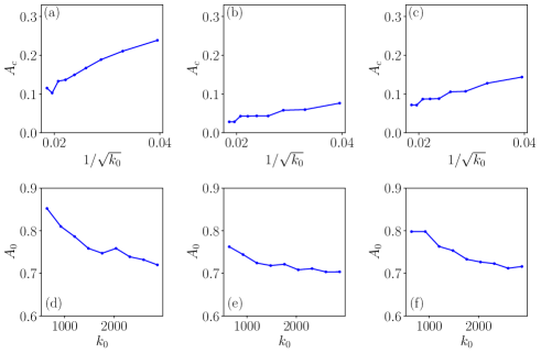
Figure 19: Top row: The cut-off value $A_{c}$ as a function of $1/\sqrt{k_{0}}$ for $B=0.42,\;0.55,\;0.6$ in (a,b,c), respectively. $A_{c}$ tends to zero with increasing $k_{0}$, linearly with $1/\sqrt{k_{0}}$. Bottom row: $A_{0}$ as a function of $k_{0}$ for $B=0.42,\;0.55,\;0.6$ in (d,e,f), respectively. $A_{0}$ tends to its limiting value $\approx 0.7$ with $k_{0}\rightarrow\infty$. Each data point refers to the distributions of $P(A)$ of all four parities.

Based on the $P(A)$ histograms like in Fig. 16, we can separate the regular and chaotic eigenstates and corresponding energy levels, the separation point beeing taken as the green square, denoting the minimum of the histogram on the plateau between the two peaks. The results are shown in Figs. 20 - 22. The behaviour in Figs. 20 - 22 is very well in agreement with the Poisson (except in Fig. 21(b)), and Brody distributions. The latter one is close to the Wigner surmise (7), since $\beta$ is close to $1$, and agrees with the value obtained from the BRB distribution, as in Fig. 5. All states are of odd-odd parity. These findings corroborate the Berry-Robnik picture of separating the regular and chaotic eigenstates Berry and Robnik (1984) in the semiclassical regime.

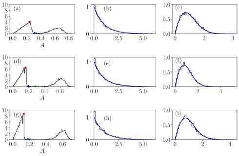
Figure 20: The level spacing distributions of separated regular (b,e,h) and chaotic levels (c,f,i), from Fig. 16, $B=0.42$, at various energies $k_{0}=640$ (a,b,c), $1760$ (d,e,f) and $2880$ (g,h,i). The quantum $\rho_{1}$ in (b,e,h) is $0.5886$, $0.6032$ and $0.6102$, to be compared to the classical value $0.5873$. The parameter values $\beta$ are (c,f,i): $0.8344$, $0.8991$ and $0.8803$, which are somewhat smaller than in Fig. 4, but compatible with Fig. 7. The full curves are the Poisson distribution and the best fitting Brody distribution. All states are of odd-odd parity.

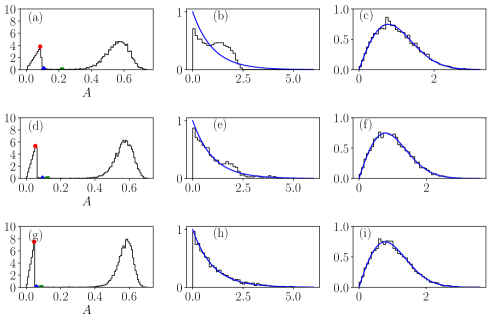
Figure 21: The level spacing distributions of separated regular (b,e,h) and chaotic levels (c,f,i), from Fig. 16, $B=0.55$, at various energies $k_{0}=640$ (a,b,c), $1760$ (d,e,f) and $2880$ (g,h,i). The quantum $\rho_{1}$ in (b,e,h) is $0.1924$, $0.1808$ and $0.1778$, to be compared to the classical value $0.1924$. The parameter values $\beta$ are (c,f,i): $0.9447$, $0.9466$ and $0.9439$, which are very close to the value in Fig. 5, and in agreement with Fig. 8. The full curves are the Poisson distribution and the best fitting Brody distribution. All states are of odd-odd parity.

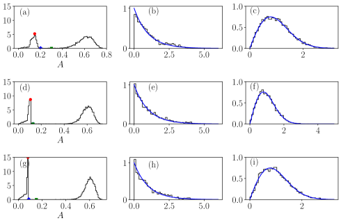
Figure 22: The level spacing distributions of separated regular (b,e,h) and chaotic levels (c,f,i), from Fig. 16, $B=0.6$, at various energies $k_{0}=640$ (a,b,c), $1760$ (d,e,f) and $2880$ (g,h,i). The quantum $\rho_{1}$ in (b,e,h) is $0.2912$, $0.2485$ and $0.2433$, to be compared to the significantly larger classical value $0.3662$. The parameter values $\beta$ are (c,f,i): $0.9447$, $0.9466$ and $0.9439$, which are close to the value in Fig. 6, and in agreement with Fig. 9. The full curves are the Poisson distribution and the best fitting Brody distribution. All states are of odd-odd parity.

One comment on the separation of eigenstates based on PH functions is necessary. Namely, there is another approach to separate the regular and chaotic eigenstates, by looking directly on the overlap of the PH functions with the classical regular and chaotic regions, respectively. This has been defined and implemented in our previous papers Batistić and Robnik (2013a, b), see also Refs. Robnik (2016, 2020). There we have introduced an overlap index $M$, which in ideal case is $1$ for chaotic states and $-1$ for regular states. In reality, in not sufficiently deep semiclassical limit, $M$ assumes also values between $1$ and $-1$, and the question arises, where to cut, at certain $M=M_{c}$. One rather ad hoc possibility is just $M_{c}=0$. But we have two possible physical criteria, (i) the classical one, and (ii) the quantum one. In the former case we choose $M_{c}$ such that the fractions of regular and and chaotic states are the classical values $\rho_{1}$ and $\rho_{2}$, respectively. The quantum criterion for $M_{c}$ is such that the fit of the chaotic level spacing distribution best agrees with the Brody distribution. This method is applicable in a general case. It turns out that the results do not depend strongly on the value of $M_{c}$, which is quite satisfactory. However, we found in the billiards considered in the present work that the results are more reliable by using the separation criterion based on $A$, in the sense that the quality of agreement with the Poisson and Brody distributions for the regular and chaotic levels, respectively, is better, and the values of $\rho_{1}$ and $\beta$ better agree with the values in Figs. 4 - 6. Of course, such a separation based on $A$ is only possible if the system possesses only one regular island embedded in a homogeneous chaotic sea with no stickiness effects, such that the regular and the chaotic peaks in the histogram $P(A)$ are well separated. These conditions are clearly satisfied in the lemon billiards $B=0.42,\;0.55,\;0.6$, so that we can take the advantage of the separation based on $A$ against the general method based on $M$.

VI Discussion and conclusions

We have demonstrated in the case of three lemon billiards $B=0.42,\;0.55,\;0.6$ with divided phase space but no stickiness regions in the chaotic sea, and no significant thin chaotic regions inside the island of regularity, that these systems are ideal for further study of mixed-type systems classically and quantally. Our main result is exploring and confirming the Berry-Robnik picture of separating statistically independent regular and chaotic eigenstates and the corresponding energy levels Berry and Robnik (1984) in the semiclassical regime. By means of Poincaré-Husimi (PH) functions we have demonstrated that indeed Principle of Uniform Semiclassical Condensation (PUSC) Robnik (1998) applies, as the PH functions clearly condense either on invariant tori, or on the chaotic component. In the latter case they can be localized as measured by the entropy localization measure $A$, but in the strict semiclassical limit become uniformly extended. The distribution of $A$ has two peaks, the regular one and the chaotic one (as for their ”population”). The former has a linear rise and a cut-off determined by the last (bordering) invariant torus, while the second one exhibits the beta distribution. In the semiclassical limit both tend to a Dirac delta function (25). A very similar analysis has recently been performed in the Dicke model Wang and Robnik (2020) describing the coupled atomic-bosonic systems, which has a classical corresponding Hamilton system with a smooth potential, which is achieved by introducing the coherent states. We believe that our present results reconfirm the evidence that much of the described scenario is typical and universal for Hamilton systems with the mixed-type (divided) phase space. If the chaotic part of the system possesses additional structure, such as strong stickiness, we find nonuniversal but very interesting behaviour as studied in the recent work Č. Lozej et al. (2020).

There are important open problems, in particular to derive by semiclassical methods the fractional power law level repulsion $P(S)\propto S^{\beta}$ at small $S$, and the corresponding empirically found (approximate) Brody distribution for the localized chaotic eigenstates. Another important open theoretical problem is to derive the beta distribution of the entropy localization measure $A$. More work is proposed in the empirical analysis of billiards and smooth Hamiltonian systems. One excellent candidate is the hydrogen atom in strong magnetic field which has important theoretical, computational, experimental and astrophysical aspects Robnik (1981, 1982); Hasegawa et al. (1989); Wintgen and Friedrich (1989); Ruder et al. (1994).

VII Acknowledgement

This paper is dedicated to the memory of our friend, outstanding scientist and organizer of science, Professor Vyacheslav Ivanovich Kuvshinov (1946-2020), the founder and permanent Editor-in-Chief of this journal, in thankfulness of his great work.

The support by the Slovenian Research Agency (ARRS) under the grant J1-9112 is gratefully acknowledged.

References

- Č. Lozej et al. (2020) Č. Lozej, D. Lukman, and M. Robnik, Phys. Rev. E 103, 012204 (2020).
- Heller and Tomsovic (1993) E. J. Heller and S. Tomsovic, Phys. Today 46, 38 (1993).
- Č. Lozej (2020a) Č. Lozej, Phys. Rev. E 101, 052204 (2020a).
- Stöckmann (1999) H.-J. Stöckmann, Quantum Chaos - An Introduction (Cambridge: Cambridge University Press, 1999).
- Haake (2001) F. Haake, Quantum Signatures of Chaos (Berlin: Springer, 2001).
- Robnik (2016) M. Robnik, Eur. Phys. J. Special Topics 225, 959 (2016).
- Robnik (2020) M. Robnik, Nonlinear Phenomena in Complex Systems (Minsk) 23, 172 (2020).
- Lopac et al. (1999) V. Lopac, I. Mrkonjić, and D. Radić, Phys. Rev. E 59, 303 (1999).
- Makino et al. (2001) H. Makino, T. Harayama, and Y. Aizawa, Phys. Rev. E 63, 056203 (2001).
- Lopac et al. (2001) V. Lopac, I. Mrkonjić, and D. Radić, Phys. Rev. E 64, 016214 (2001).
- Chen et al. (2013) J. Chen, L. Mohr, H.-K. Zhang, and P. Zhang, Chaos 23, 043137 (2013).
- Bunimovich et al. (2016) L. Bunimovich, H.-K. Zhang, and P. Zhang, Communications in Math. Phys. 341, 781 (2016).
- Bunimovich et al. (2019) L. A. Bunimovich, G. Casati, T. Prosen, and G. Vidmar, Experimental Mathematics 1, 10 (2019).
- Berry (1981) M. V. Berry, Eur. J. Phys. 2, 91 (1981).
- Vergini and Saraceno (1995) E. Vergini and M. Saraceno, Phys. Rev. E 52, 2204 (1995).
- Č. Lozej (2020b) Č. Lozej, Ph.D. Thesis, University of Maribor (2020b).
- Berry and Robnik (1984) M. V. Berry and M. Robnik, J. Phys. A: Math. Gen. 17, 2413 (1984).
- Brody (1973) T. A. Brody, Lett. Nuovo Cimento 7, 482 (1973).
- Brody et al. (1981) T. A. Brody, J. Flores, J. B. French, P. A. Mello, A. Pandey, and S. S. M. Wong, Rev. Mod. Phys. 53, 385 (1981).
- Batistić and Robnik (2010) B. Batistić and M. Robnik, J. Phys. A: Math. Theor. 43, 215101 (2010).
- Husimi (1940) K. Husimi, Proc. Phys. Math. Soc. Jpn. 22, 264 (1940).
- Wigner (1932) E. Wigner, Phys. Rev. 40, 749 (1932).
- Tualle and Voros (1995) J. Tualle and A. Voros, Chaos Solitons Fractals 5, 1085 (1995).
- Bäcker et al. (2004) A. Bäcker, S. Fürstberger, and R. Schubert, Phys. Rev. E 70, 036204 (2004).
- Robnik (1998) M. Robnik, Nonlinear Phenomena in Complex Systems (Minsk) 1, 1 (1998).
- Batistić and Robnik (2013a) B. Batistić and M. Robnik, Phys. Rev. E 88, 052913 (2013a).
- Batistić and Robnik (2013b) B. Batistić and M. Robnik, J. Phys. A: Math. Theor. 46, 315102 (2013b).
- Batistić et al. (2018) B. Batistić, Č. Lozej, and M. Robnik, Nonlinear Phenomena in Complex Systems (Minsk) 21, 225 (2018).
- Batistić et al. (2019) B. Batistić, Č. Lozej, and M. Robnik, Phys. Rev. E 100, 062208 (2019).
- Batistić et al. (2020) B. Batistić, Č. Lozej, and M. Robnik, Nonlinear Phenomena in Complex Systems (Minsk) 23, 17 (2020).
- Wang and Robnik (2020) Q. Wang and M. Robnik, Phys. Rev. E 102, 032212 (2020).
- Heller (1984) E. J. Heller, Phys. Rev. Lett. 53, 1515 (1984).
- Robnik (1981) M. Robnik, J. Phys. A: Math. Gen. 14, 3195 (1981).
- Robnik (1982) M. Robnik, J. Phys. Colloque C2 43, 29 (1982).
- Hasegawa et al. (1989) H. Hasegawa, M. Robnik, and G. Wunner, Prog. Theor. Phys. Suppl. (Kyoto) 98, 198 (1989).
- Wintgen and Friedrich (1989) D. Wintgen and H. Friedrich, Phys. Rep. 183, 38 (1989).
- Ruder et al. (1994) H. Ruder, G. Wunner, H. Herold, and F. Geyer, Atoms in Strong Magnetic Fields (Heidelberg: Springer, 1994).