Feasibility of Primordial Black Hole Remnants as Dark Matter
in View of Hawking Radiation Recoil

Abstract

It has recently been suggested that black hole remnants of primordial origin are not a viable dark matter candidate since they would have far too large a velocity due to the recoil of Hawking radiation. We re-examined this interesting claim in more details and found that it does not rule out such a possibility. On the contrary, for models based on non-commutativity of spacetime near the Planck scale, essentially the same argument can be used to estimate the scale at which the non-commutativity effect becomes important. If dark matter “particles” are non-commutative black holes that have passed the maximum temperature, this implies that the non-commutative scale is about 100 times the Planck length. The same analysis applies to other black hole remnants whose temperature reaches a maximum before cooling off, for example, black holes in asymptotically safe gravity.

I Black Hole Remnants as Dark Matter Candidate

Dark matter, a mysterious component in our Universe that contributes additional gravitational pull and is essential for structure formation, remains elusive even after decades of efforts to pin down its identity. Theorists have proposed a plethora of dark matter candidates, ranging from various weakly interacting massive particles (WIMPs) to the attempts to do away with actual dark matter by modifying general relativity (which is a nontrivial task [1]). Yet another possibility is that dark matter actually consists of microscopic primordial black holes. Of course, there could be many types of dark matter, so these possibilities are not mutually exclusive.

Primordial black holes [2] can be created from fluctuations in the early Universe [3, 4, 5, 6]. They may also be the result of phase transitions in the early Universe [7, 8, 9], or induced by inflation [10, 11, 12, 13, 14, 14, 15, 16, 17, 18, 19, 20]. Indeed the possibility of primordial black holes playing the role of cold dark matter has been discussed extensively in the literature [21, 22, 23, 24, 25, 26, 27], and observational constraints from various approaches are now available [28, 29, 30, 31, 32]. See also [33, 34, 35, 36, 37, 38] for future observational prospects. Notably, if dark matter consists of (entirely or mainly) primordial black holes, then the corresponding gravitational waves induced by non-Gaussian scalar perturbations are detectable by LISA-like detectors with some distinguishable features [40]. The fraction of primordial black holes contributing to dark matter can also be constrained by measuring (anti)neutrino signals at the large liquid-scintillator detector of Jiangmen Underground Neutrino Observatory (JUNO) [41]. Intriguingly, the NANOGrav results are consistent with possible signals from primordial black holes [43, 44, 45]. Due to quantum gravitational corrections, it is possible that Hawking radiation either completely stops or slows down considerably for these black holes so they do not completely evaporate once they reach a certain size around the Planck scale. These are called black hole remnants [21, 46].

Recently, Kováčik [47] argued that microscopic black holes gain large velocities from the recoil of Hawking emissions and as such they would not be a feasible cold dark matter candidate (“cold” means that their velocity is small). Indeed, as black holes evaporate due to Hawking radiation, they will recoil due to the conservation of linear momentum. Such an effect, accumulated over the typically long lifetime of an astrophysical black holes has been known to cause the position of the black holes to drift across space in the style of a random walk [50, 51]. The argument in [47] is to consider some models in non-commutative spacetime in which the Schwarzschild-like black hole is essentially Schwarzschild at large enough mass, but its Hawking temperature eventually reaches a maximum, $T_{m}$, when the size of the black hole is sufficiently small. Afterwards the temperature continues to drop towards zero as the mass progressively decreases. Thus eventually the black hole becomes an extremal remnant with no further emission of particles. Crucially, the temperature as a function of the mass grows and falls considerably around the peak.

Working in the units $G=c=\hbar=1$ (and sign convention $(-,+,+,+)$), we denote the mass of the black hole at its maximum temperature by $M_{m}$ and that of the final remnant mass by $M_{0}$. Due to the appreciable rise and drop of the temperature curve around the maximum, the total number of quanta emitted as the black hole evaporates from mass $M_{m}$ to $M_{0}$ is relatively small [47]: $N\sim(M_{m}-M_{0})/T_{m}\lesssim 100$. Each quantum carries a momentum $p\sim(M_{m}-M_{0})/N$, so after radiating $N$ particles the black hole receives a momentum recoil of $(M_{m}-M_{0})/\sqrt{N}$ by the standard random walk argument. The final velocity of the black hole remnant is then

$$v_{r}\approx\frac{M_{m}-M_{0}}{M_{0}\sqrt{N}}.$$ (1)

It was estimated in [47] that the velocity is high $\left(\mathcal{O}(0.01)\right.$ to $\mathcal{O}(0.1)$ of the speed of light, depending on the models$\left.\right)$, which is far too large for these black holes to qualify as cold dark matter.

In this work, we wish to argue that while the calculation is essentially correct, it does not rule out primordial black hole remnants as a possible viable dark matter candidate. There are a few reasons for this: Firstly, the non-commutative models come with the so-called non-commutative parameter, which dictates when non-commutativity effect becomes apparent. As will be discussed in Sec.(II), the parameter is constrained by observations, and need not be taken to be equal to the Planck length as was done in [47]. Indeed, we could turn this argument around and use the expected dark matter speed to deduce the non-commutative parameter. In fact, this is our main motivation – to estimate the scale at which quantum gravitational effect might become important, by making contacts with observations. Secondly, the whole dynamics and time scale of the Hawking evaporation should be taken into account: if the initial mass of the black hole is large enough, it may not have enough time to evolve past the temperature peak. Furthermore, since the remnant has zero temperature, most likely the evaporation time scale from the temperature peak to zero temperature would take an infinite amount of time, which is to be expected from the third law of black hole thermodynamics. Lastly, this argument does not apply to models in which the black hole remnant stops evaporating at the maximum temperature, that is $M_{m}=M_{0}$, such as the GUP (generalized uncertainty principle)-corrected Schwarzschild black hole [52].

Let us now examine in details one of the non-commutative black hole models and comment more on the points mentioned above. More models are further explored in the Appendix.

II Primordial Black Holes as Dark Matter in Non-Commutative Models

As explained in [53], it is not possible to measure with arbitrary precision small volume of space arbitrary precisely. Any attempt to measure physical properties in a region of about the Planck size would involve so much energy that the local geometry should fluctuate significantly and therefore cause black holes (or other more exotic objects such as wormholes) to form. Intuitively one can understand this as a consequence of the uncertainty principle: if $\Delta x$ is small then $\Delta p$ of the probe (say, a light pulse) must be large. The energy $\Delta E=\Delta p\cdot c$ is therefore also large, and huge amount of energy fluctuation in a sufficiently small region would lead to black hole formation.

One possible mathematical model to implement such an idea geometrically is the so-called non-commutativity spacetime (see the review [54, 55, 56, 57]): at around the Planck scale, the spatial coordinates of the spacetime manifolds are subjected to the non-commutativity effect:

$$\left[\hat{x_{i}},\hat{x_{j}}\right]=2iL\hat{x_{k}}\epsilon^{ijk},$$ (2)

where $\epsilon^{ijk}$ is the Levi-Civita symbol and $L=\lambda\ell_{\text{P}}$ is the length scale of non-commutativity. Non-commutativity is not just an ad hoc proposal – it is well motivated from more fundamental quantum gravity theories such as string theory [58, 59]. Since the effects of non-commutativity have not been observed in the experiments done so far, the parameter $L$ must satisfy the constraint $L<10^{-18}$ m [60]. See also [61], in which the parameter $L$ is argued to be around $10^{-21}-10^{-23}$ m by considering gamma ray burst (GRB) data (since non-commutativity can influence the group velocity of massless particle wave packets). The latter bound is only indicative of the upper bound due to uncertainties of the spectral lack and the GRB statistics.

Mathematically one could formally treat the mass of the Schwarzschild black hole in general relativity as being “localized” at the “origin” $r=0$, i.e. supported by a delta function. This is only a formality because the origin is spacelike and lies in the future of any observer. In the case of non-commutative spacetime, the “source” of the black hole is no longer sharply localized in spacetime by a delta function; rather, we need to use a matter density distribution that is centered in the origin. A possible distribution function is given by

$$\rho(r)=\rho_{0}e^{-\left[r/(\alpha L)\right]^{\alpha}},$$ (3)

where $\alpha=1,2,3$ is a parameter determining which model we are considering and $\rho_{0}$ also depends on the model. The density in (3) reproduces a delta function in the limit $\lambda\to 0$.

Let us start with the $\alpha=2$ model described in [60]. The models with $\alpha=1$ and $\alpha=3$ are similar and are shown in the appendix for completeness. From now on, we shall use natural units except where explicitly specified.

The density in (3) in this case is given by

$$\rho(r)=\frac{M}{(2\lambda\sqrt{\pi})^{3}}e^{-\left[r/(2\lambda)\right]^{2}}.$$ (4)

One considers a spherically symmetric Schwarzschild-like metric and imposes the conditions : $g_{00}=-g_{rr}^{-1}$ and $T_{r}^{r}=T^{0}_{0}=-\rho(r)$ on the energy-momentum tensor. We can thus write the metric in the form: $g=\text{diag}\left(f(r),-f(r)^{-1},r^{2},r^{2}\sin(\theta)\right)$. The $00$-component of the Einstein equations thus gives an equation for $f(r)$:

$$\frac{1+f(r)+f^{\prime}(r)}{r^{2}}=8\pi T_{00}=\frac{4M}{\lambda^{3}\sqrt{\pi}}e^{-\left[r/(2\lambda)\right]^{2}}.$$ (5)

The solution of this equation is:

$$f(r)=-1+\frac{4M}{\sqrt{\pi}r}\gamma\left(\frac{3}{2},\frac{r^{2}}{4\lambda^{2}}\right),$$ (6)

where $\gamma\left(3/2,r^{2}/(4\lambda^{2})\right)$ is the lower incomplete Gamma function defined as:

$$\gamma\left(\frac{3}{2},\frac{r^{2}}{4\lambda^{2}}\right):=\int_{0}^{\frac{r^{2}}{4\lambda^{2}}}e^{-t}\sqrt{t}\operatorname{d}\!{t}.$$ (7)

The event horizon is located at the root of $g_{rr}=0$, i.e., at $f(r)=0$, corresponding to:

$$r_{H}=\frac{4M}{\sqrt{\pi}}\gamma\left(\frac{3}{2},\frac{r_{H}^{2}}{4\lambda^{2}}\right).$$ (8)

This equation has to be solved numerically by plotting $f(r)$ and observing its intersections with the $r$ axis.

Figure 1: $-f(r)$ as a function of the coordinate radius, in units of $\lambda$ for $M=M_{0}$, $M=2/3$ $M_{0}$, and $M=3/2$ $M_{0}$.

Here three cases are represented, corresponding to zero, one or two intersections with the $r$ axis. These possibilities are discriminated by a minimal mass $M_{0}$, below which there is no event horizon. It can be shown (see [60]) that if $M<M_{0}$ there are no naked singularity, despite there being no horizons. The trace of the Einstein equations gives the curvature scalar:

$$R(0)=\frac{4M}{\sqrt{\pi}\lambda^{3}},$$ (9)

which is nowhere divergent, including at $r=0$. From the equation for $f(r)$ (6) we can also calculate the Hawking temperature in the usual way:

$$T=-\left(\frac{1}{4\pi}\frac{\operatorname{d}\!{g}_{00}}{\operatorname{d}\!{r}}\right)_{r_{H}}.$$ (10)

Using the expression (8) to re-express $M$, we obtain:

$$T=\frac{1}{4\pi r_{H}}\left[1-\frac{r_{H}^{3}e^{-\frac{r_{H}^{2}}{4\lambda^{2}}}}{4\lambda^{3}\gamma\left(\frac{3}{2},\frac{r_{H}^{2}}{4\lambda^{2}}\right)}\right].$$ (11)

The temperature can now be plotted in units of $\lambda$, giving the result in Fig.(2).

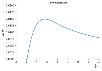
Figure 2: Temperature as a function of the radius, in units of $\lambda$.

We note that zero temperature corresponds to $r_{0}$, since it is the minimum of $-g_{00}$ (see figure 1), implying $\operatorname{d}\!{g}_{00}/\operatorname{d}\!{r}=0$ in $r_{0}$. For $r_{H}<r_{0}$ there is no horizon and thus the $T$ in Eq.(11) cannot be defined. We can see the numerical results in Table 1, expressed in the Planck units.

$M_{0}$ :	$\left(1.6874815942\right.$	$\pm$	$\left.10^{-10}\right)$	$\lambda$
$r_{0(H)}$ :	$\left(3.02243\right.$	$\pm$	$\left.10^{-5}\right)$	$\lambda$
$r_{0(T)}$ :	$\left(3.0596813\right.$	$\pm$	$\left.10^{-7}\right)$	$\lambda$
$T_{m}$ :	$\left(1.4934245\right.$	$\pm$	$\left.10^{-7}\right)10^{-2}$	$1/\lambda$
$r_{m}$ :	$\left(4.7663222\right.$	$\pm$	$\left.10^{-7}\right)$	$\lambda$
$M_{m}$ :	$2.41$			$\lambda$

Table 1: The values of $r_{0(H)}$ and $M_{0}$ are calculated numerically from Fig.(1), while $r_{0(T)}$ is obtained from Fig.(2). The latter result is different from $r_{0(H)}$, but more precise and convenient to solve for since Eq.(11) only involves $r_{H}$ and $\lambda$, whereas Eq.(8) involves also $M$. We suspect this discrepancy is due to the presence of the incomplete gamma function in the numeric (as this does not arise in the models with $\alpha=1$ and $\alpha=3$ discussed in the appendix), but in any case this does not affect our qualitative discussions. The value $M_{m}$ is obtained analytically from Eq.(8).

Another feature of the peak temperature is the recoil velocity, as analysed in [62] for the $\alpha=1$ model. As explained briefly in Sec.(I), the argument is that a number of quanta is emitted as the black holes evolve from the temperature peak to $T=0$, which spans a relatively narrow range of the mass, thus giving a huge recoil velocity to the black holes. Restoring the physical constants, the number of quanta in SI units is:

$$N_{q}\sim\frac{c^{2}(M_{m}-M_{0})}{T_{m}k_{B}}\approx 48\lambda^{2},$$ (12)

where $k_{B}$ is the Boltzmann constant and the masses and temperature used above are the values taken from the Table 1 multiplied by the Planck mass and Planck temperature respectively. Then, we get $N_{q}\approx 48$ if we choose $\lambda=1$ ($L$ is the Planck length $\ell_{\text{P}}$). Calculating the momentum of the emitted quanta as the result of a random walk process, we get the following expression for the recoil velocity of the black hole:

$$v_{r} =\frac{M_{m}-M_{0}}{M_{0}\sqrt{N_{q}}}c=\frac{\sqrt{\left(M_{m}-M_{0}\right)T_{m}k_{B}}}{M_{0}}$$

$$\approx 1.85\cdot 10^{7}\frac{1}{\lambda}~{}\text{ms}^{-1}.$$ (13)

The conversion of the masses and temperature is obtained exactly as done before. Choosing $L=\ell_{\text{P}}$ gives $v_{r}\approx 1.85\times 10^{4}$ km/s, which is far too large to be a cold dark matter candidate. Indeed, in [63], the circular velocity of dark matter in our galaxy is estimated to be around $218-246$ km/s. If our result is to be comparable with this, then it would require choosing $L\sim 10^{2}\ell_{\text{P}}$.

At this point, one might wonder why we do not consider the speed caused by the recoil as the black hole evaporates from its initial mass down to $M_{m}$. This is because the speed in this period is negligible. In the model of [51] for example, it was shown that the speed of a recoiled Schwarzschild black hole is roughly the inverse of the initial mass for most part of the evolution until the last moments of the evaporation. This is due to the fact that the momentum is set by the temperature scale, and as the temperature becomes unbounded towards the end, one can show that the velocity, which is related to the speed via $p=\gamma mv$ in the relativistic regime, will asymptote to the speed of light. In the non-commutative case discussed here, however, the maximum temperature occurs way before Planck temperature, and so the speed is negligible for most part of the evolution before $M_{m}$ is reached.

Now, according to [54] and [64], if the Hawking temperature of a black hole reaches $T\approx 2.7$ K at the current epoch, it will attain thermal equilibrium with the cosmic microwave background (CMB) photons and thus stop evaporating. While this may be true for larger black holes, it is not what happens in our case when the black holes are microscopic. Indeed, even if the black hole and the universe share the same temperature, they are not actually in thermal equilibrium. This is due to the scattering cross section $\sigma\sim\pi r_{0}^{2}\approx 28$ $\lambda^{2}$, corresponding to $7.38\times 10^{-69}$ $\lambda^{2}$ $\text{m}^{2}$ in SI units, that is too small for any effective interaction with the CMB radiation. If we want $\sigma$ to be of the order of the Thomson cross section $\sigma_{T}\approx 6.6\times 10^{-29}$ $\text{m}^{2}$, we would need $L\sim 10^{20}$ $\ell_{\text{P}}$, which exceeds even the lower end of the phenomenological constraint $L<10^{-18}$ m. Therefore, we can conclude that the evaporation of non-commutative black hole would continue as it approaches the asymptotic extremal state $T=0$ and $M=M_{0}$. Expressing this mass in SI units, it is $M_{0}=3.67\times 10^{-8}$ $\lambda$ kg. This value is a little larger than $M_{\text{P}}$ (the Planck mass) even for $\lambda=1$, so the remnants left by the evaporation, though the same order, are not exactly Planckian.

Now let us see whether primordial black holes (PBHs) could be found around the temperature peak in our present epoch. The mass corresponding to the peak temperature, when the constants are restored, is $M_{m}=2.41$ $\lambda M_{\text{P}}$. In SI units, we have $M_{m}=5.25\times 10^{-8}$ $\lambda$ kg. Following [65], black holes with initial masses larger than $10^{15}$ g would stay essentially the same throughout their lifetime and the more massive ones can even be accreted. In fact, the time scale for evaporation is even slightly longer if one takes into account the sparsity of the radiation [66]. Thus, this kind of black holes would be too far from the peak for any allowed value of the parameter $\lambda$.

On the contrary, PBHs with initial masses equal or smaller than the critical mass $M_{cr}=5.1\times 10^{14}$ g can evaporate effectively [65]. If the mass is around $M_{cr}$, the PBH is expected to have evaporated to around $M_{0}$ by the present epoch (assuming general relativity holds). Therefore, for a quick estimate, taking a slightly higher initial mass means the black hole could be located near the temperature peak if there is a non-commutativity correction. The value of $\lambda$ in its range of validity does not affect substantially the initial mass $M_{i}\sim M_{cr}$ and so we are free to set $\lambda\sim 10^{2}$ to match the velocity of dark matter. Black holes with initial masses lower than $M_{cr}$, would be well on their way to become extremal remnants of mass $M_{0}$.

The bottom line is that the model comes with a non-commutativity scale $\lambda$, the value of which can be inferred from the dark matter velocity if the primordial non-commutative black holes are indeed dark matter particles. We also check the model with $\alpha=1$ and $\alpha=3$ in the Appendix and find the same conclusion holds.

III Conclusion: Microscopic Primordial Black Holes Remain Feasible as Dark Matter Candidate

In this work we have shown that primordial black holes remain a viable dark matter candidate. The argument in [65] that microscopic black holes gain too large a velocity towards the end of Hawking evaporation (and therefore cannot behave as cold dark matter) of course depends on the underlying models of quantum gravity phenomenology. Specifically it only applies to those models in which the Hawking temperature of a Schwarzschild-like black hole turns around near the end of the Hawking evaporation, such as the models that employ non-commutative spacetime. Even then, this is true only for some values of the non-commutative parameter $\lambda$, and is only relevant if the initial mass of the black hole is small enough – for otherwise it would not have enough time to evolve past the temperature peak.

We show that it is possible to choose $\lambda$ such that microscopic black holes that have passed the temperature peak still have velocity that is consistent with dark matter, as required from astrophysical observations. In this simple analysis following the method in [47], the value of $\lambda$ turns out to be at the order of $\mathcal{O}(10^{2})$ (this is also the case for the other non-commutative models explored in the appendix, so it is somewhat robust), which is still within the observational constraint of not having detected a non-commutative spacetime geometry. Interestingly, this is consistent with the argument in [61] that the scale of non-commutativity could be larger than the Planck length.

In a more careful analysis, the time it takes for a black hole to evolve from $M_{m}$ (the mass corresponding to the temperature peak) to $M_{0}$ (the final remnant mass) should be taken into account by solving the evolution equation of $\operatorname{d}\!{M}/\operatorname{d}\!{t}$, though this is not quite feasible in these models since the expression for the horizon cannot be readily obtained. Since the final remnant has zero temperature, the evaporation time from the peak to the final state would likely take an infinite amount of time. In fact, as the temperature drops, the evaporation process becomes slower and slower. This mean that the recoil velocity might be of the form

$$v_{r}\approx\frac{M_{m}-M_{*}}{M_{*}\sqrt{N}}=\frac{\sqrt{(M_{m}-M_{*})T_{m}}}{M_{*}},$$ (14)

where $M_{*}>M_{0}$ is the current mass of the black hole. We note that $v_{r}$ is a decreasing function of $M_{*}$ for fixed $M_{m}$. Therefore, there is a value near the maximum $M_{m}$ where it is of the same order of magnitude as the observed velocity, for $\lambda=1$. For $M_{*}$ even larger than this value (but still less than $M_{m}$), this would imply that the recoil velocity could be considerably smaller than expected even if we take the length scale $L$ to be closer to the Planck length.

Since astrophysical black holes have angular momentum, and could be charged (not necessarily by ordinary Maxwell field, but conceivably by some hidden U(1) field related to the dark sector), one might wonder whether our conclusions would need to be revise substantially if these effects are included. We think that this is unlikely. Charged black holes in the presence of spacetime non-commutativity had been studied by Alavi [68]. We can repeat our calculation using the charged metric and indeed the qualitative results remain unchanged. From the work of Nicolini and Modesto [69] we can also argue that when rotation is included, the result is also qualitatively the same. See also [70], in which Paik discussed how the angular momentum and charge are lost as we approach the non-commutativity scale. In other words, charge and angular momentum do not affect the conclusion by much at this scale (they would certainly be important when the black holes are still at the astrophysical scale, and the exact evolution up to near Planck scale would require much detailed modeling).

In any case, we conclude that recoil speed due to Hawking radiation does not rule out primordial microscopic black holes as a dark matter candidate. Finally we remark that the analysis and discussion in this work is not only applicable to the non-commutative black hole models but also to all other quantum gravitational inspired models as long as the microscopic black holes have a temperature peak and a turnover of the temperature after the peak (whether the end state is some finite temperature state or zero temperature state is not so crucial). One such example is the Schwarzschild-like black hole in asymptotically safe gravity [71, 72], which we also briefly discuss in the Appendix.

Appendix

In this Appendix we shall repeat the calculation in Sec.(II) for the models in which $\alpha=1$ and $\alpha=3$, respectively. The results for both cases are essentially the same with that of $\alpha=2$ discussed above. Nevertheless it might be useful for future references to have the explicit results shown.

.1 Model with $\alpha=1$

An alternative model, obtained by taking $\alpha=1$ in the density function (3), has been investigated in [47] and [62]. The density is given by

$$\rho(r)=\frac{M}{(2\lambda)^{3}\pi}e^{-r/\lambda}.$$ (15)

Proceeding analogously as the $\alpha=2$ model and requiring the metric to be Schwarzschild-like and spherically symmetric, we calculate the $00$-component of the Einstein equations:

$$\frac{1+f(r)+f^{\prime}(r)}{r^{2}}=8\pi T_{00}=\frac{M}{\lambda^{3}}e^{-r/\lambda},$$ (16)

where $g_{00}=f(r)=-g_{rr}^{-1}$ and $T^{0}_{0}=-\rho(r)$. The solution of the above equation is:

$$f(r)=-1+\frac{2M}{r}-\frac{M}{r}e^{-\frac{r}{\lambda}}\left(\frac{r^{2}}{\lambda^{2}}+\frac{2r}{\lambda}+2\right).$$ (17)

The event horizon is located at $g_{rr}=0$, i.e., at $f(r)=0$. To find this value, it is again necessary to plot $f(r)$ and compute numerically its intersections with the $r$ axis:

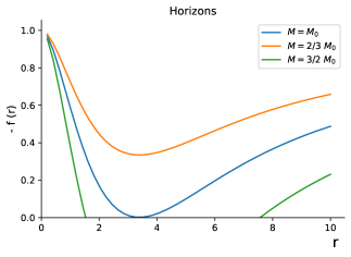
Figure 3: $-f(r)$ as a function of the radius, in units of $\lambda$ for $M=M_{0}$, $M=2/3$ $M_{0}$, $M=3/2$ $M_{0}$.

We notice again that there are three cases: zero, one or two intersections with the $r$ axis, corresponding to $M$ less, equal or greater than the minimal mass $M_{0}$. From Eq.(17), the Hawking temperature is given by

$$T=-\left(\frac{1}{4\pi}\frac{\operatorname{d}\!{g}_{00}}{\operatorname{d}\!{r}}\right)_{r_{H}}.$$ (18)

From the same equation, Eq.(17), we can also derive an expression for $M(r_{H})$ when $f(r)=0$ and substitute it in the temperature equation. The end result is:

$$\lambda T=\frac{1}{4\pi x}\frac{x^{3}+x^{2}+2x-2\left(e^{x}-1\right)}{x^{2}+2x-2\left(e^{x}-1\right)},$$ (19)

where $x=r_{H}/\lambda$. The plot of the temperature, expressed in units of $\lambda$, is given in Fig.(4) below.

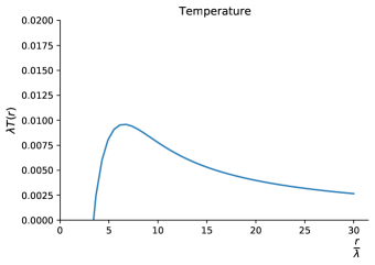
Figure 4: Temperature as a function of the radius, in units of $\lambda$.

This plot is very similar to Fig.(2) in the previous model with $\alpha=2$, with the absolute zero of the temperature corresponding to $r_{0}$ and no horizons present for $r_{H}<r_{0}$, as we would expect. The numerical results in the Planck units for this model are collected in Table 2.

$M_{0}$ :	$\left(2.5747013735\right.$	$\pm$	$\left.10^{-10}\right)$	$\lambda$
$r_{0(H)}$ :	$\left(3.38363\right.$	$\pm$	$\left.10^{-5}\right)$	$\lambda$
$r_{0(T)}$ :	$\left(3.3836342\right.$	$\pm$	$\left.10^{-7}\right)$	$\lambda$
$T_{m}$ :	$\left(9.6023522\right.$	$\pm$	$\left.10^{-7}\right)10^{-3}$	$1/\lambda$
$r_{m}$ :	$\left(6.5442890\right.$	$\pm$	$\left.10^{-7}\right)$	$\lambda$
$M_{m}$ :	$2.72$			$\lambda$

Table 2: The values of $r_{0(H)}$ and $M_{0}$ are calculated numerically from Fig.(3), while $r_{0(T)}$ is obtained from Fig.(4). Contrary to the results in Table 1, $r_{0(H)}$ and $r_{0(T)}$ are compatible. The value $M_{m}$ is obtained analytically.

Next we analyze the recoil velocity of the primordial black holes due to Hawking radiation. The number of emitted quanta from the peak temperature to $T=0$ is:

$$N_{q}\sim\frac{c^{2}(M_{m}-M_{0})}{T_{m}k_{B}}\approx 87\lambda^{2},$$ (20)

where the quantities in Table 2 are expressed in SI units. The recoil velocity the black hole due to the emission of these quanta is

$$v_{r} =\frac{M_{m}-M_{0}}{M_{0}\sqrt{N_{q}}}c=\frac{\sqrt{\left(M_{m}-M_{0}\right)T_{m}k_{B}}}{M_{0}}$$

$$\approx 1.04\times 10^{7}\frac{1}{\lambda}\text{ms}^{-1}.$$ (21)

Choosing $\lambda=1$ gives $v_{r}\approx 1.04\times 10^{4}$ km/s, then to match the results for the dark matter velocity as given in [63], we again need $\lambda\sim 10^{2}$.

We can draw the same conclusions as in the $\alpha=2$ model, namely primordial black holes with initial masses around the critical mass can be found near the peak of the temperature for every allowed value of $\lambda$ and they subsequently evaporate to a remnant with temperature $T=0$ and mass $M=M_{0}=5.60\times 10^{-8}$ $\lambda$ kg (a value larger than the Planck mass even for $L=\ell_{\text{P}}$). Also, primordial black holes with higher and lower masses are found far from the peak or as remnant near $T=0$, respectively.

.2 Model with $\alpha=3$

Another model results from taking $\alpha=3$ in the density function (3) and was proposed in [73]. The density was written as

$$\rho(r)=\epsilon_{0}e^{-\left(r/r_{*}\right)^{3}},$$ (22)

where

$$\epsilon_{0}=\frac{3c^{2}M}{4\pi r_{*}^{3}}\equiv\frac{M}{36\pi\lambda^{3}},$$ (23)

in which $M$ is a constant that indicates the total mass if this was a Schwarzschild black hole. In the above expression, we renamed the theory’s parameter $\epsilon_{0}$ so that we have the same structure as the other models. Also, we took $c=1$, consistently with our choice of units. The density then takes the following form:

$$\rho(r)=\frac{M}{36\pi\lambda^{3}}e^{-\left(r/(3\lambda)\right)^{3}}.$$ (24)

The Einstein equations give

$$\frac{1+f(r)+f^{\prime}(r)}{r^{2}}=8\pi T_{00}=\frac{2M}{9\lambda^{3}}e^{-\left(r/(3\lambda)\right)^{3}},$$ (25)

where, again, $g_{00}=f(r)=-g_{rr}^{-1}$ and $T^{0}_{0}=-\rho(r)$. The solution is:

$$f(r)=-1+\frac{2M}{r}\left[1-e^{-\left(r/(3\lambda)\right)^{3}}\right].$$ (26)

The event horizon is once again found by imposing $f(r)=0$. To obtain it numerically, we plot $f(r)$ and observe its intersections with the $r$ axis:

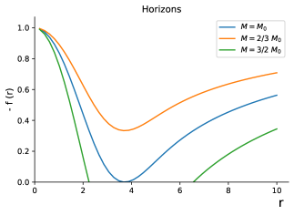
Figure 5: $-f(r)$ as a function of the radius, in units of $\lambda$ for $M=M_{0}$, $M=2/3$ $M_{0}$, $M=3/2$ $M_{0}$.

Horizons are formed only for $M\geqslant M_{0}$, and for $M=M_{0}$ they coincide. Next, the temperature can be calculated using $f(r)$ in Eq.(26):

$$T=-\left(\frac{1}{4\pi}\frac{\operatorname{d}\!{g}_{00}}{\operatorname{d}\!{r}}\right)_{r_{H}}.$$ (27)

Substituting the expression for $M(r_{H})$ easily obtainable from $f(r)=0$, we have:

$$T=\frac{1}{4\pi r_{H}}\left[1-\frac{3}{e^{\left(r_{H}/(3\lambda)\right)^{3}}-1}\left(\frac{r_{H}}{3\lambda}\right)^{3}\right].$$ (28)

The plot of the temperature, expressed in units of $\lambda$, is given in Fig.(6).

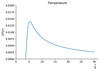
Figure 6: Temperature as a function of the radius, in units of $\lambda$.

The plot is analogous to the models studied previously (in figures 2 and 4), with the absolute zero of the temperature corresponds to $r_{0}$, and there is no horizon for $r_{H}<r_{0}$. The numerical results in the Planck units for this model are listed in Table 3 below.

$M_{0}$ :	$\left(2.1845877235\right.$	$\pm$	$\left.10^{-10}\right)$	$\lambda$
$r_{0(H)}$ :	$\left(3.71817\right.$	$\pm$	$\left.10^{-5}\right)$	$\lambda$
$r_{0(T)}$ :	$\left(3.7181714\right.$	$\pm$	$\left.10^{-7}\right)$	$\lambda$
$T_{m}$ :	$\left(1.4009975\right.$	$\pm$	$\left.10^{-7}\right)10^{-2}$	$1/\lambda$
$r_{m}$ :	$\left(5.2883955\right.$	$\pm$	$\left.10^{-7}\right)$	$\lambda$
$M_{m}$ :	$2.66$			$\lambda$

Table 3: The values of $r_{0(H)}$ and $M_{0}$ are calculated numerically from Fig.(5), while $r_{0(T)}$ is obtained from Fig.(6). Contrary to the results in Table 1, and similar to that in Table 2, $r_{0(H)}$ and $r_{0(T)}$ are compatible. The value $M_{m}$ is obtained analytically.

The recoil velocity is once again calculated from the number of emitted quanta from the peak temperature to $T=0$:

$$N_{q}\sim\frac{c^{2}(M_{m}-M_{0})}{T_{m}k_{B}}\approx 34\lambda^{2},$$ (29)

in SI units. The recoil velocity is then:

$$v_{r} =\frac{M_{m}-M_{0}}{M_{0}\sqrt{N_{q}}}c=\frac{\sqrt{\left(M_{m}-M_{0}\right)T_{m}k_{B}}}{M_{0}}$$

$$\approx 1.12\times 10^{7}\frac{1}{\lambda}\text{ms}^{-1}.$$ (30)

Choosing $\lambda=1$ gives $v_{r}\approx 1.12\times 10^{4}$ km/s, then to match the results in [63] we need $\lambda\sim 10^{2}$.

The model is again overall very similar to the previous two discussed.

.3 Model in Asymptotically Safe Gravity

Black hole properties arising from asymptotic safety have been analysed starting with the article by Bonanno and Reuter in [71]. In this treatment, we follow [72]. The radial function $f(r)$ under RG-improvement of a Schwarzschild black hole is:

$$f(r)=-1+\frac{4MGr^{2}}{2r^{3}+\omega G\left(2r+9GM\right)},$$ (31)

where $\omega$ is a parameter of the theory and $G$ is the usual Newton’s constant, which can be set to $1$ to use natural units. Imposing $f(r)=0$ gives the position of the event horizon, obtained numerically from the plot in Fig.(7), and the mass $M_{0}$:

$$M_{0}=2r\frac{r^{2}+\omega}{4r^{2}-9\omega}.$$ (32)

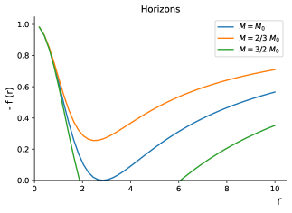
Figure 7: $-f(r)$ as a function of the radius, in natural units and for $\omega=1$, corresponding to the values $M=M_{0}$, $M=2/3$ $M_{0}$, $M=3/2$ $M_{0}$.

Horizons are formed only for $M\geqslant M_{0}$, and for $M=M_{0}$ they coincide. Next, the temperature can be calculated using $f(r)$ in (31):

$$T=-\frac{1}{4\pi}\left(\frac{\operatorname{d}\!{f}(r)}{\operatorname{d}\!{r}}\right)_{r_{H}},$$ (33)

giving the result:

$$T=\frac{Mr}{2\pi}\frac{r^{3}-\omega\left(r+9M\right)}{\left[r^{3}+\omega\left(r-\frac{9}{2}M\right)\right]^{2}},$$ (34)

where one could also substitute the expression for $M_{0}$ in (32). The plot of the temperature, expressed in natural units with $\omega=1$, is given in Fig.(8).

The plot is analogous to those of the non-commutativity models, with the absolute zero of the temperature corresponding to $r_{0}$, and the absence of horizons for $r_{H}<r_{0}$. The numerical results with $\omega=1$ are listed in Table 4 below.

$M_{0}$ :	$\left(2.2135416027\right.$	$\pm$	$\left.10^{-10}\right)$	$\omega m_{\text{p}}$
$r_{0(H)}$ :	$\left(2.8338\right.$	$\pm$	$\left.10^{-4}\right)$	$\omega\ell_{\text{p}}$
$r_{0(T)}$ :	$\left(2.8337594\right.$	$\pm$	$\left.10^{-7}\right)$	$\omega\ell_{\text{p}}$
$T_{m}$ :	$\left(1.0504229\right.$	$\pm$	$\left.10^{-7}\right)10^{-2}$	$T_{\text{p}}$
$r_{m}$ :	$\left(5.0020168\right.$	$\pm$	$\left.10^{-7}\right)$	$\omega\ell_{\text{p}}$
$M_{m}$ :	$2.86$			$\omega m_{\text{p}}$

Table 4: The values of $r_{0(H)}$ and $M_{0}$ are calculated numerically from figure 7, while $r_{0(T)}$ is obtained from figure 8. $r_{0(H)}$ and $r_{0(T)}$ are compatible. The value $M_{m}$ is obtained analytically.

Figure 8: Temperature as a function of the radius, in natural units with $\omega=1$.

The recoil velocity the black hole gets from the emission of quanta in the last part of its evolution then gives:

$$N_{q}\sim\frac{c^{2}(M_{m}-M_{0})}{T_{m}k_{B}}\approx 61,$$ (35)

when $\omega=1$. The recoil velocity is, under the same assumptions:

$$v_{r} =\frac{M_{m}-M_{0}}{M_{0}\sqrt{N_{q}}}c=\frac{\sqrt{\left(M_{m}-M_{0}\right)T_{m}k_{B}}}{M_{0}}$$

$$\approx 1.11\times 10^{4}\text{ }\frac{km}{s}.$$ (36)

Choosing $\omega=4000$ gives $v_{r}\approx 218$ km/s.

References

- [1] Vadim V. Zhytnikov, James M. Nester, “Can Galactic Observations Be Explained by a Relativistic Gravity Theory?”, Phys. Rev. Lett. 73 (1994) 2950, [arXiv:gr-qc/9410002].
- [2] Maxim Yu. Khlopov, “Primordial Black Holes”, Res. Astron. Astrophys. 10 (2010) 495, [arXiv:0801.0116 [astro-ph]].
- [3] Stephen Hawking, “Gravitationally Collapsed Objects of Very Low Mass”, Mon. Not. Roy. Astron. Soc. 152 (1971) 75.
- [4] Bernard J. Carr, Stephen Hawking, “Black Holes in the Early Universe”, Mon. Not. Roy. Astron. Soc. 168 (1974) 399.
- [5] David J. Gross, Malcolm J. Perry, Laurence G. Yaffe, “Instability of Flat Space at Finite Temperature”, Phys. Rev. D 25 (1982) 330.
- [6] Joseph I. Kapusta, “Nucleation Rate for Black Holes”, Phys. Rev. D 30 (1984) 831.
- [7] Rostislav V. Konoplich, Sergei G. Rubin, Alexander S. Sakharov, Maxim Yu. Khlopov, “Formation of Black Holes in First-Order Phase Transitions as a Cosmological Test of Symmetry-Breaking Mechanisms”, Phys. Atom. Nucl. 62 (1999) 1593, Yad. Fiz. 62 (1999) 1705.
- [8] Rostislav V. Konoplich, Sergei G. Rubin, Alexander S. Sakharov, Maxim Yu. Khlopov, “First Order Phase Transitions as a Source of Black Holes in the Early Universe”, Grav. Cosmol. 2 (1999) S1, [arXiv:hep-ph/9912422].
- [9] Joseph I. Kapusta, Todd Springer, “Cosmological Black Hole Formation due to QCD and Electroweak Phase Transitions”, [arXiv:0706.1111 [astro-ph]].
- [10] David Polarski and Alexei A. Starobinsky, “ Isocurvature Perturbations in Multiple Inflationary Models”, Phys. Rev. D 50 (1994) 6123 , [arXiv:astro-ph/9404061].
- [11] P. Ivanov, Pavel Naselsky, Igor Novikov, “Inflation and Primordial Black Holes as Dark Matter”, Phys. Rev. D 50 (1994) 7173.
- [12] Pisin Chen, “Inflation Induced Planck-Size Black Hole Remnants As Dark Matter”, New Astron. Rev. 49 (2005) 233, [arXiv:astro-ph/0406514].
- [13] Guillermo Ballesteros, Marco Taoso, “Primordial Black Hole Dark Matter From Single Field Inflation”, Phys. Rev. D 97 (2018) 023501, [arXiv:1709.05565 [hep-ph]].
- [14] Shi Pi, Ying-li Zhang, Qing-Guo Huang, Misao Sasaki, “Scalaron From -Gravity as a Heavy Field”, JCAP 05 (2018) 042, [arXiv:1712.09896 [astro-ph.CO]].
- [15] Ioannis Dalianis, George Tringas, “PBH Remnants as Dark Matter Produced in Thermal, Matter and Runaway-Quintessence Post-Inflationary Scenarios”, Phys. Rev. D 100 (2019) 083512, [arXiv:1905.01741 [astro-ph.CO]].
- [16] Nilanjandev Bhaumik, Rajeev Kumar Jain, “Primordial Black Holes Dark Matter From Inflection Point Models of Inflation and the Effects of Reheating”, JCAP 01 (2020) 037, [arXiv:1907.04125 [astro-ph.CO]].
- [17] Richa Arya, “Formation of Primordial Black Holes from Warm Inflation”, JCAP 09 (2020) 042, [arXiv:1910.05238 [astro-ph.CO]].
- [18] Rong-Gen Cai, Zong-Kuan Guo, Jing Liu, Lang Liu, Xing-Yu Yang, “Primordial Black Holes and Gravitational Waves From Parametric Amplification of Curvature Perturbations”, JCAP 06 (2020) 013, [arXiv:1912.10437 [astro-ph.CO]].
- [19] Matteo Braglia, Dhiraj Kumar Hazra, Fabio Finelli, George F. Smoot, L. Sriramkumar, Alexei A. Starobinsky, “ Generating PBHs and small-scale GWs in two-field models of inflation”, JCAP 2008 (2020) 001, [arXiv:2005.02895[astro-ph.CO].
- [20] Keisuke Inomata, Evan McDonough, Wayne Hu, “Primordial Black Holes Arise When The Inflaton Falls”, [arXiv:2104.03972 [astro-ph.CO]].
- [21] Pisin Chen, Ronald J. Adler, “Black Hole Remnants and Dark Matter”, Nucl. Phys. Proc. Suppl. 124 (2003) 103, [arXiv:gr-qc/0205106].
- [22] Bernard J. Carr, “Primordial Black Holes: Do They Exist and Are They Useful?”, [arXiv:astro-ph/0511743].
- [23] Bernard Carr, Florian Kuhnel, “Primordial Black Holes as Dark Matter: Recent Developments”, Ann. Rev. Nucl. Part. Sci. 70 (2020) 355, [arXiv:2006.02838 [astro-ph.CO]].
- [24] Anne M. Green, Bradley J. Kavanagh, “Primordial Black Holes as a Dark Matter Candidate”, J. Phys. G 48 (2021) 4, 043001, [arXiv:2007.10722 [astro-ph.CO]].
- [25] Chen Yuan, Zu-Cheng Chen, Qing-Guo Huang, “Probing Primordial-Black-Hole Dark Matter with Scalar Induced Gravitational Waves”, Phys. Rev. D 100 (2019) 081301, [arXiv:1906.11549 [astro-ph.CO]].
- [26] Bernard Carr, Florian Kuhnel, Luca Visinelli, “Black Holes and WIMPs: All or Nothing or Something Else”, [arXiv:2011.01930 [astro-ph.CO]].
- [27] Chen Yuan, Qing-Guo Huang, “A Topic Review on Probing Primordial Black Hole Dark Matter With Scalar Induced Gravitational Waves”, [arXiv:2103.04739 [astro-ph.GA]].
- [28] Bernard Carr, Kazunori Kohri, Yuuiti Sendouda, Jun’ichi Yokoyama, “Constraints on Primordial Black Holes”, Phys. Rev. Lett. 125 (2020) 101101, [arXiv:2002.12778 [astro-ph.CO]].
- [29] Ranjan Laha, “Primordial Black Holes as a Dark Matter Candidate Are Severely Constrained by the Galactic Center 511 Kev Gamma-Ray Line”, Phys. Rev. Lett. 123 (2019) 251101, [arXiv:1906.09994 [astro-ph.HE]].
- [30] Basudeb Dasgupta, Ranjan Laha, Anupam Ray, “Neutrino and Positron Constraints on Spinning Primordial Black Hole Dark Matter”, Phys. Rev. Lett. 125 (2020) 101101, [arXiv:1912.01014 [hep-ph]].
- [31] Ranjan Laha, Julian B. Muñoz, Tracy R. Slatyer, “Integral Constraints on Primordial Black Holes and Particle Dark Matter”, Phys. Rev. D 101 (2020) 123514, [arXiv:2004.00627 [astro-ph.CO]].
- [32] Rong-Gen Cai, Yu-Chen Ding, Xing-Yu Yang, Yu-Feng Zhou, “Constraints on a Mixed Model of Dark Matter Particles and Primordial Black Holes From the Galactic 511 Kev Line”, JCAP 03 (2021) 057, [arXiv:2007.11804 [astro-ph.CO]].
- [33] Irina Dymnikova, Maxim Khlopov, “Regular Black Hole Remnants and Graviatoms With de Sitter Interior as Heavy Dark Matter Candidates Probing Inhomogeneity of Early Universe”, Int. J. Mod. Phys. D 24 (2015) 13, 1545002,[arXiv:1510.01351 [gr-qc]].
- [34] Sebastien Clesse, Juan GarcÃa-Bellido, Stefano Orani, “Detecting the Stochastic Gravitational Wave Background from Primordial Black Hole Formation”, [arXiv:1812.11011 [astro-ph.CO]].
- [35] Yi-Fu Cai, Chao Chen, Xi Tong, Dong-Gang Wang, Sheng-Feng Yan, “When Primordial Black Holes from Sound Speed Resonance Meet a Stochastic Background of Gravitational Waves”, Phys. Rev. D 100 (2019) 043518, [arXiv:1902.08187 [astro-ph.CO]].
- [36] Alexander Kusenko, Misao Sasaki, Sunao Sugiyama, Masahiro Takada, Volodymyr Takhistov, Edoardo Vitagliano, “Exploring Primordial Black Holes from the Multiverse with Optical Telescopes”, Phys. Rev. Lett. 125 (2020) 181304, [arXiv:2001.09160 [astro-ph.CO]].
- [37] Keisuke Inomata, Masahiro Kawasaki, Kyohei Mukaida, Takahiro Terada, Tsutomu T. Yanagida, “Gravitational Wave Production right after a Primordial Black Hole Evaporation”, Phys. Rev. D 101 (2020) 123533, [arXiv:2003.10455 [astro-ph.CO]].
- [38] Anupam Ray, Ranjan Laha, Julian B. Muñoz, Regina Caputo, “Closing the Gap: Near Future Mev Telescopes Can Discover Asteroid-Mass Primordial Black Hole Dark Matter”, [arXiv:2102.06714 [astro-ph.CO]].
- [39] Rampei Kimura, Teruaki Suyama, Masahide Yamaguchi, Ying-li Zhang, “Reconstruction of Primordial Power Spectrum of curvature perturbation from the merger rate of Primordial Black Hole Binaries”, JCAP 04 (2021) 031, [arXiv:2102.05280 [astro-ph.CO]].
- [40] Rong-gen Cai, Shi Pi, Misao Sasaki, “Gravitational Waves Induced by non-Gaussian Scalar Perturbations”, Phys. Rev. Lett. 122 (2019) 201101, [arXiv:1810.11000 [astro-ph.CO]].
- [41] Sai Wang, Dong-Mei Xia, Xukun Zhang, Shun Zhou, Zhe Chang, “Constraining Primordial Black Holes as Dark Matter at Juno”, Phys. Rev. D 103 (2021) 043010, [arXiv:2010.16053 [hep-ph]].
- [42] Mark P. Hertzberg, Sami Nurmi, Enrico D. Schiappacasse, Tsutomu T. Yanagida, “Shining Primordial Black Holes”, Phys. Rev. D 103 (2021) 063025, [arXiv:2011.05922 [hep-ph]].
- [43] Ville Vaskonen, Hardi Veermäe, “Did NANOGrav See a Signal From Primordial Black Hole Formation?”, Phys. Rev. Lett. 126 (2021) 051303, [arXiv:2009.07832 [astro-ph.CO]].
- [44] Valerio De Luca, Gabriele Franciolini, Antonio Riotto, “NANOGrav Data Hints at Primordial Black Holes as Dark Matter”, Phys. Rev. Lett. 126 (2021) 4, 041303, [arXiv:2009.08268 [astro-ph.CO]].
- [45] Guillem Domènech, Shi Pi, “NANOGrav Hints on Planet-Mass Primordial Black Holes”, [arXiv:2010.03976 [astro-ph.CO]].
- [46] Pisin Chen, Yen Chin Ong, Dong-han Yeom, “Black Hole Remnants and the Information Loss Paradox”, Phys. Rept. 603 (2015) 1, [arXiv:1412.8366 [gr-qc]].
- [47] Samuel Kováčik, “Hawking-Radiation Recoil of Microscopic Black Holes”, [arXiv:2102.06517 [gr-qc]].
- [48] Valeri Frolov, Dejan Stojkovic, “Black Hole Radiation in the Brane World and Recoil Effect”, Phys. Rev. D 66 (2002) 084002, [arXiv:hep-th/0206046].
- [49] Valeri Frolov, Dejan Stojkovic, “Black Hole as a Point Radiator and Recoil Effect on the Brane World”, Phys. Rev. Lett. 89 (2002) 151302, [arXiv:hep-th/0208102].
- [50] Don N. Page, “Is Black-Hole Evaporation Predictable?”, Phys. Rev. Lett. 44 (1980) 301.
- [51] Yasunori Nomura, Jaime Varela, Sean J. Weinberg, “Black Holes, Information, and Hilbert Space for Quantum Gravity”, Phys. Rev. D 87 (2013) 084050, [arXiv:1210.6348 [hep-th]].
- [52] Ronald J. Adler, Pisin Chen, David I. Santiago, “The Generalized Uncertainty Principle and Black Hole Remnants”, Gen. Rel. Grav. 33 (2001) 2101, [arXiv:gr-qc/0106080].
- [53] Ronald J. Adler, “Six Easy Roads to the Planck Scale”, Am. J. Phys. 78 (2010) 925, [arXiv:1001.1205 [gr-qc]].
- [54] Piero Nicolini, “Noncommutative Black Holes, The Final Appeal to Quantum Gravity: A Review”, Int. J. of Mod. Phys A 24 (2009) 1229, [arXiv:0807.1939 [hep-th]]
- [55] Anna Pachołl, “Short Review on Noncommutative Spacetimes”, J. Phys. Conf. Ser. 442 (2013) 012039.
- [56] Michael R. Douglas, Nikita A. Nekrasov, “Noncommutative Field Theory”, Rev. Mod. Phys. 73 (2001) 977, [arXiv:hep-th/0106048].
- [57] Sabine Hossenfelder, “Minimal Length Scale Scenarios for Quantum Gravity”, Living Rev. Rel. 16 (2013) 2, [arXiv:1203.6191 [gr-qc]].
- [58] Nathan Seiberg, Edward Witten, “String Theory and Noncommutative Geometry”, JHEP 9909 (1999) 032, [arXiv:hep-th/9908142].
- [59] Robert Brandenberger, “String Theory, Space-Time Non-Commutativity and Structure Formation”, Prog. Theor. Phys. Suppl. 171 (2007) 121, [arXiv:hep-th/0703173].
- [60] Piero Nicolini, Anais Smailagic, Euro Spallucci, “Noncommutative Geometry Inspired Schwarzschild Black Hole”, Phys. Lett. B 632 (2006) 547, [arXiv:gr-qc/0510112].
- [61] Rui Vilela-Mendes, “Space-time: Commutative or Noncommutative ?”, Phys. Rev. D 99 (2019) 123006, [arXiv:1901.01613 [hep-th]].
- [62] Samuel Kováčik, “ Inspired Black Holes”, [arXiv:1504.04460 [gr-qc]].
- [63] Laura Baudis, Stefano Profumo, “Dark Matter”, in Review of Particle Physics by Particle Data Group, Prog. Theo. and Exp. Phys. 2020 (2020) 083C01, p.476.
- [64] Jorge Ernesto Horvath, Paulo Sergio Custódio , “Some Results on the Evolution of Primordial Black Holes”, Braz. J. Phys. 35 no.4b (2005) 210
- [65] Jared R. Rice, Bing Zhang, “Cosmological Evolution of Primordial Black Holes”, JHEAp 13-14 (2017) 22, [arXiv:1702.08069 [astro-ph.HE]].
- [66] Finnian Gray, Sebastian Schuster, Alexander Van-Brunt, Matt Visser, “The Hawking Cascade From a Black Hole Is Extremely Sparse”, Class. Quant. Grav. 33 (2016) 11, 115003, [arXiv:1506.03975 [gr-qc]].
- [67] Benjamin V. Lehmann, Stefano Profumo, “Black Hole Remnants Are Not Too Fast to Be Dark Matter”, [arXiv:2105.01627 [gr-qc]].
- [68] S. Ali Alavi, “Reissner-Nordström Black Hole In Noncommutative Spaces”, Acta Phys. Polon. B 40 (2009) 2679, [arXiv:0909.1688 [gr-qc]].
- [69] Leonardo Modesto, Piero Nicolini, “Charged Rotating Noncommutative Black Holes”, Phys. Rev. D 82 (2010) 104035, [ arXiv:1005.5605 [gr-qc]].
- [70] Biplab Paik, “Charge and/or Spin Limits for Black Holes at a Non-Commutative Scale”, Pramana 89 (2017) 26.
- [71] Alfio Bonanno, Martin Reuter, “Spacetime Structure of an Evaporating Black Hole in Quantum Gravity”, Phys. Rev. D 73 (2006) 083005, [arXiv:hep-th/0602159].
- [72] Benjamin Koch, Frank Saueressig, “Black holes within Asymptotic Safety”, Int. J. Mod. Phys. A 29 (2014) 8, 1430011, [arXiv:1401.4452 [hep-th]].
- [73] Irina Dymnikova, “Vacuum Nonsingular Black Hole”, Gen. Relativ. Gravit. 24 (1992) 235.