The level repulsion exponent of localized chaotic eigenstates as a function of the classical transport time scales in the stadium billiard

Abstract

We study the aspects of quantum localization in the stadium billiard, which is a classically chaotic ergodic system, but in the regime of slightly distorted circle billiard the diffusion in the momentum space is very slow. In quantum systems with discrete energy spectrum the Heisenberg time $t_{H}=2\pi\hbar/\Delta E$, where $\Delta E$ is the mean level spacing (inverse energy level density), is an important time scale. The classical transport time scale $t_{T}$ (diffusion time) in relation to the Heisenberg time scale $t_{H}$ (their ratio is the parameter $\alpha=t_{H}/t_{T}$) determines the degree of localization of the chaotic eigenstates, whose measure $A$ is based on the information entropy. The localization of chaotic eigenstates is reflected also in the fractional power-law repulsion between the nearest energy levels in the sense that the probability density (level spacing distribution) to find successive levels on a distance $S$ goes like $\propto S^{\beta}$ for small $S$, where $0\leq\beta\leq 1$, and $\beta=1$ corresponds to completely extended states. We show that the level repulsion exponent $\beta$ is a unique rational function of $\alpha$, and $A$ is a unique rational function of $\alpha$. $\beta$ goes from $0$ to $1$ when $\alpha$ goes from $0$ to $\infty$. Also, $\beta$ is a linear function of $A$, which is similar as in the quantum kicked rotator, but different from a mixed type billiard.

I Introduction

In quantum chaos we study phenomena in the quantum domain, or in other wave systems described also by the wave equations different from the Schrödinger equation, which correspond to the classical chaos in the semiclassical limit (short wavelength approximation) Stöckmann (1999); Haake (2001). The quantum localization of classical chaotic diffusion in the time-dependent domain is one of the most important fundamental phenomena in quantum chaos, discovered and studied first in the quantum kicked rotator Casati et al. (1979); Chirikov et al. (1981, 1988); Izrailev (1990) by Chirikov, Casati, Izrailev, Shepelyansky, Guarneri and many others. An excellent extensive account and review has been given by Izrailev Izrailev (1988, 1989, 1990). This type of phenomena is generic in chaotic Floquet (time-periodic) Hamilton systems.

In the time-independent domain the quantum localization is manifested in the localized chaotic eigenstates. In the case of the quantum kicked rotator, for example, one sees the exponentially localized eigenstates in the dimensionless space of the angular momentum quantum number. For an extensive review see Izrailev (1990). This phenomenon is closely related to the Anderson localization in one dimensional disordered lattices as shown for the first time by Fishman, Grempel and Prange Fishman et al. (1982), and later discussed and studied by many others Stöckmann (1999); Haake (2001).

The quantum localization in billiards has been reviewed by Prosen in reference Prosen (2000). Here we have to look at the localization properties of the localized chaotic eigenstates in the quantum phase space, which means study of the Wigner functions (which are real valued but not positive definite), or better, the Husimi functions, which are real and positive definite, and can be treated as a quasi-probability density. In the semiclassical limit we are interested in the quantum-classical correspondence of these structures in the phase spaces.

Recently, we Batistić and Robnik (2013a) have studied the localization of chaotic eigenstates in the mixed-type billiard Robnik (1983, 1984), after the separation of the chaotic and regular eigenstates based on such quantum-classical correspondence Batistić and Robnik (2013b). We have introduced two localization measures, one based on the information entropy denoted by $A$ and used in this paper, and the other one $C$ based on the correlations. We have shown that $A$ and $C$ are linearly related and thus equivalent.

In this paper we study localization properties of eigenstates in the stadium billiard of Bunimovich Bunimovich (1979), which is a chaotic ergodic system. Studies of the slow diffusive regime in this system and the related quantum localization were initiated in Ref. Borgonovi et al. (1996), while the detailed aspects of classical diffusion have been investigated in our recent paper Č. Lozej and Robnik (2018).

Another fundamental phenomenon in quantum chaos in the time-independent domain is the statistics of the fluctuations in the energy spectra. In analogy with the time-periodic systems we find functional relationship between the localization measure $A$ and the spectral (energy) level repulsion exponent $\beta$, to be precisely defined below. $A$ and $\beta$ are unique functions of the parameter $\alpha=t_{H}/t_{T}$, which by definition is the ratio of two most important time scales in the system, namely the Heisenberg time $t_{H}=2\pi\hbar/\Delta E$, where $\Delta E$ is the mean energy level spacing, and the classical transport (diffusion) time scale $t_{T}$. These findings are the main result of this work.

The statistical properties of energy spectra of quantum systems are universal Stöckmann (1999); Haake (2001); Mehta (1991); Guhr et al. (1998); Robnik (1998). In the sufficiently deep semiclassical limit (when $\alpha$ is large enough, $\alpha\gg 1$, which can always been achieved by sufficiently small effective $\hbar$) and in general mixed type systems, they are determined solely by the type of classical motion, which can be either regular or chaotic Percival (1973); Berry and Robnik (1984); Robnik (1998); Batistić and Robnik (2010, 2013a, 2013b). The level statistics is Poissonian if the underlying classical invariant component is regular, whilst for chaotic extended states the Random Matrix Theory (RMT) applies Mehta (1991), specifically the Gaussian Orthogonal Ensemble statistics (GOE) in case of an antiunitary symmetry. This is the Bohigas-Giannoni-Schmit conjecture Casati et al. (1980); Bohigas et al. (1984), which has been proven only recently Sieber and Richter (2001); Müller et al. (2004); Heusler et al. (2004); Müller et al. (2005, 2009) using the semiclassical methods and the periodic orbit theory developed around 1970 by Gutzwiller (Gutzwiller (1980) and the references therein), an approach initiated by Berry Berry (1985), well reviewed in Stöckmann (1999); Haake (2001).

The classification regular-chaotic can be done by analyzing the structure of eigenstates in the quantum phase space, based on the Wigner functions, or Husimi functions Batistić and Robnik (2013b). Of course, in the stadium billiard all eigenstates are of the chaotic type, but can be strongly localized if $\alpha$ is small enough, $\alpha\ll 1$.

The most important statistical measure is the level spacing distribution $P(S)$, assuming spectral unfolding such that $\left<S\right>=1$. For integrable systems and regular levels of mixed type systems $P(S)=\exp\left(-S\right)$, whilst for extended chaotic systems it is well approximated by the Wigner distribution $P(S)=\frac{\pi S}{2}\exp\left(-\frac{\pi}{4}\,S^{2}\right)$. The distributions differ significantly in a small $S$ regime, where there is no level repulsion in a regular system and a linear level repulsion, $P(S)\propto S$, in a chaotic system. Localized chaotic states exhibit the fractional power-law level repulsion $P(S)\propto S^{\beta}$, as clearly demonstrated recently by Batistić and Robnik Batistić and Robnik (2010, 2013a, 2013b).

The localization is a pure quantum effect which appears if the Heisenberg time $t_{H}$, which is the time scale on which the quantum evolution follows the classical one, is smaller than the relevant classical transport time $t_{T}$ (diffusion or ergodic time). Up to the Heisenberg time the quantum system behaves as if the evolution operator had a continuous spectrum, but at times longer than Heisenberg time the discrete spectrum of the evolution operator becomes resolved, and the interference effects set in, resulting in a destructive interference causing the quantum localization. Thus the parameter $\alpha=t_{H}/t_{T}$ plays a key role. The ergodic time may be very long, especially if the chaotic region has a complicated, but typical KAM structure, due to the presence of the partial barriers in the form of barely destroyed irrational tori, called cantori, which allow for a very slow transport only. However, in this paper we study the stadium, which is ergodic, so no KAM structures are present, although cantori can be and in fact are present.

The weak ($\beta<1$) level repulsion of localized states is empirically observed, but the whole distribution $P(S)$ is globally theoretically not known. Several different distributions which would extrapolate the small $S$ behaviour were proposed. The most popular are the Izrailev distribution Izrailev (1988, 1989, 1990) and the Brody distribution Brody (1973); Brody et al. (1981). The Brody distribution is a simple generalization of the Wigner distribution. Explicitly, the Brody distribution is

$$P_{B}(S)=cS^{\beta}\exp\left(-dS^{\beta+1}\right),\;\;\;$$ (1)

where

$$c=(\beta+1)d,\;\;\;d=\left(\Gamma\left(\frac{\beta+2}{\beta+1}\right)\right)^{\beta+1}$$ (2)

with $\Gamma(x)$ being the Gamma function. It interpolates the exponential and Wigner distribution as $\beta$ goes from $0$ to $1$. The Izrailev distribution is a bit more complicated but has the feature of being a better approximation for the GOE distribution at $\beta=1$. One important theoretical plausibility argument by Izrailev in support of such intermediate level spacing distributions is that the joint level distribution of Dyson circular ensembles can be extended to noninteger values of the exponent $\beta$ Izrailev (1990). However, recent numerical results show that Brody distribution is slightly better in describing real data Batistić and Robnik (2010, 2013a); Manos and Robnik (2013); Batistić et al. (2013), and is simpler, which is the reason why we prefer and use it.

The open question is how does the level repulsion parameter $\beta$ depend on the localization. This question was raised for the first time by Izrailev Izrailev (1988, 1989, 1990), where he numerically studied the quantum kicked rotator, which is a 1D time-periodic system. His result showed that the parameter $\beta$, which was obtained using the Izrailev distribution, is functionally related to the localization measure defined as the information entropy of the eigenstates in the angular momentum representation. His results were recently confirmed and extended, with the much greater numerical accuracy and statistical significance Manos and Robnik (2013); Batistić et al. (2013). Moreover, in Ref. Batistić and Robnik (2013a) it has been demonstrated that $\beta$ is a unique function of $A$ in the billiard with the mixed phase space Robnik (1983, 1984).

In this paper we show that there is indeed a functional relation between the level repulsion parameter $\beta$ and the localization measure $A$ also in the stadium billiard, in analogy with the quantum kicked rotator and the above mentioned billiard, but the functional form is different. We also show that $\beta$ is a unique function of $\alpha$.

II The billiard systems and Poincaré-Husimi functions

The stadium billiard Bunimovich (1979) is defined as two semicircles of radius 1 connected by two parallel straight lines of lentgh $\varepsilon$, as shown in Fig. 1.

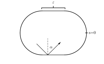
Figure 1: The geometry and notation of the stadium billiard of Bunimovich.

For a 2D billiard the most natural coordinates in the phase space $(s,p)$ are the arclength $s$ round the billiard boundary, $s\in[0,{\cal L}]$, where ${\cal L}$ is the circumference, and the sine of the reflection angle, which is the component of the unit velocity vector tangent to the boundary at the collision point, equal to $p=\sin\alpha$, which is the canonically conjugate momentum to $s$. These are the Poincaré-Birkhoff coordinates. The bounce map $(s_{1},p_{1})\rightarrow(s_{2},p_{2})$ is area preserving, and the phase portrait does not depend on the speed (or energy) of the particle. Quantum mechanically we have to solve the stationary Schrödinger equation, which in a billiard is just the Helmholtz equation $\Delta\psi+k^{2}\psi=0$ with the Dirichlet boundary conditions $\psi|_{\partial{\cal B}}=0$. The energy is $E=k^{2}$. The important quantity is the boundary function

$$u(s)={\bf n}\cdot\nabla_{{\bf r}}\psi\left({\bf r}(s)\right),$$ (3)

which is the normal derivative of the wavefunction $\psi$ at the point $s$ (${\bf n}$ is the unit normal vector). It satisfies the integral equation

$$u(s)=-2\oint dt\;u(t)\;{\bf n}\cdot\nabla_{{\bf r}}G({\bf r},{\bf r}(t)),$$ (4)

where $G({\bf r},{\bf r^{\prime}})=-\frac{i}{4}H_{0}^{(1)}(k|{\bf r}-{\bf r^{\prime}}|)$ is the Green function in terms of the Hankel function $H_{0}(x)$. It is important to realize that boundary function $u(s)$ contains complete information about the wavefunction at any point ${\bf r}$ inside the billiard by the equation

$$\psi_{m}({\bf r})=-\oint dt\;u_{m}(t)\;G\left({\bf r},{\bf r}(t)\right).$$ (5)

Here $m$ is just the index (sequential quantum number) of the $m$-th eigenstate. Now we go over to the quantum phase space. We can calculate the Wigner functions Wigner (1932) based on $\psi_{m}({\bf r})$. However, in billiards it is advantageous to calculate the Poincaré - Husimi functions. The Husimi functions Husimi (1940) are generally just Gaussian smoothed Wigner functions. Such smoothing makes them positive definite, so that we can treat them somehow as quasi-probability densities in the quantum phase space, and at the same time we eliminate the small oscillations of the Wigner functions around the zero level, which do not carry any significant physical contents, but just obscure the picture. Thus, following Tualle and Voros Tualle and Voros (1995) and Bäcker et al Bäcker et al. (2004), we introduce Batistić and Robnik (2013a, b). the properly ${\cal L}$-periodized coherent states centered at $(q,p)$, as follows

$$c_{(q,p),k}(s) = \sum_{m\in{\bf Z}}\exp\{i\,k\,p\,(s-q+m{\cal L})\}\times$$

$$\exp \left(-\frac{k}{2}(s-q+m{\cal L})^{2}\right).$$

The Poincaré - Husimi function is then defined as the absolute square of the projection of the boundary function $u(s)$ onto the coherent state, namely

$$H_{m}(q,p)=\left|\int_{\partial{\cal B}}c_{(q,p),k_{m}}(s)\;u_{m}(s)\;ds\right|^{2}.$$ (7)

The entropy localization measure denoted by $A$ is defined as

$$A=\frac{\exp\left<I\right>}{N_{c}},$$ (8)

where

$$I=-\int dq\,dp\,H(q,p)\ln\left((2\pi\hbar)^{f}H(q,p)\right)$$ (9)

is the information entropy. Here $f$ is the number of degrees of freedom (for 2D billiards $f=2$) and $N_{c}$ is a number of cells on the classical chaotic domain, $N_{c}=\Omega_{c}/(2\pi\hbar)^{f}$, where $\Omega_{c}$ is the classical phase space volume of the classical chaotic component. The mean $\left<I\right>$ is obtained by averaging $I$ over a sufficiently large number of consecutive chaotic eigenstates. In the case of uniform distribution (extended eigenstates) $H=1/\Omega_{C}={\rm const.}$ the localization measure is $A=1$, while in the case of the strongest localization $I=0$, and $A=1/N_{C}\approx 0$. The Poincaré - Husimi function $H(q,p)$ (7) (normalized) was calculated on the grid points $(i,j)$ in the phase space $(s,p)$. We express the localization measure in terms of the discretized Husimi function. In our numerical calculations we have put $2\pi\hbar=1$, and thus $H_{ij}=1/N_{C}$ in case of extendedness, while for maximal localization $H_{ij}=1$ at just one point, and zero elsewhere.

To get a good estimate of $\beta$ we need many more levels (eigenstates) than in calculating $A$. The parameter $\beta$ was computed for 40 diffrent values of the parameter $\epsilon$: $\epsilon_{j}=0.01+0.0025\,j$ where $j\in[0,1..39]$ and on 12 intervals in $k$ space: $(k_{i},k_{i+1})$ where $k_{i}=500+290\,i$ and $i\in[0,1..11]$. This is $40\times 12=480$ values of $\beta$ altogether. More than $4\times 10^{6}$ energy levels were computed for each $\epsilon$. The size of the intervals in $k$ was chosen to be maximal and such that the Brody distribution gives a good fit to the level spacing distributions of the levels in the intervals.

For each $\beta(\epsilon_{j},(k_{i},k_{i+1}))$ an associated localization measure $A$ was computed on a sample of 1000 consecutive levels around $\bar{k}_{i}=(k_{i}+k_{i+1})/2$, which is a mean value of $k$ on the interval $(k_{i},k_{i+1})$.

The almost linear dependence of $\beta$ on $A$ is shown in Fig. 2.

Figure 2: The level repulsion exponent $\beta$ as a function of the entropy localization measure $A$ for variety of stadia of different shapes $\varepsilon$ and energies $E=k^{2}$.

This is very similar to the case of the quantum kicked rotator Izrailev (1990); Manos and Robnik (2013); Batistić et al. (2013). In both cases the scattering of points around the mean linear behaviour is significant, and probably it is related to the fact that the localization measure of eigenstates has some distribution, as observed and discussed in Ref. Manos and Robnik (2015). There is a great lack in theoretical understanding of the physical origin of this phenomenon, even in the case of (the long standing research on) the quantum kicked rotator, except for the intuitive idea, that energy spectral properties should be only a function of the degree of localization, because the localization gradually decouples the energy eigenstates and levels, switching the linear level repulsion $\beta=1$ (extendedness) to a power law level repulsion with exponent $\beta<1$ (localization). The full physical explanation is open for the future.

III The role of the classical transport time scales

As explained in the introduction the role of classical transport time scale $t_{T}$ is importnat in the semiclassical limit (short wavelength approximation), in relation to the Heisenberg time scale $t_{H}$. We define the parameter $\alpha=t_{H}/t_{T}$, which controls the quantum localization phenomenon. Usually, as in Ref. Batistić and Robnik (2013b), $t_{T}$ is definesd as the time at which an ensemble of initial conditions in the momentum space with initial zero variance of its Dirac delta distribution reaches a certain fraction of the asymptotic value. In the stadium billiard for small $\varepsilon$ we have a diffusive regime and thus $t_{T}$ can be defined as the diffusion time extracted from the exponential approach of the momentum variance to the asymptotic value, as has been recently carefully studied in Ref. Č. Lozej and Robnik (2018).

For the sake of completeness we derive here the formula for $\alpha$ in billiards, following the presentation in Ref. Batistić and Robnik (2013b). In billiards the transport time can be also defined in terms of the number of collisions (bounces, or iterations of the bounce map), the discrete number $N_{T}$.

Let us consider the Heisenberg time and the classical transport time for a chaotic billiard. According to the leading order of the Weyl formula, which is in fact just the simple Thomas-Fermi rule, we have for the number of levels $N(E)$ below and up to the energy $E$ of a Hamiltonian $H({\bf q},{\bf p})$

$$N(E)=\frac{1}{(2\pi\hbar)^{2}}\int_{H({\bf q},{\bf p})\leq E}d^{2}{\bf q}\;d^{2}{\bf p}.$$ (10)

Since $H={\bf p}^{2}/(2m)$, with constant zero potential energy inside the billiard ${\cal B}$, where $m$ is the mass of the billiard point particle, and $H$ is infinite on the boundary $\partial{\cal B}$, we get at once

$$N(E)=\frac{2\pi{\cal A}mE}{(2\pi\hbar)^{2}}.$$ (11)

Here ${\cal A}$ is the area of the billiard ${\cal B}$. The density of levels is $\rho(E)=1/(\Delta E)=dN(E)/dE={\cal A}m/(2\pi\hbar^{2})$ and thus the Heisenberg time is

$$t_{H}=2\pi\hbar\rho(E)=\frac{{\cal A}m}{\hbar}.$$ (12)

The classical transport time is denoted by $t_{T}$, and in units of the number of collisions $N_{T}$ can be written as

$$t_{T}=\frac{\bar{l}N_{T}}{v}=\frac{\bar{l}N_{T}}{\sqrt{2E/m}},$$ (13)

where $\bar{l}$ is the mean free path of the billiard particle and $v=\sqrt{2E/m}$ is its speed at the energy $E$. Thus for the ratio $\alpha=t_{H}/t_{T}$ we get

$$\alpha=\frac{t_{H}}{t_{T}}=\frac{{\cal A}k}{N_{T}\bar{l}}$$ (14)

where $k=\sqrt{2mE/\hbar^{2}}$. Taking into account that $\bar{l}\approx\pi{\cal A}/{\cal L}$ (this is so-called Santalo’s formula, see e.g. Santaló and Kac (2004)), we have

$$\alpha=\frac{t_{H}}{t_{T}}=\frac{{\cal L}k}{\pi N_{T}},$$ (15)

where ${\cal L}$ is the length of the perimeter $\partial{\cal B}$. This is a general formula valid for any chaotic billiard. In the case of the stadium billiard with small $\varepsilon$ we have ${\cal L}\approx 2\pi$ and we arrive at the final estimate

$$\alpha=\frac{2k}{N_{T}}.$$ (16)

Thus the condition for the occurrence of dynamical localization $\alpha\leq 1$ is now expressed in the inequality

$$k\leq\frac{N_{T}}{2}.$$ (17)

Of course, the definition of the classical transport time is rather arbitrary. One definition is in terms of the diffusion time which appears in the exponential approach of the variance of the momentum distribution to its asymptotical value $1/3$ as explained in detail in Ref. Č. Lozej and Robnik (2018), where the starting (initial) distribution is just the Dirac delta distribution $\delta(p)$. The other possible definition of $N_{T}$ is by the time at which the variance reaches certain fraction of its asymptotic value, for which we have taken 50%, 70%, 80% and 90%. The results of numerical calculations are shown in Table I.

Transport times
$\varepsilon$	$N_{T}90\%$	$N_{T}80\%$	$N_{T}70\%$	$N_{T}50\%$	$N_{T}exp$
0.0200	33691	23498	17516	10172	14613
0.0250	19486	13689	10277	5968	8429
0.0300	12645	8887	6691	3877	5487
0.0350	8758	6117	4575	2653	3765
0.0400	6383	4450	3322	1944	2730
0.0450	4900	3414	2566	1490	2104
0.0500	3805	2671	2001	1163	1643
0.0550	3061	2148	1620	933	1328
0.0600	2517	1764	1321	763	1094
0.0650	2116	1481	1094	633	912
0.0700	1766	1226	921	530	765
0.0750	1515	1050	783	449	655
0.0800	1305	909	679	393	563
0.0850	1144	795	594	344	495
0.0900	998	697	521	301	434
0.0950	885	618	463	267	385
0.1000	788	547	408	235	341
0.1050	697	488	363	210	304
0.1100	635	438	326	187	277
0.1150	581	402	298	170	253
0.1200	537	370	275	157	234
0.1250	492	339	251	142	216
0.1300	454	313	231	131	199
0.1350	425	290	215	122	186
0.1400	390	270	199	112	172
0.1450	366	251	185	104	161
0.1500	337	231	170	95	149
0.1550	317	218	160	89	141
0.1600	295	203	149	83	131
0.1650	279	191	140	78	123
0.1700	261	178	130	72	115
0.1750	245	166	121	67	109
0.1800	230	156	114	63	102
0.1850	215	145	106	58	95
0.1900	201	136	100	54	90
0.1950	191	129	94	51	86
0.2000	184	122	89	48	82
0.2050	174	117	85	46	77
0.2100	166	112	81	44	74
0.2150	159	105	76	41	71

Table 1: The discrete transport time $N_{T}$ (number of collisions) as function of $\varepsilon$, in terms of criteria 90%, 80%, 70% and 50% of the asymptotic value of the momentum variance, and in terms of the diffusion time (from the exponential law).

We also show the graph of these data in Fig. 3. They clearly obey power laws with almost the same slopes, namely, at smaller $\varepsilon<0.1$ with the slope approximately $-2.3$, and at larger $\varepsilon>0.1$ with the slope approximately $-2.1$. Thus, they differ approximately only by an apparently $\varepsilon$-independent factor. The transition region around the break point $\varepsilon\approx 0.1$ is about $0.2$ wide. The precise values of the exponents and their estimated errors are in Table II. In the global fit (all $\varepsilon$, ignoring the weak break point) the exponents are indeed almost the same, approximately $-2.25$.

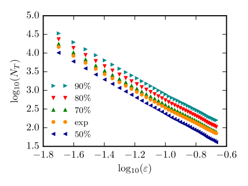
Figure 3: The transport times of Table I as functions of $\varepsilon$ in log-log presentation. They clearly obey power laws, at smaller $\varepsilon<0.1$ with the slope $\approx-2.33$, and at larger $\varepsilon>0.1$ with the slope $\approx-2.1$., while the global fit (ignoring the break point at around $\varepsilon=0.1$) gives $\approx-2.25$. For the precise data see Table II.

Power law exponents for transport times
$N_{T}$	power all $\varepsilon$	error	power $\varepsilon<0.1$	error	power $\varepsilon>0.1$	error
90%	-2.229	0.0101	-2.323	0.0079	-2.092	0.0078
80%	-2.249	0.0084	-2.327	0.0076	-2.142	0.0092
70%	-2.263	0.0072	-2.329	0.0072	-2.178	0.0096
50%	-2.294	0.0048	-2.333	0.0069	-2.259	0.0105
exp	-2.211	0.0117	-2.320	0.0096	-2.053	0.0078

Table 2: The power law exponents (with estimated errors) of $N_{T}$ of Fig. 3 as functions of $\varepsilon$ in log-log presentation: The first two columns refer to the global fit. There is a break point at approximately $\varepsilon\approx 0.1$ where the slopes slightly change. The second pair of columns refers to the interval $\varepsilon<0.1$, and the last two columns refer to the interval $\varepsilon>0.1$.

IV The scaling of $\beta$ and $A$ with $\alpha$

Having established the transport times and the parameter $\alpha$ in Eq. (16) we can now look at the dependence of the level repulsion exponent $\beta$ on $\alpha$ for various definitions of $N_{T}$, from Table I. For each $\beta(\epsilon_{j},(k_{i},k_{i+1}))$ (see Section II) an associated value of $\alpha$ was computed using Eq. (16) where $N_{T}=N_{T}(\epsilon_{j})$ and $k=\bar{k}_{i}=\frac{1}{2}(k_{i}+k_{i+1})$. In Fig. 4, using the $N_{T}$ from the exponential law,

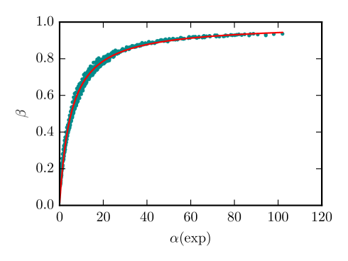
Figure 4: The level repulsion exponent $\beta$ as a function of $\alpha$ fitted by the function (18), based on $N_{T}$ from the exponential diffusion law. $\beta_{\infty}=0.98$ and $s=0.20$.

we clearly see that $\beta$ is a function of $\alpha$, empirically well described by the rational function

$$\beta=\beta_{\infty}\frac{s\alpha}{1+s\alpha}.$$ (18)

where the parameter $s$ depends on the definition of $N_{T}$, as we shall see, and changes with the definition of $N_{T}$ implicit in $\alpha$, but the functional form (18) persists. Here we find $\beta_{\infty}=0.98$ and $s=0.20$, using the $N_{T}$ from the exponential diffusion law.

In the next Fig. 5 we show the dependence of $\beta$ on $\alpha$ using the definitions of the transport time in terms of the fraction of the asymptotic value of the momentum variance. Again, the rational function (18) is confirmed.

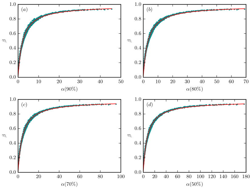
Figure 5: The level repulsion exponent $\beta$ as a function of $\alpha$ fitted by the function (18). For the transport times calculated in Table I, we find for $90\%$, $80\%$, $70\%$ and $50\%$ criterion the corresponding values ($\beta_{\infty},s$) as follows: (a) $(0.98,0.46)$, (b) $(0.98,0.32)$, (c) $(0.98,0.24)$, and (d) $(0.98,0.13)$.

It should be observed that according to the empirical law of Eq. (18), and as seen in both Figs. 4 and 5, the transition from complete localization $\beta=0$ to the full extendedness (delocalization) $\beta\approx 1$ is very smooth, as it happens on the interval of about almost two decades of $\alpha$, rather than being abrupt.

Finally, we look at the dependence of the localization measure $A$, defined in Eqs. (8,9), on $\alpha$. As we see in Fig. 2, $\beta$ is a linear function of $A$, while it is a rational function of $\alpha$. Thus the entropy localization measure $A$ also must be a rational function of $\alpha$, similarly as in Eq. (18), namely

$$A=A_{\infty}\frac{s\alpha}{1+s\alpha}.$$ (19)

Indeed, in Fig. 6 we see that this is the case.

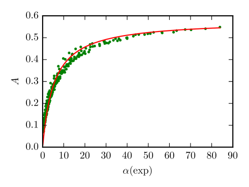
Figure 6: The entropy localization measure $A$ as a function of $\alpha$ fitted by the function (19), based on $N_{T}$ from the exponential diffusion law. $A_{\infty}=0.58$ and $s=0.19$.

In analogy with figures 5 we display also the dependence of $A$ on $\alpha$ for four various definitions of $N_{T}$ from Table I in Fig. 7.

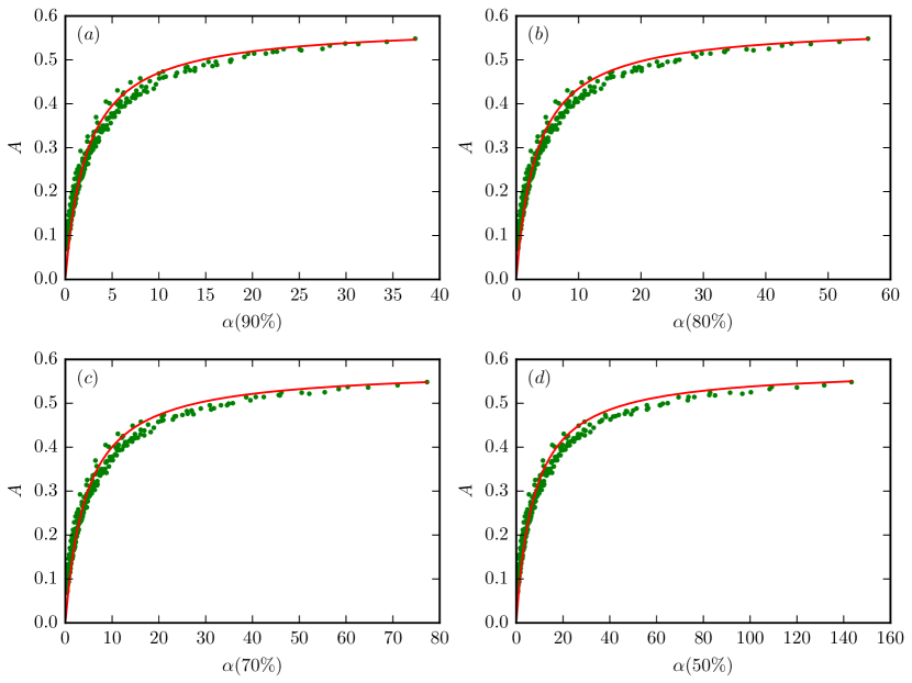
Figure 7: The entropy localization measure $A$ as a function of $\alpha$ fitted by the function (19). For the transport times calculated in Table I, we find for $90\%$, $80\%$, $70\%$ and $50\%$ criterion the corresponding values ($A_{\infty},s$) as follows: (a) $(0.58,0.43)$, (b) $(0.58,0.30)$, (c) $(0.58,0.22)$, and (d) $(0.58,0.13)$.

V Conclusions and discussion

Our main conclusion is that in the stadium billiard of Bunimovich Bunimovich (1979) the spectral level repulsion exponent $\beta$ of the chaotic eigenstates is functionally related to the localization measure, here specifically the entropy localization measure $A$, calculated by using the Poincaré-Husimi functions. Moreover, the dependence is linear, as in the quantum kicked rotator, but different from the case of a mixed type billiard studied recently by Batistić and Robnik Batistić and Robnik (2013a, b), where the high-lying localized chaotic eigenstates have been analyzed after the separation of regular and chaotic eigenstates.

Furthermore, we have shown that $\beta$ is a rational function of the major control parameter $\alpha$, which is the ratio of the Heisenberg time and the classical transport time. The definition of the classical transport time is to some extent arbitrary, but we have shown that the various definitions do not change the shape of the dependence on $\varepsilon$, but instead affect only the prefactor. As a cosequence of that the dependence is always a rational function. The transition from complete localization $\beta=0$ to the complete extendedness (delocalization) $\beta\approx 1$ takes place very smoothly, over about two decades of the parameter $\alpha$.

Thus we have again demonstrated by numerical calculation that the fractional power law level repulsion with the exponent $\beta\in[0,1]$ is manifested in localized chaotic eigenstates. Our empirical findings call for theoretical explanation, which is a long standing open problem even for the main paradigm of quantum chaos, the quantum kicked rotator studied extensively over the decades Izrailev (1990).

Further theoretical work is in progress. Beyond the billiard systems, there are many important applications in various physical systems, like e.g. in hydrogen atom in strong magnetic field Robnik (1981, 1982); Hasegawa et al. (1989); Wintgen and Friedrich (1989); Ruder et al. (1994), which is a paradigm of stationary quantum chaos, or e.g. in microwave resonators, the experiments introduced by Stöckmann around 1990 and intensely further developed since then Stöckmann (1999).

VI Acknowledgement

This work was supported by the Slovenian Research Agency (ARRS) under the grant J1-9112.

References

- Stöckmann (1999) H.-J. Stöckmann, Quantum Chaos - An Introduction (Cambridge: Cambridge University Press, 1999).
- Haake (2001) F. Haake, Quantum Signatures of Chaos (Berlin: Springer, 2001).
- Casati et al. (1979) G. Casati, B. V. Chirikov, F. M. Izrailev, and J. Ford, Lecture Notes in Physics 93, 334 (1979).
- Chirikov et al. (1981) B. V. Chirikov, F. M. Izrailev, and D. L. Shepelyansky, Sov. Sci. Rev. C 2, 209 (1981).
- Chirikov et al. (1988) B. V. Chirikov, F. M. Izrailev, and D. L. Shepelyansky, Physica D 33, 77 (1988).
- Izrailev (1990) F. M. Izrailev, Phys. Rep. 196, 299 (1990).
- Izrailev (1988) F. M. Izrailev, Phys. Lett. A 134, 13 (1988).
- Izrailev (1989) F. M. Izrailev, J. Phys. A: Math. Gen. 22, 865 (1989).
- Fishman et al. (1982) S. Fishman, D. R. Grempel, and R. E. Prange, Phys. Rev. Lett. 49, 509 (1982).
- Prosen (2000) T. Prosen, in Proc. of the Int. School in Phys. ”Enrico Fermi”, Course CXLIII, Eds. G. Casati and U. Smilansky (Amsterdam: IOS Press, 2000).
- Batistić and Robnik (2013a) B. Batistić and M. Robnik, Phys. Rev. E 88, 052913 (2013a).
- Robnik (1983) M. Robnik, J. Phys. A: Math. Gen. 16, 3971 (1983).
- Robnik (1984) M. Robnik, J. Phys. A: Math. Gen. 17, 1049 (1984).
- Batistić and Robnik (2013b) B. Batistić and M. Robnik, J. Phys. A: Math. Theor. 46, 315102 (2013b).
- Bunimovich (1979) L. Bunimovich, Commun. Math. Phys. 65, 295 (1979).
- Borgonovi et al. (1996) F. Borgonovi, G. Casati, and B. Li, Phys. Rev. Lett. 77, 4744 (1996).
- Č. Lozej and Robnik (2018) Č. Lozej and M. Robnik, Phys. Rev. E 97, 012206 (2018).
- Mehta (1991) M. L. Mehta, Random Matrices (Boston: Academic Press, 1991).
- Guhr et al. (1998) T. Guhr, A. Müller-Groeling, and H. Weidenmüller, Phys. Rep. 299, 4 (1998).
- Robnik (1998) M. Robnik, Nonl. Phen. in Compl. Syst. (Minsk) 1, 1 (1998).
- Percival (1973) I. C. Percival, J. Phys B: At. Mol. Phys. 6, L229 (1973).
- Berry and Robnik (1984) M. V. Berry and M. Robnik, J. Phys. A: Math. Gen. 17, 2413 (1984).
- Batistić and Robnik (2010) B. Batistić and M. Robnik, J. Phys. A: Math. Theor. 43, 215101 (2010).
- Casati et al. (1980) G. Casati, F. Valz-Gris, and I. Guarneri, Lett. Nuovo Cimento 28, 279 (1980).
- Bohigas et al. (1984) O. Bohigas, M. J. Giannoni, and C. Schmit, Phys. Rev. Lett. 52, 1 (1984).
- Sieber and Richter (2001) M. Sieber and K. Richter, Phys. Scr. T90, 128 (2001).
- Müller et al. (2004) S. Müller, S. Heusler, P. Braun, F. Haake, and A. Altland, Phys. Rev. Lett. 93, 014103 (2004).
- Heusler et al. (2004) S. Heusler, S. Müller, P. Braun, and F. Haake, J. Phys.A: Math. Gen. 37, L31 (2004).
- Müller et al. (2005) S. Müller, S. Heusler, P. Braun, F. Haake, and A. Altland, Phys. Rev. E 72, 046207 (2005).
- Müller et al. (2009) S. Müller, S. Heusler, A. Altland, P. Braun, and F. Haake, New J. of Phys. 11, 103025 (2009).
- Gutzwiller (1980) M. C. Gutzwiller, Phys. Rev. Lett. 45, 150 (1980).
- Berry (1985) M. V. Berry, Proc. Roy. Soc. Lond. A 400, 229 (1985).
- Brody (1973) T. A. Brody, Lett. Nuovo Cimento 7, 482 (1973).
- Brody et al. (1981) T. A. Brody, J. Flores, J. B. French, P. A. Mello, A. Pandey, and S. S. M. Wong, Rev. Mod. Phys. 53, 385 (1981).
- Manos and Robnik (2013) T. Manos and M. Robnik, Phys. Rev. E 87, 062905 (2013).
- Batistić et al. (2013) B. Batistić, T. Manos, and M. Robnik, EPL 102, 50008 (2013).
- Wigner (1932) E. Wigner, Phys. Rev. 40, 749 (1932).
- Husimi (1940) K. Husimi, Proc. Phys. Math. Soc. Jpn. 22, 264 (1940).
- Tualle and Voros (1995) J. Tualle and A. Voros, Chaos Solitons Fractals 5, 1085 (1995).
- Bäcker et al. (2004) A. Bäcker, S. Fürstberger, and R. Schubert, Phys. Rev. E 70, 036204 (2004).
- Manos and Robnik (2015) T. Manos and M. Robnik, Phys. Rev. E 91, 042904 (2015).
- Santaló and Kac (2004) L. A. Santaló and M. Kac, Integral geometry and geometric probability, Cambridge mathematical library (Cambridge University Press, Cambridge, 2004).
- Robnik (1981) M. Robnik, J. Phys. A: Math. Gen. 14, 3195 (1981).
- Robnik (1982) M. Robnik, J. Phys. Colloque C2 43, 29 (1982).
- Hasegawa et al. (1989) H. Hasegawa, M. Robnik, and G. Wunner, Prog. Theor. Phys. Suppl. (Kyoto) 98, 198 (1989).
- Wintgen and Friedrich (1989) D. Wintgen and H. Friedrich, Phys. Rep. 183, 38 (1989).
- Ruder et al. (1994) H. Ruder, G. Wunner, H. Herold, and F. Geyer, Atoms in Strong Magnetic Fields (Heidelberg: Springer, 1994).