The Simpson’s Paradox in the Offline Evaluation of Recommendation Systems

Abstract.

Recommendation systems are often evaluated based on user’s interactions that were collected from an existing, already deployed recommendation system. In this situation, users only provide feedback on the exposed items and they may not leave feedback on other items since they have not been exposed to them by the deployed system. As a result, the collected feedback dataset that is used to evaluate a new model is influenced by the deployed system, as a form of closed loop feedback. In this paper, we show that the typical offline evaluation of recommender systems suffers from the so-called Simpson’s paradox. Simpson’s paradox is the name given to a phenomenon observed when a significant trend appears in several different sub-populations of observational data but disappears or is even reversed when these sub-populations are combined together. Our in-depth experiments based on stratified sampling reveal that a very small minority of items that are frequently exposed by the deployed system plays a confounding factor in the offline evaluation of recommendation systems. In addition, we propose a novel evaluation methodology that takes into account the confounder, i.e the deployed system’s characteristics. Using the relative comparison of many recommendation models as in the typical offline evaluation of recommender systems, and based on the Kendall rank correlation coefficient, we show that our proposed evaluation methodology exhibits statistically significant improvements of 14% and 40% on the examined open loop datasets (Yahoo! and Coat), respectively, in reflecting the true ranking of systems with an open loop (randomised) evaluation in comparison to the standard evaluation.

1. Introduction

Recommendation systems are typically measured in either an online (A/B testing or interleaving) or an offline manner. However, the offline evaluation of recommender systems remains the most widely reported evaluation in the literature due to the difficulties in deploying research systems for online evaluation (Cañamares et al., 2020; Herlocker et al., 2004). In reality, it is hard to reliably evaluate the effectiveness of a recommendation model in an offline fashion using logs of historical user interactions (Jadidinejad et al., 2019; Chaney et al., 2018; Valcarce et al., 2018). The issue is that there may be confounders, i.e. variables that affect both the exposure of items and the outcomes (e.g. ratings) (Wang et al., 2018). Confounding problems occur when a platform attempts to model user behaviour without taking into account the selection bias in the exposed recommended items (Diaz et al., 2020), leading to unintended consequences. In this situation, it is difficult to distinguish which user interactions stem from the users’ true preferences and which are influenced by the deployed recommender system.

Typically, the offline evaluation of recommendation systems has two stages: (1) gathering a collection of user’s feedback from a deployed system; and (2) the use of such feedback to empirically evaluate and compare different recommendation models. The first stage can be subject to different types of confounders, either initiated by the item selection behaviour of users or through the actions of the deployed recommendation system (Jadidinejad et al., 2020; Chaney et al., 2018; Gruson et al., 2019). For instance, aside from other interaction mechanisms such as search, users are more likely to interact with those items that they have been exposed to. In this way, using historical interactions in the offline evaluation of a new recommender model, where those interactions have been obtained from the deployed recommender system, forms a closed loop feedback (Jadidinejad et al., 2020; Sun et al., 2019), i.e. the deployed recommender system has a direct effect on the collected feedback, which is in turn used for the offline evaluation of other recommendation models. Hence, the new recommendation model is evaluated in terms of how much it tends to mimic the interactions collected by the deployed model, rather than how well it meets the true preferences of users. On the other hand, in an open loop (randomised) scenario, the deployed model is a random recommendation model, i.e. random items are exposed to the users. Therefore, the feedback loop between the deployed model and the new recommendation model is broken and the deployed model has no effect on the collected feedback dataset and, consequently, it has also no effect on the offline evaluation of any new model based on the collected feedback dataset. However, it is naturally not practical to expose users to random items due to the potential for degraded user experience. Therefore, the training and evaluation of recommendation systems based on closed loop feedback is a critical problem.

Simpson’s paradox is a phenomenon in statistics, in which a significant trend appears in several different groups of observational data but disappears or even reverses when these groups are combined together (Pearl, 2014). In recommendation scenarios, the Simpson’s paradox occurs when the association between the exposure (i.e. the recommended items) and the outcome (i.e. the user’s explicit or implicit feedback) is investigated but the exposure and outcome are strongly influenced by a third variable. In statistics, if the observed feedback is a product of Simpson’s paradox, the stratification of the feedback according to the confounding variable causes the disappearance of the paradox. We argue that in the case of recommendation systems, this confounding variable is the deployed model (or system) from which the interaction data were collected, a.k.a. closed loop feedback (Jadidinejad et al., 2020). Our key aims in this paper are to provide an in-depth investigation of the impact of closed loop feedback on the offline evaluation of recommendation systems and to provide a robust solution to the problem. In particular, we argue that the feedback datasets collected from a deployed model are biased towards the deployed model’s characteristics, leading to the conclusions being prone to the Simpson’s paradox. We thoroughly investigate the effect of the confounding variable (i.e. the deployed model’s characteristics) on the offline evaluation of recommendation systems where significant trends are observed, which then disappear or even reverse when reporting observations from the classical offline setting. In addition, we propose a new evaluation methodology that addresses the Simpson’s paradox in order to conduct a sounder offline evaluation of recommendation systems.

To better understand the subtleties of the tackled problem, consider a deployed recommendation model that promotes a specific group of items (e.g. popular items) – there are a few head items that are widely exposed to the users that obtain a large number of interactions, in contrast to a long tail of items with only a few interactions. When we evaluate a new recommendation model based on feedback that was collected from the aforementioned deployed model without taking into account (or adjusting) how frequently different items were exposed, the evaluation process is confounded by the deployed model’s characteristics, i.e. the performance of any model that has a tendency to exhibit similar properties to the already deployed model will likely be over-estimated. In this situation, we might choose to deploy a new model that matches the properties of the already deployed model, while it might be less effective than another model from the actual users’ perspective. In this paper, we thoroughly investigate the consequences of this problem on the conclusions drawn from the standard offline evaluation of recommender systems and propose a new methodology to address the issue. In particular, the contributions of this paper are two-fold:

• We present an in-depth analysis of the standard offline evaluation of recommender systems, showing that it indeed suffers from the Simpson’s paradox. Our in-depth experiments on four well-known closed loop and open loop (randomised) datasets reveal that a very small minority of items that are over-exposed by the deployed model play a confounding factor in a standard offline evaluation, i.e. significant trends in a given recommender system’s performance that are observed in the majority of user-item interactions actually disappear or even reverse in the standard offline evaluation when we merge this majority feedback with a minority confounder.

• To address this problem, we propose a new propensity-based stratified evaluation method in comparison to both the standard offline holdout evaluation (Sammut and Webb, 2010) and the recently introduced counterfactual evaluation (Schnabel et al., 2016; Yang et al., 2018) methods. Our experiments on a broad range of recommendation models and evaluation metrics reveal that the proposed propensity-based stratified evaluation method better represents the actual utility of the examined recommendation models.

The remainder of the paper is organised as follows: In Section 2, we position our contributions in comparison to the existing literature while Section 3 describes the current offline evaluation methods. Section 4 presents the Simpson’s paradox and how it affects the offline evaluation of recommender systems; Section 5 describes the new proposed evaluation method; Section 6 and Section 7 present the experimental setup as well as the conducted experiments and their analysis, respectively. Finally, Section 8 summarises our findings.

2. Related Work

Our work is inspired by three lines of related research, ranging from tackling bias in learning to rank methods (Section 2.1), through algorithmic confounding or closed loop feedback (Section 2.2), to recent work on counterfactual learning and evaluation (Section 2.3).

2.1. Unbiased Learning to Rank

Users’ feedback in recommendation systems is reminiscent of clickthrough data in information retrieval (IR). Previous research (Radlinski et al., 2011) has shown that there is a strong dependency between the documents presented to the user, and those for which the system receives feedback, i.e. higher-ranked documents obtain more clicks (a phenomenon denoted in the literature as position/presentation bias). For example, consider a movie recommendation system that aims to learn the users’ preferences by observing their watching history. The system can infer which movie(s) they prefer over other programs at a particular time, but these are relative preferences in relation to the exposed movies, but do not constitute preferences on an absolute scale. Previous research in information retrieval (IR) (Radlinski et al., 2008, 2011) has revealed that such feedback does not reliably reflect retrieval quality while nonetheless still providing relative user preferences in paired experiments. Classical offline evaluation setups in IR use pooling to gather a comprehensive set of possibly relevant documents for assessment, thereby preventing bias in the relevance assessments towards a single system (known as incompleteness). However, pooling is not a suitable approach for addressing incompleteness in the evaluation of recommendation systems, due to the contextual and personalised nature of users’ recommendation needs.

Recent, unbiased learning to rank approaches aim to learn reliable relevance signals from noisy and biased clickthrough data either with the help of click models or through counterfactual methods (Joachims et al., 2017; Ai et al., 2018b, a; Oosterhuis and de Rijke, 2020). These models typically require a large quantity of clicks, which makes them difficult to apply in systems where click data is highly sparse due to the personalised nature of recommendation systems (Wang et al., 2016; Ovaisi et al., 2020). On the other hand, these models are designed to tackle position/presentation bias in IR systems. However, although both position and presentation bias can influence the collected feedback from a deployed recommendation system, recommendation systems mostly suffer from selection bias (Jadidinejad et al., 2020; Chaney et al., 2018; Jiang et al., 2019). In this paper, we investigate the origin of selection bias in recommendation systems and provide a novel evaluation method that takes into account the role of the deployed recommendation system.

2.2. Algorithmic Confounding

Recommendation systems are often evaluated with interaction data obtained from users that have already been exposed to a deployed algorithm. This creates a feedback loop (Jiang et al., 2019; Sun et al., 2019) (a.k.a. algorithmic confounding (Chaney et al., 2018) or closed loop feedback (Jadidinejad et al., 2020)). Using simulations on synthetic data, Chaney et al. (Chaney et al., 2018) revealed that this feedback loop in recommendation models encourages similar users to interact with the same set of items, thereby homogenising their behavior, relative to an open loop (randomised) platform where random items are exposed to the user. In contrast to the simulation experiments, Jadidinejad et al. (Jadidinejad et al., 2020) investigated the effect of closed loop feedback in both the training and offline evaluation of recommendation models based on an open loop (randomised) dataset. They found that there is a strong correlation between the deployed model from which the users’ feedback were collected and a new model that is trained or evaluated based on the collected feedback dataset. For example, when popular items are favoured by the deployed algorithm, the observed interactions are biased towards popular items. In this situation, the performance of any algorithm that has a tendency to recommend popular items might be over-estimated (Chaney et al., 2018; Jadidinejad et al., 2019, 2020). In this paper, we propose a theoretical framing of feedback loops in recommendation systems based on the Simpson’s paradox, as well as formulate and validate hypotheses about the implications of closed loop feedback in the offline evaluation of recommendation systems. In addition, we propose a novel evaluation methodology, which takes into account the confounding role of the deployed model and show its benefits in comparison to both the standard offline holdout evaluation (Sammut and Webb, 2010) and the recently introduced counterfactual evaluation (Schnabel et al., 2016; Yang et al., 2018) methods.

2.3. Counterfactual Learning and Evaluation

Although researchers in IR have proposed novel approaches for both learning (Joachims et al., 2017) and evaluating (Radlinski et al., 2008, 2011) from user’s clickthrough data, many researchers and practitioners still focus on evaluating recommendation systems in terms of accuracy metrics on datasets that were collected from an already deployed system (Cañamares et al., 2020; Herlocker et al., 2004; Steck, 2010, 2011). On the other hand, several recent studies (Joachims and Swaminathan, 2016; Schnabel et al., 2016; Yang et al., 2018) have attempted to estimate the actual utility of a recommendation model with propensity-weighting techniques commonly used in the off-policy evaluation approaches in Reinforcement Learning with the aim of achieving an unbiased performance estimator of biased observations. Propensity in this context is the probability that the deployed model has exposed item $i$ to user $u$ by the time of feedback collection. The intuition in counterfactual evaluation is that each feedback is individually weighted based on its propensity. The key to a fair evaluation in the counterfactual approaches lies in accurately logging propensities in an open loop (randomised) dataset where random items are exposed to the user. However, most current public recommendation datasets do not introduce a randomisation element (Schnabel et al., 2016; Yang et al., 2018), making it practically difficult to effectively deploy the counterfactual approaches for evaluating recommender systems. In the absence of open loop (randomised) feedback, the estimated propensities are noisy and skewed. As a result, weighting each feedback individually based on its propensity score can lead to a high variance in the estimation of the model’s effectiveness, as reported in several previous studies (Swaminathan and Joachims, 2015; Joachims and Swaminathan, 2016; Schnabel et al., 2016; Yang et al., 2018). Hence, compared to previous works on propensity weighting (Schnabel et al., 2016; Yang et al., 2018), our model does not weight each feedback individually based on its propensity. We instead propose a novel evaluation method based on stratification, which considers each feedback in the corresponding stratum based on the estimated propensities. As a result, as our experiments show, our proposed evaluation method is more robust in coping with these noisy estimated propensities.

3. Offline Evaluation Methods

In this section, we summarise the current offline evaluation methods commonly used in the literature, namely the standard holdout evaluation (Section 3.1) and the counterfactual evaluation (Section 3.2).

3.1. Holdout Evaluation

The purpose of the holdout evaluation (Sammut and Webb, 2010) is to test a model on a different data from what it was trained on. In this method, the dataset is randomly divided into a training set and a test set, the latter being the holdout data. The effectiveness of a model ($\hat{R}$) for the predicted item ranking $\hat{Z}$ can be calculated as follows on the holdout data (Yang et al., 2018):

(1) $$\hat{R}_{\mathrm{holdout}}(\hat{Z})=\frac{1}{|\mathcal{U}|}\sum_{u\in\mathcal{U}}\frac{1}{\left|\mathcal{S}_{u}^{*}\right|}\sum_{i\in\mathcal{S}_{u}^{*}}c(\hat{Z}_{u,i})$$

where $\mathcal{S}_{u}^{*}$ is the set of items (among all the items in $\mathcal{I}$) that are exposed to the user $u\in\mathcal{U}$, $\hat{Z}_{u,i}$ is the predicted ranking of the exposed item $i$ for user $u$, and the function $c$ denotes any top-k scoring metric, such as normalised Discounted Cumulative Gain at rank cutoff k (nDCG@k).

The holdout evaluation method is the standard and most common evaluation method in the field of recommendation systems because of its simplicity and flexibility (Cañamares et al., 2020; Herlocker et al., 2004). However, if the dataset is biased towards a group of items, the holdout test set will be a biased sample of the user-item interactions (Wang et al., 2018). Therefore, the holdout evaluation does not necessarily represent the actual effectiveness of the examined models, i.e. the expected outcome of the holdout evaluation does not necessarily conform to the open loop evaluation (Yang et al., 2018):

(2) $$\mathbb{E}_{O}\left[\hat{R}_{\mathrm{holdout}}(\hat{Z})\right]\neq R(\hat{Z})$$

where $R$ is the actual performance of the predicted ranking of items $\hat{Z}$. In this situation, the effectiveness of any model that captures the bias in the original dataset might be over-estimated (Chaney et al., 2018; Yang et al., 2018). For example, when popular items are favoured by the deployed algorithm, the observed interactions are biased towards popular items. As a result, the performance of any algorithm that has a tendency to recommend popular items might be over-estimated (Jadidinejad et al., 2019). An expensive solution is to create an open loop (randomised) test set from the experiments, i.e. to ask the users to provide feedback for randomly selected items. Another alternative and more practical solution consists in using the propensity-based methods (Austin, 2011) (e.g. counterfactual evaluation), which we describe in the following section.

3.2. Counterfactual Evaluation

The problem of evaluating recommendation models using historical feedback is similar to counterfactual evaluation in reinforcement learning. In this setting, the goal is to evaluate a new recommendation model based on a feedback dataset that is collected from a deployed recommendation model. Inverse Propensity Scoring (IPS) leverages importance sampling to account for the fact that the feedback, which was collected from the deployed recommendation model is not uniformly random. Theoretically, the IPS evaluation method is able to evaluate a new model independently from the deployed model (the confounder). In the context of recommendation systems, the IPS evaluation method was proposed for both explicit (Schnabel et al., 2016) and implicit (Yang et al., 2018) feedback. The key idea of IPS is to reweight feedback based on the propensities of the logged items using importance sampling. The propensity $p_{u,i}$ in this context is the probability that item $i$ would have been shown to the user $u$ by the time the feedback data was collected. The effectiveness of a model ($\hat{R}$) for the predicted item ranking $\hat{Z}$ and the provided propensity scores $P$ can be calculated as follows (Yang et al., 2018):

(3) $$\hat{R}_{\mathrm{IPS}}(\hat{Z}|P)=\frac{1}{|\mathcal{U}|}\sum_{u\in\mathcal{U}}\frac{1}{\left|\mathcal{S}_{u}^{{\color[rgb]{0,0,0}*}}\right|}\sum_{i\in\mathcal{S}_{u}^{*}}\frac{c(\hat{Z}_{u,i})}{p_{u,i}}$$

The intuition behind the IPS method is that the propensity score $p_{u,i}$ is a balancing factor: conditioned on the propensity score, the observed feedback distribution will be adjusted to the examined model. Unlike the holdout evaluation $\hat{R}_{\mathrm{holdout}}$, the IPS evaluation method is theoretically unbiased ($\mathbb{E}_{O}\left[\hat{R}_{\mathrm{IPS}}(\hat{Z})\right]=R(\hat{Z})$) if and only if we can sample open loop feedback from all possible items $\mathcal{I}$ uniformly at random (Swaminathan and Joachims, 2015). However, in various situations, it may be difficult or even impossible to expose users to random items due to obvious business constraints (users are unlikely to tolerate that the system keeps showing them random non-relevant items). Moreover, the imbalance of the assigned propensities will allow for some feedback to be weighted disproportionately. As a result, a major difficulty in applying the IPS evaluation method in practice is its high variance in the estimation of a given model’s effectiveness (Swaminathan and Joachims, 2015). In the following, we investigate the impact of our proposed propensity-based stratified evaluation in comparison to both the holdout and counterfactual evaluation.

4. Simpson’s Paradox

Simpson’s paradox is the name given to an observed phenomenon in statistics, in which a significant trend appears in several different groups of observational data but disappears or even reverses when these groups are combined together. This topic has been widely studied in the causal inference literature (Pearl, 2014; Kievit et al., 2013). In this phenomenon, an apparent paradox arises because aggregated data can support a conclusion that is opposite to the conclusions from the same stratified data before aggregation. The Simpson’s paradox occurs when the association between two variables is investigated but these variables are strongly influenced by a confounding variable. When the data is stratified according to the confounding variable, the paradox is revealed showing paradoxical conclusions. In this situation, the use of a significance test might identify unsound conclusions made across a specific stratum; however, as we show later in Section 7, significance tests may not possibly identify such trends. Indeed, in a recommender system evaluation scenario, testing occurs over users, while the paradox we discuss here usually involves the user-item feedback generation process. On the other hand, the Simpson’s paradox can be resolved when causal relations are appropriately addressed in statistical modeling (Pearl, 2014).

Table 1. Simpson’s paradox examples in medical studies (a) and recommendation systems (b).

(a) Kidney stone example (Charig et al., 1986). Each entry represents the number of responses out of the total number of patients while the success rates are shown in brackets.

	Treatment A	Treatment B
Size $<$ 2cm	Group 1	Group 2
	081/870 (93%)	234/270 (87%)
Size $\geq$ 2cm	Group 3	Group 4
	192/263 (73%)	055/800 (69%)
Both	273/350 (78%)	289/350 (83%)

(b) Simpson’s paradox in the offline evaluation of recommender systems. Each entry represents the effectiveness of the examined model on the corresponding stratum. * denotes a significant difference compared to the other model (paired t-test, p ¡0.05).

	***Model A***	***Model B***
Q1 (99%)	Group 1	Group 2
	0.339	0.350*
Q2 (1%)	Group 3	Group 4
	0.695*	0.418
Both	0.373*	0.369

In this section, to illustrate the Simpson’s paradox, we present a real-life example from a seminal paper (Charig et al., 1986) comparing the success rates of two treatments for the kidney stone disease. The objective is to find out which treatment is more effective based on observational studies. Charig et al. (Charig et al., 1986) randomly sampled 350 patients who were exposed to each treatment and reported the success rates in Table 1(a). A plausible conclusion is that treatment B is more effective than treatment A (83% vs. 78% recovery rate). On the other hand, the paradoxical conclusion is that the success rates reverse when the stone size is taken into account, i.e. treatment A is more effective for both small (93% vs. 87%) and large stone sizes (73% vs. 69%). Charig et al. (Charig et al., 1986) argued that the treatment (A vs. B) and the outcome (success vs. failure) are strongly associated with a third confounding variable (namely, the stone size):

Hypothesis 1.

Doctors tend to opt for favoring treatment B for less severe cases (i.e. small stones) while favouring treatment A for more severe cases (i.e. large stones).

Table 1(a) (data from (Charig et al., 1986)) validates the above hypothesis, i.e. the majority of patients who were exposed to treatment A had large stones (263 out of 350 random patients in Group 3) while the majority of patients who were exposed to treatment B had small stones (270 out of 350 random patients in Group 2). As a result, when the samples are randomly selected from the patients who were exposed to treatments A or B, the sampling process is not purely random, i.e. the samples are systematically skewed towards the patients who have severe cases for measuring treatment A, while sampling mild cases for measuring treatment B. This is a well-known phenomena in causal analysis, which is also known as the Simpson’s paradox (Pearl, 2014).

Table 1(b) shows an illustrative example of the Simpson’s paradox in the offline evaluation of recommendation systems. We are interested to evaluate the effectiveness of two recommendation models, depicted as A and B in Table 1(b). Both models are evaluated on the same dataset and using the same evaluation metric. The standard offline evaluation on the examined dataset shows that model A significantly outperforms model B, according to a paired t-test. However, stratifying the examined dataset into two strata (Q1 and Q2) reveals that indeed model B is the significantly better model for 99% of the examined dataset while model A is statistically superior only for a small minority (1%) of the examined dataset. The statistical superiority of model B in 99% of the examined dataset disappears when aggregating the Q1 and Q2 strata together. In the following section, we present how the Simpson’s paradox affects the offline evaluation of recommendation systems, discuss the causes of such a paradox and propose a new evaluation methodology to address it.

5. Propensity-based Stratified Evaluation

(a) Data flow in a recommender system (Jadidinejad et al., 2020).

(b) Assumed coarse-grained causal diagram.

Figure 1. Closed loop feedback in recommendation systems.

When creating a dataset for the offline evaluation of a recommender system, the users’ feedback can be collected not only from interactions with items suggested by the deployed recommendation system but also through other modalities such as interactions occurring when browsing the items’ catalogue or when following links to sponsored items. It is not straightforward to distinguish the source of the users’ feedback since no public datasets provide sufficient data to establish the sources of the users’ feedback. Hence, in this paper we focus our investigation on the main source of user’s feedback, namely the deployed system (Chaney et al., 2018; Jiang et al., 2019; Jadidinejad et al., 2019; Anderson et al., 2020). In order to demonstrate the Simpson’s paradox in recommendation systems, we need a causal hypothesis similar to Hypothesis 1 in Section 4.

Figure 1(a) shows the information flow of a typical recommendation system where the users’ feedback is collected through the deployed system. The deployed recommender system component (denoted by RecSys) filters items for the target user (e.g. by suggesting a ranked list of items) depicted as the exposure ($e$). On the other hand, the user’s recorded preferences (e.g. ratings or clicks) towards items (depicted as $r$) are leveraged as interaction data to train and/or evaluate the next-generation of the recommendation model. Hence, since the users’ clicks are obtained on items exposed by the RecSys, the model itself influences the generation of data that is used to either train or evaluate it (Jiang et al., 2019). The system presented in Figure 1(a) is a dynamic system where a simple associative reasoning about the system is difficult because each component influences the other. Figure 1(b) shows the corresponding causal diagram in such a closed loop feedback scenario. The solid lines represent an explicit/observed relationship between the causes and effects while the dashed line represents an implicit/unobserved relationship. As mentioned above, in the case of recommendation systems, the main confounding variable is the deployed model from which the interaction data were collected (Chaney et al., 2018; Jiang et al., 2019; Jadidinejad et al., 2019). Our aim is to evaluate the effectiveness of a recommendation model ($Y$) based on closed loop feedback ($r$) collected from a deployed model while the analysis is influenced by the main confounder, i.e. the deployed model’s characteristics. In this situation, it is difficult to distinguish those users’ interactions that stem from the users’ true preferences from those that are influenced by the deployed recommendation model. As a result, in the scenario where the users’ feedback is typically collected through the deployed system we postulate that the offline evaluation of recommendation models based on closed loop feedback datasets is strongly influenced by the underlying deployed recommendation model:

Hypothesis 2.

Closed loop feedback collected from a deployed recommendation model is skewed towards the deployed model’s characteristics (i.e. the exposed items) and the deployed model’s characteristics play a confounding factor in the offline evaluation of recommendation models.

The core problem is that the deployed recommendation model is attempting to model the underlying user preferences, making it difficult to make claims about user behaviour (or use the behaviour data) without accounting for algorithmic confounding (Chaney et al., 2018; Jiang et al., 2019). On the other hand, if the RecSys component in Figure 1(a) is a random model, then the interconnection between the User and the RecSys components in Figure 1(a) will be removed and the RecSys component has no effect on the collected feedback dataset, a situation known as open loop feedback, i.e. no item receives more or less expected exposure compared to any other item in the collection (Diaz et al., 2020).

As shown in Figure 1(b), if the deployed model’s characteristics ($e$) could be identified and measured, the offline evaluation ($Y$) would be independent of the confounder. Therefore, in order to validate the effect of closed loop feedback in a recommendation system (Hypothesis 2), we have to quantify the deployed model’s characteristics. To this end, following (Austin, 2011; Yang et al., 2018), we define the propensity score as follows:

Definition 5.1.

The propensity score $p_{u,i}$ is the tendency of the deployed model (depicted as RecSys in Figure 1(a)) to expose item $i\in\mathcal{I}$ to user $u\in\mathcal{U}$.

The propensity $p_{u,i}$ is the probability that item $i$ is exposed to user $u$ by the deployed model under a closed loop feedback scenario. This value quantifies a system’s deviation from an unbiased open loop exposure scenario, where random items are exposed to the user and the deployed model has no effect on the collected feedback. The propensity score $p_{u,i}$ allows us to design and analyse the offline evaluation of recommendation models based on the observed closed loop feedback so that it mimics some of the particular characteristics of the open loop scenario.

Stratification is a well-known approach to identify and estimate causal effects by first identifying the underlying strata before investigating causal effects in each stratum (Austin, 2011). The general intuition is to stratify on the confounding variable and to investigate the potential outcome in each stratum. As a result, it becomes possible to measure the potential outcome irrespective of the confounding variable. In this situation, a marginalisation over the confounding variable can be leveraged as a combined estimate. As mentioned before, the hypothetical confounding variable in recommender systems is the deployed model’s characteristics (Hypothesis 2). Definition 5.1 quantifies this variable as propensities. In this situation, stratification on the propensity scores allows us to analyse the effect of the deployed model’s characteristics on the offline evaluation of recommendation models.

For the sake of simplicity, suppose that we have a single categorical confounding variable $\mathrm{X}$. If we stratify the observed outcome based on the possible values of $\mathrm{X}$, then the expected value of the potential outcome ($\mathrm{Y}$) is defined as follows:

(4) $$\mathrm{E}(\mathrm{Y})=\sum_{x}\mathrm{E}\left(\mathrm{Y}|\mathrm{X}=x\right)\mathrm{P}(\mathrm{X}=x)$$

where $\mathrm{E}\left(\mathrm{Y}|\mathrm{X}=x\right)$ is the conditional expectation of the observed outcome given stratum $x$, and $\mathrm{P}(\mathrm{X}=x)$ is the marginal distribution of $x$. For example, in the kidney stone example presented in Table 1(a), the confounding variable is the kidney stone size based on which our observations were stratified ($X=\{small,large\}$) and the potential outcome is the treatment effect. We can calculate the expected value of each treatment based on Equation (4). For example, the expected value of treatment A can be calculated as follows:

(5) $$\mathrm{E}(\mathrm{A})=\mathrm{E}\left(\mathrm{A}|\mathrm{X}=small\right)\mathrm{P}(\mathrm{X}=small)+\mathrm{E}\left(\mathrm{A}|\mathrm{X}=large\right)\mathrm{P}(\mathrm{X}=large)$$

Based on the numbers in Table 1(a) and Equation (5), the expected value of treatment A (resp. B) is calculated to be 0.832 and 0.782, respectively, i.e. $\mathrm{E}(\mathrm{A})>\mathrm{E}(\mathrm{B})$, which better estimates the actual performance of the treatments. In a similar manner, for the recommendation example in Table 1(b), the expected values of model A and model B are calculated to be 0.343 and 0.351, respectively, i.e. $\mathrm{E}(\mathrm{B})>\mathrm{E}(\mathrm{A})$. As mentioned above, in recommender systems, the main hypothetical confounding variable is the deployed model (Hypothesis 2). This variable is quantified as propensity scores (Definition 5.1). Propensity is a continuous variable. In this paper, we cast it into a categorical variable by sorting and segmenting the propensity scores into a predefined number of strata, i.e. Q1 and Q2 strata in Table 1(b). In both cases of Tables 1(a) and  1(b), stratification based on the hypothetical confounding variable and marginalisation on the examined strata using Equation (4), does resolve the Simpson’s paradox. For example, in Table 1(b), model B should be recognised as the superior model by any reasonable evaluation outcome since it performs better than model A for 99% of the user-item feedback on the examined dataset. This important trend is captured by the proposed stratified evaluation while it is completely reversed in the standard offline evaluation when combining the Q1 and Q2 strata together. In the following section, we investigate the effect of the Simpson’s paradox and the usefulness of our proposed propensity-based stratified evaluation in the offline evaluation of recommendation systems. Specifically, we investigate the following research questions:

Research Question 1.

To what extent is the offline evaluation of recommendation systems affected by the deployed model’s characteristics in a closed loop feedback scenario?

Here, our objective is to assess the confounding effect of the deployed model’s characteristics on the offline evaluation of recommendation models, as depicted in Figure 1(b). In this regard, similar to the schematic examples presented in Section 4, we are interested to stratify the observed closed loop feedback based on the deployed model’s characteristics. Such a stratified analysis enables us to assess the presence of the Simpson’s paradox in the standard offline evaluation of recommendation systems. As such, we investigate significant trends in the relative performances of many different recommendation models where a trend is observed in the majority of strata, but the trend disappears or even reverses in the standard offline evaluation.

Research Question 2.

Can the propensity-based stratified evaluation help in better estimating the actual model’s performance when conducting a comparative offline evaluation?

Our objective in the above research question is to assess the effectiveness of the proposed propensity-based stratified evaluation in the offline evaluation of recommendation models. As shown in Equation (4), we can leverage marginalisation over the distribution of the confounding variable as a combined estimation of the potential outcome. In this research question, we are interested to assess how well this estimation is correlated with the open loop (randomised) evaluation where the deployed model is a random recommendation model, i.e. random items are exposed to the user. Specifically, given a particular evaluation method (open loop, closed loop, etc.) we measure the effectiveness of many recommendation models based on standard rank-based evaluation metrics (e.g. nDCG) and record the relative ranking of those models in terms of the used metric. We then investigate the correlation between the relative rankings of the examined models, comparing the rankings obtained from an open loop (randomised) setup to those obtained using our proposed propensity-based evaluation method. We leverage suitable significance tests, as described in Section 6, to determine if the comparative performances of the examined models predicted by the proposed propensity-based stratified evaluation method better correlates with the open loop (randomised) evaluation in comparison to the standard offline holdout evaluation. Answering this research question provides a better understanding about the actual effectiveness of a given recommendation model in a closed loop scenario.

6. Experimental Setup

Figure 2. The dependent correlations significance test based on Steiger’s method (Steiger, 1980). The effectiveness of each evaluation method ($Y$ and $Z$) is measured based on Kendall’s $\tau$ rank correlation with the open loop (randomised) evaluation ($X$). The significance difference between the baseline evaluation method ($Y$) and the proposed evaluation method ($Z$) is measured based on Steiger’s method (Steiger, 1980).

In the following, we conduct experiments to address the two aforementioned research questions. Figure 2 presents the general structure of our experiments. Each evaluation method ($X$, $Y$ and $Z$) ranks various examined recommendation models based on their relative performances. We use Kendall’s $\tau$ rank correlation coefficient to measure the correlation between the relative order of the examined models in each evaluation method ($Y$ or $Z$) in comparison to the ground truth, i.e. open loop (randomised) evaluation ($X$). These correlation values are depicted as $\tau_{XY}$ and $\tau_{XZ}$ in Figure 2. In addition, we use Steiger’s method (Steiger, 1980) to test the difference between two evaluation methods for significance, e.g. the baseline evaluation method ($Y$) and the proposed evaluation method ($Z$). We compare the effectiveness of our proposed propensity-based stratified evaluation with both the standard offline holdout and the counterfactual evaluation methods as baselines. In the following, we describe the details of our experimental setup including the used datasets and evaluation metrics (Section 6.1), the examined recommendation models (Section 6.2) and how we estimate the propensities (Section 6.3) in our experiments.

6.1. Datasets and Evaluation Metrics

We use four datasets, which are widely used in the offline evaluation of recommendation system, namely the MovieLens (Harper and Konstan, 2015), Netflix (Koren et al., 2009), Yahoo! music rating (Marlin and Zemel, 2009) and Coat shopping (Schnabel et al., 2016) datasets. MovieLens contains 1m ratings from 6k users and 4k items, Netflix contains 607k ratings from 10k users and 5k items, while the Yahoo! dataset contains 300K ratings given by 15.4k users for 1k items. Furthermore, the Coat shopping dataset simulates the shopping for a coat in an online store. It contains about 7k ratings given by 290 users for 300 items. All datasets were collected from an unknown deployed recommendation system in a closed loop scenario. In addition, the Yahoo! dataset has a unique feature: a subset of users (5.4k) were asked to rate 10 randomly selected items (open loop scenario). Therefore, for a subset of users (5.4k), we have both the closed loop and open loop (random) feedback. Similarly, for the Coat dataset, each user was asked to provide ratings for 24 self-selected (closed loop) items and 16 randomly picked (open loop) items. However, in a real-world practical evaluation setup, the training of the models should be based on the collected closed loop feedback, while the actual evaluation could be based on the open loop (random) feedback because of the difficulties of collecting open loop feedback in the real-world, as discussed in Section 1. We use the normalised Discounted Cumulative Gain (nDCG@k) metric for different cut-offs ($k=\{5,10,20,30,100\}$), while we use nDCG, without a rank cutoff, to denote the case where the metric is computed on the ranking of all items for each user. The user’s rating value for all datasets is an integer $r\in[0,5]$. Our objective is to rank the most relevant items for each user. Hence, we binarise all explicit rating values by keeping the highly recommended items ($r\geq 4$). In the closed loop evaluation of the examined models, we use 80% of the closed loop dataset (MovieLens, Yahoo! and Coat) for training and a 20% random split for testing, as is typical in RecSys evaluation (Cañamares et al., 2020). On the other hand, for the open loop evaluation (Yahoo! and Coat), we evaluate the trained models on all the provided open loop (randomised) feedback.

6.2. Recommendation Models

In our experiments, we use the implementations provided by the Cornac framework to evaluate the following models:

• BO: a simple baseline model that recommends a random permutation of all available items to each user, regardless of their preferences.

• GA: a baseline model that recommends the global average rating to each and every user, regardless of their preferences.

• POP: a baseline model that ranks items based on their popularity, i.e. the number of times a specific item is rated, and suggests these items to every user regardless of their preferences.

• MF: Matrix Factorisation (Koren et al., 2009) is a rating prediction model that represents both users and items as latent vectors. This model is optimised to predict the observed rating for each user-item pair.

• PMF: Probabilistic Matrix Factorisation (Salakhutdinov and Mnih, 2007) is an extension of Matrix Factorisation (Koren et al., 2009) for large, sparse and imbalanced datasets. There are two variants of this algorithm depending on how the users’ preferences are modelled, i.e. linear and non-linear. We use both linear and non-linear variants in our experiments.

• SVD++: Singular Value Decomposition (Koren, 2008) is another rating prediction model that factorises the user-item rating matrix to a product of two lower rank matrices, i.e. user factors and item factors.

• WMF: Weighted Matrix Factorisation (Hu et al., 2008) is another extension of Matrix Factorisation (Koren et al., 2009) that models confidence and uncertainty in addition to preferences.

• NMF: Non-negative Matrix Factorisation (Lee and Seung, 2000) factorises the user-item rating matrix into user and item latent matrices, with the property that all matrices have no negative elements.

• BPR: Bayesian Personalised Ranking (Rendle et al., 2009) is a pair-wise ranking model. The BPR model is trained based on uniform negative sampling, i.e. we randomly sample items not interacted with as negative instances for each user. We use both normal and weighted variants in our experiments.

• MMMF: Maximum Margin Matrix Factorisation (Weimer et al., 2008) is a type of matrix factorisation model that is optimised for a soft margin (Hinge) ranking loss.

• NCF: Neural Collaborative Filtering (He et al., 2017) is a general neural network framework for collaborative filtering. We use Multi-Layer Perceptron (MLP), Generalised Matrix Factorisation (GMF) and Neural Matrix Factorisation (NeuMF) in our experiments.

We are interested in the relative order of the models’ performances within closed loop and open loop scenarios. Therefore, following previous research (Gruson et al., 2019), we vary the hyperparameter controlling the size of the latent factors in {10, 20, …, 100}, for each model that supports this hyperparameter. This leads to a total of 104 models that are evaluated in our experiments. Each examined model differs on the algorithm or the latent variable size. When discussing a particular model, we denote the hyperparameter value in superscript - e.g. MF⁴⁰ represents the MF model using latent factor size $m=40$. For reproducibility, our code and the used datasets are available from: https://github.com/terrierteam/stratified_recsys_eval.

6.3. Estimating Propensity Scores

The propensity score $p_{u,i}$ is defined as the tendency of the deployed model to expose item $i$ to user $u$ (Definition 5.1). Since it is not realistic for the deployed model to expose each and every item to the user, we have to estimate the propensity scores $p_{u,i}$ for various user and item pairs. Yang et al. (Yang et al., 2018) proposed a simple method to estimate the propensity scores based on the following simplified assumption:

Assumption 1.

The propensity score is user independent, i.e. $p_{u,i}=p_{*,i}$. This assumption was made to address the lack of auxiliary user information in public datasets.

The user independent propensity score $p_{*,i}$ can be estimated using a two-step generative process (Yang et al., 2018):

(6) $$p_{*,i}=p_{*,i}^{select}*p_{*,i}^{interact|select}$$

where $p_{*,i}^{select}$ is the prior probability that item $i$ is recommended by the deployed model and $p_{*,i}^{interact|select}$ is the conditional probability that the user interacts with item $i$ given that it is recommended. Based on a set of mild assumptions, we can estimate the user independent propensity score $p_{*,i}$ as follows (Yang et al., 2018):

(7) $$\hat{p}_{*,i}\propto\left(n_{i}^{*}\right)^{\left(\frac{\gamma+1}{2}\right)}$$

where $n_{i}^{*}$ is the total number of times item $i$ is interacted with and $\gamma$ is a parameter that affects the propensity distributions over items with different observed popularity. The power-law parameter $\gamma$ affects the propensity distributions over items and depends on the examined dataset. Following previous research (Alstott et al., 2014), we estimate the $\gamma$ parameter using maximum likelihood for each dataset.

7. Experimental Results and Analysis

We proposed a propensity-based stratified evaluation method in Section 5 that takes into account the confounding role of the deployed model in the offline evaluation of recommendation systems. In Section 6, we proposed to use Kendall’s $\tau$ correlation coefficient to quantify the similarity between the relative order of many examined recommendation models in the proposed propensity-based stratified evaluation method as well as in the open loop (randomised) evaluation. In the following, we conduct experiments with respect to the two research questions stated in Section 5, concerning the existence of the Simpson’s paradox in the standard offline evaluation (Section 7.1) and the effectiveness of the proposed propensity-based stratified evaluation method (Section 7.2).

7.1. RQ 1: Investigating Simpson’s Paradox

Table 2. An instance of Simpson’s paradox in the offline evaluation of recommender systems using nDCG on the MovieLens dataset (Harper and Konstan, 2015). * denotes a significant difference compared to the other model (paired t-test, p ¡0.05).

Evaluation Method	BPR10	WMF10	Number of Ratings	Number of Items
Holdout	0.373*	0.369*	200,018	3,449
IPS	0.207*	0.204*	200,018	3,449
Stratified	0.344*	0.351*	200,018	3,449
Q1	0.339*	0.350*	197,600 (99%)	3,445
Q2	0.695*	0.418*	2,418 (1%)	4

Table 3. An instance of Simpson’s paradox in the offline evaluation of recommender systems using nDCG on the Netflix dataset (Koren et al., 2009). * denotes a significant difference compared to the other model (paired t-test, p ¡0.05).

Evaluation Method	MMMF100	MF50	Number of Ratings	Number of Items
Holdout	0.269*	0.263*	121,460	3,962
IPS	0.246*	0.245*	121,460	3,962
Stratified	0.239*	0.241*	121,460	3,962
Q1	0.236*	0.242*	109,452 (90%)	3,944
Q2	0.271*	0.229*	12,008 (10%)	18

Research Question 1 investigates the confounding effect of the deployed model on the offline evaluation of recommendation systems based on closed loop feedback datasets as mentioned in Hypothesis 2. In Section 6.3, we presented a simple statistical method to represent the deployed model’s characteristics as propensity scores. In the following, we use the estimated propensity scores $\hat{p}_{*,i}$ to partition the examined dataset into two equal size strata, namely the Q1 and Q2 strata. Since we estimate the propensity scores based on the total number of times each item is interacted with according to Equation (7), the Q1 and Q2 strata represent the users’ interactions with the long-tail and head items, respectively.

First, we highlight some instances of the Simpson’s paradox in both the examined closed loop (MovieLens and Netflix) and open loop (Yahoo! and Coat) datasets. Tables 2 & 3 compare the effectiveness of the examined evaluation methods (namely the holdout, IPS and our proposed stratified evaluation methods) on the MovieLens and Netflix datasets. For the sake of simplicity, in the following, we focus on the Movielens dataset, analysing two models (BPR¹⁰, WMF¹⁰) and one metric (nDCG). We observe that BPR¹⁰ is significantly better than WMF¹⁰ using both the holdout and counterfactual (IPS) evaluation methods. However, the stratified analysis on the same test dataset (Q1 and Q2 strata) reveals that WMF¹⁰ is significantly better than BPR¹⁰ for the Q1 stratum while BPR¹⁰ is the dominant model for the Q2 stratum. In addition, we observe that the Q1 and Q2 strata cover 99% and 1% of the user-item interactions, respectively. In fact, WMF¹⁰ is significantly better than BPR¹⁰ for 99% of the examined test dataset (i.e. the Q1 stratum) but this trend reverses when we combine it with the 1% feedback in the Q2 stratum, as represented in the holdout evaluation. Therefore, the real question is whether BPR¹⁰ does perform better than WMF¹⁰ as recognised by the holdout evaluation method? The stratified analysis reveals that WMF¹⁰ should be recognised as the superior model by any reasonable evaluation method as recognised by our proposed stratified evaluation. We note that BPR¹⁰ is the superior model only for 1% of the feedback dataset and both the holdout and IPS evaluation methods are influenced by a very small minority of user-item interactions in the test dataset, i.e. 1% of user-item interactions in the Q2 stratum. This stratum corresponds to only 4 items among 3,499 items in the MovieLens dataset. The same pattern is also observed for the Netflix dataset between the MMMF¹⁰⁰ and MF⁵⁰ models presented in Table 3.

Table 4. An instance of Simpson’s paradox in the offline evaluation of recommender systems using nDCG on the Yahoo! dataset (Marlin and Zemel, 2009). * denotes a significant difference compared to the other model (paired t-test, p ¡0.05).

Evaluation Method	BPR40	MF40	Number of Ratings	Number of Items
Holdout	0.270*	0.266*	62,341	1,000
IPS	0.238*	0.239*	62,341	1,000
Stratified	0.249*	0.256*	62,341	1,000
Q1	0.218*	0.250*	57,467 (92%)	995
Q2	0.622*	0.330*	4,874 (8%)*	5
Open Loop	0.169*	0.172*	54,000	1,000

Table 5. An instance of Simpson’s paradox in the offline evaluation of recommender systems using nDCG on the Coat dataset (Schnabel et al., 2016). * denotes a significant difference compared to the other model (paired t-test, p ¡0.05).

Evaluation Method	GMF20	SVD20	Number of Ratings	Number of Items
Holdout	0.245*	0.244*	1,392	286
IPS	0.235*	0.237*	1,392	286
Stratified	0.227*	0.230*	1,392	286
Q1	0.199*	0.215*	1,301 (93%)	281
Q2	0.612*	0.434*	**91 (7%)*	5
Open Loop	0.248*	0.264*	1,392	286

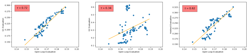
(a) Yahoo! Dataset

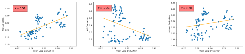
(b) Coat Dataset

Figure 3. The correlation of the examined models between the open loop evaluation (x axis) and the specified closed loop evaluation (y axis) in the Yahoo! dataset (a) and the Coat dataset (b). All Kendall’s $\tau$ correlations are statistically significant according to Steiger’s method (Steiger, 1980) (p ¡0.05). The orange line represents the best fit for the open/closed loop data based on a linear regression model.

In the MovieLens and Netflix datasets, we do not have access to open loop feedback, i.e. feedback that was collected from a randomised exposure to items. As a result, we cannot measure the actual performances of the models in an open loop scenario in comparison to the corresponding closed loop scenario. As mentioned in Section 6.1, we have some open loop feedback for all the users in the Coat dataset and a fraction of users in the Yahoo! dataset. Tables 4 and 5 present performance comparisons of two pairs of models on the Yahoo! and Coat datasets. In particular, in Table 4, we compare BPR⁴⁰ and MF⁴⁰ using the nDCG evaluation metric, and observe that BPR⁴⁰ is significantly better than MF⁴⁰ using the classical holdout evaluation method. On the other hand, the IPS evaluation method favours MF⁴⁰ but the difference is not significant based on the paired t-test ($p<0.05$). However, the stratified analysis based on the estimated propensities (the Q1 and Q2 strata) reveals that MF⁴⁰ is significantly better than BPR⁴⁰ for the Q1 stratum, which covers 92% of feedback in the examined test dataset while BPR⁴⁰ is the dominant model for the Q2 stratum, which covers only 8% of feedback in the closed loop test dataset. Indeed, MF⁴⁰ significantly outperforms BPR⁴⁰ for the majority of feedback and items (92% and 99.5%, respectively) in the examined test dataset. Therefore, we argue that MF⁴⁰ should be recognised as a better model by any reasonable evaluation method as recognised by the proposed stratified evaluation method and the open loop evaluation where random items were exposed to the users. When we evaluate the models based on the aggregation of the Q1 and Q2 strata (i.e. holdout evaluation), a small minority of 5 items out of 1,000 total items corresponding to only 8% of the total user-item interactions in the Yahoo! dataset, plays a confounding factor in the offline evaluation of the examined models. When considering the Coat dataset (Table 5), we also observe the same phenomenon when assessing the effectiveness of the GMF²⁰ and SVD²⁰ recommendation models. The observed phenomenon in Table 2, Table 4 and Table 5 can be explained by the fact that all the examined datasets (MovieLens, Netflix, Yahoo! and Coat) were collected from a closed loop scenario. Therefore, the collected closed loop dataset is skewed towards the deployed model’s characteristics (as captured in the Q2 stratum in Table 2, Table 4 and Table 5).

Next, to fully answer Research Question 1, we assess the generalisation of the above observations, by verifying the prevalence of the Simpson’s paradox in the evaluation of all our 104 models. Figure 3 shows the correlation of all the examined models (104 models as described in Section 6.1) between the open loop evaluation and the specified closed loop evaluation for both the Yahoo! and Coat datasets. We observe that the models exhibit an imbalanced performance on the Q1 and Q2 strata, i.e. the nDCG scores for the Q1 stratum are not in proportion to the Q2 stratum ($nDCG_{Q2}\gg nDCG_{Q1}$). On the other hand, the Kendall’s $\tau$ correlation between the Q1 stratum and the open loop evaluation is much higher compared to the corresponding Q2 stratum ($\tau_{Q1}\gg\tau_{Q2}$). Specifically, for the Coat dataset (Figure 3(b)), the closed loop evaluation based on the Q2 stratum has a negative correlation with the open loop evaluation. As a result, combining these two heterogeneous strata in the holdout evaluation – as shown in Figure 3(a) and Figure 3(b) – without taking into account that the Q1 stratum covers the majority of feedback (92% and 93% of the total feedback in the Yahoo! and Coat datasets, respectively), leads to unexpected consequences. In particular, the Kendall’s $\tau$ correlation between the open loop evaluation and the holdout evaluation is significantly lower than the corresponding correlation between the Q1 stratum and the open loop evaluation, i.e. $0.62<0.72$ and $0.20<0.51$ for the Yahoo! and the Coat datasets, respectively. This answers Research Question 1: the offline holdout evaluation of recommendation systems is influenced by the deployed model’s characteristics (as captured in the Q2 stratum), leading to a conclusion prone to the Simpson’s paradox.

To summarise, in this section, we highlighted the existence of the Simpson’s paradox in the standard offline evaluation of recommendation systems based on both closed loop (MovieLens and Netflix) and open loop (Yahoo! and Coat) datasets. In the following, we investigate the effectiveness of our proposed propensity-based stratified evaluation in addressing the issue.

7.2. RQ 2: Assessing the Proposed Propensity-based Stratified Evaluation Method

In this section, we investigate the extent to which the proposed propensity-based stratified evaluation method (Section 5) leads to conclusions that are aligned with the results obtained from the open loop (randomised) evaluation, compared with both the counterfactual (IPS) and the holdout evaluation methods (Section 3). Indeed, our objective is to investigate to what extent each evaluation method correlates with the open loop evaluation. In contrast, we consider open loop evaluation to be more akin to online evaluation (A/B testing or interleaving) where the evaluation process is not influenced by any confounders. As mentioned in Section 6.2, we make use of the Kendall’s $\tau$ rank correlation coefficient between the examined evaluation method and the open loop evaluation for all the examined recommendation models.

Table 6. Kendall’s $\tau$ rank correlation coefficient between the examined evaluation methods and the open loop (randomised) evaluation on the Yahoo! (Marlin and Zemel, 2009) and Coat (Schnabel et al., 2016) datasets. ^1/2/3/4/5 denote a significant difference compared to the indicated evaluation method (Steiger’s method (Steiger, 1980), p ¡0.05).

Dataset	Metric	Holdout1	IPS2	Stratified3	Q14	Q25
Yahoo!	nDCG@5	*0.5993/4/5/0	0.6414/5/0/0	0.7001/4/5/0	0.4071/2/3/0	*0.4141/2/3/0
	nDCG@10	*0.6934/5/0/0	0.7044/5/0/0	0.6974/5/0/0	0.5591/2/3/0	*0.5011/2/3/0
	nDCG@20	*0.7294/5/0/0	0.7214/5/0/0	0.7164/5/0/0	0.6361/2/3/0	*0.5231/2/3/0
	nDCG@30	*0.6523/5/0/0	0.6533/5/0/0	0.7131/2/5/0	0.6735/0/0/0	*0.4501/2/3/4
	nDCG@100	*0.7013/4/5/0	0.7243/5/0/0	0.7741/2/5/0	0.7731/5/0/0	*0.3481/2/3/4
	nDCG	*0.6223/4/5/0	0.6443/4/5/0	0.7101/2/5/0	0.7221/2/5/0	*0.3361/2/3/4
Coat	nDCG@5	-0.0403/4/5/0	0.0513/4/5/0	0.1161/2/4/5	0.3621/2/3/5	-0.2881/2/3/4
	nDCG@10	*0.1213/4/5/0	0.1653/4/5/0	0.2191/2/4/5	0.4181/2/3/5	-0.2401/2/3/4
	nDCG@20	*0.1264/5/0/0	0.1184/5/0/0	0.1724/5/0/0	0.4501/2/3/5	-0.1951/2/3/4
	nDCG@30	*0.1654/5/0/0	0.1594/5/0/0	0.2134/5/0/0	0.4671/2/3/5	-0.2071/2/3/4
	nDCG@100	*0.3273/4/5/0	0.3603/4/5/0	0.3931/2/4/5	0.5471/2/3/5	-0.1861/2/3/4
	nDCG	*0.2023/4/5/0	0.2253/4/5/0	0.2831/2/4/5	0.5091/2/3/5	-0.2081/2/3/4

Table 6 shows the Kendall’s $\tau$ rank correlation coefficient between the examined evaluation methods and the ground truth, i.e. open loop (randomised) evaluation. On analysing the table, we observe that the $\tau$ correlation between the holdout evaluation and the open loop evaluation is medium-to-strong ($0.599\leq\tau\leq 0.729$) for the Yahoo! dataset, and weaker (and $-0.40\leq\tau\leq 0.327$) for the Coat dataset, with correlations on both datasets rising slightly for larger cut-offs. Indeed, we note that the Coat dataset used a different data generation process compared to the MovieLens, Netflix and Yahoo! datasets (Schnabel et al., 2016) (i.e. making use of crowdsourcing users rather than real users). In addition, the number of examined users and items are lower than those in the Yahoo! dataset. This finding agrees with previous research (Gruson et al., 2019; Rossetti et al., 2016) who found that the offline evaluation based on standard rank-based metrics does not necessarily correlate with the online evaluation (A/B testing or interleaving) results and researchers have questioned the validity of offline evaluation (Cañamares et al., 2020; Valcarce et al., 2018; Jadidinejad et al., 2019).

Next, we consider the Kendall’s $\tau$ correlation between the counterfactual evaluation (IPS) and the open loop evaluation methods. Table 6 reveals that the IPS evaluation method performs slightly better than the holdout evaluation, i.e. the correlation values for IPS are greater than the holdout evaluation method for the majority of nDCG cut-offs in both datasets. However, none of these correlation differences are statistically significant according to the Steiger’s test. Therefore, we conclude that the counterfactual (IPS) evaluation method does not better represent unbiased user preferences during the evaluation than the holdout evaluation for the examined datasets. This is because in the IPS evaluation method, each feedback is weighted individually based on its propensity. The feedback sampling process, i.e. the process from which the closed loop feedback was collected, is not a random process. As a result, the sampled feedback is skewed and the corresponding estimated propensity scores are imbalanced. In this situation, reweighting the feedback based on its disproportionate propensities leads to high variance in the models’ performance estimation using the IPS evaluation method (Swaminathan and Joachims, 2015; Yang et al., 2018).

We now consider the correlations exhibited by the proposed stratified evaluation in Table 6. This reveals that the stratified evaluation performs significantly better than both the holdout and IPS evaluation methods for the majority of nDCG cut-offs in both datasets, specifically at deeper cut-offs (Steiger’s significance test (Steiger, 1980), $p<0.05$). For example, considering nDCG as the evaluation metric, we observe that the proposed stratified evaluation method performs significantly better than both the holdout evaluation and the IPS evaluation, i.e. $0.710>0.622$ and $0.710>0.644$ for the Yahoo! dataset, while $0.283>0.202$ and $0.283>0.225$ for the Coat dataset. Overall, we find that our propensity-based stratified evaluation method performs significantly better than both the holdout and counterfactual evaluation methods for deeper nDCG cut-offs in both datasets, which answers Research Question 2.

However, the performances of the holdout evaluation, the IPS evaluation and the proposed propensity-based stratified evaluation method are not significantly different for shallow nDCG cut-offs ($10\leq k\leq 20$ and $20\leq k\leq 30$ for the Yahoo! dataset and the Coat dataset, respectively) while the observed correlations generally increase for deeper nDCG cut-offs. The increased sensitivity for deeper rank cut-offs supports previous research (Valcarce et al., 2018) on the greater robustness to sparsity and the discriminative power of deeper cut-offs on the evaluation of recommendation systems. Valcarce et al. (Valcarce et al., 2018) found that since only a few items are exposed to the user during the feedback sampling process, the use of deeper cut-offs allow researchers to perform more robust and discriminative evaluations of recommender systems. Similar observations were made by Macdonald et al. (2013) concerning the use of deeper rank cut-offs for training listwise learning to rank techniques for web search.

(a) Coat Dataset

(b) Yahoo! Dataset

Figure 4. The effect of the number of strata ($X$) on the performance of the proposed stratified evaluation. The horizontal and vertical axes correspond to the number of strata and the correlation to the open loop (randomised) evaluation, respectively. $\ast$ denotes a significant difference compared to the standard holdout evaluation method ($X=1$) based on Steiger’s method (Steiger, 1980), $p<0.05$. The horizontal dashed line represents the mean correlations for $2\leq X\leq 10$.

Further experiments on the feedback sub-populations (the Q1 and Q2 strata in Table 6) reveal that the offline evaluation of the examined models, which is only based on the long-tail feedback (Q1 stratum) better correlates with the open loop evaluation. Specifically, for the Coat dataset, the offline evaluation of the examined models based on the Q2 stratum has a negative correlation with the open loop evaluation. This supports previous research such as Cremonesi et al. (Cremonesi et al., 2010), who found that the very few top popular items skew the rank-based evaluation of the recommendation systems. They suggested to exclude the extremely popular items while evaluating the effectiveness of recommendation models.

While Table 6 demonstrates the effectiveness of the proposed stratified evaluation method for two sub-populations (Q1 and Q2 stratum), we next examine the effect of the number of strata used. In particular, Figure 4 demonstrates the effect of the number of strata in the proposed stratified evaluation for both the Coat and Yahoo! datasets. The horizontal axes ($X=\{1,2,...,10\}$) represent the number of strata while the vertical axes represent the correlation between the proposed stratified evaluation method and the open loop (randomised) evaluation for all the 104 examined models. When we have only one stratum (i.e. $X=1$ in Figure 4(a) and Figure 4(b)), the proposed stratified evaluation method corresponds to the holdout evaluation presented in Table 6. We observe that for all the examined number of strata ($2\leq X\leq 10$) in both datasets, the proposed stratified evaluation method better correlates with the open loop (randomised) evaluation compared with the holdout evaluation (i.e. $X=1$). However, the number of strata has a marginal effect on the correlation between the proposed stratified evaluation and the open loop (randomised) evaluation, i.e. the mean correlations between the proposed stratified evaluation ($2\leq X\leq 10$) for the Coats and Yahoo! datasets are $0.266\pm 0.021$ and $0.706\pm 0.026$, respectively, compared to $0.202$ and $0.622$ correlations in the holdout evaluation ($X=1$). In addition, for $2\leq X\leq 10$, the majority of cases (5 and 7 out of 9 for the Coats and Yahoo! datasets, respectively) demonstrate significantly higher correlations than the holdout evaluation. Note that the number of strata to use for each dataset can be determined using the stratification principle (Thompson, 2012), which favours the use of strata such that within each stratum, the users’ feedback is as similar as possible. Although different datasets have different levels of closed loop effect depending on the deployed model’s characteristics, our experiments reveal that without further information about the deployed model, stratifying closed loop feedback into sub-populations based on the estimated propensities allow researchers to account for the closed loop effect from the collected feedback dataset.

8. Conclusions

The first key step in evaluating recommendation models based on feedback datasets is to understand how the feedback data was generated. As for any causal analysis, we started from a hypothesis about the data generating process (Hypothesis 2). We investigated the influence of the deployed recommendation model on the closed loop feedback data generation process. Next, we studied the impact of this collected closed loop feedback data on the offline evaluation of a new recommendation model. Our in-depth experiments based on both the closed loop and open loop (randomised) feedback datasets revealed that the standard holdout evaluation method suffers from the Simpson’s paradox, i.e. a very small minority of items, which are repeatedly exposed by the deployed model plays a confounding factor in the holdout evaluation where all feedback is aggregated together without accounting for the deployed model’s confounding effect. Consequently, our experiments highlighted that when evaluating a recommendation model in an offline fashion, the test set should be chosen carefully in order to free it from any confounders, and specifically from the closed loop algorithmic effect. Our findings on four well-known closed loop and open loop (randomised) feedback datasets provided a theoretical and experimental explanation of the concerns regarding the offline evaluation of recommendation systems observed in the recent literature (Jadidinejad et al., 2020, 2019; Chaney et al., 2018; Yang et al., 2018; Valcarce et al., 2018). In addition, we proposed a novel propensity-based stratified evaluation method, which takes into account the role of the deployed model in the offline evaluation to more accurately estimate the performance of a given new recommendation model. The proposed model significantly outperforms the classical holdout evaluation and the counterfactual evaluation methods for deeper nDCG cut-offs, i.e. the proposed model better represents the actual relative order of the examined models using an open loop setup. Our work aims to bring attention to the challenges of the offline evaluation based on closed loop feedback datasets and to show how the application of causal reasoning techniques, through our proposed propensity-based stratified evaluation method, allows to counter the confounding effect of the deployed model so as to obtain a more accurate evaluation of a recommender system.

- (1)
- Ai et al. (2018a) Qingyao Ai, Keping Bi, Cheng Luo, Jiafeng Guo, and W. Bruce Croft. 2018a. Unbiased Learning to Rank with Unbiased Propensity Estimation. In Proceedings of the 41st International ACM SIGIR Conference on Research and Development in Information Retrieval (SIGIR ’18).
- Ai et al. (2018b) Qingyao Ai, Jiaxin Mao, Yiqun Liu, and W. Bruce Croft. 2018b. Unbiased Learning to Rank: Theory and Practice. In Proceedings of the 27th ACM International Conference on Information and Knowledge Management (CIKM ’18).
- Alstott et al. (2014) Jeff Alstott, Ed Bullmore, and Dietmar Plenz. 2014. powerlaw: A Python Package for Analysis of Heavy-Tailed Distributions. PLOS ONE 9, 1 (2014).
- Anderson et al. (2020) Ashton Anderson, Lucas Maystre, Ian Anderson, Rishabh Mehrotra, and Mounia Lalmas. 2020. Algorithmic Effects on the Diversity of Consumption on Spotify. In Proceedings of The Web Conference 2020 (WWW ’20).
- Austin (2011) Peter C. Austin. 2011. An Introduction to Propensity Score Methods for Reducing the Effects of Confounding in Observational Studies. Multivariate Behavioral Research 46, 3 (2011).
- Cañamares et al. (2020) Rocío Cañamares, Pablo Castells, and Alistair Moffat. 2020. Offline evaluation options for recommender systems. Information Retrieval Journal 23, 4 (2020).
- Chaney et al. (2018) Allison J. B. Chaney, Brandon M. Stewart, and Barbara E. Engelhardt. 2018. How Algorithmic Confounding in Recommendation Systems Increases Homogeneity and Decreases Utility. In Proceedings of the 12th ACM Conference on Recommender Systems (RECSYS ’18).
- Charig et al. (1986) C R Charig, D R Webb, S R Payne, and J E Wickham. 1986. Comparison of treatment of renal calculi by open surgery, percutaneous nephrolithotomy, and extracorporeal shockwave lithotripsy. BMJ 292, 6524 (1986).
- Cremonesi et al. (2010) Paolo Cremonesi, Yehuda Koren, and Roberto Turrin. 2010. Performance of Recommender Algorithms on Top-n Recommendation Tasks. In Proceedings of the Fourth ACM Conference on Recommender Systems (RECSYS ’10).
- Diaz et al. (2020) Fernando Diaz, Bhaskar Mitra, Michael D. Ekstrand, Asia J. Biega, and Ben Carterette. 2020. Evaluating Stochastic Rankings with Expected Exposure. In Proceedings of the 29th ACM International Conference on Information & Knowledge Management (CIKM ’20).
- Gruson et al. (2019) Alois Gruson, Praveen Chandar, Christophe Charbuillet, James McInerney, Samantha Hansen, Damien Tardieu, and Ben Carterette. 2019. Offline Evaluation to Make Decisions About PlaylistRecommendation Algorithms. In Proceedings of the Twelfth ACM International Conference on Web Search and Data Mining (WSDM ’19).
- Harper and Konstan (2015) F. Maxwell Harper and Joseph A. Konstan. 2015. The MovieLens Datasets: History and Context. ACM Trans. Interact. Intell. Syst. 5, 4 (2015).
- He et al. (2017) Xiangnan He, Lizi Liao, Hanwang Zhang, Liqiang Nie, Xia Hu, and Tat-Seng Chua. 2017. Neural Collaborative Filtering. In Proceedings of The Web Conference (WWW ’17).
- Herlocker et al. (2004) Jonathan L. Herlocker, Joseph A. Konstan, Loren G. Terveen, and John T. Riedl. 2004. Evaluating Collaborative Filtering Recommender Systems. ACM Trans. Inf. Syst. 22, 1 (2004).
- Hu et al. (2008) Y. Hu, Y. Koren, and C. Volinsky. 2008. Collaborative Filtering for Implicit Feedback Datasets. In Proceedings of the 8th IEEE International Conference on Data Mining (ICDM ’08).
- Jadidinejad et al. (2019) Amir H. Jadidinejad, Craig Macdonald, and Iadh Ounis. 2019. How Sensitive is Recommendation Systems’ Offline Evaluation to Popularity?. In Proceedings of the Workshop on Offline Evaluation for Recommender Systems (REVEAL ’19).
- Jadidinejad et al. (2020) Amir H. Jadidinejad, Craig Macdonald, and Iadh Ounis. 2020. Using Exploration to Alleviate Closed-Loop Effects in Recommender Systems. In Proceedings of the 43nd International ACM SIGIR Conference on Research and Development in Information Retrieval (SIGIR ’20).
- Jiang et al. (2019) Ray Jiang, Silvia Chiappa, Tor Lattimore, András György, and Pushmeet Kohli. 2019. Degenerate Feedback Loops in Recommender Systems. In Proceedings of the 2019 AAAI/ACM Conference on AI, Ethics, and Society (AIES ’19).
- Joachims and Swaminathan (2016) Thorsten Joachims and Adith Swaminathan. 2016. Counterfactual Evaluation and Learning for Search, Recommendation and Ad Placement. In Proceedings of the 39th International ACM SIGIR Conference on Research and Development in Information Retrieval (SIGIR ’16).
- Joachims et al. (2017) Thorsten Joachims, Adith Swaminathan, and Tobias Schnabel. 2017. Unbiased Learning-to-Rank with Biased Feedback. In Proceedings of the Tenth ACM International Conference on Web Search and Data Mining (WSDM ’17).
- Kievit et al. (2013) Rogier A. Kievit, Willem E. Frankenhuis, Lourens J. Waldorp, and Denny Borsboom. 2013. Simpson’s paradox in psychological science: a practical guide. Frontiers in psychology 4 (2013).
- Koren (2008) Yehuda Koren. 2008. Factorization Meets the Neighborhood: A Multifaceted Collaborative Filtering Model. In Proceedings of the 14th ACM SIGKDD International Conference on Knowledge Discovery and Data Mining (KDD ’08).
- Koren et al. (2009) Yehuda Koren, Robert Bell, and Chris Volinsky. 2009. Matrix Factorization Techniques for Recommender Systems. Computer 42, 8 (2009).
- Lee and Seung (2000) Daniel D. Lee and H. Sebastian Seung. 2000. Algorithms for Non-Negative Matrix Factorization. In Proceedings of the 13th International Conference on Neural Information Processing Systems (NIPS ’00).
- Macdonald et al. (2013) Craig Macdonald, Rodrygo L. Santos, and Iadh Ounis. 2013. The Whens and Hows of Learning to Rank for Web Search. Inf. Retr. 16, 5 (2013).
- Marlin and Zemel (2009) Benjamin M. Marlin and Richard S. Zemel. 2009. Collaborative Prediction and Ranking with Non-random Missing Data. In Proceedings of the Third ACM Conference on Recommender Systems (RECSYS ’09).
- Oosterhuis and de Rijke (2020) Harrie Oosterhuis and Maarten de Rijke. 2020. Policy-Aware Unbiased Learning to Rank for Top-k Rankings. In Proceedings of the 43nd International ACM SIGIR Conference on Research and Development in Information Retrieval (SIGIR ’20).
- Ovaisi et al. (2020) Zohreh Ovaisi, Ragib Ahsan, Yifan Zhang, Kathryn Vasilaky, and Elena Zheleva. 2020. Correcting for Selection Bias in Learning-to-Rank Systems. In Proceedings of The Web Conference (WWW ’20).
- Pearl (2014) Judea Pearl. 2014. Comment: Understanding Simpson’s Paradox. The American Statistician 68, 1 (2014).
- Radlinski et al. (2008) Filip Radlinski, Madhu Kurup, and Thorsten Joachims. 2008. How Does Clickthrough Data Reflect Retrieval Quality?. In Proceedings of the 17th ACM Conference on Information and Knowledge Management (CIKM ’08).
- Radlinski et al. (2011) Filip Radlinski, Madhu Kurup, and Thorsten Joachims. 2011. Evaluating Search Engine Relevance with Click-Based Metrics.
- Rendle et al. (2009) Steffen Rendle, Christoph Freudenthaler, Zeno Gantner, and Lars Schmidt-Thieme. 2009. BPR: Bayesian Personalized Ranking from Implicit Feedback. In Proceedings of the Twenty-Fifth Conference on Uncertainty in Artificial Intelligence (UAI ’09).
- Rossetti et al. (2016) Marco Rossetti, Fabio Stella, and Markus Zanker. 2016. Contrasting Offline and Online Results when Evaluating Recommendation Algorithms. In Proceedings of the 10th ACM Conference on Recommender Systems (RECSYS ’16).
- Salakhutdinov and Mnih (2007) Ruslan Salakhutdinov and Andriy Mnih. 2007. Probabilistic Matrix Factorization. In Proceedings of the 20th International Conference on Neural Information Processing Systems (NIPS’07).
- Sammut and Webb (2010) Claude Sammut and Geoffrey I. Webb (Eds.). 2010. Holdout Evaluation, Encyclopedia of Machine Learning. 506–507.
- Schnabel et al. (2016) Tobias Schnabel, Adith Swaminathan, Ashudeep Singh, Navin Chandak, and Thorsten Joachims. 2016. Recommendations As Treatments: Debiasing Learning and Evaluation. In Proceedings of the 33rd International Conference on International Conference on Machine Learning - Volume 48 (ICML’16).
- Steck (2010) Harald Steck. 2010. Training and Testing of Recommender Systems on Data Missing Not at Random. In Proceedings of the 16th ACM SIGKDD International Conference on Knowledge Discovery and Data Mining (KDD ’10).
- Steck (2011) Harald Steck. 2011. Item Popularity and Recommendation Accuracy. In Proceedings of the Fifth ACM Conference on Recommender Systems (RECSYS ’11).
- Steiger (1980) James H Steiger. 1980. Tests for comparing elements of a correlation matrix. Psychological Bulletin 87, 2 (1980).
- Sun et al. (2019) Wenlong Sun, Sami Khenissi, Olfa Nasraoui, and Patrick Shafto. 2019. Debiasing the Human-Recommender System Feedback Loop in Collaborative Filtering. In Companion Proceedings of The 2019 World Wide Web Conference (WWW ’19).
- Swaminathan and Joachims (2015) Adith Swaminathan and Thorsten Joachims. 2015. Batch Learning from Logged Bandit Feedback through Counterfactual Risk Minimization. Journal of Machine Learning Research 16 (2015).
- Thompson (2012) Steven K. Thompson. 2012. Stratified Sampling. John Wiley & Sons, Ltd, Chapter 11, 139–156.
- Valcarce et al. (2018) Daniel Valcarce, Alejandro Bellogín, Javier Parapar, and Pablo Castells. 2018. On the Robustness and Discriminative Power of Information Retrieval Metrics for top-N Recommendation. In Proceedings of the 12th ACM Conference on Recommender Systems (RECSYS ’18).
- Wang et al. (2016) Xuanhui Wang, Michael Bendersky, Donald Metzler, and Marc Najork. 2016. Learning to Rank with Selection Bias in Personal Search. In Proceedings of the 39th International ACM SIGIR Conference on Research and Development in Information Retrieval (SIGIR ’16).
- Wang et al. (2018) Yixin Wang, Dawen Liang, Laurent Charlin, and David M. Blei. 2018. The Deconfounded Recommender: A Causal Inference Approach to Recommendation. ArXiv e-prints, Article arXiv:1808.06581 (2018).
- Weimer et al. (2008) Markus Weimer, Alexandros Karatzoglou, and Alex Smola. 2008. Improving Maximum Margin Matrix Factorization. Mach. Learn. 72, 3 (2008).
- Yang et al. (2018) Longqi Yang, Yin Cui, Yuan Xuan, Chenyang Wang, Serge Belongie, and Deborah Estrin. 2018. Unbiased Offline Recommender Evaluation for Missing-not-at-random Implicit Feedback. In Proceedings of the 12th ACM Conference on Recommender Systems (RECSYS ’18).