SurvNAM: The machine learning survival model explanation

Abstract

A new modification of the Neural Additive Model (NAM) called SurvNAM and its modifications are proposed to explain predictions of the black-box machine learning survival model. The method is based on applying the original NAM to solving the explanation problem in the framework of survival analysis. The basic idea behind SurvNAM is to train the network by means of a specific expected loss function which takes into account peculiarities of the survival model predictions and is based on approximating the black-box model by the extension of the Cox proportional hazards model which uses the well-known Generalized Additive Model (GAM) in place of the simple linear relationship of covariates. The proposed method SurvNAM allows performing the local and global explanation. A set of examples around the explained example is randomly generated for the local explanation. The global explanation uses the whole training dataset. The proposed modifications of SurvNAM are based on using the Lasso-based regularization for functions from GAM and for a special representation of the GAM functions using their weighted linear and non-linear parts, which is implemented as a shortcut connection. A lot of numerical experiments illustrate the SurvNAM efficiency.

Keywords: interpretable model, explainable AI, survival analysis, censored data, convex optimization, the Cox model, the Lasso method, shortcut connection

1 Introduction

An increasing importance of machine learning models, especially deep learning models, and their spreading incorporation into many applied problems lead to the problem of the prediction explanation and interpretation. The problem stems from the fact that many powerful and efficient machine learning models are viewed as black boxes, i.e., details of their functioning are often completely unknown. This implies that the model predictions cannot be easily explained because users of the models do not know how predictions have been achieved. A vivid example is the patient diagnosis prediction in medicine when a doctor needs clear understanding of the stated diagnosis, understanding why the machine learning model predicts a certain disease. This understanding may help in choosing a desirable treatment [1]. The importance of the explanation problem leads to developing many methods and models which try to explain and to interpret predictions of the machine learning models [2, 3, 4, 5, 6, 7, 8, 9, 10].

Explanation methods can be divided into two sets: local and global methods. Local methods try to explain a black-box model locally around a test example. In contrast to local methods, the global ones try to explain predictions for the whole dataset. In spite of importance and interest of the global interpretation methods, most applications aim to understand decisions concerning with an object to answer the question what features of the analyzed object are responsible for a black-box model prediction. Therefore, we focus on both the groups of interpretation methods, including local as well as global interpretations.

Among all explanation methods, we dwell on the methods which approximate a black-box model by the linear model. The first well-known method is LIME (Local Interpretable Model-Agnostic Explanation) [11]. It is based on building a linear model around the explained example. Coefficients of the linear model are interpreted as the feature’s importance. The linear regression for solving the regression problem or logistic regression for solving the classification problem allow us to construct the corresponding linear models by generating many synthetic examples in the vicinity of the explained example. In fact, LIME can be viewed as a linear approximation of some non-linear function at a point.

It should be noted that the simple linear model due to its simplicity may provide inadequate approximation of a black-box model. To overcome this difficulty a series of models based on applying Generalized Additive Models (GAMs) [12] has been developed. GAMs are models which are represented as a linear combination of some shape functions of features. The idea of using functions of features instead of the features themselves has extended the set of possible explanation models. In particular, one of the explanation methods using GAMs is Explainable Boosting Machine (EBM) proposed by Nori et al. [13]. EBM by means of the gradient boosting machine produces special shape functions which clearly illustrate how features contribute to the model predictions. However, the most interesting method based on GAM is the Neural Additive Model (NAM) [14]. It is implemented as a linear combination of neural networks such that a single feature is fed to each network, and the output of each network is a shape function of a feature. In other words, we do not need to invent the function, it is inferred as a result of the neural network training. The impact of every feature on the prediction is determined by its corresponding shape function. Similar methods using neural networks for constructing GAMs and performing shape functions called GAMI-Net and the Adaptive Explainable Neural Networks (AxNNs) were proposed by Yang et al. [15] and Chen et al. [16], respectively.

LIME as well as other methods have been successfully applied to many machine learning models for explanation. However, to the best of our knowledge, there is a large class of models for which there are a few explanation methods. These models solve the problems in the framework of survival analysis which can be regarded as a fundamental tool for solving many tasks characterizing by the “time to event” data [17]. There are many machine learning survival models trained on datasets consisting of censored and uncensored data and predicting probabilistic measures in accordance with the feature values of an object analyzed [18]. One of the popular semi-parametric regression models for analysis of survival data, which takes into account features of training examples, is the Cox proportional hazards model, which calculates effects of observed covariates (features) on the risk of an event occurring, for example, the death or failure [19]. It should be noted that the Cox model plays a crucial role in the explanation models because it considers a linear combination of the example covariates. Therefore, coefficients of the covariates can be regarded as quantitative impacts on the prediction. In fact, the Cox model is used as the linear approximation of the machine learning models. In spite of importance of survival models, especially in medicine, we have to admit that there are only extensions of LIME to explain the survival model predictions [20, 21, 22]. These methods called SurvLIME are based on the linear Cox model to produce explanations. However, it is interesting to extend bounds which restrict the use of the Cox model as the model with linear combination of covariates. This extension can be implemented by using GAM instead of the linear relationship in the Cox model and by modifying NAM to train the neural network aiming to approximate the extended Cox model and the survival machine learning model (the black box).

Therefore, a new method called Survival NAM (SurvNAM) is proposed as a combination of the survival model explanation methods [20, 21, 22] and the NAM method [14]. The basic idea behind the combination is to construct an expected loss function for training the NAM taking into account peculiarities of survival analysis and survival machine learning models. We also propose two interesting modifications of SurvNAM. The first modification is based on using the Lasso-based regularization for shape functions from GAM. Its use produces a sparse representation of GAM and prevents the neural network from overfitting which may take place due to influence of unimportant features on the training process of the neural network. Another modification is based on the idea to add a linear component to each shape function $g_{k}$ in GAM with some weights which are training parameters. This idea relates to the shortcut connection in the well-known ResNet [86], which plays an important role in alleviating the vanishing gradient problem [87].

The paper is organized as follows. Related work can be found in Section 2. A short description of NAM as well as basic concepts of survival analysis, including the Cox model, is given in Section 3. Basic ideas behind the proposed SurvNAM method are briefly considered in Section 4. A formal derivation of the convex expected loss function for training the neural network in NAM can be found in Section 5. Modifications of SurvNAM are presented in Section 6. Numerical experiments with synthetic and real data are provided in Section 7. A discussion comparing SurvNAM and SurvLIME [20, 21, 22] can be found in Section 8. Concluding remarks are provided in Section 9.

2 Related work

Local and global explanation methods. Many methods have been developed to locally explain black-box models. The first one is the original LIME method [11]. Its success and simplicity motivated to develop several modifications, for example, ALIME [23], NormLIME [24], DLIME [25], Anchor LIME [26], LIME-SUP [27], LIME-Aleph [28], GraphLIME [29]. Modifications of LIME to explain the survival model predictions were proposed in [20, 21, 22].

Another powerful method is the SHAP [30] which takes a game-theoretic approach for optimizing a regression loss function based on Shapley values [31]. In contrast to LIME which only locally explains, the SHAP method can be used for global explanation. There are also alternative methods which include influence functions [32], a multiple hypothesis testing framework [33], and many other methods.

A set of quite different explanation methods can be united as counterfactual explanations [34]. According to [6], a counterfactual explanation of a prediction can be defined as the smallest change to the feature values of an input original example that changes the prediction to a predefined outcome. Due to intuitive and human-friendly explanations provided by this family of methods, several its modifications has been proposed [35, 36, 37, 38]. Counterfactual modifications of LIME have been also proposed by Ramon et al. [39] and White and Garcez [40].

Many aforementioned explanation methods are based on perturbation techniques [41, 42, 43, 44]. These methods assume that contribution of a feature can be determined by measuring how prediction score changes when the feature is altered [45]. One of the advantages of perturbation techniques is that they can be applied to a black-box model without any need to access the internal structure of the model. A possible disadvantage of perturbation technique is its computational complexity when perturbed input examples are of the high dimensionality. Moreover, this technique may meet some difficulties when categorical features are perturbed.

Descriptions of many explanation methods and various approaches, their critical reviews can be found in survey papers [46, 47, 48, 4, 49, 50]. This is a small part of a large number of reviews devoted to explanation methods.

Machine learning models in survival analysis. An excellent review of machine learning methods dealing with data in the framework of survival analysis is presented by Wang et al. [18]. One of the popular and simple survival models is the Cox model. Its nice properties motivated developing many approaches which extend it. Tibshirani [51] proposed a modification of the Cox model based on the Lasso method in order to take into account a high dimensionality of survival data. Following this paper, several modifications of the Lasso methods for censored data were proposed [52, 53, 54, 55, 56]. Many models have been developed to relax the linear relationship assumption accepted in the Cox model [57, 58, 59, 60, 61, 62]. We would like to pay attention to random survival forests (RSFs) which became one of the most powerful and efficient tools for the survival analysis [63, 64, 65, 66, 67, 68, 69, 70].

It should be noted that most models dealing with survival data can be regarded as black-box models and should be explained. Only the Cox model has a simple explanation due to its linear relationship between covariates. This property of the Cox model allows us using this model or its modifications for explaining complex black-box survival models.

GAMs and NAMs in explanation problems. Since GAM is a more general and flexible model in comparison with the original linear model, then many authors used GAM for developing new explanation models approximating the black-box model for local and global explanations. Several explanation models using the gradient boosting machines [71, 72] to produce GAMs were proposed by [73, 74]. An idea behind their using as interpretation models is that all features are sequentially considered in each iteration of boosting to learn shape function of the features. GAMs are a class of linear models where the outcome is a linear combination of some functions of features. They aim to provide a better flexibility for the approximation of the black-box model and to determine the feature importance by analyzing how the feature affects the predicted output through its corresponding function [73, 74]. One of the interpretation methods using GAMs based on the gradient boosting machines is Explainable Boosting Machine (EBM) proposed by Nori et al. [13] and Chang et al. [75]. According to EBM, shape functions are gradient-boosted ensembles of bagged trees, each tree operating on a single variable. Another interesting class of models called NAMs was proposed by Agarwal et al. [14]. NAMs learn a linear combination of neural networks that trained jointly. NAM can be viewed as a neural network implementation of GAM where shape functions are selected from a class of functions which can be realized by neural networks with a certain architecture. Similar approaches using neural networks for constructing GAMs and performing shape functions called GAMI-Net and the Adaptive Explainable Neural Networks (AxNNs) were proposed by Yang et al. [15] and Chen et al. [16], respectively. In order to avoid the neural network overfitting, an ensemble of gradient boosting machines producing shape functions was proposed by Konstantinov and Utkin [76]. In contrast to NAM, the ensemble provides weights of features in the explicit form, and it is simply trained.

3 Background

3.1 A short description of NAM

Let us briefly consider NAM proposed by Agarwal et al. [14]. This is a neural network of a special form shown in Fig. 1. First of all, an idea of its architecture is based on applying GAM [12], which can be written as follows:

$$g(\mathbb{E}(y(\mathbf{x}))=g_{1}(x_{1})+...+g_{m}(x_{m}),$$ (1)

where $\mathbf{x}=(x_{1},...,x_{m})$ is the feature vector; $y$ is the target variable; $g_{i}$ is a univariate shape function with $\mathbb{E}(g_{i})=0$, $g$ is a link function (the identity or log functions) relating the expected value of $y$ to the features.

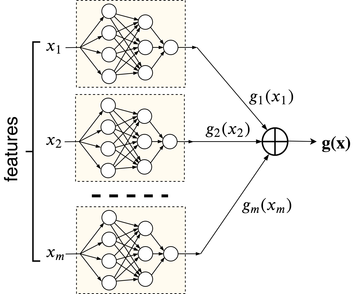
Figure 1: An illustration of NAM

GAM allows us to easily establish a partial relationships between the predicted output $y$ and the features. Moreover, the marginal impact of a single feature does not depend on the others in the model due to its additive nature. GAMs provide a better flexibility for the approximation of the black-box model and determine the feature importance by analyzing how the feature affects the predicted output through its corresponding function [73, 74].

It can be seen from Fig. 1 that NAM consists of $m$ subnetworks such that a single feature is fed to each subnetwork. Outcomes of subnetworks are values of functions $g_{i}(x_{i})$, $i=1,...,m$, which can be regarded as impacts of the corresponding features. Denote a vector of the shape functions as $\mathbf{g}(\mathbf{x})=(g_{m}(x_{m}),...,g_{m}(x_{m}))$. It should be noted that subnetworks may have different structures, but all subnetworks are trained jointly using backpropagation and can learn arbitrarily complex shape functions [14].

Suppose that the training set $D=\{(\mathbf{x}_{1},y_{1}),...,(\mathbf{x}_{n},y_{n})\}$ consists of $n$ examples, where $\mathbf{x}_{i}$ belongs to a set $\mathcal{X}\subset\mathbb{R}^{m}$ and represents a feature vector involving $m$ features, and $y_{i}\in\mathbb{R}$ represents the observed target value for regression or the class label for classification. The expected loss function $L(\mathbf{W},D)$ of the whole network can be written as follows:

$$L(\mathbf{W},D) =\sum_{i=1}^{n}l\left(y_{i},\sum_{k=1}^{m}g_{k}(x_{k}^{(i)})\right)$$

$$=\sum_{i=1}^{n}\left(y_{i}-\sum_{k=1}^{m}g_{k}(x_{k}^{(i)})\right)^{2}=\sum_{i=1}^{n}\left(y_{i}-\mathbf{g}(\mathbf{x}_{i})\cdot\mathbf{1}^{\mathrm{T}}\right)^{2},$$ (2)

where $x_{k}^{(i)}$ is the $k$-th feature of the $i$-th example; $l$ is the loss function which, for example, is the distance between the target value $y_{i}$ and the network output; $\mathbf{1}$ is the unit vector; $\mathbf{W}$ is a set of the network training parameters.

Details of the whole neural network, including its training, the used regularization techniques, activation functions, are considered in [14].

3.2 Elements of survival analysis

The training set in survival analysis consists of censored and uncensored observations. For censored observations, it is only known that the time to the event exceeds the duration of observation. The case when the time to the event coincides with the duration of the observation corresponds to the uncensored observation. Taking into account these types of observations, we can write the training set $D$ consisting of $n$ triplets $(\mathbf{x}_{i},\delta_{i},T_{i})$, $i=1,...,n$, such that $\mathbf{x}_{i}^{\mathrm{T}}=(x_{1}^{(i)},...,x_{m}^{(i)})$ is the feature vector of the $i$-th example; $T_{i}$ is the time to the event of interest; $\delta_{i}\in\{0,1\}$ is the indicator of censored or uncensored observations. In particular, $\delta_{i}=1$ when the event of interest is observed (the uncensored observation). If $\delta_{i}=0$, then we have the censored observation.

A survival machine learning model is trained on the set $D$ in order to estimate probabilistic characteristics of time $T$ to the event of interest for a new instance $\mathbf{x}$.

One of the important concepts in survival analysis is the survival function (SF) $S(t|\mathbf{x})$ which is the probability of surviving of instance $\mathbf{x}$ up to time $t$, i.e., $S(t|\mathbf{x})=\Pr\{T>t|\mathbf{x}\}$. Another important concept is the cumulative hazard function (CHF) $H(t|\mathbf{x})$, which is interpreted as the probability of an event at time $t$ given survival until time $t$. The SF $S(t|\mathbf{x})$ is determined through the CHF $H(t|\mathbf{x})$ as follows:

$$S(t|\mathbf{x})=\exp\left(-H(t|\mathbf{x})\right).$$ (3)

The CHF can also be defined as the integral of the hazard function $h(t|\mathbf{x})$ which is also used in survival analysis and defined as the rate of event at time $t$ given that no event occurred before time $t$.

An important measure characterizing a survival machine learning model, is the Harrell’s concordance index or the C-index [77]. It can be used for comparing different models and for tuning their parameters. It can be also regarded as the prediction error to evaluate the overall fitting. The C-index measures the probability that, in a randomly selected pair of examples, the example that fails first had a worst predicted outcome. It is calculated as the ratio of the number of pairs correctly ordered by the model to the total number of admissible pairs. A pair is not admissible if the events are both right-censored or if the earliest time in the pair is censored. If the C-index is equal to 1, then the corresponding survival model is supposed to be perfect. If the C-index is 0.5, then the model is not better than random guessing.

A popular regression model for the analysis of survival data is the well-known Cox proportional hazards model that calculates the effects of observed covariates on the risk of an event occurring [19]. The model assumes that the log-risk of an event of interest is a linear combination of covariates or features. This assumption is referred to as the linear proportional hazards condition. The Cox model is semi-parametric in the sense that it can be factored into a parametric part, which consists of a regression parameter vector associated with the covariates, and a non-parametric part, which can be left completely unspecified [78].

In accordance with the Cox model [19, 17], the hazard function at time $t$ given predictor values $\mathbf{x}$ is defined as

$$h(t|\mathbf{x},\mathbf{b})=h_{0}(t)\exp\left(\psi(\mathbf{x},\mathbf{b})\right).$$ (4)

Here $h_{0}(t)$ is a baseline hazard function which does not depend on the vector $\mathbf{x}$ and the vector $\mathbf{b}$; $\mathbf{b}^{\mathrm{T}}=(b_{1},...,b_{m})$ is an unknown vector of regression coefficients or parameters. The baseline hazard function represents the hazard when all of the covariates are equal to zero, i.e., it describes the hazard for zero feature vector $\mathbf{x}^{\mathrm{T}}=(0,...,0)$. The function $\psi(\mathbf{x},\mathbf{b})$ in the model is linear, i.e.,

$$\psi(\mathbf{x},\mathbf{b})=\mathbf{b}^{\mathrm{T}}\mathbf{x}=\sum\nolimits_{k=1}^{m}b_{k}x_{k}.$$ (5)

A hazard ratio is the ratio between two hazard functions $h(t|\mathbf{x}_{1},\mathbf{b})$ and $h(t|\mathbf{x}_{2},\mathbf{b})$. It is constant for the Cox model over time. In the framework of the Cox model, SF $S(t|\mathbf{x},\mathbf{b})$ is computed as

$$S(t|\mathbf{x},\mathbf{b})=\exp(-H_{0}(t)\exp\left(\psi(\mathbf{x},\mathbf{b})\right))=\left(S_{0}(t)\right)^{\exp\left(\psi(\mathbf{x},\mathbf{b})\right)}.$$ (6)

Here $H_{0}(t)$ is the baseline CHF; $S_{0}(t)$ is the baseline SF which is defined as the SF for zero feature vector $\mathbf{x}^{\mathrm{T}}=(0,...,0)$. It is important to note that functions $H_{0}(t)$ and $S_{0}(t)$ do not depend on $\mathbf{x}$ and $\mathbf{b}$.

One of the main problems of using the Cox model is linear relationship assumption between covariates and the log-risk of an event. Various modifications have been proposed to generalize the Cox model taking into account the corresponding non-linear relationship. The first group of models uses a neural network for modelling the non-linear function. Following the pioneering work of Faraggi and Simon [58], where a simple feed-forward neural network was proposed to model the non-linear relationship between covariates and the log-risk, many machine learning models have been proposed to relax this condition, including deep neural networks, the support vector machine, the random survival forest, etc. [59, 60, 79, 80, 57, 18].

One of the ways to extend the Cox model is to replace the function $\psi(\mathbf{x},\mathbf{b})$ with GAM, i.e., with the function (1). As a result, we get an extension of the Cox model with the function

$$\psi(\mathbf{x},\mathbf{g})=g_{1}(x_{1})+...+g_{m}(x_{m}).$$ (7)

The combination of GAM and the Cox model was studied by several authors [81, 12, 82].

4 An overview of the proposed main algorithm

If the have a training set $D$ and a black-box survival machine learning model trained on $D$, then the black-box model with input $\mathbf{x}$ produces the corresponding output in the form of the CHF $H(t|\mathbf{x})$ or the SF $S(t|\mathbf{x})$. The basic idea behind the explanation algorithm SurvNAM is to approximate the black-box model by the extension of the Cox model with GAM such that GAM is implemented by means of NAM trained by applying a specific loss function taking into account peculiarities of the Cox model and the black-box survival model output which is represented in the form of the SF or the CHF. In other words, we try to learn NAM for getting univariate shape functions $g_{i}$ whose sum is the function $\psi(\mathbf{x},\mathbf{g})$. For implementing the above idea, we have to define an approximation quality measure of the black-box model and the extension of the Cox model outputs and then to apply this measure to constructing the expected loss function $L(\mathbf{W},D)$ for training NAM.

Let us denote the black-box survival model output corresponding to the input vector $\mathbf{x}$ as $H(t|\mathbf{x})$ and the output of the Cox model extension as $H^{\ast}(t|\mathbf{x},\mathbf{g})$. Then the approximation quality measure mentioned above can be defined as the distance $d$ between $H(t|\mathbf{x})$ and $H^{\ast}(t|\mathbf{x},\mathbf{g})$.

Let us determine the training procedure of NAM depending on a type of explanation. If we aim to get the global explanation, then the whole dataset $D$ can be used. However, if we have to implement the local explanation for a point $\mathbf{x}$, then $N$ points $\mathbf{x}_{1},...,\mathbf{x}_{N}$ are randomly generated around $\mathbf{x}$ in accordance with a predefined probability distribution function. These examples are fed to the black-box survival model which produces a set of the corresponding CHFs $H(t|\mathbf{x}_{1}),...,H(t|\mathbf{x}_{N})$. In sum, the training set for learning NAM in the case of the local explanation is the set of the generated points and the corresponding CHFs.

A criterion of the approximation quality is the weighted mean of the distances $d$ between CHFs over all points $\mathbf{x}_{1},...,\mathbf{x}_{N}$ where each weight depends on the distance between generated point $\mathbf{x}_{k}$ and explained point $\mathbf{x}$. Smaller distances between $\mathbf{x}_{k}$ and $\mathbf{x}$ produce larger weights of distances between CHFs.

In fact, we have a double approximation. First, we implicitly approximate the black-box survival model by the extended Cox model. This approximation is implicit because its result is the loss function taking into account the distance between the black-box survival model prediction and the extended Cox model prediction. Second, we learn the neural network (NAM) to find shape functions approximating the extended Cox model.

A general scheme of SurvNAM is shown in Fig. 2. The black-box survival model is trained on $N$ vectors of training examples such that each example consists of $m$ features. Predictions of the model are CHFs. In accordance with the Cox model, the baseline CHF is estimated, and the predictions of the extended Cox models are represented as functions of the training vectors $\mathbf{x}_{i}$ and the vector of shape functions $\mathbf{g}(\mathbf{x}_{i})$. The weighted average distance between predictions of the black-box survival model and the prediction representation of the extended Cox model compose the loss function for training NAM. By having the trained NAM, we get shape functions $g_{1}(x_{1}),...,g_{m}(x_{m})$ for all features. These functions can be viewed as explanation of the predictions and the corresponding survival model.

Figure 2: A schematic illustration of SurvNAM

5 The expected loss function

The loss function for training NAM differs from the standard loss function like (2). First, it has to take into account the peculiarity of the black-box survival model output which is a function (the CHF or the SF). Second, it has to take into account peculiarities of the Cox model extension. Third, the loss function should be convex to get optimal solution.

Before deriving the loss function, we introduce some notations and conditions.

Let $t_{0}<t_{1}<...<t_{s}$ be distinct times to events of interest, for example, times to the patient deaths from the set $\{T_{1},...,T_{n}\}$, where $t_{0}=\min_{k=1,...,n}T_{k}$ and $t_{s}=\max_{k=1,...,n}T_{k}$. The black-box model maps the feature vectors $\mathbf{x}\in\mathbb{R}^{m}$ into piecewise constant CHFs $H(t|\mathbf{x})$. It is assumed that $\max_{t}H(t|\mathbf{x})<\infty$.

Let us introduce the time $T=t_{s}+\gamma$ in order to restrict the integral of $H(t|\mathbf{x})$, where $\gamma$ is a small positive number. Let $\Omega=[0,T]$. Then we can write $\int_{\Omega}H(t|\mathbf{x})\mathrm{d}t<\infty$. Since the CHF $H(t|\mathbf{x})$ is piecewise constant, then it can be written in a special form. Let us divide the set $\Omega$ into $s+1$ subsets $\Omega_{0},...,\Omega_{s}$ such that $\Omega=\cup_{j=0,...,s}\Omega_{j}$, where $\Omega_{s}=[t_{s},T]$, $\Omega_{j}=[t_{j},t_{j+1})$, $\forall j\in\{0,...,s-1\}$, and $\Omega_{j}\cap\Omega_{k}=\emptyset$ for $\forall j\neq k$

The CHF $H(t|\mathbf{x})$ can be expressed through the indicator functions as follows:

$$H(t|\mathbf{x})=\sum_{j=0}^{s}H_{j}(\mathbf{x})\cdot\chi_{\Omega_{j}}(t),$$ (8)

where $\chi_{\Omega_{j}}(t)$ is the indicator function taking value $1$ if $t\in\Omega_{j}$, and $0$ otherwise; $H_{j}(\mathbf{x})$ is a part of the CHF in interval $\Omega_{j}$, which is constant in $\Omega_{j}$ and does not depend on $t$.

Let us write similar expressions for the CHF of the Cox model extension:

$$H^{\ast}(t|\mathbf{x},\mathbf{g})=H_{0}(t)\exp\left(\psi(\mathbf{x},\mathbf{g})\right)=\sum_{j=0}^{s}\left[H_{0j}\exp\left(\psi(\mathbf{x},\mathbf{g})\right)\right]\chi_{\Omega_{j}}(t).$$ (9)

By having the above expressions for the $H(t|\mathbf{x})$ and $H^{\ast}(t|\mathbf{x},\mathbf{g})$, we can construct the loss function as the weighted Euclidean distance between $H(t|\mathbf{x}_{i})$ and $H^{\ast}(t|\mathbf{x}_{i},\mathbf{g}_{i})$ for all generated $\mathbf{x}_{i}$, $i=1,...,N$:

$$L(\mathbf{W},D)=\sum_{i=1}^{N}v_{i}\int_{\Omega}\left\|H(t|\mathbf{x}_{i})-H^{\ast}(t|\mathbf{x}_{i},\mathbf{g}_{i})\right\|_{2}^{2}\mathrm{d}t,$$

where the integral is taken over the set $\Omega$ because we define the distance between functions of time $t$; $v_{i}$ is the weight depending on the distance between generated point $\mathbf{x}_{i}$ and explained point $\mathbf{x}$; $\mathbf{x}_{i}$ is the generated point.

Since the CHFs are represented as piecewise constant function of the form (8) and (9), then it is simply to prove that the integral in the loss function can be replaced by the sum as follows:

$$L(\mathbf{W},D)=\sum_{i=1}^{N}v_{i}\sum_{j=0}^{s}\left(H_{j}(\mathbf{x}_{i})-\left[H_{0j}\exp\psi(\mathbf{x}_{i},\mathbf{g}_{i})\right]\right)^{2}\tau_{j}.$$ (10)

where $\tau_{j}=t_{j+1}-t_{j}$.

The main difficulty of using the CHFs is that the loss function $L(\mathbf{W},D)$ may be non-convex. Therefore, we replace CHFs with their logarithms and find distances between logarithms of CHFs. Since the logarithm is a monotone function, then there holds:

$$L(\mathbf{W},D)=\sum_{i=1}^{N}v_{i}\sum_{j=0}^{s}\left(\ln H_{j}(\mathbf{x}_{i})-\ln H_{0j}-\psi(\mathbf{x}_{i},\mathbf{g}_{i})\right)^{2}\tau_{j}.$$ (11)

Let us introduce the following notation for short:

$$\Phi_{j}(\mathbf{x}_{i})=\ln H_{j}(\mathbf{x}_{i})-\ln H_{0j}.$$ (12)

Hence, we get the final expected loss function

$$L(\mathbf{W},D)=\sum_{i=1}^{N}v_{i}\sum_{j=0}^{s}\left(\Phi_{j}(\mathbf{x}_{i})-\sum_{k=1}^{m}g_{k}(x_{k}^{(i)})\right)^{2}\tau_{j}.$$ (13)

Parameters $\mathbf{W}$ of the neural network are implicitly contained in calculating functions $g_{k}$. By adding the regularization term to the loss function (13), we get

$$L(\mathbf{W},D)=\sum_{i=1}^{N}v_{i}\sum_{j=0}^{s}\left(\Phi_{j}(\mathbf{x}_{i})-\sum_{k=1}^{m}g_{k}(x_{k}^{(i)})\right)^{2}\tau_{j}.$$

We also assume that $H_{j}(\mathbf{x})\geq\varepsilon>0$ for all $\mathbf{x}$ in order to avoid the case when the logarithm of zero is calculated. It should be noted that the loss function (11) is not equivalent to the previous loss function (10). However, this is not so important because we train the neural network which is fitted to the changed loss function. Since $\psi(\mathbf{x}_{i},\mathbf{g}_{i})$ is the sum of the functions $\mathbf{g}_{i}$ which are outputs of NAM, then $\ln H_{j}(\mathbf{x}_{i})-\ln H_{0j}-\sum_{k=1}^{m}g_{k}(x_{k}^{(i)})$ in (13) is the linear function of shape functions $g_{k}(x_{k}^{(i)})$. It follows from the above and from positivity of $\tau_{j}$ and $v_{i}$ that the expected loss function (13) is convex. The weight $v_{i}$ is taken as a decreasing function of the distance between $\mathbf{x}$ and $\mathbf{x}_{i}$, for example, $v_{k}=K(\mathbf{x},\mathbf{x}_{k})$, where $K(\cdot,\cdot)$ is a kernel.

In sum, we have the expected convex loss function (13) for training NAM, which can be written as

$$L(\mathbf{W},D)=\sum_{i=1}^{N}\sum_{j=0}^{s}\left(\sqrt{v_{i}\tau_{j}}\Phi_{j}(\mathbf{x}_{i})-\sqrt{v_{i}\tau_{j}}\sum_{k=1}^{m}g_{k}(x_{k}^{(i)})\right)^{2}.$$

6 Lasso-based modifications of SurvNAM for the local explanation

The main difficulty of the proposed approach is that neural subnetworks computing shape functions $g_{k}$, $k=1,...,m$, may be overfitted due to the noise from unimportant features. As a result, the approximation may be unsatisfactory, and important features may be incorrectly ranked. In order to overcome this difficulty, a sparse modification of SurvNAM is proposed by using the Lasso method or the $L_{1}$-norm for regularization.

Let us write the GAM as follows:

$$g(\mathbb{E}(y(\mathbf{x}))=\beta_{1}g_{1}(x_{1})+...+\beta_{m}g_{m}(x_{m}),$$ (14)

where $\beta_{k}\in\mathbb{R}$ is a coefficient.

It is assumed here that the $k$-th shape function $g_{k}$ has some coefficient $\beta_{k}$ which determines the impact of function $g_{k}$ on the prediction. The constraint that $\mathbf{\beta}$ lies in the $L_{1}$-ball encourages sparsity of the estimated $\mathbf{\beta}$ [83]. This implies that if we add the regularization term $\left\|\mathbf{\beta}\right\|_{1}=\sum_{k=1}^{m}\left|\beta_{k}\right|$, then we can expect that a part of coefficients $\beta_{k}$, corresponding to unimportant features, will be $0$ or close to $0$ due to properties of the regularization. Hence, the neural subnetworks, corresponding to unimportant features, will not introduce the additional noise to results. It should be noted that the sparse GAM has been studied by several authors [84, 85, 83].

The loss function (13) for training the neural network can be rewritten in accordance with the idea of using the regularization term $\left\|\mathbf{\beta}\right\|_{1}$ as follows:

$$L(\mathbf{W},D) =\sum_{i=1}^{N}v_{i}\sum_{j=0}^{s}\left(\Phi_{j}(\mathbf{x}_{i})-\sum_{k=1}^{m}\beta_{k}g_{k}(x_{k}^{(i)})\right)^{2}\tau_{j}$$

$$+\lambda\sum_{k=1}^{m}\left|\beta_{k}\right|,$$ (15)

where $\lambda$ is a hyper-parameter which controls the strength of the regularization.

In fact, every neural subnetwork is assigned by the weight $\beta_{k}$. It should be pointed out that the use of the $L_{1}$-norm as the regularization term in SurvNAM for the sparse explanation differs from use of the original Lasso method. We use functions $g_{k}$ instead of variables $x_{k}$ here, which can generally be non-linear. It should be also pointed out that the visual analysis of shape functions $g_{k}$ is replaced with the analysis of functions $\beta_{k}g_{k}$, $k=1,...,m$. Numerical experiments with the above modification of SurvNAM show that the main difficulty of its use is that the functions $g_{k}(x_{k}^{(i)})$ may increase in order to balance small values of $\beta_{k}$. A simple way to overcome this difficulty is to restrict the set of possible functions $g_{k}$. Since function $g_{k}$ is represented as some function implemented by the $k$-th subnetwork, then its restriction depends on weights of the subnetwork. Therefore, the set of functions $g_{k}$ can be restricted by regularizing all weights $w_{i}$ of the network connections. Hence, we add the term $\mu\left\|\mathbf{W}\right\|_{2}^{2}$ to the loss function, where $\left\|\mathbf{W}\right\|_{2}^{2}$ is the short notation of the squared $L_{2}$-norm for all training parameters $w_{i}$ of the neural network, $\mu$ is a hyper-parameter which controls the strength of the regularization.

Another modification is based on the idea to add a linear component to each function $g_{k}$, i.e., we replace the product $\beta_{k}g_{k}(x_{k}^{(i)})$ with the sum $\alpha_{k}g_{k}(x_{k}^{(i)})+(1-\alpha_{k})\omega_{k}x_{k}^{(i)}$. This is an interesting idea because it formally relates to the shortcut connection in the well-known ResNet proposed by He et al. [86]. This connection is skipping one or more layers in the neural network. It plays an important role in alleviating the vanishing gradient problem [87]. The shortcut connection with regard to the $k$-th neural subnetwork in the modification of SurvNAM is depicted in Fig. 3.

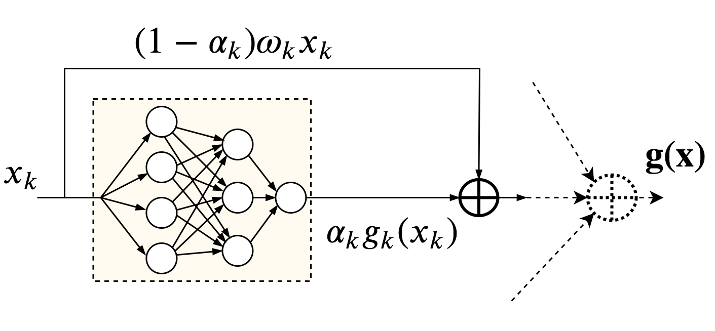
Figure 3: The shortcut connection with regard to the modification of SurvNAM

The aforementioned relationship between the proposed modification of SurvNAM and the ResNet is very surprising. The difference is that the shortcut connection in SurvNAM has the weight $(1-\alpha_{k})\omega_{k}$ which consists of two training parameters $\alpha_{k}$ and $\omega_{k}$. The parameter $\alpha_{k}$ can be viewed as a measure of the $k$-th feature contribution non-linearity. The term $(1-\alpha_{k})$ is a measure of the $k$-th feature contribution linearity. The greater the value of $(1-\alpha_{k})$, the greater linearity of the $k$-th feature and the smaller the impact of $g_{k}$. An idea behind the use of parameter $\omega_{k}$ is based on the following reasoning. Parameter $\alpha_{k}$ chooses between the subnetwork (function $g_{k}$) and the linear function $x_{k}$. Therefore, $\alpha_{k}$ cannot play a role of an angle of inclination of the line $x_{k}$. This implies that we add parameter $\omega_{k}$ to take into account this angle. In other words, we can represent the sum $\alpha_{k}g_{k}(x_{k})+(1-\alpha_{k})\omega_{k}x_{k}$ as $\alpha_{k}g_{k}(x_{k})+(1-\alpha_{k})r_{k}$, where $r_{k}=\omega_{k}x_{k}$.

Taking into account restrictions for the network parameters in the form of the $L_{2}$ regularization $\left\|\mathbf{W}\right\|_{2}^{2}$, we write the loss function for training the whole neural network as follows:

$$L(\mathbf{W},D) =\sum_{i=1}^{N}v_{i}\sum_{j=0}^{s}\left(\Phi_{j}(\mathbf{x}_{i})-\sum_{k=1}^{m}\alpha_{k}g_{k}(x_{k}^{(i)})-\sum_{k=1}^{m}(1-\alpha_{k})\omega_{k}x_{k}^{(i)}\right)^{2}\tau_{j}$$

$$+\lambda\sum_{k=1}^{m}\left|\alpha_{k}\right|+\mu\cdot\left\|\mathbf{W}\right\|_{2}^{2}.$$ (16)

In contrast to the ResNet, the shortcut connection in SurvNAM plays a double role. First, it alleviates the vanishing gradient problem when the network is training. Second, it allows us to see how the linear part of the shape function impacts on the prediction.

7 Numerical experiments

SurvNAM is tested on five real benchmark datasets. A short introduction of the benchmark datasets are given below.

The German Breast Cancer Study Group 2 (GBSG2) Dataset contains observations of 686 women. Every example is characterized by 10 features, including age of the patients in years, menopausal status, tumor size, tumor grade, number of positive nodes, hormonal therapy, progesterone receptor, estrogen receptor, recurrence free survival time, censoring indicator (0 - censored, 1 - event). The dataset can be obtained via the “TH.data” R package.

The Monoclonal Gammopathy (MGUS2) Dataset contains the natural history of 1384 subjects with monoclonal gammopathy of undetermined significance characterized by 5 features. The dataset can be obtained via the “survival” R package.

The Survival from Malignant Melanoma (Melanoma) Dataset consist of measurements made on patients with malignant melanoma. The dataset contains data on 205 patients characterized by 7 features. The dataset can be obtained via the “boot” R package.

The Stanford Heart Transplant (Stanford2) Dataset contains data on survival of 185 patients on the waiting list for the Stanford heart transplant program. The dataset can be obtained via the “survival” R package.

The Veterans’ Administration Lung Cancer Study (Veteran) Dataset contains data on 137 males with advanced inoperable lung cancer. The subjects were randomly assigned to either a standard chemotherapy treatment or a test chemotherapy treatment. Several additional variables were also measured on the subjects. The dataset can be obtained via the “survival” R package.

For the local explanation, the perturbation technique is used. In accordance with the technique, $N$ nearest points $\mathbf{x}_{k}$ are generated in a local area around the explained example $\mathbf{x}$. These points are normally distributed with the center at point $\mathbf{x}$ and the standard deviation which is equal to $10\%$ of the largest distance between points of the corresponding studied dataset. In numerical experiments, $N=100$. The weight to the $k$-th point $\mathbf{x}_{k}$ is assigned as follows:

$$w_{k}=1-\sqrt{\frac{\left\|\mathbf{x}-\mathbf{x}_{k}\right\|_{2}}{r}},\ k=1,...,N.$$ (17)

As a black-box model, we use the RSF model [63] consisting of $500$ decision survival trees. The approximating Cox model has the baseline CHF $H_{0}(t)$ constructed on training data using the Nelson–Aalen estimator.

The Python code of NAM is taken from https://github.com/google-research/google-research/tree/master/neural_additive_models. It is modified to implement the proposed methods.

7.1 Numerical experiments with SurvNAM

First, we test SurvNAM trained on the GBSG2 dataset for the local explanation. Fig. 4 illustrates SFs obtained by means of the RSF for $6$ randomly selected examples from the training set (the right picture) and by means of the extended Cox model with the shape functions $g_{i}(x_{i})$ of the GAM provided by SurvNAM (the left picture). SFs shown in the left picture of Fig. 4 can be viewed as approximations approximating of the corresponding SFs depicted in the right picture. The same CHFs obtained by the RSF (the right picture) and by the extended Cox model (the left picture) are shown in Fig. 5. Shape functions for all features are illustrated in Fig. 6. They are computed for an example with features “age”=44, “estrec”=67, “horTh”=yes, “menostat”=Post, “pnodes”=6, “progrec”=150, “tsize”=20, “tgrade”=1. Every picture in Fig. 6 shows how a separate feature contributes into the prediction. Color vertical bars in every picture represent the normalized data density for each feature. Only numerical features are considered for the local explanation. It can be seen from Fig. 6 that the feature “pnodes” (the number of positive nodes) is the most important especially when its value is larger than $2$. This conclusion follows from the fact that the corresponding shape function significantly increases.

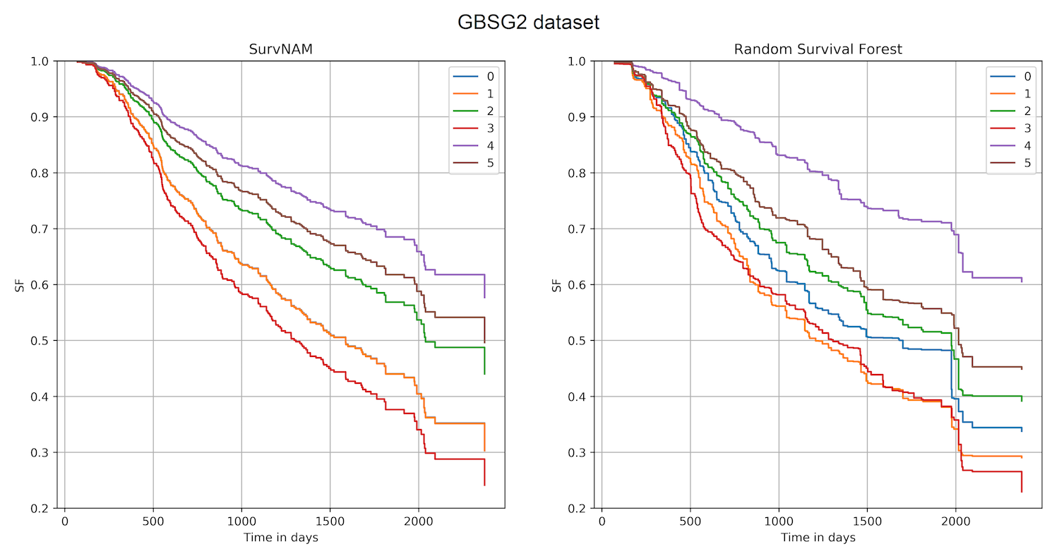
Figure 4: SFs obtained by means of SurvNAM (left picture) and the black-box RSF model (right picture) for the dataset GBSG2 and the local explanation

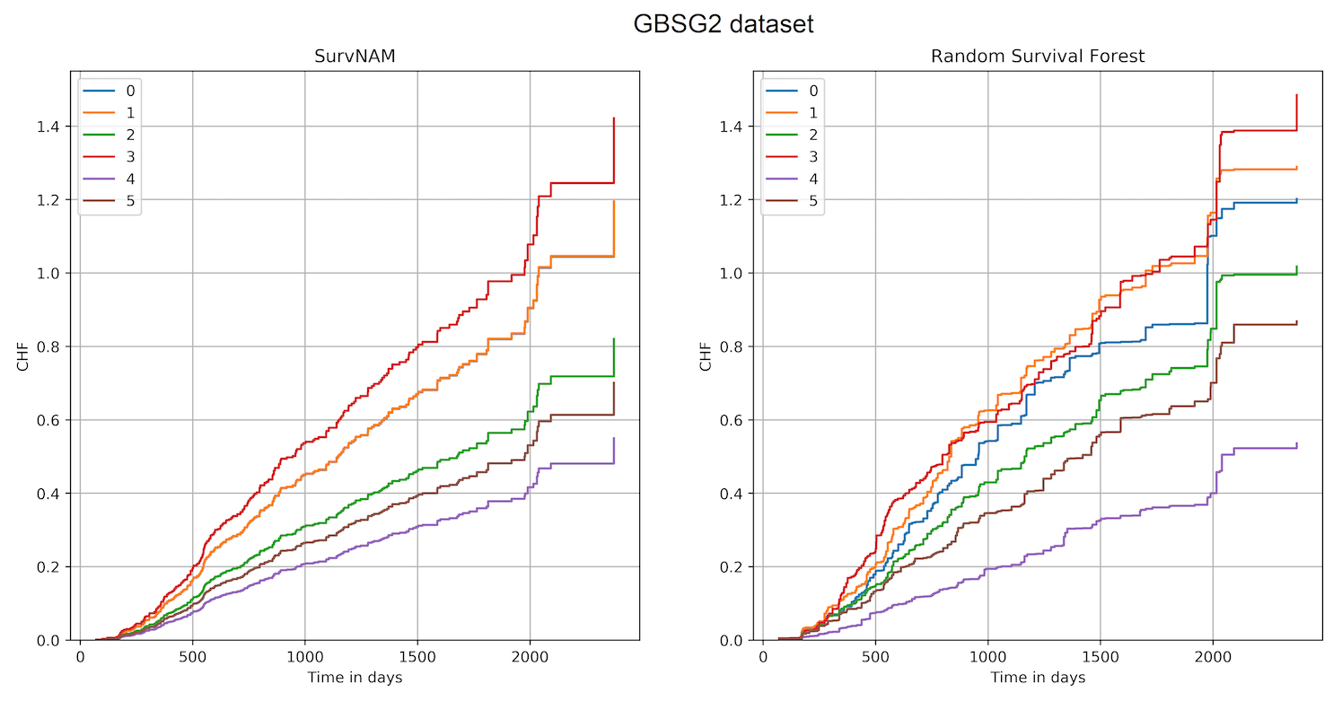
Figure 5: CHFs obtained by means of SurvNAM (left picture) and the black-box RSF model (right picture) for the dataset GBSG2 and the local explanation

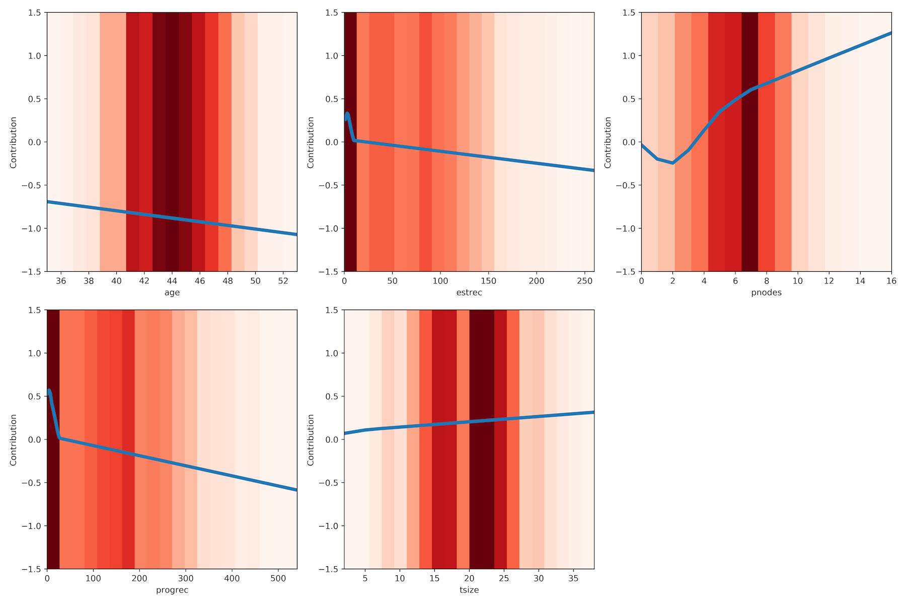
Figure 6: Shape functions for every feature obtained by means of SurvNAM for the dataset GBSG2 and the local explanation

Let us consider how SurvNAM behaves for the case of the global explanation when it is trained on the GBSG2 dataset. The shape functions for all features are illustrated in Fig. 7. One can again see from Fig. 7 that the number of positive nodes (“pnodes”) is the most important feature. On the one hand, features “progrec” (progesterone receptor) and “tsize” (tumor size) can be also regarded as important ones. On the other hand, if we look at the normalized data density (color bar), then feature “age” becomes also important the main part of its shape function is changed for a larger number of examples in comparison, for example, with feature “progrec”. In a whole, one can observe from Figs. 6 and 7 that tendency of the feature value changes are similar for local and global explanations.

The RSF is characterized by the C-index equal to $0.676$. The C-index of SurvNAM is $0.687$. The C-indices are computed on test data.

For comparison purposes, we also apply the well-known permutation feature importance method [88]. The largest importance values indicate the top three features which are “pnodes”, “progrec”, and “age” with the importance values $0.083$, $0.057$, $0.023$, respectively.

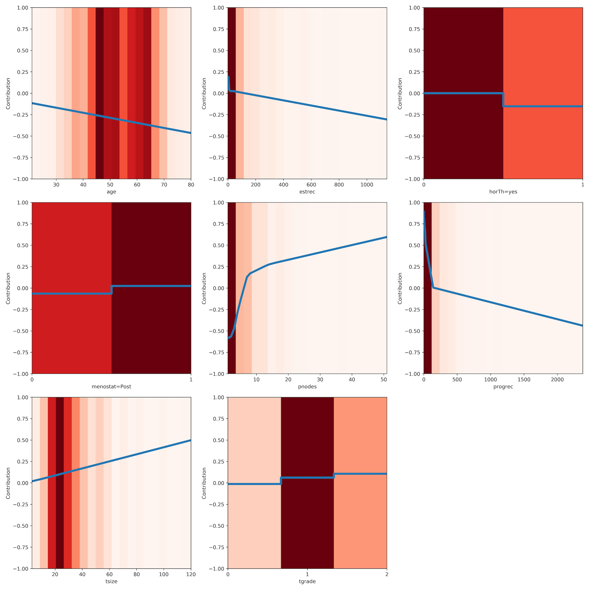
Figure 7: Shape functions for every feature obtained by means of SurvNAM for the dataset GBSG2 and the global explanation

Another dataset for illustrating SurvNAM is the MGUS2 dataset. Figs. 8 and 9 show SFs and CHFs obtained by means of the RSF for $6$ randomly selected examples from the training set (the right picture) and by means of the extended Cox model with the shape functions $g_{i}(x_{i})$ of the GAM provided by SurvNAM (the left picture). The pictures are similar to the corresponding pictures given in Figs. 4 and 5. It can be seen from Figs. 8 and 9 that the SurvNAM predictions are weakly approximate the RSF output. Two possible reasons can be adduced to explain the above disagreement. First, the baseline CHF $H_{0}(t)$ may be unsatisfactory determined when the dataset is significantly heterogeneous. Second, features are strongly correlated, and it is difficult to construct the GAM for its using in the Cox model.

Shape functions for all features are illustrated in Fig. 10. They are computed for an example with features “age”=65, “sex”=M, “hgb”=13.5, “creat”=2.4, “mspike”=1.5. It can be seen from Fig. 10 that the feature “creat” (creatinine) is the most important. The feature “age” (age at diagnosis) can be also regarded as important.

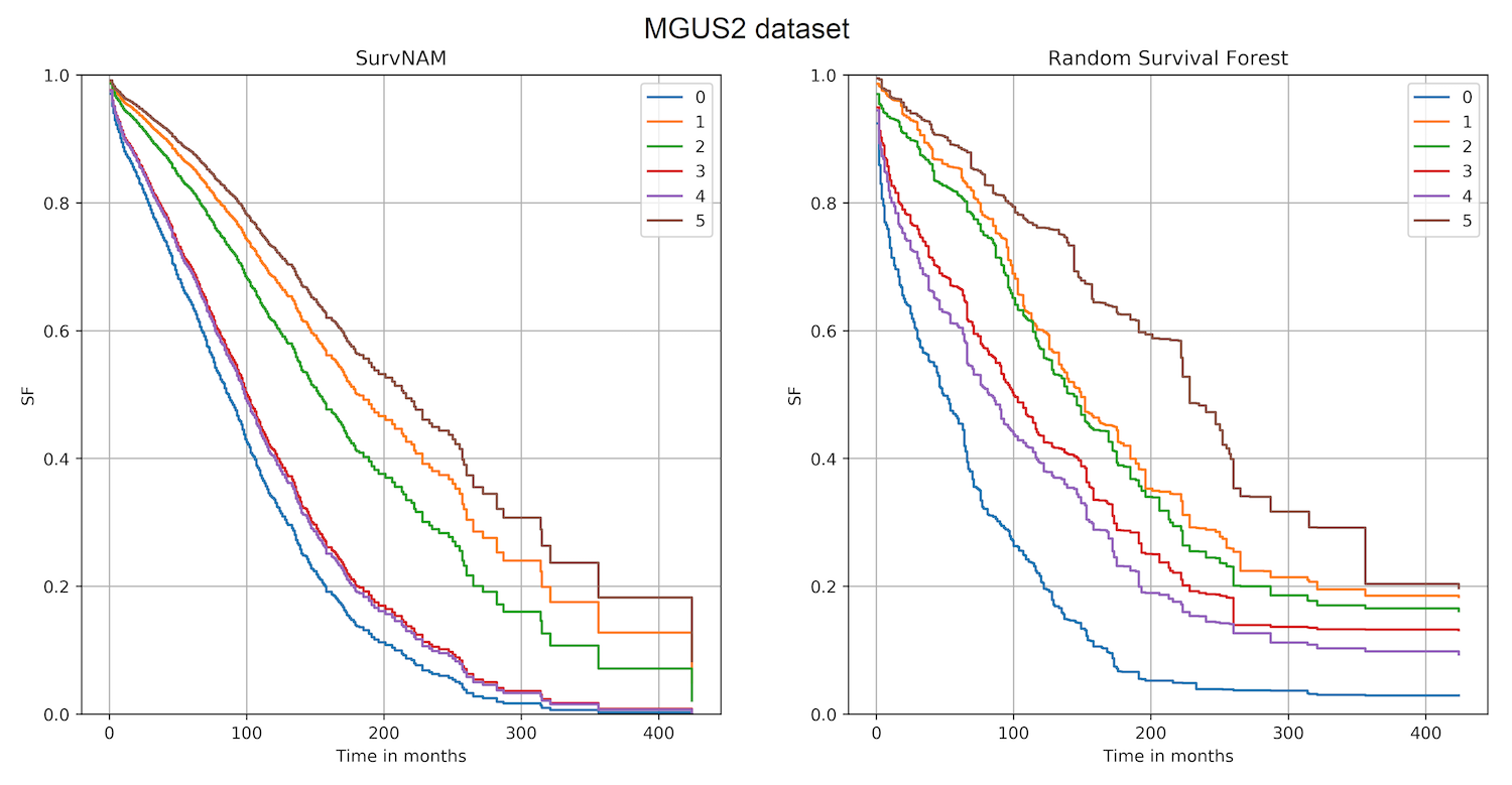
Figure 8: SFs obtained by means of SurvNAM (left picture) and the black-box RSF model (right picture) for the dataset MGUS2 and the local explanation

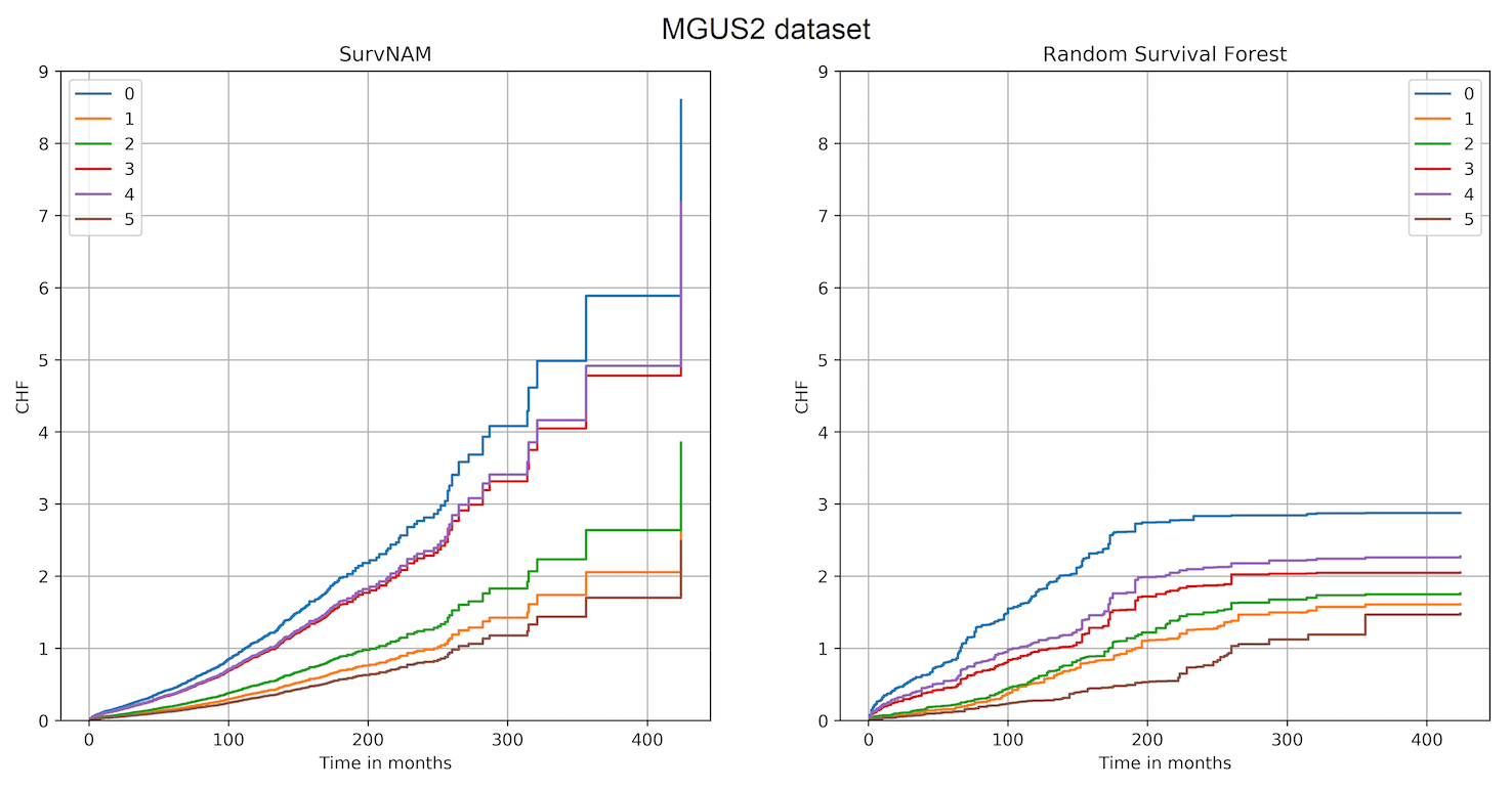
Figure 9: CHFs obtained by means of SurvNAM (left picture) and the black-box RSF model (right picture) for the dataset MGUS2 and the local explanation

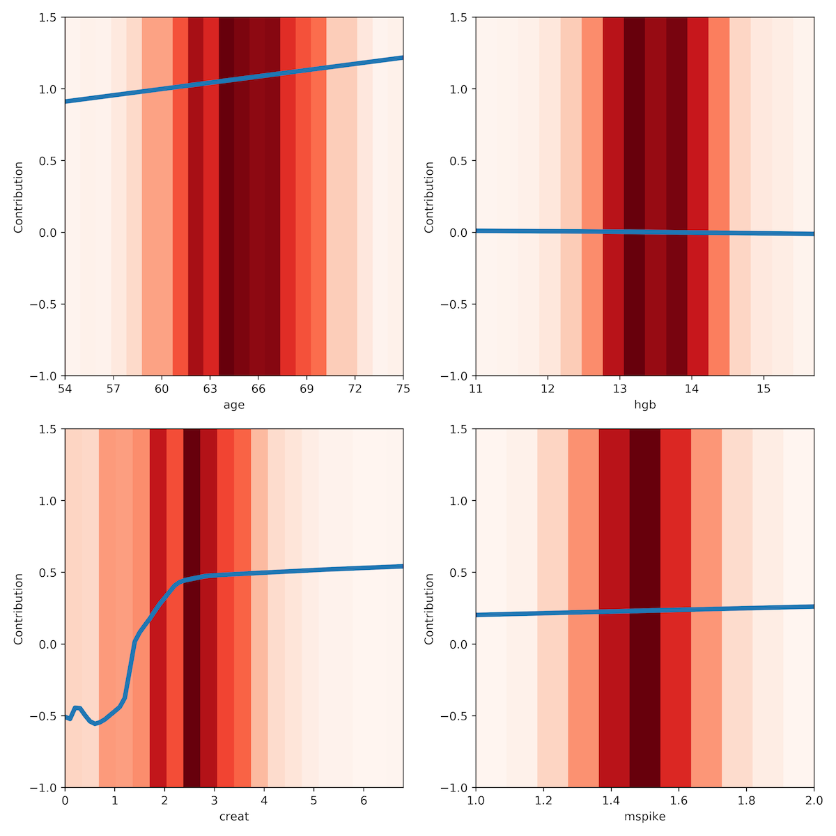
Figure 10: Shape functions for every feature obtained by means of SurvNAM for the dataset MGUS2 and the local explanation

The shape functions for the global explanation are illustrated in Fig. 11. It can be seen from Fig. 11 that “age” and “hgb” are the most important features. This conforms with results provided by the permutation feature importance method. According to this method, the top three features are “age”, “hgb”, and “creat” with the importance values $0.193$, $0.041$, $0.027$, respectively.

The RSF is characterized by the C-index equal to $0.687$. The C-index of SurvNAM is $0.691$. The C-indices are computed on test data.

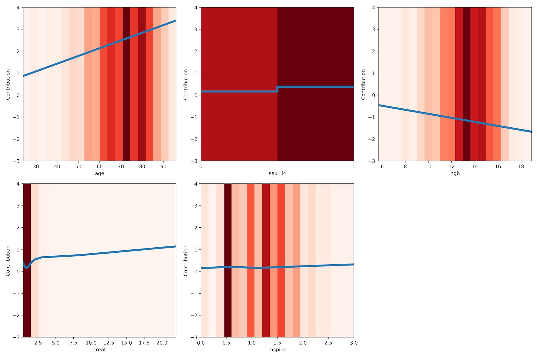
Figure 11: Shape functions for every feature obtained by means of SurvNAM for the dataset MGUS2 and the global explanation

Let us consider the Melanoma dataset. Figs. 12 and 13 show SFs and CHFs obtained by means of the RSF for $6$ randomly selected examples from the training set (the right picture) and by means of the extended Cox model with the shape functions $g_{i}(x_{i})$ of the GAM provided by SurvNAM (the left picture). In contrast to the MGUS2 dataset, SFs and CHFs provided by the RSF and SurvNAM are close to each other. Shape functions for all features are illustrated in Fig. 14. They are computed for an example with features “sex”=M, “age”=53, “thickness”=1.62, “ulcer”=present. It can be seen from Fig. 14 that the feature “thickness” (the tumor thickness) is the most important.

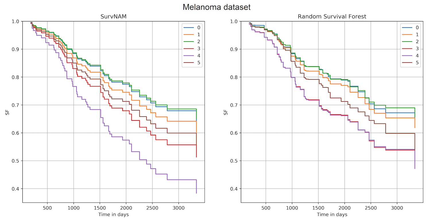
Figure 12: SFs obtained by means of SurvNAM (left picture) and the black-box RSF model (right picture) for the dataset Melanoma and the local explanation

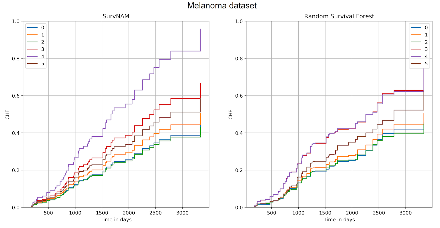
Figure 13: CHFs obtained by means of SurvNAM (left picture) and the black-box RSF model (right picture) for the dataset Melanoma and the local explanation

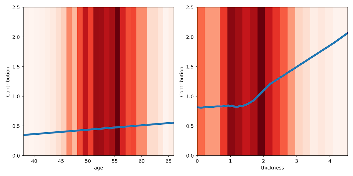
Figure 14: Shape functions for every feature obtained by means of SurvNAM for the dataset Melanoma and the local explanation

The shape functions for the global explanation are illustrated in Fig. 15. It can be seen from Fig. 15 that “thickness” and “ulcer” are the most important features. The above result conforms with results provided by the permutation feature importance method. According to this method, the top three features are “thickness”, “ulcer”, and “age” with the importance values $0.189$, $0.033$, $0.026$, respectively. The importance values justify “thickness” and “ulcer” as the most important features. The RSF is characterized by the C-index equal to $0.779$. The C-index of SurvNAM is $0.788$. The C-indices are computed on test data.

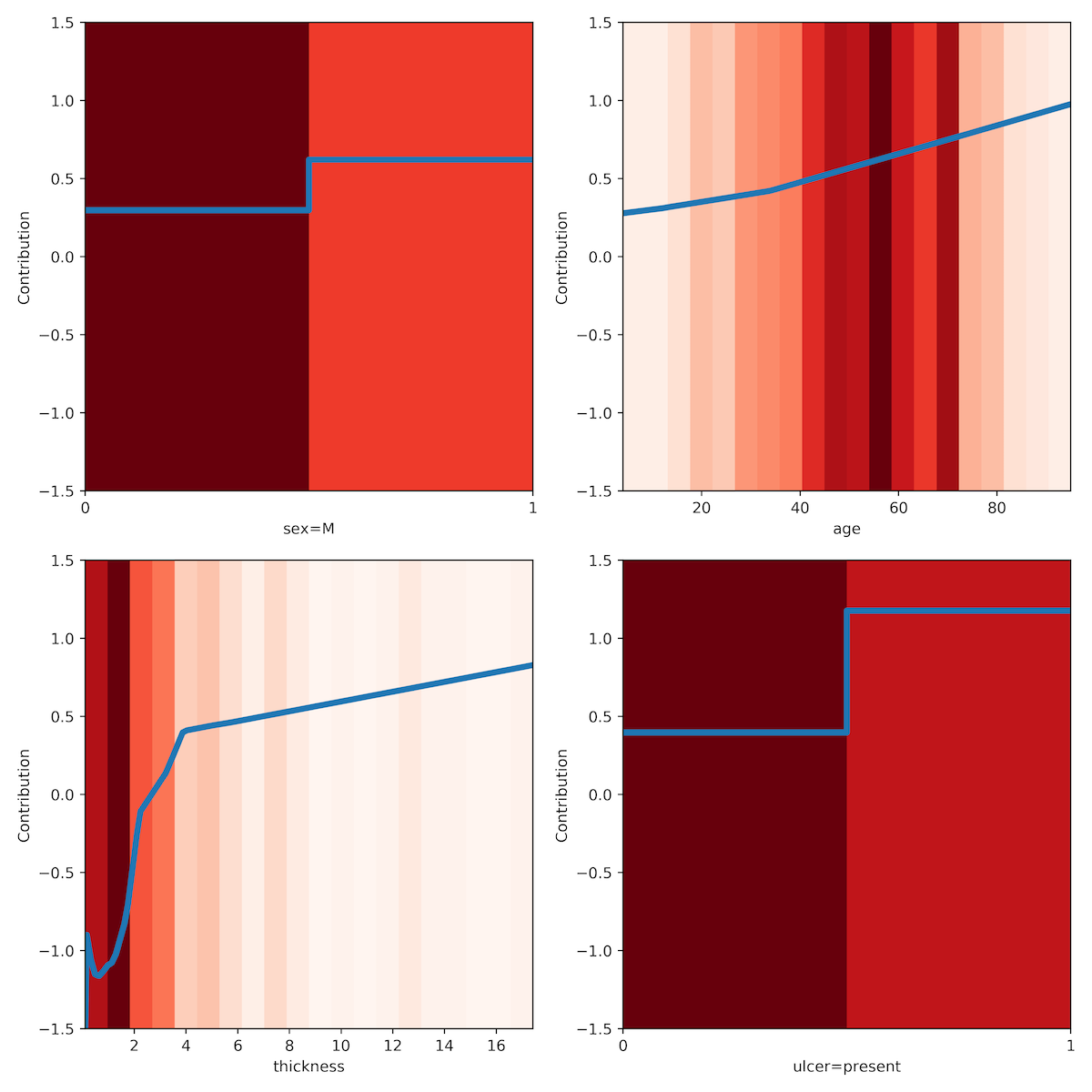
Figure 15: Shape functions for every feature obtained by means of SurvNAM for the dataset Melanoma and the global explanation

The next dataset is Stanford2. Figs. 16 and 17 show SFs and CHFs obtained by means of the RSF for $6$ randomly selected examples from the training set (the right picture) and by means of the extended Cox model with the shape functions $g_{i}(x_{i})$ of the GAM provided by SurvNAM (the left picture). In contrast to the Stanford2 dataset, SFs and CHFs provided by the RSF and SurvNAM are close to each other. Shape functions for the local explanation are illustrated in Fig. 18. They are computed for an example with features “age”=42, “t5”=1.74. It can be seen from Fig. 18 that the feature “age” is the most important. The same can be concluded for the global explanation (see Fig. 19).

This result conforms with results provided by the permutation feature importance method. According to this method, the important feature is “age” with the importance value $0.127$. The importance value of “t5” is $0.068$. The RSF is characterized by the C-index equal to $0.643$. The C-index of SurvNAM is $0.669$. The C-indices are computed on test data.

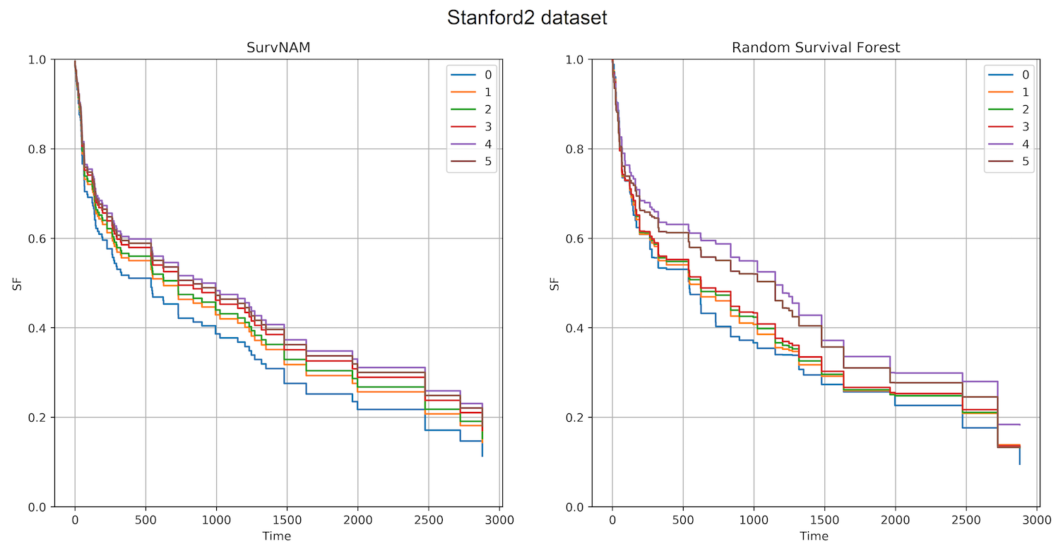
Figure 16: SFs obtained by means of SurvNAM (left picture) and the black-box RSF model (right picture) for the dataset Stanford2 and the local explanation

Figure 17: CHFs obtained by means of SurvNAM (left picture) and the black-box RSF model (right picture) for the dataset Stanford2 and the local explanation

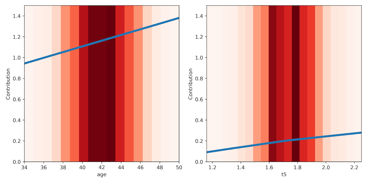
Figure 18: Shape functions for every feature obtained by means of SurvNAM for the dataset Stanford2 and the local explanation

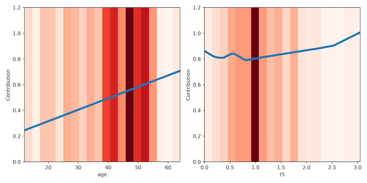
Figure 19: Shape functions for every feature obtained by means of SurvNAM for the dataset Stanford2 and the global explanation

Let us investigate SurvNAM by taking the well-known Veteran dataset. Examples of the dataset Veteran consist of most categorical features. Therefore, we consider only the global explanation for this dataset. The shape functions are illustrated in Fig. 20. It can be seen from Fig. 20 that “Karnofsky score” and “Celltype squamous” are the most important features. According to the permutation feature importance method, the top three features are “Karnofsky score”, “Celltype smallcell”, and “Celltype squamous” with the importance values $0.163$, $0.020$, $0.008$, respectively. The above results do not totally conform with results provided by SurvNAM. We can see from SurvNAM that “Celltype squamous” is more important in comparison with “Celltype smallcell”.

The RSF is characterized by the C-index equal to $0.725$. The C-index of SurvNAM is $0.731$. The C-indices are computed on test data.

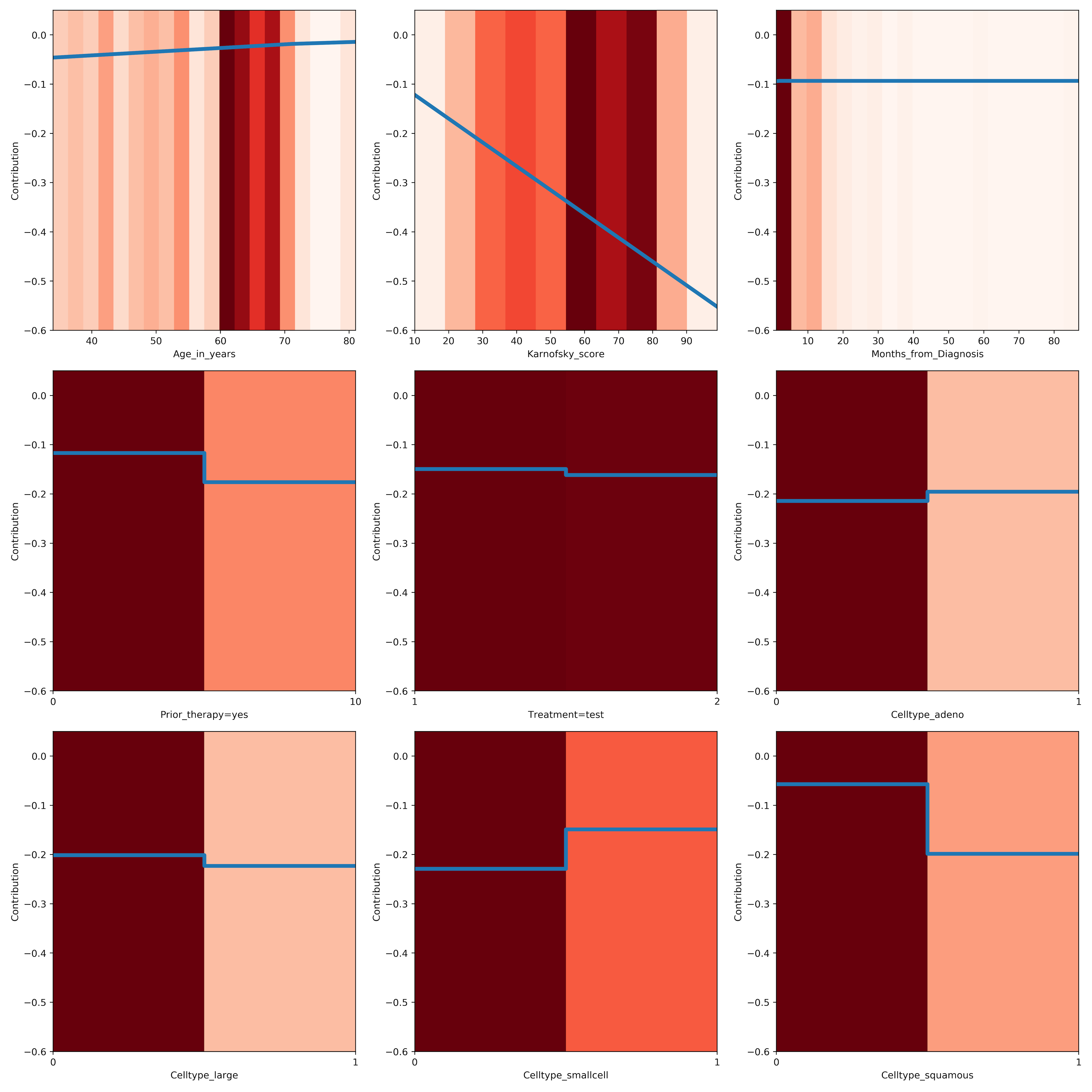
Figure 20: Shape functions for every feature obtained by means of SurvNAM for the dataset Veteran and the global explanation

7.2 Numerical experiments with modifications of SurvNAM

Let us consider how modifications of SurvNAM impact on the shape functions of features.

First, we study the dataset GBSG2 for the local explanation. It can be seen from Fig. 6 that feature “pnodes” (the third picture in the first row) has an unexplainable interval of decreasing when the feature values are in the interval from $0$ to $2$. It is difficult to expect that the contribution to the recurrence free survival time is reduced when the number of positive nodes is $2$. One of the reasons of this behavior of the shape function is the network overfitting. The same can be said about small values of features “estrec” (estrogen receptor) and “progrec” (progesterone receptor) (see Fig. 6). Let us apply the first modification of SurvNAM and train the network in accordance with the loss function (15). The corresponding shape functions of analyzed features are depicted in Fig. 21. Results in Fig. 21 are obtained under condition that hyperparameter $\lambda$ controlling the strength of constraints for parameters $\beta$ in (15) is $10$. It should be noted that $\lambda=1$ does not impact on the shape functions. On the other hand, the case $\lambda=100$ significantly reduces the approximation accuracy of the extended Cox model and the black-box model. One can see from Fig. 21 that the first modification only partly solves the network overfitting problem.

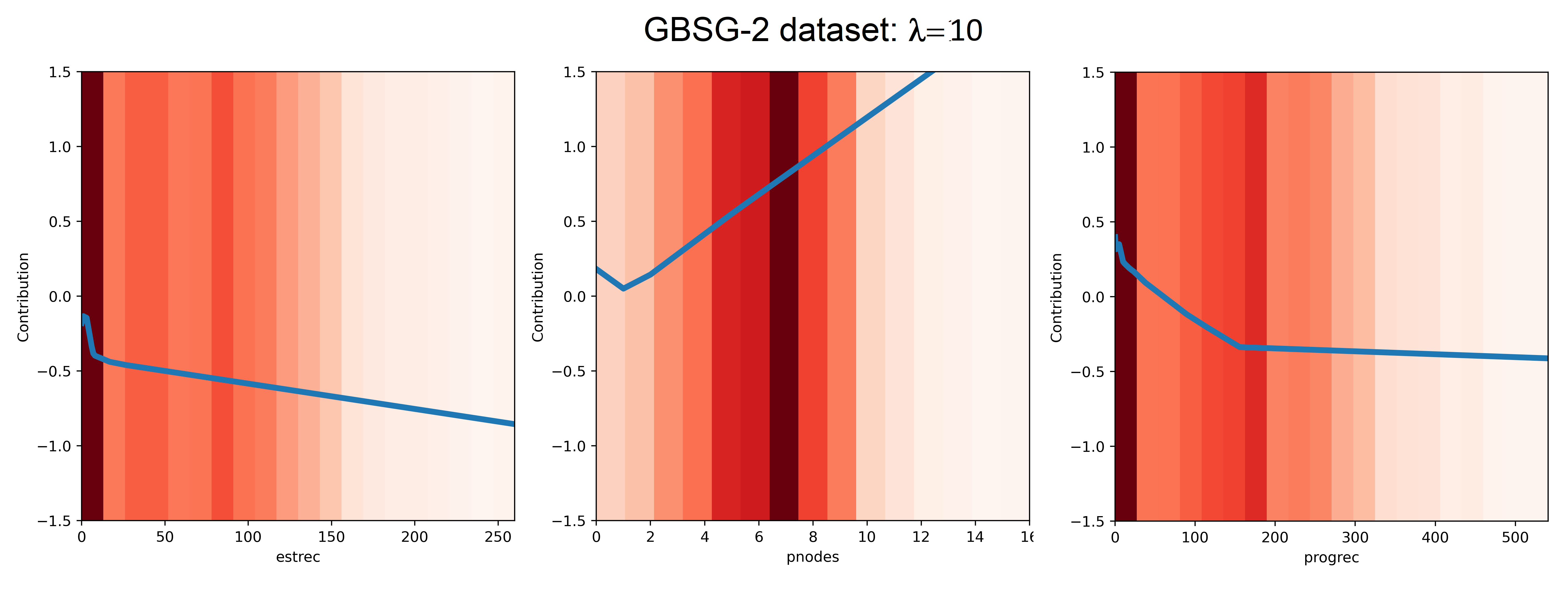
Figure 21: Shape functions for three important features obtained by means of the first modification of SurvNAM for the dataset GBSG2 and the local explanation by $\lambda=10$

Let us consider now the dataset MGUS2 which has illustrated a strange behavior of the shape function for the feature “creat” (creatinine) in Fig. 10. The shape function of the feature obtained by using the first modification of SurvNAM with the hyperparameter $\lambda=10000$ is depicted in Fig. 22. Smaller values of $\lambda$ do not impact on the form of the shape function. This implies that small values of parameters $\beta_{k}$ are compensated by large values of functions $g_{k}$. This undesirable property can be resolved by restricting values of functions $g_{k}$, by introducing the shortcut connection, and using the $L_{2}$ regularization for the neural networks weights, i.e., by applying the second modification of SurvNAM.

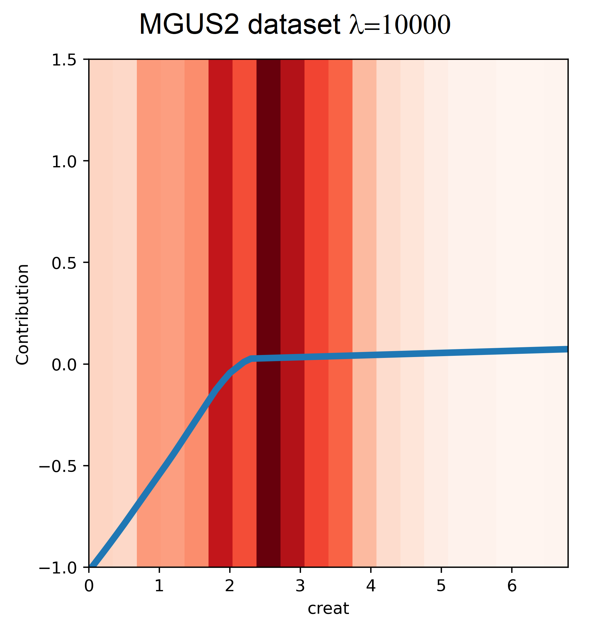
Figure 22: Shape functions for feature “creat” obtained by means of the first modification of SurvNAM for the dataset MGUS2 and the local explanation by $\lambda=10000$

The second modification of SurvNAM based on the shortcut connection is also studied by analyzing three important features “estrec”, “pnodes”, “progrec” of the dataset GBSG2, which show possible overfitting of the neural network. The network is trained by using the loss function (16) where hyperparameters $\lambda$ and $\mu$ are taken as $10$ and $1$, respectively. The corresponding shape functions are shown in Fig. 23. It can be seen from Fig. 23 that artifacts, which take place in Fig. 6 as well as in Fig. 21, are eliminated for all features. This implies that the network is not overfitted. It is interesting to see how values of $\alpha_{k}$ and $\omega_{k}$ allocated to features. Table 1 provides these values for numerical features. One can see from Table 1 that features “pnodes” and “tsize” do not use the non-linear part (functions $g_{k}$) and the corresponding shape functions are represented as linear functions whereas features “estrec” and “progrec” cannot be represented by the linear functions. It can clearly be seen for feature “progrec”. It is important to point out that restrictions on $\mathbf{W}$ in the form of the regularization term $\left\|\mathbf{W}\right\|_{2}^{2}$ do not allow functions $g_{k}$ to unboundedly increase.

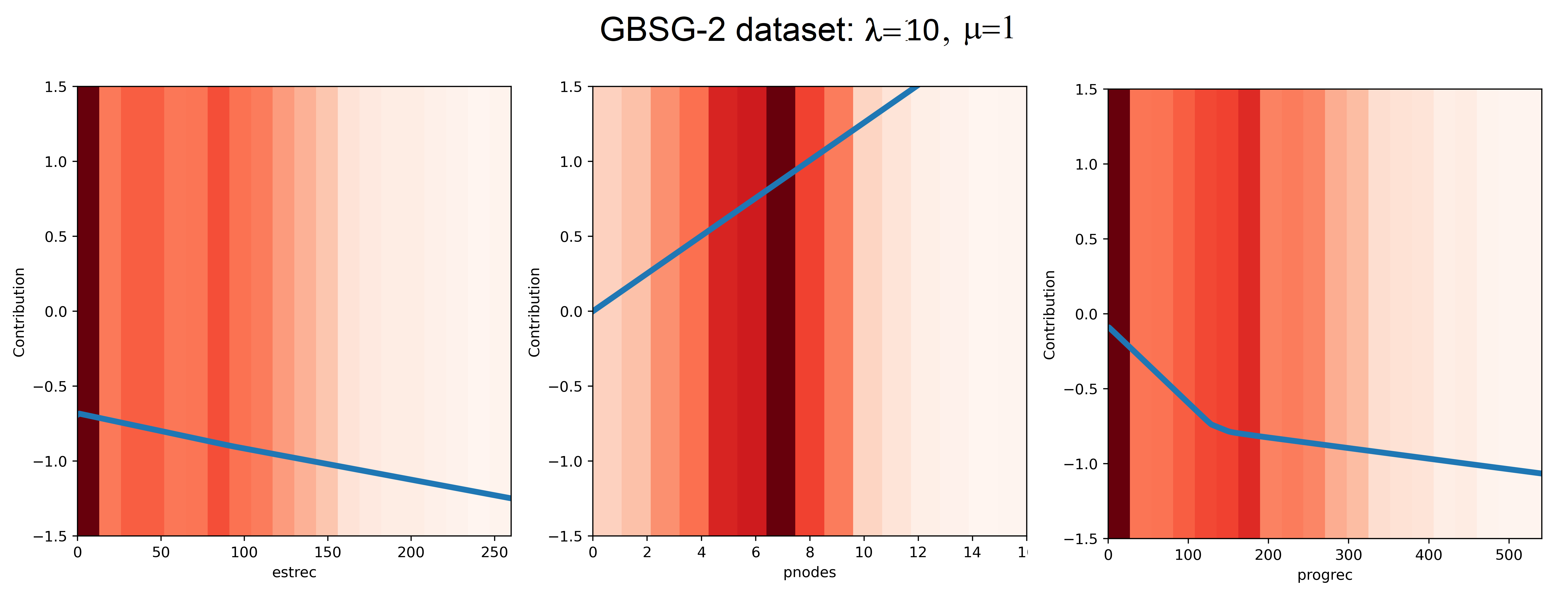
Figure 23: Shape functions for three important features obtained by means of the second modification of SurvNAM with the shortcut connection for the dataset GBSG2 and the local explanation by $\lambda=10$ and $\mu=1$

Table 1: Training parameters $\alpha_{k}$ and $\omega_{k}$ of the neural network trained on the dataset GBSG2 in accordance with the shortcut connection modification

Features	age	estrec	pnodes	progrec	tsize
$\alpha_{k}$	$0.315$	$0.775$	$0$	$0.929$	$0$
$1-\alpha_{k}$	$0.685$	$0.225$	$1.000$	$0.071$	$1$
$\omega_{k}$	$0.006$	$0.315$	$0.315$	$0.315$	$0.315$
$(1-\alpha_{k})\omega_{k}$	$0.004$	$0.071$	$0.315$	$0.022$	$0.315$

Similar results are obtained for the dataset MGUS2. Shape functions for the feature “creat” obtained by means of the second modification of SurvNAM with the shortcut connection by three values of $\lambda=0.01$, $0.1$, $1$ and $\mu=0.01$ are shown in Fig. 24. It can be seen from Fig. 24 how the linear part of the loss function begins to dominate with increase of the hyperparameter $\lambda$. The corresponding parameters $\alpha_{k}$, $\omega_{k}$ and their combinations by $\lambda=0.01$ and $\lambda=1$ are represented in Table 2. One can compare values of parameters for different strengths of the regularization. It is interesting to note that $\alpha_{k}$ for the “bad” feature “creat” changes from $0.922$ by $\lambda=0.01$ till $0$ by $\lambda=1$. This implies that linear part of the loss function totally dominates when $\lambda=1$. This fact is confirmed by the corresponding pictures in Fig. 24.

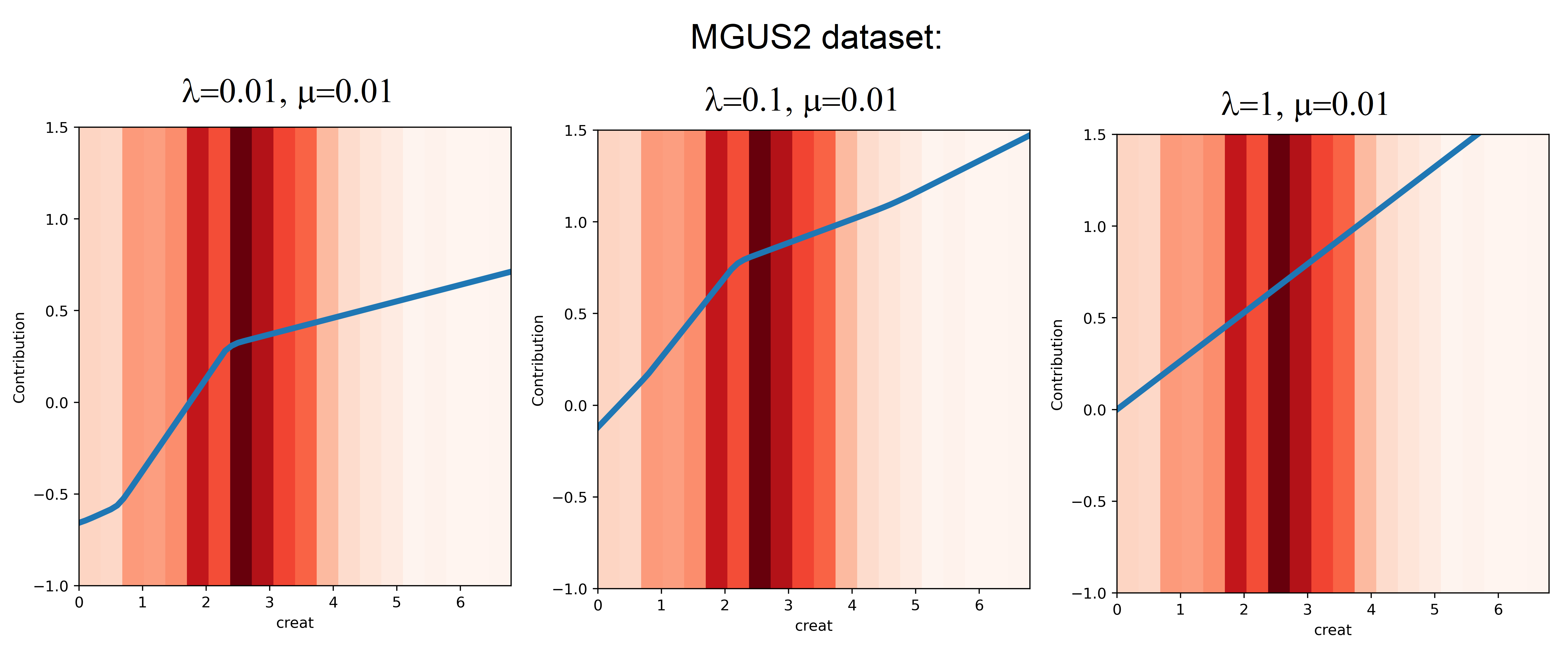
Figure 24: Shape functions for the feature “creat” obtained by means of the second modification of SurvNAM with the shortcut connection for the dataset MGUS2 and the local explanation by different values of $\lambda$ and $\mu=0.01$

Table 2: Training parameters $\alpha_{k}$ and $\omega_{k}$ of the neural network trained on the dataset MGUS2 in accordance with the shortcut connection modification

	$\lambda=0.01$				$\lambda=1$
Features	age	hgb	creat	mspike	age	hgb	creat	mspike
$\alpha_{k}$	$0.976$	$0.995$	$0.922$	$0.820$	$0.788$	$0.262$	$0$	$0$
$1-\alpha_{k}$	$0.024$	$0.005$	$0.078$	$0.180$	$0.212$	$0.738$	$1$	$1$
$\omega_{k}$	$0.830$	$0.765$	$1.095$	$1.012$	$0.861$	$0.768$	$0.264$	$0.489$
$(1-\alpha_{k})\omega_{k}$	$0.020$	$0.004$	$0.085$	$0.182$	$0.183$	$0.567$	$0.264$	$0.489$

8 SurvNAM vs. SurvLIME

An explanation method called SurvLIME has been proposed by Kovalev et al. [21]. This method also explains predictions of the black-box survival models. Therefore, one of the important questions is how SurvNAM and SurvLIME relate with each other.

First, they solve the same task of the survival model explanation. However, SurvLIME solves only a task of the local explanation whereas SurvNAM can solve the local as well as global explanations. As a result, SurvLIME uses only perturbation technique whereas SurvNAM may use only the training set if the global explanation is aimed.

Second, both the methods are based on the Cox model approximation. This is the basic idea behind the methods. However, SurvLIME is based on using the original Cox model with linear relationship between covariates whereas SurvNAM uses an extension of the Cox model for approximation. According to the extension, the sum of some functions of covariates is used instead of their simple linear sum. As a result, the extended Cox model may significantly improve its approximation to the explained model.

Third, SurvLIME solves a complex optimization problem for computing coefficients of covariates in the Cox model whereas the neural network is trained in SurvNAM. In fact, the neural network also implicitly solves the convex optimization problem. However, it is more flexible from the point of view of various optimization variants. In particular, various types of the regularization can be added to SurvNAM whereas SurvLIME is restricted only by regularizations which remain the optimization problem in the classes of linear and quadratic programming problems.

Fourth, SurvLIME provides the explanation results in the form of coefficients reflecting the feature impacts on predictions whereas SurvNAM provides the feature contribution functions which indirectly show the feature impact. One can see from the shape functions how the contribution of each feature changes with change of its values.

It can be seen from the above that SurvNAM and SurvLIME have many common elements, but these elements have the different content. It is difficult to evaluate which method is better. Every method has advantages and disadvantages. For example, on the one hand, SurvLIME solves the quadratic optimization problem which has a unique solution and can be exactly solves by several available algorithms. SurvNAM requires training the neural network which can be overfitted or just can provide inaccurate predictions. On the other hand, the neural network is a more flexible tool and can provide direction for various extensions and modifications of SurvNAM. On the one hand, the neural network can deal with very complex objects, for example, with images. Therefore, SurvNAM has the important advantage in comparison with SurvLIME. On the other hand, it is difficult to construct and to train the neural network when the number of features is very large in SurvNAM whereas SurvLIME can deal with the large number of features because the number of features weakly impact on the optimization problem complexity. Though we have to point out that the number of features impact on the perturbation procedure.

We see again that both the methods are comparable. Nevertheless, SurvNAM is more flexible, its results are more informative, it has great potentialities for extending and for solving more complex survival problems than SurvLIME.

9 Conclusion

Among various distances between the predictions of the black-box model and the extended Cox model applied to constructing the loss function, we have considered only the Euclidean distance. However, it is also interesting to study other metrics which preserve the loss function convexity, for example, the Manhattan distance (the $L_{1}$-norm) and the Chebyshev distance (the $L_{\infty}$-norm). These distances may provide unexpected results whose studying is a direction for further research.

There are two main difficulties of the proposed method. First, it represents results in the form of the feature shape functions as measures of the feature importance. However, explanations are simpler if they are represented by a single number measuring the feature importance. Second, the method uses neural networks which may be overfitted and require many examples for their training. One of the approaches overcoming the above difficulties is the ensemble of gradient boosting machines [76]. An extension of this approach to the survival model explanation problem may be an interesting direction for further research.

Another interesting problem is to consider how combinations of correlated features impact on the survival model prediction. A direct way is to train $2^{m}$ neural subnetworks such that each pair of features is fed to each subnetwork. This way requires to train $2^{m}$ subnetworks. Therefore, another approach should be developed to take into account correlated features. This is a direction for further research.

It is interesting to investigate how different regularization terms impact on results. We have illustrated how the well-known Lasso method with the corresponding regularization term can be applied to removing unimportant shape functions in the extended Cox model and improves the results. However, other regularization methods can be of the large interest. It should be also noted that the shortcut connection trick used in the proposed modifications of SurvNAM can be also applied to other tasks different from the survival model explanation. We have not also studied how time-dependent features might change the proposed approach. The above questions can be viewed as directions for further research.

The proposed method is efficient mainly for tabular data. However, it can be also adapted to the image processing which has some inherent peculiarities. The adaptation is another interesting direction for research in future.

References

- [1] A. Holzinger, G. Langs, H. Denk, K. Zatloukal, and H. Muller. Causability and explainability of artificial intelligence in medicine. WIREs Data Mining and Knowledge Discovery, 9(4):e1312, 2019.
- [2] V. Arya, R.K.E. Bellamy, P.-Y. Chen, A. Dhurandhar, M. Hind, S.C. Hoffman, S. Houde, Q.V. Liao, R. Luss, A. Mojsilovic, S. Mourad, P. Pedemonte, R. Raghavendra, J. Richards, P. Sattigeri, K. Shanmugam, M. Singh, K.R. Varshney, D. Wei, and Y. Zhang. One explanation does not fit all: A toolkit and taxonomy of AI explainability techniques. arXiv:1909.03012, Sep 2019.
- [3] V. Belle and I. Papantonis. Principles and practice of explainable machine learning. arXiv:2009.11698, September 2020.
- [4] R. Guidotti, A. Monreale, S. Ruggieri, F. Turini, F. Giannotti, and D. Pedreschi. A survey of methods for explaining black box models. ACM computing surveys, 51(5):93, 2019.
- [5] Y. Liang, S. Li, C. Yan, M. Li, and C. Jiang. Explaining the black-box model: A survey of local interpretation methods for deep neural networks. Neurocomputing, 419:168–182, 2021.
- [6] C. Molnar. Interpretable Machine Learning: A Guide for Making Black Box Models Explainable. Published online, https://christophm.github.io/interpretable-ml-book/, 2019.
- [7] W.J. Murdoch, C. Singh, K. Kumbier, R. Abbasi-Asl, and B. Yua. Interpretable machine learning: definitions, methods, and applications. arXiv:1901.04592, Jan 2019.
- [8] N. Xie, G. Ras, M. van Gerven, and D. Doran. Explainable deep learning: A field guide for the uninitiated. arXiv:2004.14545, April 2020.
- [9] E. Zablocki, H. Ben-Younes, P. Perez, and M. Cord. Explainability of vision-based autonomous driving systems: Review and challenges. arXiv:2101.05307, January 2021.
- [10] Y. Zhang, P. Tino, A. Leonardis, and K. Tang. A survey on neural network interpretability. arXiv:2012.14261, December 2020.
- [11] M.T. Ribeiro, S. Singh, and C. Guestrin. “Why should I trust You?” Explaining the predictions of any classifier. arXiv:1602.04938v3, Aug 2016.
- [12] T. Hastie and R. Tibshirani. Generalized additive models, volume 43. CRC press, 1990.
- [13] H. Nori, S. Jenkins, P. Koch, and R. Caruana. InterpretML: A unified framework for machine learning interpretability. arXiv:1909.09223, September 2019.
- [14] R. Agarwal, N. Frosst, X. Zhang, R. Caruana, and G.E. Hinton. Neural additive models: Interpretable machine learning with neural nets. arXiv:2004.13912, April 2020.
- [15] Z. Yang, A. Zhang, and A. Sudjianto. Gami-net: An explainable neural networkbased on generalized additive models with structured interactions. arXiv:2003.07132, March 2020.
- [16] J. Chen, J. Vaughan, V.N. Nair, and A. Sudjianto. Adaptive explainable neural networks (AxNNs). arXiv:2004.02353v2, April 2020.
- [17] D. Hosmer, S. Lemeshow, and S. May. Applied Survival Analysis: Regression Modeling of Time to Event Data. John Wiley & Sons, New Jersey, 2008.
- [18] P. Wang, Y. Li, and C.K. Reddy. Machine learning for survival analysis: A survey. ACM Computing Surveys (CSUR), 51(6):1–36, 2019.
- [19] D.R. Cox. Regression models and life-tables. Journal of the Royal Statistical Society, Series B (Methodological), 34(2):187–220, 1972.
- [20] M.S. Kovalev and L.V. Utkin. A robust algorithm for explaining unreliable machine learning survival models using the Kolmogorov-Smirnov bounds. Neural Networks, 132:1–18, 2020.
- [21] M.S. Kovalev, L.V. Utkin, and E.M. Kasimov. SurvLIME: A method for explaining machine learning survival models. Knowledge-Based Systems, 203:106164, 2020.
- [22] L.V. Utkin, M.S. Kovalev, and E.M. Kasimov. An explanation method for black-box machine learning survival models using the chebyshev distance. In Artificial Intelligence and Natural Language. AINL 2020, volume 1292 of Communications in Computer and Information Science, pages 62–74, Cham, 2020. Springer.
- [23] S.M. Shankaranarayana and D. Runje. ALIME: Autoencoder based approach for local interpretability. arXiv:1909.02437, Sep 2019.
- [24] I. Ahern, A. Noack, L. Guzman-Nateras, D. Dou, B. Li, and J. Huan. NormLime: A new feature importance metric for explaining deep neural networks. arXiv:1909.04200, Sep 2019.
- [25] M.R. Zafar and N.M. Khan. DLIME: A deterministic local interpretable model-agnostic explanations approach for computer-aided diagnosis systems. arXiv:1906.10263, Jun 2019.
- [26] M.T. Ribeiro, S. Singh, and C. Guestrin. Anchors: High-precision model-agnostic explanations. In AAAI Conference on Artificial Intelligence, pages 1527–1535, 2018.
- [27] L. Hu, J. Chen, V.N. Nair, and A. Sudjianto. Locally interpretable models and effects based on supervised partitioning (LIME-SUP). arXiv:1806.00663, Jun 2018.
- [28] J. Rabold, H. Deininger, M. Siebers, and U. Schmid. Enriching visual with verbal explanations for relational concepts: Combining LIME with Aleph. arXiv:1910.01837v1, October 2019.
- [29] Q. Huang, M. Yamada, Y. Tian, D. Singh, D. Yin, and Y. Chang. GraphLIME: Local interpretable model explanations for graph neural networks. arXiv:2001.06216, January 2020.
- [30] E. Strumbelj and I. Kononenko. An efficient explanation of individual classifications using game theory. Journal of Machine Learning Research, 11:1–18, 2010.
- [31] S.M. Lundberg and S.-I. Lee. A unified approach to interpreting model predictions. In Advances in Neural Information Processing Systems, pages 4765–4774, 2017.
- [32] P.W. Koh and P. Liang. Understanding black-box predictions via influence functions. In Proceedings of the 34th International Conference on Machine Learning, volume 70, pages 1885–1894, 2017.
- [33] C. Burns, J. Thomason, and W. Tansey. Interpreting black box models with statistical guarantees. arXiv:1904.00045, Mar 2019.
- [34] S. Wachter, B. Mittelstadt, and C. Russell. Counterfactual explanations without opening the black box: Automated decisions and the GPDR. Harvard Journal of Law & Technology, 31:841–887, 2017.
- [35] Y. Goyal, Z. Wu, J. Ernst, D. Batra, D. Parikh, and S. Lee. Counterfactual visual explanations. arXiv:1904.07451, Apr 2019.
- [36] L.A. Hendricks, R. Hu, T. Darrell, and Z. Akata. Grounding visual explanations. In Proceedings of the European Conference on Computer Vision (ECCV), pages 264–279, 2018.
- [37] A. Van Looveren and J. Klaise. Interpretable counterfactual explanations guided by prototypes. arXiv:1907.02584, Jul 2019.
- [38] J. van der Waa, M. Robeer, J. van Diggelen, M. Brinkhuis, and M. Neerincx. Contrastive explanations with local foil trees. arXiv:1806.07470, June 2018.
- [39] Y. Ramon, D. Martens, F. Provost, and T. Evgeniou. Counterfactual explanation algorithms for behavioral and textual data. arXiv:1912.01819, December 2019.
- [40] A. White and A.dA. Garcez. Measurable counterfactual local explanations for any classifier. arXiv:1908.03020v2, November 2019.
- [41] R. Fong and A. Vedaldi. Explanations for attributing deep neural network predictions. In Explainable AI, volume 11700 of LNCS, pages 149–167. Springer, Cham, 2019.
- [42] R.C. Fong and A. Vedaldi. Interpretable explanations of black boxes by meaningful perturbation. In Proceedings of the IEEE International Conference on Computer Vision, pages 3429–3437. IEEE, 2017.
- [43] V. Petsiuk, A. Das, and K. Saenko. RISE: Randomized input sampling for explanation of black-box models. arXiv:1806.07421, June 2018.
- [44] M.N. Vu, T.D. Nguyen, N. Phan, and M.T. Thai R. Gera. Evaluating explainers via perturbation. arXiv:1906.02032v1, Jun 2019.
- [45] M. Du, N. Liu, and X. Hu. Techniques for interpretable machine learning. arXiv:1808.00033, May 2019.
- [46] A. Adadi and M. Berrada. Peeking inside the black-box: A survey on explainable artificial intelligence (XAI). IEEE Access, 6:52138–52160, 2018.
- [47] A.B. Arrieta, N. Diaz-Rodriguez, J. Del Ser, A. Bennetot, S. Tabik, A. Barbado, S. Garcia, S. Gil-Lopez, D. Molina, R. Benjamins, R. Chatila, and F. Herrera. Explainable artificial intelligence (XAI): Concepts, taxonomies, opportunities and challenges toward responsible AI. arXiv:1910.10045, October 2019.
- [48] D.V. Carvalho, E.M. Pereira, and J.S. Cardoso. Machine learning interpretability: A survey on methods and metrics. Electronics, 8(832):1–34, 2019.
- [49] C. Rudin. Stop explaining black box machine learning models for high stakes decisions and use interpretable models instead. Nature Machine Intelligence, 1:206–215, 2019.
- [50] C. Rudin, C. Chen, Z. Chen, H. Huang, L. Semenova, and C. Zhong. Interpretable machine learning: Fundamental principles and 10 grand challenges. arXiv:2103.11251, March 2021.
- [51] R. Tibshirani. The lasso method for variable selection in the cox model. Statistics in medicine, 16(4):385–395, 1997.
- [52] S. Kaneko, A. Hirakawa, and C. Hamada. Enhancing the lasso approach for developing a survival prediction model based on gene expression data. Computational and Mathematical Methods in Medicine, 2015(Article ID 259474):1–7, 2015.
- [53] J. Kim, I. Sohn, S.-H. Jung, S. Kim, and C. Park. Analysis of survival data with group lasso. Communications in Statistics - Simulation and Computation, 41(9):1593–1605, 2012.
- [54] N. Ternes, F. Rotolo, and S. Michiels. Empirical extensions of the lasso penalty to reduce the false discovery rate in high-dimensional cox regression models. Statistics in medicine, 35(15):2561–2573, 2016.
- [55] D.M. Witten and R. Tibshirani. Survival analysis with high-dimensional covariates. Statistical Methods in Medical Research, 19(1):29–51, 2010.
- [56] H.H. Zhang and W. Lu. Adaptive Lasso for Cox’s proportional hazards model. Biometrika, 94(3):691–703, 2007.
- [57] V. Van Belle, K. Pelckmans, S. Van Huffel, and J.A. Suykens. Support vector methods for survival analysis: a comparison between ranking and regression approaches. Artificial intelligence in medicine, 53(2):107–118, 2011.
- [58] D. Faraggi and R. Simon. A neural network model for survival data. Statistics in medicine, 14(1):73–82, 1995.
- [59] C. Haarburger, P. Weitz, O. Rippel, and D. Merhof. Image-based survival analysis for lung cancer patients using CNNs. arXiv:1808.09679v1, Aug 2018.
- [60] J.L. Katzman, U. Shaham, A. Cloninger, J. Bates, T. Jiang, and Y. Kluger. Deepsurv: Personalized treatment recommender system using a Cox proportional hazards deep neural network. BMC medical research methodology, 18(24):1–12, 2018.
- [61] R. Ranganath, A. Perotte, N. Elhadad, and D. Blei. Deep survival analysis. arXiv:1608.02158, September 2016.
- [62] X. Zhu, J. Yao, and J. Huang. Deep convolutional neural network for survival analysis with pathological images. In 2016 IEEE International Conference on Bioinformatics and Biomedicine, pages 544–547. IEEE, 2016.
- [63] N.A. Ibrahim, A. Kudus, I. Daud, and M.R. Abu Bakar. Decision tree for competing risks survival probability in breast cancer study. International Journal Of Biological and Medical Research, 3(1):25–29, 2008.
- [64] U.B. Mogensen, H. Ishwaran, and T.A. Gerds. Evaluating random forests for survival analysis using prediction error curves. Journal of Statistical Software, 50(11):1–23, 2012.
- [65] J.B. Nasejje, H. Mwambi, K. Dheda, and M. Lesosky. A comparison of the conditional inference survival forest model to random survival forests based on a simulation study as well as on two applications with time-to-event data. BMC Medical Research Methodology, 17(115):1–17, 2017.
- [66] I.K. Omurlu, M. Ture, and F. Tokatli. The comparisons of random survival forests and cox regression analysis with simulation and an application related to breast cancer. Expert Systems with Applications, 36:8582–8588, 2009.
- [67] M. Schmid, M.N. Wright, and A. Ziegler. On the use of harrell’s c for clinical risk prediction via random survival forests. Expert Systems with Applications, 63:450–459, 2016.
- [68] H. Wang and L. Zhou. Random survival forest with space extensions for censored data. Artificial intelligence in medicine, 79:52–61, 2017.
- [69] M.N. Wright, T. Dankowski, and A. Ziegler. Random forests for survival analysis using maximally selected rank statistics. arXiv:1605.03391v1, May 2016.
- [70] M.N. Wright, T. Dankowski, and A. Ziegler. Unbiased split variable selection for random survival forests using maximally selected rank statistics. Statistics in Medicine, 36(8):1272–1284, 2017.
- [71] J.H. Friedman. Greedy function approximation: A gradient boosting machine. Annals of Statistics, 29:1189–1232, 2001.
- [72] J.H. Friedman. Stochastic gradient boosting. Computational statistics & data analysis, 38(4):367–378, 2002.
- [73] Y. Lou, R. Caruana, and J. Gehrke. Intelligible models for classification and regression. In Proceedings of the 18th ACM SIGKDD International Conference on Knowledge Discovery and Data Mining, pages 150–158. ACM, August 2012.
- [74] X. Zhang, S. Tan, P. Koch, Y. Lou, U. Chajewska, and R. Caruana. Axiomatic interpretability for multiclass additive models. In In Proceedings of the 25th ACM SIGKDD International Conference on Knowledge Discovery & Data Mining, pages 226–234. ACM, 2019.
- [75] C.-H. Chang, S. Tan, B. Lengerich, A. Goldenberg, and R. Caruana. How interpretable and trustworthy are gams? arXiv:2006.06466, June 2020.
- [76] A.V. Konstantinov and L.V. Utkin. Interpretable machine learning with an ensemble of gradient boosting machines. Knowledge-Based Systems, 222(106993):1–16, 2021.
- [77] F. Harrell, R. Califf, D. Pryor, K. Lee, and R. Rosati. Evaluating the yield of medical tests. Journal of the American Medical Association, 247:2543–2546, 1982.
- [78] K. Devarajn and N. Ebrahimi. A semi-parametric generalization of the cox proportional hazards regression model: Inference and applications. Computational Statistics & Data Analysis, 55(1):667–676, 2011.
- [79] M.Z. Nezhad, N. Sadati, K. Yang, and D. Zhu. A deep active survival analysis approach for precision treatment recommendations: Application of prostate cancer. arXiv:1804.03280v1, April 2018.
- [80] S. Polsterl, N. Navab, and A. Katouzian. An efficient training algorithm for kernel survival support vector machines. arXiv:1611.07054v, Nov 2016.
- [81] A. Bender, A. Groll, and F. Scheipl. A generalized additive model approach to time-to-event analysis. Statistical Modelling, 18(3-4):1–23, 2018.
- [82] T. Hastie and R. Tibshirani. Generalized additive models for medical research. Statistical Methods in Medical Research, 4:187–196, 1995.
- [83] P. Ravikumar, H. Liu, J. Lafferty, and L. Wasserman. Sparse additive models. Journal of the Royal Statistical Society: Series B (Statistical Methodology), 71(5):1009–1030, 2009.
- [84] M. Avalos, Y. Grandvalet, and C. Ambroise. Regularization methods for additive models. In Advances in Intelligent Data Analysis V. IDA 2003, volume 2810 of Lecture Notes in Computer Science, pages 509–520, Berlin, Heidelberg, 2003. Springer.
- [85] A. Haris, N. Simon, and A. Shojaie. Generalized sparse additive models. arXiv:1903.04641, Mar 2019.
- [86] K. He, X. Zhang, S. Ren, and J. Sun. Deep residual learning for image recognition. In Proceedings of the IEEE conference on computer vision and pattern recognition, pages 770–778, 2016.
- [87] T. Liu, M. Chen, M. Zhou, S. Du, E. Zhou, and T. Zhao. Towards understanding the importance of shortcut connections in residual networks. arXiv:1909.04653, Sep 2019.
- [88] L. Breiman. Random forests. Machine learning, 45(1):5–32, 2001.