Dissipative phase transition in a spatially-correlated bosonic bath

Abstract

The presence of symmetries in a closed many-body quantum system results in integrability. For such integrable systems, complete thermalization does not occur. As a result, the system remains non-ergodic. On the other hand, a set of non-interacting atoms connected to a regular bosonic bath thermalizes. Here, we show that such atoms in a spatially-correlated thermal bath can show both the behavior depending on the temperature. At zero temperature, the bath has a large correlation length, and hence it acts as a common environment. In this condition, a set of weak symmetries exist, which prevent thermalization. The system undergoes a symmetry-broken dissipative phase transition of the first order as the temperature rises above zero.

I Introduction

The irreversible journey of closed or open quantum systems towards thermal equilibrium, i.e., the thermalization problem, has been the subject of intense research for many decades. For a set of classical particles, Boltzmann suggested an explanation based on the collisions Kardar (2007). Later, in 1929, von Neumann proposed the quantum ergodic theorem, which is the first step towards the quantum thermalization problem von Neumann (2010). About three decades ago, Srednicki proposed the famous eigenstate-thermalization hypothesis (ETH) for a closed many-particle system. According to ETH, a specific state of a closed interacting many-particle quantum system would thermalize, provided that state’s energy eigenstate representation obeys Berry’s conjecture Srednicki (1994). For such a system, the ensemble average of an observable reaches the thermal expectation value after a long time. One can partition such a system into a chosen subsystem, and an effective heat bath from the remainder of the system Nandkishore and Huse (2015). Consequently, the von Neumann entropy of the subsystems is extensive, and it follows the volume law Abanin et al. (2019).

Closed many-body systems may not thermalize if they are in a localized state. Anderson showed the non-thermal nature of the disordered systems, known as Anderson localization Anderson (1958). There exist several integrals of motion from the symmetry of the system, which break the principle of equal apriori probabilities. Therefore, integrability remains one of the measures of the non-thermal phases. Many-body localization (MBL), quantum scars are the examples where the ETH fails due to the presence of symmetries Abanin et al. (2019); Pal and Huse (2010); Oganesyan and Huse (2007); Turner et al. (2018). MBL eigenstates are known to follow the area-law entanglement in place of the volume law. The subsystems become entangled in the localized phase Abanin et al. (2019).

On the other hand, the system is coupled to a thermal bath with a specific temperature for the open quantum system. The system-bath interaction remains the source of thermalization, and the quantum master equation describes the reduced dynamics of the system Heinz-Peter Breuer (2002); Kossakowski (1972). The system inherits the temperature from the bath. For example, the Bloch equation for spin-$1/2$ particles successfully describes the dynamical evolution toward equilibrium configuration Bloch (1946).

In dissipative quantum systems, transitions can happen between thermal to non-thermal phases. The steady-state solution of the master equation is, in general, a function of the parameters of the system and the bath. At a critical value of the parameters, the steady-state configuration may undergo a sudden change. The more detailed analysis involves the study of the eigenvalues of the Lindbladian. The thermal steady-state corresponds to the zero eigenvalue of the Lindbladian. The eigenvalue with the smallest non-zero absolute value provides the asymptotic decay rate (ADR), which determines the rate of approach to the steady-state. If a continuous change of a system parameter results in the vanishing of the ADR and an emergence of a dark state, then such a change is termed a dissipative phase transition (DPT) Kessler et al. (2012); Albert and Jiang (2014); Horstmann et al. (2013); Buča and Prosen (2012); Manzano and Hurtado (2014); Minganti et al. (2018); Lieu et al. (2020). The vanishing of ADR ensures that the dark state does not evolve under system-bath coupling Hamiltonian Buča and Prosen (2012). As such, such states are often described as a decoherence-free sub-space in quantum optics and quantum computation Fleischhauer and Lukin (2002); Mohapatra et al. (2008). DPT is closely related to the symmetry-breaking transitions Albert and Jiang (2014); Lieu et al. (2020); Manzano and Hurtado (2014). A thermal phase is a symmetry-broken phase due to its lack of integrability. For such systems, the final steady-state is unique, and all the memory of initial states are lost Nandkishore and Huse (2015). On the other hand, the non-thermal phases are protected by several symmetry operators. Hence the final steady-state in that case has the initial value dependence, and there exist different integrals of motions along with the total energy Kessler et al. (2012).

In this work, we show that a spatially-correlated bosonic bath can connect the two extreme cases described above. We consider a set of non-interacting quantum systems weakly coupled to a spatially-correlated bosonic bath. The bath correlation function generally decays over finite length for a spatially-correlated bath Jeske and Cole (2013a); McCutcheon et al. (2009). At zero temperature, the bath acts as a common environment. Hence, a cooperative effect between a pair of systems is observed in the form of an entanglement Braun (2002); Benatti et al. (2003); Carmichael (1980). The bath-induced entanglement helps the system to escape the thermal steady state. We also identify the weak symmetry operators, which are preserved during the dynamics. As the temperature increases, the bath’s correlation length becomes shorter, and the spin-pairs are disentangled. As the entanglement vanishes, the system reaches a thermal Gibb’s state. We find out the weak symmetry broken phase transition at the critical point of the temperature. We find that the phase transition is similar to the thermal-to-localized phase transition observed in closed many-body systems. There is the possibility of getting a non-thermal phase at non-zero temperature if we make the bath correlation length much longer. Reservoir engineering, which involves adjusting the parameters of a bath, is an efficient technique for creating such a non-thermal atomic state in optical cavities and ion trap experiments Poyatos et al. (1996a); Plenio and Huelga (2002); Bose et al. (1999). With the increase in the number of atoms, the number of integrable quantities increases, and the von Neumann entropy is no longer extensive.

II Non-interacting systems in a spatially-correlated bath

We consider two non-interacting spins coupled to a bosonic bath. We shall generalize the result to multiple systems later in the manuscript. The total Hamiltonian for these systems and the bath is given by,

$$\mathcal{H}=\sum\limits_{m=1}^{2}\mathcal{H}_{ms}^{0}+\mathcal{H}_{L}^{0}+\mathcal{H}_{\text{\tiny SL}}$$ (1)

where, $\mathcal{H}_{1s}^{0},\mathcal{H}_{2s}^{0}$ are the Zeeman Hamiltonians of the spins. $\mathcal{H}_{(1,2)s}=\omega^{(1,2)}_{0}\sigma_{3}^{(1,2)}/2$, where, $\omega_{\circ}$ is the Larmor frequency and $\sigma_{i}$s are the Pauli spin matrices. $\mathcal{H}_{L}^{0}$ is the free Hamiltonian of the bosonic bath, given by $\mathcal{H}_{L}^{0}=\sum\limits_{k}\omega_{k}a^{\dagger}_{k}a_{k}$. The spins are weakly-coupled to the bath. We use the coupling Hamiltonian $\mathcal{H}_{\text{\tiny SL}}$ adapted from a spatially-correlated spin-boson model McCutcheon et al. (2009). As such, we have $\mathcal{H}_{\text{\tiny SL}}=\sum\limits_{m=1}^{2}(\sigma^{m}_{+}\mathcal{L}_{m}+\sigma^{m}_{-}\mathcal{L}^{\dagger}_{m})$, where $\mathcal{L}_{m}$ is the corresponding bath modes. The bath modes are defined as, $\mathcal{L}_{m}(r)=\sum\limits_{k}g_{k}^{m}a_{k}$. Here, $g_{k}^{m}$ is the coupling amplitude of the $m$th spin and the bosonic bath and is given by $g_{k}^{m}=g_{k}e^{ikr_{m}}$. Hence, $g_{k}^{1}\neq g_{k}^{2}$ but $|g_{k}^{1}|=|g_{k}^{2}|$. Two spins has a spatial separation, $d=|r_{1}-r_{2}|$. In the interaction representation of the free Hamiltonian, the dynamical equations of the reduced density matrix of the spins is given by the coarse-grained quantum master equation (QME) Heinz-Peter Breuer (2002). The bath is assumed to be in thermal equilibrium, so the equilibrium density matrices are given by, $\rho_{L}^{eq}=e^{-\beta\mathcal{H}_{L}^{0}}/\mathcal{Z}_{L}$, where, $\mathcal{Z}_{L}$ is the partition function of the bath, and $\beta$ is the inverse temperature of the bath, so $T=1/\beta$. The initial correlation between the system and bath are neglected (Born-Markov approximation) Claude Cohen-Tannoudji (1998). Also, it follows from the definition of $\mathcal{H}_{\text{\tiny SL}}$ that ${\rm Tr}_{\text{\tiny L}}\{\mathcal{H}_{\text{\tiny SL}}\rho_{L}^{eq}\}=0$, which ensures that the system-local environment coupling only contributes in the second-order.

After Jeske and others, we consider a one-dimensional chain of spatially located, coupled harmonic oscillators, the “tight-binding chain” as was originally named by by the authors and the spatial correlations decay over a characteristic correlation length $\xi=2\omega\beta g_{b}$, resulting from the excitations hopping along the chain and thermal noise. Here, $\omega$ is the bath lattice spacing, $g_{b}$ is the coupling between the neighboring bath oscillators, and $\beta$ is the inverse temperature Jeske and Cole (2013b). We assume both the temporal and spatial bath correlations are stationary in time and space Jeske and Cole (2013b). Bath spectral density functions corresponding to $\sigma^{n}_{-}\sigma^{m}_{+}$ and $\sigma^{n}_{+}\sigma^{m}_{-}$ terms (The second-order terms of $\mathcal{H}_{\text{\tiny SL}}$ ), for $n\neq m,\{n,m\}\in\{1,2\},$ in the dissipator are, respectively, given as,

$$\Gamma_{mn}(\omega_{\circ},r) = \sum\limits_{k}g_{k}^{m}{g_{k}^{n}}^{\star}\int\limits_{0}^{\infty}dte^{-i(\omega_{\circ}-\omega_{k})t}\langle a^{\dagger}_{k}a_{k}\rangle e^{-ik.r}$$

$$\Delta_{mn}(\omega_{\circ},r) = \sum\limits_{k}g_{k}^{n}{g_{k}^{m}}^{\star}\int\limits_{0}^{\infty}dte^{i(\omega_{\circ}-\omega_{k})t}\langle a_{k}a^{\dagger}_{k}\rangle e^{-ik.r}$$ (2)

In deriving the above, one encounters a double sum over $k$ and $k^{\prime}$ in the spectral density functions and $k\neq k^{\prime}$ cases vanish owing to differences in $\omega_{k}\neq\omega_{k^{\prime}}$ a situation akin to rotating wave approximation. For a bosonic bath, we have $\langle a_{k}a^{\dagger}_{k}\rangle=(1+N(\omega_{k}))$ and $\langle a^{\dagger}_{k}a_{k}\rangle=N(\omega_{k})$, where, $N(\omega_{k})=1/(\exp(\beta\omega_{k})-1)$.

To simplify the representation of the dynamical equation in the following, we also define $A_{mn}(\omega_{\circ},r)=\Gamma_{mn}(\omega_{\circ},r)+\Gamma_{mn}^{*}(\omega_{\circ},r)$, $B_{mn}(\omega_{\circ},r)=\Delta_{mn}(\omega_{\circ},r)+\Delta_{mn}^{*}(\omega_{\circ},r)$ and $J_{mn}(r)=\frac{1}{2i}(\Gamma_{mn}(\omega_{\circ},r)-\Gamma_{mn}^{*}(\omega_{\circ},r))$, $K_{mn}(r)=\frac{1}{2i}(\Delta_{mn}(\omega_{\circ},r)-\Delta_{mn}^{*}(\omega_{\circ},r))$.

For $n=m$, one obtains terms similar as the above, except the spectral densities do not have the $r-$dependent $e^{-ik.r}$ terms. In this limit, the bath spectral density functions contain a sum of Dirac deltas, $\sum\limits_{k}|g_{k}|^{2}\delta(\omega_{\circ}-\omega_{k})$. The spectral density terms, in this case, characterize a local environment and not a common environment.

We expect that the cross-terms from the common environment should vanish when the two qubits are far apart ($r\ll\xi$), i.e., when the temperature is high ($\beta\to 0$) corresponding to short spatial correlation length. On the other hand, when the two qubits are close ($r\gg\xi$), or the temperature goes to zero ($\beta\to\infty$), the common environment effect is the highest McCutcheon et al. (2009). In line with the previous works, it had been assumed that a $r$-dependent function (say, $\alpha(r)$ with $r=|\vec{r}_{1}-\vec{r}_{2}|$) could be chosen to scale the spectral density functions. This function must satisfy $\alpha(\infty)=0$, which ensures that the cross-terms from the common environment vanish when the two qubits are very far apart and $\beta\to\infty$ , and $\alpha(0)=1$, which ensures the maximum extent of the common environment effect. In earlier work, Jeske and others have proven that any dissipator with exponential or Gaussian spatial correlation function could be mapped to Lindblad form, ensuring CPTP. This allows the choice of an exponential form of $\alpha(r)=\exp(-r/\xi)$, where, $\xi$ is a measure of the spatial correlation length of the bath Jeske and Cole (2013b). The correlation length is proportional to $\beta$ McCutcheon et al. (2009).

We also use this result and note that $C(r)=e^{-r/\xi}C(0)=\alpha(r)C(0),C\in\{A,B,J,K\}$ where, $C(0)$ is functions of the Zeeman frequency $\omega_{\circ}$, but is not a function of $r$ Jeske and Cole (2013b). Here $\xi$ is the previously-defined bath correlation length. $\alpha$ is a measure of how the local bath between the neighboring atoms has overlap or spatially correlated. For $r/\xi\to 0$, we obtain $\alpha\to 1$, and the qubits completely share the common bath. On the contrary, for $r/\xi\to\infty$ corresponds to $\alpha\to 0$. In this case, each spin relaxes with its own rates, and the Lindbladian does not have any cross term between the spins. As such, the atoms are separated, and the common environment effect is absent. Between these two limits, the spins are in a partially overlapping bosonic bath.

The form of the GKLS eq. is given by,

$$\frac{d\rho_{s}}{dt} = -i[\mathcal{H}_{lamb},\rho_{s}]+\mathcal{D}\rho_{s}$$ (3)

Here, $\mathcal{H}_{lamb}$ is the second order shift term due to system-local environment coupling Hamiltonian, and is given by,

$$\mathcal{H}_{lamb} = \sum\limits_{i,j=1}^{2}\left(J_{ij}\mathcal{O}_{+}^{i}\mathcal{O}^{j}_{-}-K_{ij}\mathcal{O}_{-}^{i}\mathcal{O}_{+}^{j}\right)$$ (4)

Here, $J_{ij}=J(0)$ for $i=j$ and $J_{ij}=J(r)$ for $i=j$ and the notation is same for $K$ and $\mathcal{O}_{+}^{1}=\sigma_{+}\otimes\mathds{1}$, $\mathcal{O}_{+}^{2}=\mathds{1}\otimes\sigma_{+}$. The Lamb shift from the common environment have been first reported by McCutcheon and others, and this result exactly matches with the earlier report McCutcheon et al. (2009). The form of the dissipator, $\mathcal{D}\rho_{s}$ is obtained as,

$$\mathcal{D}\rho_{s} = \sum\limits_{i,j=1}^{2}\Big{[}B_{ij}\big{(}2\mathcal{O}_{-}^{i}\rho_{s}\mathcal{O}_{+}^{j}-\{\mathcal{O}_{+}^{j}\mathcal{O}_{-}^{i},\rho_{s}\}\big{)}$$ (5)

$$+A_{ij}\big{(}2\mathcal{O}_{+}^{i}\rho_{s}\mathcal{O}_{-}^{j}-\{\mathcal{O}_{-}^{j}\mathcal{O}_{+}^{i},\rho_{s}\}\big{)}\Big{]}$$

The notation of $A_{ij},B_{ij}$ is the same as $J_{ij},K_{ij}$. The natural choice for analyzing the master equation described by Eq. (3), is to move to a Liouville space description. Liouville space presentation of the QME is, $\left[\frac{d\hat{\rho_{s}}}{dt}=\mathcal{\hat{L}}\hat{\rho_{s}}\right]$ where, $\mathcal{\hat{L}}$ is the Liouvillian superoperator. The resulting Liouvillian matrix is a $n^{2}\times n^{2}$ matrix, and the density matrix is a $n^{2}\times 1$ column matrices, where $n$ is the length of the Hilbert space and grows exponentially with the number of systems. The size of the Liouvillian is not in a convenient form for algebraic manipulation. We note that the Liouvillian is completely symmetric with respect to exchanging the labels of spins 1 and 2. Instead of using 15 independent elements of the reduced density matrix $\rho$, we use the observables’ expectation values constructed from Pauli matrices of the qubits. The equations (6) describe the construction of the observables and their expectation values. We note that the positive (negative) signs generate a set of symmetric (asymmetric) observables with respect to the exchange of qubit indices. It is clear that we have nine symmetric and six asymmetric observables, which are given by,

$$M_{\alpha}^{(\pm)} = \frac{1}{2}{\rm Tr}_{s}[(\sigma_{\alpha}\otimes\mathbb{I}\pm\mathbb{I}\otimes\sigma_{\alpha})\rho_{s}]$$

$$M_{\alpha\beta}^{(\pm)} = \frac{1}{4}{\rm Tr}_{s}[(\sigma_{\alpha}\otimes\sigma_{\beta}\pm\sigma_{\beta}\otimes\sigma_{\alpha})\rho_{s}],\quad\forall\ \alpha\neq\beta$$

$$M_{\alpha\alpha} = \frac{1}{4}{\rm Tr}_{s}[(\sigma_{\alpha}\otimes\sigma_{\alpha})\rho_{s}]$$ (6)

where, $\alpha,\beta\in\{x,y,z\}$. We construct the equations for the above nine observables by using the dissipators used in the previous section. We note that for a Liouvillian that remains invariant with respect to an exchange of spin qubit indices, the asymmetric observables remain zero throughout the dynamics and are ignored in the rest of the manuscript. The symmetric observables are denoted without the superscript $(+)$ in the manuscript’s remaining part. In terms of observables, we can write the Eq.-3 as inhomogeneous first-order coupled linear differential equations. These equations are Bloch-type equations for a two-spin system (Bloch, 1946).

The dynamical equations for the set $\{M_{z},M_{zz},M_{c}\}$ are found to be,

$$\left[\begin{array}[]{c}\dot{M}_{z}\\ \dot{M}_{zz}\\ \dot{M}_{c}\end{array}\right]=\begin{bmatrix}-2R_{1}&0&4M_{\circ}\alpha R_{1}\\ M_{\circ}R_{1}&-4R_{1}&2\alpha R_{1}\\ -M_{\circ}\alpha R_{1}&4\alpha R_{1}&-2R_{1}\end{bmatrix}\left[\begin{array}[]{c}M_{z}\\ M_{zz}\\ M_{c}\end{array}\right]+\left[\begin{array}[]{c}2M_{\circ}R_{1}\\ 0\\ 0\end{array}\right]$$ (7)

where, $R_{1}=A(0)+B(0)$, $M_{0}=\frac{B(0)-A(0)}{B(0)+A(0)}$, $\alpha=e^{-r/\xi}$ from the definitions. Here $M_{c}=M_{xx}+M_{yy}$

III Dissipative phase transition

We begin with an analysis of the eigenvalues of the Lindbladian mentioned in the previous section. The final steady-state density matrix is an eigenvector of the Lindbladian matrix with zero eigenvalue. An open quantum system approaches the equilibrium state with a characteristic timescale given by the eigenvalue with a negative real part and minimum absolute value. It is also called asymptotic decay rate (ADR) Albert and Jiang (2014); Horstmann et al. (2013). Horstman and others have shown that the eigensystem of the Lindbladian contains valuable details on the system dynamics Albert and Jiang (2014); Horstmann et al. (2013). Figure-1 shows the eigenvalues of the Lindbladian, constructed as described before, in the limits of $\xi\neq 0$ (figure (a)) and $\xi=0$ (figure (b)). In (a), the ADR arises from the lowest absolute decay rate shown using a blue marker (on the negative real axis). As $\xi$ increases (a signature of lower temperature), this eigenvalue approaches zero. At $\xi\rightarrow\infty$, i.e., at the zero temperature, this eigenvalue vanishes (shown in the figure (b)).

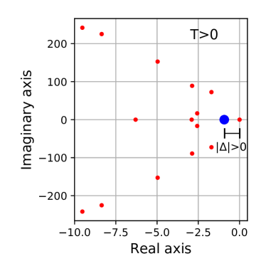
(a) (b)

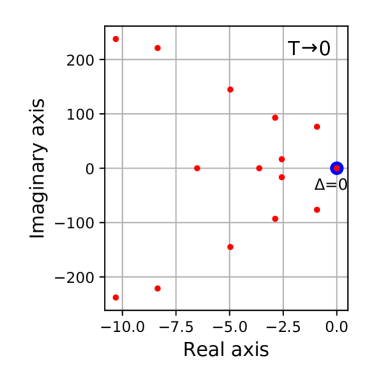
Figure 1: Numerical plots for the distribution of eigenvalues in the real and imaginary axis for two different temperatures. (a) For non-zero temperature, the only one eigenvalue is zero, and $\Delta\neq 0$. The lowest absolute eigenvalue – on the negative real line – is denoted by a large blue marker, whereas other eigenvalues are depicted by small red markers (color online). (b) For $T=0$, we have $\Delta=0$, i.e., the ADR vanishes and we have a frozen non-thermal state.

The quantum phase transition (QPT) occurs when as there is a level crossing between the ground state and the first excited state for some critical value of a suitable parameter Kessler et al. (2012); Sachdev (2011). On the other hand, the DPT is associated with an explicit symmetry breaking, as the degeneracy of the steady-state vanishes by crossing the critical limit Buča and Prosen (2012). The DPT arises when the spectral gap $\Delta$ vanishes Kessler et al. (2012). The Liouvillian is then degenerate. For an ensemble of two spin-system, if there exists a parameter $\alpha$ such that, beyond a critical value of $\alpha$ (say, $\alpha_{c}$), the transition between two different phases takes place. Hence, for $\alpha<\alpha_{c}$, one eigenvalue of $\mathcal{\hat{L}}$ is zero, and for $\alpha\geq\alpha_{c}$, more than one eigenvalues are zero. When $T>0$, the Liouvillian has only one zero eigenvalue state. As the trace is preserved in the whole dynamics, the steady-state dynamics is confined to the observables $\{M_{z},M_{zz}\}$ in the Eq. (7). The steady-state solution is given by,

$$M_{z}|_{t\rightarrow\infty} = M_{\circ}$$

$$M_{zz}|_{t\rightarrow\infty} = M_{\circ}^{2}/4$$ (8)

The steady state density matrices is thermal, $\rho^{ss}_{s}=e^{-\beta(\mathcal{H}^{0}_{1s}+\mathcal{H}^{0}_{1s})}/\mathcal{Z}_{s}$, where $\mathcal{Z}_{s}$ is the partition function of the system. Consequently, the equilibrium magnetization is $M_{\circ}=\tanh(\beta\omega_{\circ}/2)$. On the other hand, for $T=0$, there exist a weak symmetry generator $\hat{D},[S=\sigma_{x}\otimes\sigma_{x}+\sigma_{y}\otimes\sigma_{y}+\sigma_{z}\otimes\sigma_{z}$] and under the unitary transformation [$\hat{U}(t)=\exp(-i\hat{D}t)$]  $\mathcal{L}$ is conserved. Following Noether’s theorem, for every symmetric operation, there exist a conserved quantity Albert and Jiang (2014). Moreover, a symmetry operator $\mathcal{P}$ is strong if it commutes with each of the Lindbladian operators (such as, $\mathcal{O}$ in the Eq. (5)), and is weak if it commutes only with the entire Liouvillian Lieu et al. (2020). From the Eq. (7), we obtain,

$$\frac{d}{dt}\left(M_{c}+M_{zz}\right)=0.$$ (9)

Therefore, the final solution has an initial value dependence. $\mathcal{\hat{L}}$ can be written as a block-diagonal form of the eigenbasis of the superoperator of $\hat{D}$. The steady-state dynamics is confined in the observables-$\{M_{z},M_{zz},M_{c}\}$. The steady state solution is given by,

$$M_{z}|_{t\rightarrow\infty} = M_{\circ}\left[\frac{(4F+3)}{\left(M_{\circ}^{2}+3\right)}\right]$$

$$M_{c}|_{t\rightarrow\infty} = \left[\frac{4F-M_{\circ}^{2}}{2\left(M_{\circ}^{2}+3\right)}\right]$$

$$M_{zz}|_{t\rightarrow\infty} = F-M_{c}$$ (10)

where, $F=(M_{zz}+M_{c})|_{t=0}$. This result is in agreement with earlier work Benatti and Floreanini (2006). The physical meaning of $M_{c}$ can be emphasize in a simpler manner. Using the expression for the steady state concurrence, $C(\rho_{s}^{ss})$, the condition for the persistent entanglement is given by, $4|M_{c}|>\sqrt{(1+4M_{zz})^{2}-4M_{z}^{2}}$ Hill and Wootters (1997). Therefore, if $M_{c}\neq 0$, it signifies there is a possibility of bath-induced persistent entanglement in this phase. We note that the bath induced entanglement (for a common bath) is a well-known concept since the seminal work of Plenio and others Plenio et al. (1999); An et al. (2007); Benatti et al. (2008); Zhang and Yu (2007); Choi and Lee (2007).

The correlation length of the bath is modeled as a monotonic function of the temperature, as mentioned earlier. Since the phase transition happens at $T=0$, we study the observables’ behavior in Eq. (7) as a function of temperature. Figure 2(a-c) depicts the behavior of the observables $\{M_{z},M_{zz},M_{c}\}$ as a function of the time for a set of fixed temperatures. At $T\to 0$ or $\alpha=1$, the expectation value of zero-quantum operator $M_{c}$ remains finite in the steady-state, whereas it vanishes for $T>0$. The existence of $M_{c}\neq 0$ indicates the presence of the persistent entanglement. The vanishing of the entanglement for $T>0$ is in line with the works of Huelga and others, who showed that regular Markovian local environments lead to separable steady-states Huelga et al. (2012). Figures 2(d-f) show the observables’ behavior and their derivatives as a function of the temperature. The temperature has been varied linearly, and $\alpha$ was calculated using the relation between $\xi$ and $\beta$ mentioned earlier. The sudden jump of the observables and the discontinuity of their derivatives clearly show the first-order nature of this DPT.

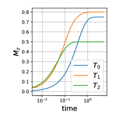
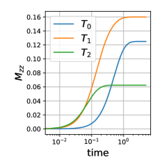
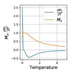
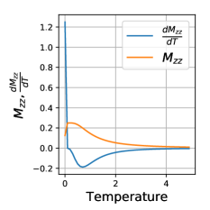
(a) (b) (c)
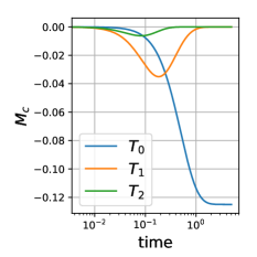
(d) (e) (f)

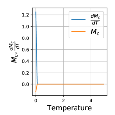
Figure 2: (a), (b) and (c) show the plots of three observables $\{M_{z},M_{zz},M_{c}\}$ as a function of time $(t)$ respectively, obtained by numerically solving Eq. (7), for three choice of $\{R_{1},M_{\circ},\alpha\}$. The parameter sets are chosen as $\{R_{1}=1.0,M_{\circ}=1.0,\alpha=1.0\}$ which correspond to $T=0$ or common bath, the other sets $\{R_{1}=5.0,M_{\circ}=0.8,\alpha=0.5\}$, and $\{R_{1}=10.0,M_{\circ}=0.8,\alpha=0.5\}$ correspond to two non-zero temperatures $T_{1}<T_{2}$. The parameter sets are labeled by $T_{\circ}$ (for $T=0$), $T_{1}$ and $T_{2}$ with colors blue, orange and green, respectively (color online). (a) and (b) shows that the equilibrium values of $M_{z}$ and $M_{zz}$ are less at $T_{2}$ compared to that of at $T_{1}$. For $T_{2}<T_{1}$ the behavior is expected. We note that the $T=0$ behavior shows an anomaly, i.e., $M_{z}|_{T=0}<M_{z}|_{T_{1}}$. (c) $M_{c}$ is non-zero for $\alpha=1$ (i.e., $T=0$) which clearly shows the persistent entanglement, whereas no such persistent entanglement survives at the finite temperatures. (d), (e) and (f) show the steady state value each observable and their temperature derivative versus temperature ($T$). The first order derivatives of all observables diverge at the point $T\to 0$.

Hence, there exist a critical value of $T_{\circ}$ ($T=0$), which is responsible for the symmetry breaking phase transition of the system.

$$\lim_{T\to T_{\circ}}\,\frac{\delta}{\delta T}\text{Tr}[\rho_{s}^{ss}(T)(D)]=\infty$$ (11)

The first order derivative w.r.t $T$ vanishes at $T\to T_{\circ}$. So, it is a first-order phase transition Minganti et al. (2018).

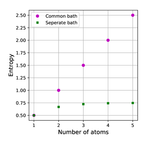
Figure 3: Figure shows the numerical plot of von Neumann entropy from the steady-state density matrix as a function of the number of atoms. To compare the effects of the common environment versus the separate environment, we set $\alpha=1$ (green filled-square markers for common environment) and $\alpha=0.5$ (magenta filled-circle markers for separate environment), while keeping other parameters, constant ($R_{1}=1.0$, and $M_{\circ}=0.6$). It is clear that for the separate environment ($\alpha<1$), the entropy increases following the volume law and hence is linear. On the other hand, for the common environment ($\alpha=1$), the system is frozen and the entropy is no longer an extensive thermodynamic quantity.

We note that since a common environment can exist at a finite temperature Plenio et al. (1999), hence such phases do not strictly require one to reach zero temperature. Multiple ions have been confined in a common electromagnetic field at a finite temperature using the trapped-ion technique Wineland and Itano (2008); Poyatos et al. (1996a). Hence, for a longer bath-correlation length $(\xi)$, we can make $\alpha\to 1$ at a sufficiently low temperature.

We show here a comparative study of change of the von Neumann entropy $(\mathcal{S}=-Tr_{s}\{\rho_{s}\ln\rho_{s}\})$ by increasing the number of atoms in a common bath and separate bath, in figure 3. The entropy is extensive for the separate local environments and increases linearly with the number of constituent atoms ($n$). But for common environments, one expects an area law obtained from the derivative of the volume law with respect to $n$ and hence the entropy should be independent of $n$ Eisert et al. (2010). We simulate the $n$ TLS, keeping them connected to a common environment. The switch over from the volume law to the area law is shown in Fig. 3. Corresponding dark state, in terms of observables, can be calculated by putting $F=-3/4$, we get $M_{z}=0$ and $M_{c}=-1/2$, $M_{zz}=-1/4$. The steady-state is temperature independent, and also it is a pure state. The wave function of the dark state is, $|\psi\rangle=\frac{1}{\sqrt{2}}(|01\rangle-|10\rangle)$, a singlet state between the two spins. With the addition of other spins, such states are found for each pair of spins. An addition of another spin results in a set of dark states. Upon further addition of spins, the entropy does not increase anymore (only the dark states are created).

IV Conclusion

We identify a spatially-correlated bath as a completely common environment in the zero-temperature limit. The same environment acts as a regular local environment with non-zero temperatures. Several conserved quantities can be identified when non-interacting systems are in a common environment. Hence persistent entanglement exists under this dissipative dynamics. Increasing the number of spins, the number of integrability also increases. On the other hand, the presence of separately local environments ensures that the system is non-integrable. Hence, the system evolves to a thermal state after a sufficiently long time. There exist a temperature-driven first-order phase transition. At the critical limit ${T\to 0}$, a weak symmetry characterizes the final steady-state, the system skips thermalization. We note that recent laser-cooled ion-trap experiments set a major goal to observe this effect at a finite temperature Poyatos et al. (1996b); Wilson-Rae et al. (2004); Sarlette et al. (2011); Tomadin et al. (2012); Stellmer et al. (2013).