A polarization tensor approximation for the Hessian in iterative solvers for non-linear inverse problems

Abstract

For many inverse parameter problems for partial differential equations in which the domain contains only well-separated objects, an asymptotic solution to the forward problem involving ‘polarization tensors’ exists. These are functions of the size and material contrast of inclusions, thereby describing the saturation component of the non-linearity. As such, these asymptotic expansions can allow fast and stable reconstruction of small isolated objects. In this paper, we show how such an asymptotic series can be applied to non-linear least-squares reconstruction problems, by deriving an approximate diagonal Hessian matrix for the data misfit term.

Often, the Hessian matrix can play a vital role in dealing with the non-linearity, generating good update directions which accelerate the solution towards a global minimum which may lie in a long curved valley, but computational cost can make direct calculation infeasible. Since the polarization tensor approximation assumes sufficient separation between inclusions, our approximate Hessian does not account for non-linearity in the form of lack of superposition in the inverse problem. It does however account for the non-linear saturation of the change in the data with increasing material contrast. We therefore propose to use it as an initial Hessian for quasi-Newton schemes.

This is demonstrated for the case of electrical impedance tomography in numerical experimentation, but could be applied to any other problem which has an equivalent asymptotic expansion. We present numerical experimentation into the accuracy and reconstruction performance of the approximate Hessian, providing a proof of principle of the reconstruction scheme.

1 Introduction

There are two types of non-linearity in inverse parameter problems for boundary value partial differential equations (PDEs) which are observed by practitioners: lack of superposition in measurements due to multiple nearby objects; and saturation of the change in data with increasing material contrast. These two phenomena can be observed in Figure 1, for the case of electrical impedance tomography (EIT). For several PDEs in which the domain contains small well-isolated objects, a solution to the forward problem exists in the form of an asymptotic expansion involving generalised polarization tensors (GPTs), also referred to as ‘polarizability’ tensors; see for example Ammari et al[2]. The terms of such series are in increasing order with respect to the size of inclusion, and with GPTs that are increasingly higher rank tensors. Such asymptotic approximations exist for Maxwell’s equations, metal detection, EIT, acoustics and elasticity, see for example [3, 4, 5, 6, 2, 7, 8]. The polarization tensors depend on the physical regime, but in each case are a function of the shape of inclusions and material contrast. The use of such models to solve the inverse problem can then deal well with non-linearity due to material contrast. In general they provide no information about the lack of superposition, due to assuming sufficiently separated objects.

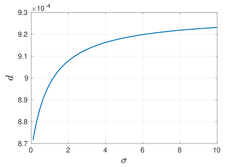
(a) Saturation of a single datum $\mathrm{d}$ over material contrast $\sigma$.

(b) Deviation from superposition effect with separation distance between the boundaries of two inclusions.

Figure 1: Two types of non-linearity observed in inverse boundary-value problems for PDEs, in the case of EIT. (a) Saturation of a datum $d$ with material contrast of a single inclusion. (b) Lack of linear superposition, $\|\mathbf{d}^{\prime}_{\mathrm{both}}-(\mathbf{d}^{\prime}_{1}+\mathbf{d}^{\prime}_{2})\|_{2}/\|\mathbf{d}^{\prime}_{\mathrm{both}}\|_{2}$ against the separation distance between the boundary of two inclusions. $\mathbf{d}^{\prime}_{\mathrm{both}}$ is the change in data from a homogeneous domain with two inclusions, $\mathbf{d}^{\prime}_{1}$ and $\mathbf{d}^{\prime}_{2}$ the change in data with the first and second inclusion alone, respectively.

Where the inverse problem does not only involve well isolated objects, one often attempts to solve numerically the more generic (possibly large-scale or high-dimensional) non-linear least-squares reconstruction problem

$$\mathbf{m}_{\mathrm{im}}=\operatorname*{argmin}_{\mathbf{m}\in M}\|\mathcal{F}(\mathbf{m})-\mathbf{d}\|_{2}^{2}+\lambda R(\mathbf{m}),$$ (1.1)

where $\mathbf{m}\in M\subseteq\mathds{R}^{N_{m}}$ is a discretisation of physical parameters to be recovered, $\mathbf{m}_{\mathrm{im}}$ the reconstructed parameters (or image), $\mathbf{d}\in\mathds{R}^{N_{d}}$ the observed data, and $\mathcal{F}:\mathds{R}^{N_{m}}\rightarrow\mathds{R}^{N_{d}}$ is the forward operator simulating data. Prior knowledge is incorporated through the regularisation term $R:\mathds{R}^{N_{m}}\rightarrow\mathds{R}^{+}$, which stabilises ill-conditioned and over- or under-determined inverse problems, effectively preventing over-solving and fitting noise, with regularisation parameter $\lambda>0$; see for example Tarantola[9] or Vogel[10]. Solving this problem can have a high computational cost, since iterative solution involves calculating $\mathcal{F}(\mathbf{m}^{[k]})$ for many different iterates $\mathbf{m}^{[k]}$ (the forward problem). Both lack of superposition and saturation must be dealt with by the reconstruction scheme.

Due to both non-linearity and ill-posedness, the topography of the cost function is often characterised by an elongated curved valley, as well as having multiple local minima[11]. The Hessian matrix of the least-squares data-misfit function can play an important role in dealing with these features of (1.1). It describes parameter illumination in the data, interactions between two nearby inclusions in off-diagonal terms, and the non-linear saturation effect in the leading diagonal – to second order. Incorporating the Hessian (or an approximation) in a Newton-type method therefore acts to refocus the gradient direction[12, 13, 14, 15, 16], often arriving more rapidly towards the minimum of the valley. However, calculation of this large and possibly dense matrix in full is not always possible due to memory and computation time constraints. Several alternative approaches may be taken to efficiently incorporate information from the Hessian in the update direction without calculating it directly. These include Gauss-Newton[17, 18], quasi-Newton [13, 19, 20], and inexact Newton methods[21, 22, 23], to reference a few.

In this paper, we use a polarization tensor approximation (specifically, the classical Pólya-Szegö tensor) to derive an approximate diagonal of the Hessian matrix, which is computationally very cheap compared with calculating the true diagonal. We propose to use this as an initial Hessian estimate in quasi-Newton schemes in a novel ‘mixed-model’ approach. We investigate the effectiveness of encoding information about the non-linear saturation as well as parameter illumination into the reconstruction scheme in this way. This approach is widely applicable to any inverse parameter problem for boundary value PDEs for which such an asymptotic expansion exists.

To demonstrate the method we apply it to the EIT reconstruction problem. This is both severely ill-posed and non-linear and so provides a sufficiently challenging test of the method. We provide numerical evidence of the performance of the method, both in terms of the quality and efficiency of the reconstruction, as well as how accurate an approximation to the true Hessian we have. The results presented are for 2D reconstruction problems, but it is large-scale inverse problems, where memory is a limiting factor, for which we expect most utility to be gained. Previously, we have also used this method for 3D reconstruction of ground-penetrating radar data[24, 25]. Thus, we provide a proof of principle for the method to be used for large scale non-linear inverse problems in general.

This paper is organised as follows. In Section 2, we outline the theoretical background to EIT, which is the physical problem we will use to demonstrate the reconstruction method. In Section 3, we cover the relevant literature results on asymptotic solution to the generalised Laplace equation in terms of polarization tensors, as well as properties of the classical tensor of Pólya and Szegö. In Section 4 we discuss reconstruction schemes, and in particular Section 4.1 uses the asymptotic approximation of Section 3 to derive the approximate diagonal Hessian matrix which we propose to use as an initial Hessian approximation in l-BFGS. Finally, numerical experimentation and discussion of the results is presented in Section 5. This includes both qualitative and quantitative comparison of the approximate Hessian to the true one, as well as reconstruction results using the approximate Hessian initialised l-BFGS scheme.

2 Electrical Impedance Tomography

The aim of EIT is to reconstruct the conductivity of an object from low-frequency electrical measurements obtained on the boundary. In the zero frequency limit, the relationship between the electrical potential, $u$, and conductivity, $\sigma$, is governed by a second order, linear PDE

$$\left\{\begin{array}[]{l}\nabla\cdot\left(\sigma\nabla u\right)=0\quad x\in\Omega\subset\mathds{R}^{d}\\ \left.\sigma\frac{\partial u}{\partial\nu}\right|_{\partial\Omega}=g\end{array}\right.$$ (2.1)

where the domain $\Omega$ has boundary $\partial\Omega$ and $d=2,3$. In general $\sigma$ can be anisotropic but in this paper we will consider isotropic conductivity $\sigma:\Omega\to\mathds{R}$, bounded above and below, $0<c<\sigma(x)<C$ almost everywhere for constants $c,C\in\mathds{R}$, denoted $\sigma\in L^{\infty}_{+}(\Omega)$. Given Neumann boundary conditions i.e. $\sigma\frac{\partial u}{\partial\nu}|_{\partial\Omega}=g$, $g\in H^{-\frac{1}{2}}(\partial\Omega)$, (2.1) has a unique weak solution $u\in H^{1}(\Omega)/\mathds{R}$, where the quotient space reflects that the electric potential is only defined up to a constant. We denote the Neumann-to-Dirichlet map $\Lambda_{\sigma}:H^{-\frac{1}{2}}(\partial\Omega)\to H^{\frac{1}{2}}(\partial\Omega)$ as

$$\Lambda_{\sigma}(g)=u|_{\partial\Omega}.$$ (2.2)

The mathematical formulation of the inverse conductivity problem is then to study the determination of $\sigma$ from $\Lambda_{\sigma}$. This problem is non-linear and severely ill-posed, and in practice one only has partial knowledge of the boundary data, $\Lambda_{\sigma}$, which is subject to measurement noise (see e.g. [26, 27, 28] for review articles on reconstruction algorithms and theoretical results for EIT).

2.1 EIT forward modelling

In practice only a finite number of currents and voltage measurements can be applied and measured respectively and on finite sized electrodes, and in many applications there is a power drop due to formation of contact impedance at electrode/domain interfaces. We consider $N_{L}$ electrodes and denote with $E_{l}\subset\partial\Omega$ the subset of boundary in contact with the $l^{th}$ electrode and $E_{T}^{{}^{\prime}}:=\partial\Omega\setminus\bigcup_{l=1}^{N_{L}}E_{l}$. The complete electrode model (CEM) [29] consists of the conductivity equation (2.1) along with the boundary conditions

$$(u+\eta_{l}\sigma\frac{\partial u}{\partial\nu})|_{E_{l}}=U_{l},\hskip 8.53581ptl=1,\ldots,L,\hskip 17.07164pt\sigma\frac{\partial u}{\partial\nu}=0,\hskip 8.53581ptx\in E_{T}^{{}^{\prime}},\hskip 17.07164pt\int_{E_{l}}\sigma\frac{\partial u}{\partial\nu}\,\mathrm{d}s=I_{l},$$ (2.3)

where $I:=(I_{1},\ldots,I_{N_{L}})^{T}\in\mathds{R}^{N_{L}}$, with $\sum_{l=1}^{N_{L}}I_{l}=0$, are the inflow currents, $\eta:=(\eta_{1},\ldots,\eta_{N_{L}})^{T}\in\mathds{R}^{N_{L}}$ are the contact impedances and $U:=(U_{1},\ldots,U_{N_{L}})^{T}\in\mathds{R}^{N_{L}}$ are the potentials. The CEM forward problem is then: given $\sigma$ and $I$, determine $u$ and $U$. There is a unique weak solution $(u,U)\in(H^{1}(\Omega)\oplus\mathds{R}^{N_{L}})/\mathds{R}$ to this problem [29].

We now discuss a numerical solution to the CEM forward problem using the finite element method (FEM) (for further details on FEM see e.g. [30, 31, 32, 33, 34, 35]). In the FEM the domain $\Omega$ is decomposed into $N_{E}$ disjoint elements $\{\Omega_{i}\}_{i=1}^{N_{E}}$, chosen here to be triangles, with $\Omega=\cup_{i=1}^{N_{E}}\Omega_{i}$, joined at $N_{N}$ vertex nodes $\{x_{i}\}_{i=1}^{N_{N}}$. A piecewise constant conductivity discretisation, $\sigma=\sum_{i=1}^{N_{E}}m_{i}\chi_{i}$, is chosen here where $\chi_{i}$ is the characteristic function of $\Omega_{i}$ and ${\mathbf{m}}:=(\mathrm{m}_{1},\ldots,\mathrm{m}_{N_{E}})^{T}\in\mathds{R}^{N_{E}}$ is the representation of the conductivity. In the FEM, a continuous approximation to the weak solution of (2.1), $u_{h}$, is sought where $u\approx u_{h}=\sum_{i=1}^{N_{N}}\upalpha_{i}\psi_{i}$, where $\upalpha:=(\upalpha_{1},\ldots,\upalpha_{N_{N}})^{T}\in\mathds{R}^{N_{N}}$ and $\{\psi_{i}\}_{i=1}^{N_{N}}$ are the shape functions, chosen here to be piecewise linear. Additionally, an approximation $\upbeta:=(\upbeta_{1},\ldots,\upbeta_{N_{L}})^{T}\in\mathds{R}^{N_{L}}$ to the electrode potentials is sought such that $U\approx\upbeta$. As described by Vauhkonen [33, pg. 44], $(\upalpha,\upbeta)$ is given by the solution of the system of equations

$$\mathrm{S}(\mathbf{m})\left(\begin{array}[]{c}\mathbf{\upalpha}\\ \vskip 6.0pt plus 2.0pt minus 2.0pt\cr\mathbf{\upbeta}\end{array}\right):=\left(\begin{array}[]{cc}\mathrm{A}(\mathbf{m})+\mathrm{B}&\mathrm{P}\\ \vskip 6.0pt plus 2.0pt minus 2.0pt\cr\mathrm{P}^{T}&\mathrm{Q}\end{array}\right)\left(\begin{array}[]{c}\mathbf{\upalpha}\\ \vskip 6.0pt plus 2.0pt minus 2.0pt\cr\mathbf{\upbeta}\end{array}\right)=\left(\begin{array}[]{c}\mathrm{0}\\ \vskip 6.0pt plus 2.0pt minus 2.0pt\cr\mathrm{I}\end{array}\right),$$ (2.12)

where the stiffness matrix $\mathrm{A}(\mathbf{m})$ is given by

$$\mathrm{A}_{ij}:=\int_{\Omega}(\sigma\nabla\psi_{i})\cdot\nabla\psi_{j}\,\mathrm{d}\Omega,\hskip 11.38109pti,j=1,\ldots,N_{N},$$ (2.13)

and the matrices $\mathrm{B}$, $\mathrm{P}$ and $\mathrm{Q}$ by

$$\mathrm{B}_{ij}:=\sum_{l=1}^{N_{L}}\frac{1}{\eta_{l}}\int_{E_{l}}\psi_{i}\psi_{j}\,\mathrm{d}s,\hskip 8.53581pt\mathrm{P}_{jl}:=-\frac{1}{\eta_{l}}\int_{E_{l}}\psi_{j}\,\mathrm{d}s,\hskip 8.53581pt\mathrm{Q}_{ll}:=\frac{|E_{l}|}{\eta_{l}},$$ (2.14)

$$i,j=1,\ldots,N_{N},\hskip 8.53581ptl=1,\ldots,N_{L}.$$

This can be written compactly as

$$\mathrm{S}(\mathbf{m})\mathbf{u}=\mathbf{h}$$ (2.15)

where $\mathbf{u}:=(\mathbf{\upalpha},\mathbf{\upbeta})^{T}$, $\mathbf{h}:=(\mathbf{0},\mathbf{I})^{T}$. The potential $\mathbf{u}$ is only defined up to a constant resulting in a $1$-dimensional null space of $S$, but this problem is resolved by choosing an interior node, with coordinate $x_{c}$, to be at zero potential $\mathbf{u}(x_{c})=\mathbf{0}$. The $c^{th}$ row and column of $\mathrm{S}$ and $c^{th}$ row of $\mathbf{u}$ and $\mathbf{h}$ are removed to generate $\tilde{\mathrm{S}}$, $\tilde{\mathbf{u}}$ and $\tilde{\mathbf{h}}$, and an $N_{N}+N_{L}-1$ dimensional linear system $\tilde{\mathrm{S}}(\mathbf{m})\tilde{\mathbf{u}}=\tilde{\mathbf{h}}$ is solved for $\tilde{\mathbf{u}}$.

The forward problem is solved with $N_{L}-1$ right hand side vectors $\{\tilde{\mathbf{h}}^{[n]}\}_{n=1}^{N_{L}-1}$, that are determined from $N_{L}-1$ linearly independent current vectors $\{I^{[n]}\}_{n=1}^{N_{L}-1}$, yielding solutions $\tilde{\mathbf{u}}^{[n]}=\tilde{\mathrm{S}}(\mathbf{m})^{-1}\tilde{\mathbf{h}}^{[n]}$ and measured voltage patterns $U^{[n]}$, $n=1,\ldots,N_{L}-1$. We define the $r$^th measurement as the voltage difference between electrode $l$ and electrode $(l\operatorname{mod}N_{L})+1$ at the application of the $n$^th current, $U^{[n]}_{(l\operatorname{mod}N_{L})+1}-U^{[n]}_{l}$, $l=1,\ldots,N_{L}$, and $r=N_{L}(n-1)+l$. This can be written using a linear measurement operator $\mathbf{t}^{[l]}$ (a column vector) that generates the $r$^th component of simulated data, $\mathrm{f}_{r}$, through $\mathrm{f}_{r}:=(\mathbf{t}^{[l]})^{T}\tilde{\mathbf{u}}^{[n]}$, and $\mathcal{F}(\mathbf{m})=[\mathrm{f}_{1},\ldots,\mathrm{f}_{N_{d}}]^{T}$. This results in $N_{d}=\frac{1}{2}N_{L}(N_{L}-1)$ independent measurements (with a factor of $\frac{1}{2}$ accounting for redundancy in measurements due to $\Lambda_{\sigma}$ being self-adjoint, $\Lambda_{\sigma}=\Lambda_{\sigma}^{*}$). Hereon, the tilde notation for the modified system will be dropped, and it is understood that we are using the modified system.

3 Generalized Polarization tensors

In this section, we provide some background results on generalized polarization tensors from the literature, for the expression we will make use of for our Hessian approximation. For further details, see Ammari and Kang[36] and others[37, 38, 5, 4, 6, 3, 7, 2].

We wish to describe the effect on the electric potential of a single inclusion in domain $\Omega$ via an asymptotic expansion. Let $B\subset\Omega\subset\mathds{R}^{d}$ (the inclusion) be a bounded domain containing the point $z$. Let the conductivity of $B$ be $\gamma$, where $0<\gamma\neq 1$, with the conductivity of the background equal to $1$ so that $\gamma$ is the ratio between conductivity of the object and conductivity of the background. The conductivity is thus

$$\sigma=1+(\gamma-1)\chi(B),$$ (3.1)

where $\chi(B)$ is the characteristic function of $B$. Denote by $u_{0}$ the field in the absence of the object i.e. the solution of (2.1) with $\sigma\equiv 1$, and let $u$ the perturbed field which is the solution of (2.1) with $\sigma$ given as in (3.1). For $B$ sufficiently far from $\partial\Omega$, the perturbation in electric field satisfies the asymptotic formulae[37, 36]

$$\Lambda_{D}(g)(x)-\Lambda_{0}(g)(x)=-\epsilon^{d}\nabla u_{0}(z)\mathcal{M}\nabla_{z}N(x,z)+\mathcal{O}(\epsilon^{d+1})$$ (3.2)

as $\epsilon\rightarrow 0$, where $\epsilon$ is the size (diameter) of the inclusion, $\Lambda_{D}$ and $\Lambda_{0}$ are the Neumann-to-Dirichlet maps $\Lambda_{D}(g)=u|_{\partial\Omega}$ and $\Lambda_{0}(g)=u_{0}|_{\partial\Omega}$, respectively, and $N$ is the Neumann function satisfying

$$\left\{\begin{array}[]{l}\nabla^{2}_{x}N(x,z)=-\delta(x-z)\quad\mbox{in }\Omega,\\ \left.\frac{\partial N}{\partial\nu_{x}}\right|_{\partial\Omega}=-\frac{1}{|\partial\Omega|},\\ \int_{\partial\Omega}N(x,z)\,\mathrm{d}s(x)=0,\end{array}\right.$$ (3.3)

where $\delta$ is the Dirac delta distribution. The first-order polarization tensor $\mathcal{M}$ is the classical Pólya-Szegö tensor associated with $B$. It varies with the conductivity contrast of the inclusion $\gamma$ as well as its shape $B$, but not with the position of the inclusion $z$. This tensor can be explicitly computed for disks and ellipses in the plane, as well as balls and ellipsoids in three-dimensional space. For example, if $B$ is an ellipse whose semi-axes of length $a$ and $b$ are on the $x_{1}$– and $x_{2}$– axis and, respectively, then its Pólya-Szegö tensor $\mathcal{M}$ can be written in matrix form as

$$\mathcal{M}=(\gamma-1)|B|\begin{bmatrix}\frac{a+b}{a+\gamma b}&0\\ 0&\frac{a+b}{b+\gamma a}\end{bmatrix},$$ (3.4)

where $|B|$ denotes the volume of $B$. Moreover, the change in tensor owing to a unitary transformation of the inclusion can also be readily computed. If $B^{\prime}\subset\Omega$ is a rotation of the ellipse $B$ such that it is not oriented with the coordinate axes, the first-order polarization tensors $\mathcal{M}$ and $\mathcal{M}^{\prime}$ associated with $B$ and $B^{\prime}$ (respectively) are related by[38]

$$\mathcal{M}=\mathrm{R}\mathcal{M}^{\prime}\mathrm{R}^{T},$$ (3.5)

where $\mathrm{R}$ is the rotation matrix from the coordinate axes to the principle axes of $B^{\prime}$.

Remark 3.1.

For any given Pólya-Szegö tensor $\mathcal{M}$, an elliptical (in 2D) or an ellipsoidal (in 3D) inclusion can be constructed with the same tensor. We need only construct a tensor with the correct eigenvalues via (3.4), to which we apply a unitary transformation matrix $R$ as in (3.5) to align the eigenvectors. Effectively, this tells us that the most this second rank tensor tells us about the effect of an inclusion on a field, is the effect of its closest fitting oriented ellipse/ellipsoid would have on that field (to first order), see e.g. [39, 4].

Equation (3.2) can be extended to the case of a domain containing multiple inclusions $B_{1},\ldots,B_{m}$, sufficiently separated from both the boundary and one-another, by

$$\Lambda_{D}(g)(x)-\Lambda_{0}(g)(x)=-\sum_{s=1}^{m}\epsilon^{d}_{s}\nabla u_{0}(z_{s})\mathcal{M}^{(s)}\nabla_{z}N(x,z_{s})+\mathcal{O}(\epsilon^{d+1})$$ (3.6)

as $\epsilon\rightarrow 0$, where $\mathcal{M}^{(s)}$ and $z_{s}$ are the polarization tensor and centre of the inclusion $B_{s}$. Equation (3.6) is also the first term in a full asymptotic series[38, pg. 29, thm 4.1]

$$\Lambda_{D}(g)(x)-\Lambda_{0}(g)(x)=-\sum_{s=1}^{m}\sum_{|\alpha|,|\beta|=1}^{d}\frac{\epsilon^{|\alpha|+|\beta|+d-2}}{\alpha!\beta!}(\partial^{\alpha}u_{0})(z_{s})\partial_{z}^{\beta}N(x,z_{s})\mathscr{M}_{\alpha\beta}^{(s)}+\mathcal{O}(\epsilon^{2d})$$ (3.7)

as $\epsilon\rightarrow 0$, for multi-indices $\alpha,\beta$ and a common (largest) length scale of inclusions $\epsilon$. Here the Pólya-Szegö tensors $\mathcal{M}^{(s)}0$ are replaced by Generalised Polarization Tensors (GPTs) $\mathscr{M}_{\alpha\beta}^{(s)}$, with the first order GPTs (for $|\alpha|=|\beta|=1$) being $\mathcal{M}^{(s)}$. The GPTs can be calculated by carrying out boundary integrals about the inclusion shapes $B_{s}$ of an auxiliary field from a surrogate transmission problem, as well as other equivalent formulae[2, 38]. They can also be calculated for inhomogeneous inclusions, i.e. providing a single GPT which can be used to describe the field perturbed by multiple nearby (or touching) inclusions. The formulae are not needed for the purpose of this paper, but note that the components of the GPTs themselves depend only on $\gamma$ and $B_{s}$, and not on the incident field $u_{0}$ or the position of the object $z$.

The GPTs therefore provide a way to describe the change in electric field due to the shape and conductivity of a set of inclusions, separating these properties of the inclusions from the incident field. An equivalent expression exists for the free-space problem, in which the Neumann function $N$ is replaced by the free-space Green’s function[38]. Equivalent asymptotic expansions involving GPTs for other physical modalities, with different formulae for the associated GPTs[36].

In (3.7) higher order terms involve derivatives of the incident field $u_{0}$ and measurement (adjoint) field $N$. So for incident fields which are fairly uniform these terms quickly become negligible, as well as the series converging rapidly with decreasing size of inclusions. The same holds true for the measurement (adjoint) field, by reciprocity. This tells us that to be sensitive to an object’s shape – beyond finding the closest fitting ellipsoid – we must use source and adjoint fields which are non-uniform.

The Hessian approximation which we later propose will make use of the first term in the asymptotic series, namely equation (3.6), as well as explicit formulae for the Pólya-Szegö tensor $\mathcal{M}$. If further explicit formulae were developed for higher order terms or differently shaped inclusions, these could readily be used also.

Neumann function computation

For some domains an analytic solution is available for the Neumann function. For example, for $\Omega$ a disc of radius $\rho$ it is given by[36, pg. 44, eq. 2.58]

$$N(x,z)=-\frac{1}{2\pi}\Big{(}\ln|x-z|+\ln\Big{|}\frac{\rho}{|x|}x-\frac{|x|}{\rho}z\Big{|}+\frac{\ln\rho}{\pi}\Big{)}.$$ (3.8)

Note that $N$ will be well-defined for the purposes of (3.6), which always has $x\in\partial\Omega$ and $z\in\Omega$ sufficiently separated from $\partial\Omega$ (so that $z\neq x$).

For more general domain shapes for which there is no analytic solution available one can instead use a numerical approximation to the Neumann function, and we now describe a finite element approximation to this. We seek $N_{N}$ continuous finite element approximations to $\{N(x,z_{k})\}_{k=1}^{N_{N}}$, $N_{h}^{(k)}=\sum_{i=1}^{N_{N}}\mathrm{\Upgamma}_{i}^{(k)}\psi_{i}$, where the $k\textsuperscript{th}$ approximation corresponds to a delta function source supported at node $k$, and $\mathrm{\Upgamma}\in\mathds{R}^{N_{N}\times N_{N}}$ with the $k\textsuperscript{th}$ column representing the approximation to $N(x,z_{k})$. The weak formulation for (3.3), in conjunction with this approximation, leads to the system of equations

$$\left(\begin{array}[]{c}\mathrm{A}\\ \vskip 6.0pt plus 2.0pt minus 2.0pt\cr\mathrm{F}\end{array}\right)\mathrm{\Upgamma}=\left(\begin{array}[]{c}\mathrm{G}\\ \vskip 6.0pt plus 2.0pt minus 2.0pt\cr\mathrm{0}\end{array}\right),$$ (3.9)

where $\mathrm{A}\in\mathds{R}^{N_{N}\times N_{N}}$ is the stiffness matrix (2.13) with $\sigma=1$, and $\mathrm{F}\in\mathds{R}^{1\times N_{N}}$ and $\mathrm{G}\in\mathds{R}^{N_{N}\times N_{N}}$ have entries

$$\mathrm{F}_{i}=\int_{\partial\Omega}\psi_{i}\,\mathrm{d}s,\hskip 11.38109pt\mathrm{G}_{ij}=\delta_{ij}-\int_{\partial\Omega}\frac{1}{|\partial\Omega|}\psi_{i}\,\mathrm{d}s\hskip 11.38109pti,j=1,\ldots,N_{N}.$$ (3.10)

where $\delta_{ij}$ is the Kronecker delta. The system (3.9) has full column rank, and we can compute the solution through the normal equations. We note that in two dimensions a delta function has regularity $\delta\in H^{-1-\epsilon}(\Omega)$ for all $\epsilon>0$, and the resulting Neumann function $N(\cdot,z)$, for a source supported at point $z$, will have regularity $N(\cdot,z)\in H^{1-\epsilon}(\Omega)$ for all $\epsilon>0$ falling just short of $H^{1}$-regularity required to guarantee of FE approximation. However, by elliptic regularity, $N(\cdot,z)$ will be smooth ($C^{\infty}$) in complement of any open set containing $z$, and the FE approximation will converge away from each source [35].

For the numerical results presented in Section 5 we use the above analytic Neumann function. For reconstruction problems in domain shapes which do not have an analytic Neumann function, one could numerically compute and store the Neumann function once.

4 The reconstruction scheme

In this section, we provide a brief overview of the numerical solution of the inverse problem with Newton-type methods, including calculation of the gradient and Hessian via the adjoint state method. We then derive our approximate diagonal Hessian matrix, making use of the asymptotic approximation of Section 3, and describe how it can be used in a quasi-Newton method as a part of our “mixed model” approach.

We consider only the least-squares data misfit part of the objective function

$$\mathcal{J}(\mathbf{m}):=\frac{1}{2}\|\mathcal{F}(\mathbf{m})-\mathbf{d}\|_{2}^{2},$$ (4.1)

and recall from Section 2.1 that each component $\mathrm{f}_{r}$ of simulated data $\mathcal{F}(\mathbf{m})=[\mathrm{f}_{1},\ldots,\mathrm{f}_{N_{d}}]^{T}$ involves simulating a datum by solving (2.15) for different boundary conditions. Ignoring for now the omitted regularisation term, we wish to minimise (4.1) using a Newton-type method, which has an update direction given by

$$\mathrm{B}^{[k]}\mathbf{p}^{[k]}=-\nabla\mathcal{J}(\mathbf{m}^{[k]})=:-\mathbf{g}^{[k]},$$ (4.2)

for $\mathrm{B}^{[k]}$ some approximation to the true Hessian $\mathrm{H}^{[k]}:=\nabla_{\mathbf{m}}^{2}\mathcal{J}(\mathbf{m}^{[k]})$, and gradient $\mathbf{g}^{[k]}:=\nabla_{\mathbf{m}}\mathcal{J}(\mathbf{m}^{[k]})$. Dropping the superscript-$[k]$ notation, formally computing the components of the gradient and Hessian yields

$$\mathrm{g}_{j}=\sum_{r=1}^{N_{d}}\mathrm{J}_{rj}\left(\mathrm{f}_{r}-\mathrm{d}_{r}\right),$$ (4.3)

and

$$\mathrm{H}_{ij}=\sum_{r=1}^{N_{d}}\left\{\frac{\partial\mathrm{f}_{r}}{\partial\mathrm{m}_{i}}\frac{\partial\mathrm{f}_{r}}{\partial\mathrm{m}_{j}}+\frac{\partial^{2}\mathrm{f}_{r}}{\partial\mathrm{m}_{i}\partial\mathrm{m}_{j}}\left(\mathrm{f}_{r}-\mathrm{d}_{r}\right)\right\},$$ (4.4)

respectively, where $\mathrm{J}_{rj}=\frac{\partial\mathrm{f}_{r}}{\partial\mathrm{m}_{j}}$ are elements of the Jacobian matrix $\mathrm{J}$, $\mathrm{f}_{r}$ the $r$^th component of simulated data, $\mathcal{F}(\mathbf{m})=[\mathrm{f}_{1},\ldots,\mathrm{f}_{N_{d}}]^{T}$, and $\mathrm{d}_{r}$ the $r$^th component of $\mathbf{d}$.

4.1 Classical adjoint field formulation

In solving the inverse problem, these derivatives are often calculated via an adjoint field formulation (see e.g. [12, 40]). In the continuous setting the EIT forward problem, the map $\mathrm{F}:L^{\infty}(\Omega)\to\mathcal{L}(H^{-\frac{1}{2}}(\partial\Omega),H^{\frac{1}{2}}(\partial\Omega)),\hskip 2.84526pt\sigma\mapsto\Lambda_{\sigma}$, is Fréchet differentiable with respect to $L^{\infty}$ conductivity perturbations up to arbitrary order (see e.g. [41, 42]). The 1st and 2nd Fréchet derivatives of $\mathrm{F}$ at $\sigma\in L^{\infty}(\Omega)$ in the directions $h_{1},h_{2}\in L^{\infty}(\Omega)$ are given by

$$D\mathrm{F}({\sigma}):L^{\infty}(\Omega)\to\mathcal{L}(H^{-\frac{1}{2}}(\partial\Omega),H^{\frac{1}{2}}(\partial\Omega)),\hskip 2.84526pth_{1}\mapsto D\Lambda_{\sigma}[h_{1}],$$ (4.5)

$$D^{2}\mathrm{F}({\sigma}):L^{\infty}(\Omega)\times L^{\infty}(\Omega)\to\mathcal{L}(H^{-\frac{1}{2}}(\partial\Omega),H^{\frac{1}{2}}(\partial\Omega)),\hskip 2.84526pt(h_{1},h_{2})\mapsto D^{2}\Lambda_{\sigma}[h_{1},h_{2}],$$ (4.6)

where $D\Lambda_{\sigma}[h_{1}](g)=\delta u|_{\partial\Omega}$ and $D^{2}\Lambda_{\sigma}[h_{1},h_{2}](g)=\delta^{2}u|_{\partial\Omega}$, with $\delta u$ and $\delta^{2}u$ given by

$$\nabla\cdot(\sigma\nabla\delta u)=-\nabla\cdot(h_{1}\nabla u),\hskip 11.38109pt \left.\sigma\frac{\partial\delta u}{\partial\nu}\right|_{\partial\Omega}=0,$$ (4.7)

$$\nabla\cdot(\sigma\nabla\delta^{2}u)=-\nabla\cdot(h_{2}\nabla\delta u),\hskip 11.38109pt \left.\sigma\frac{\partial\delta^{2}u}{\partial\nu}\right|_{\partial\Omega}=0,$$ (4.8)

$u$ is the solution to the forward problem (2.1), and by definition

$$\int_{\partial\Omega}g^{*}(\Lambda_{\sigma+h_{1}}(g)-\Lambda_{\sigma}(g))\,\mathrm{d}s=\int_{\partial\Omega}g^{*}D\Lambda_{\sigma}[h_{1}](g)\,\mathrm{d}s+o(||h_{1}||_{L^{\infty}}),$$ (4.9)

$$\int_{\partial\Omega}g^{*}(D\Lambda_{\sigma+h_{2}}[h_{1}](g))-D\Lambda_{\sigma}[h_{1}](g))\,\mathrm{d}s=\int_{\partial\Omega}g^{*}D^{2}\Lambda_{\sigma}[h_{1},h_{2}](g)\,\mathrm{d}s+o(||h_{2}||_{L^{\infty}}).$$ (4.10)

Further, efficient, adjoint-field formulae for the 1st and 2nd Fréchet derivatives at $\sigma$ are given by

$$\int_{\partial\Omega}g^{*}(D\Lambda_{\sigma}[h_{1}](g))\,\mathrm{d}s=-\int_{\Omega}h_{1}\nabla u^{*}\cdot\nabla u\,\mathrm{d}\Omega,$$ (4.11)

$$\int_{\partial\Omega}g^{*}(D^{2}\Lambda_{\sigma}[h_{1},h_{2}](g))\,\mathrm{d}s=-\int_{\Omega}h_{2}\nabla u^{*}\cdot\nabla\delta u\,\mathrm{d}\Omega,$$ (4.12)

where $u^{*}$ is the solution to the adjoint problem

$$\nabla\cdot\left(\sigma\nabla u^{*}\right)=0,\hskip 11.38109pt \left.\sigma\frac{\partial u^{*}}{\partial\nu}\right|_{\partial\Omega}=g^{*}.$$ (4.13)

We note $u,u^{*},\delta u\in H^{1}(\Omega)$ since these are solutions of second order, linear, elliptic PDE, and thus their partial derivatives are in $L^{2}(\Omega)$. Hence, for directions $h_{1},h_{2}\in L^{\infty}(\Omega)$, the formulae for the Fréchet derivatives in (4.11) and (4.12) are well-defined.

To compute these derivatives numerically we consider the discretised forward problem from section 2 as $\mathrm{S}(\mathbf{m})\mathbf{u}=\mathbf{h}$, and measurement $\mathrm{f}_{r}=(\mathbf{t}^{[l]})^{T}\mathbf{u}^{[n]}$, $n=1,\ldots,N_{L}-1$, $l=1,\ldots,N_{L}$ and $r=N_{L}(n-1)+l$. Computing the first partial derivative of the discretised forward problem with respect to $\mathrm{m}_{i}$ yields

$$\mathrm{S}\frac{\partial\mathbf{u}}{\partial\mathrm{m}_{i}}+\frac{\partial\mathrm{S}}{\partial\mathrm{m}_{i}}\mathbf{u}=\mathbf{0}\quad\Leftrightarrow\quad\frac{\partial\mathbf{u}}{\partial\mathrm{m}_{i}}=-\mathrm{S}^{-1}\frac{\partial\mathrm{S}}{\partial\mathrm{m}_{i}}\mathbf{u},$$ (4.14)

and using the linear measurement equation $\mathrm{f}_{r}=(\mathbf{t}^{[l]})^{T}\mathbf{u}^{[n]}$, as well as $\mathbf{u}=\mathrm{S}^{-1}\mathbf{h}$, we have

$$\frac{\partial\mathrm{f}_{r}}{\partial\mathrm{m}_{i}}=-(\mathbf{t}^{[l]})^{T}\mathrm{S}^{-1}\frac{\partial\mathrm{S}}{\partial\mathrm{m}_{i}}\mathrm{S}^{-1}\mathbf{h}^{[n]}.$$ (4.15)

Equation (4.15) is the adjoint field formulation of the $r$^th measurement component of the Jacobian. Continuing by computing the second partial derivative of the discretised forward problem yields

$$\frac{\partial\mathrm{S}}{\partial\mathrm{m}_{j}}\frac{\partial\mathbf{u}}{\partial\mathrm{m}_{i}}+\mathrm{S}\frac{\partial^{2}\mathbf{u}}{\partial\mathrm{m}_{i}\partial\mathrm{m}_{j}}+\frac{\partial\mathrm{S}}{\partial\mathrm{m}_{i}}\frac{\partial\mathbf{u}}{\partial\mathrm{m}_{j}}+\frac{\partial^{2}\mathrm{S}}{\partial\mathrm{m}_{i}\partial\mathrm{m}_{j}}\mathbf{u}=\mathbf{0}.$$ (4.16)

The last term is zero since the conductivity is piecewise constant on elements, and using the linear measurement equation $\mathrm{f}_{r}=(\mathbf{t}^{[l]})^{T}\mathbf{u}^{[n]}$ yields

$$\frac{\partial^{2}\mathrm{f}_{r}}{\partial\mathrm{m}_{i}\partial\mathrm{m}_{j}}=-(\mathbf{t}^{[l]})^{T}\mathrm{S}^{-1}(\frac{\partial\mathrm{S}}{\partial\mathrm{m}_{j}}\frac{\partial\mathbf{u}^{[n]}}{\partial\mathrm{m}_{i}}+\frac{\partial S}{\partial\mathrm{m}_{i}}\frac{\partial\mathbf{u}^{[n]}}{\partial\mathrm{m}_{j}}).$$ (4.17)

While calculating the gradient (4.15) costs only the same as solving an additional forward problem, calculating each element of the Hessian in this way is still prohibitively expensive. So, we proceed to derive a computationally cheap approximation.

4.2 Polarization tensor Hessian approximation

We wish to derive an efficient expression to approximate these derivatives. Consider a single mesh element $\Omega_{i}$, with conductivity $m_{i}$, away from the boundary $\partial\Omega$, and assume we begin the reconstruction from a homogeneous background $\mathbf{m}_{0}$. Let us first consider this element $\Omega_{i}$ to be a single small inclusion in the domain $\Omega$, and so it has an associated Pólya-Szegö tensor $\mathcal{M}^{(i)}$ which can be used to describe the change in field to first order via (3.6). $\mathcal{M}^{(i)}$ is a function of $\gamma=\mathrm{m}_{i}$, and the scale factor $\epsilon^{d}$ in (3.6) is (approximately) the area of $\Omega_{i}$ in 2D, or the volume in 3D.

We propose to differentiate the asymptotic approximation (3.6) to obtain a computationally cheap approximation to higher order derivatives. Noting that the derivatives of the fields $u$ also satisfy a generalised Laplace problem, with a scaled version of $u$ as the source term (i.e. the continuous analogue of (4.15)), there will also be an equivalent expression to (3.7) describing the effect the inclusion has on the derivatives of $u$. Therefore, formally differentiating (3.6), we have that

$$\frac{\partial\mathrm{f}_{r}}{\partial\mathrm{m}_{i}}\approx\mathrm{C}_{ri}:= -\epsilon^{d}_{i}\nabla u_{0}(z_{i})\frac{\partial\mathcal{M}^{(i)}}{\partial\mathrm{m}_{i}}\nabla_{z}N(x,z_{i}),$$ (4.18a)

$$\frac{\partial^{2}f_{r}}{\partial{\mathrm{m}_{i}}^{2}}\approx\mathrm{D}_{ri}:= -\epsilon^{d}_{i}\nabla u_{0}(z_{i})\frac{\partial^{2}\mathcal{M}^{(i)}}{\partial{\mathrm{m}_{i}}^{2}}\nabla_{z}N(x,z_{i}),$$ (4.18b)

with $z_{i}$ the centre of element $\Omega_{i}$. Note that neither $u_{0}$ nor $N$ are functions of $\mathrm{m}_{i}$, as they are defined as the solutions to homogeneous problems, so only derivatives of $\mathcal{M}^{(i)}$ appear in (4.18). This contrasts with the true Fréchet derivative (4.11), in which $u$ and $u^{*}$ do vary with $\mathrm{m}_{i}$.

Remark 4.1.

These expressions are valid for perturbed elements of the conductivity vector $\mathrm{m}_{i}$ which are sufficiently isolated from other perturbations of the conductivity, as well as all elements when $\mathrm{m}_{i}=1$ everywhere (or some other choice of constant background conductivity).

By remark 3.1, we know there is an equivalent ellipse/ellipsoid to $\Omega_{i}$ with the same Pólya-Szegö tensor. We therefore propose to differentiate the analytic expression for the $\mathcal{M}^{(i)}$ using the equivalent ellipse/ellipsoid to $\Omega_{i}$. For $d=2$, with an ellipse whose semi-major and -minor axis align with the coordinate axis, using the formula (3.4) this is given by

$$\left.\frac{\partial\mathcal{M}^{(i)}}{\partial\mathrm{m}_{i}}\right|_{\gamma}= |B|\begin{bmatrix}\frac{a+b}{a+\gamma b}&0\\ 0&\frac{a+b}{b+\gamma a}\end{bmatrix}+(\gamma-1)|B|\begin{bmatrix}-\frac{b(a+b)}{(a+\gamma b)^{2}}&0\\ 0&-\frac{a(a+b)}{(b+\gamma a)^{2}}\end{bmatrix},$$ (4.19a)

$$\left.\frac{\partial^{2}\mathcal{M}^{(i)}}{\partial{\mathrm{m}_{i}}^{2}}\right|_{\gamma}= 2|B|\begin{bmatrix}-\frac{b(a+b)}{(a+\gamma b)^{2}}&0\\ 0&-\frac{a(a+b)}{(b+\gamma a)^{2}}\end{bmatrix}+(\gamma-1)|B|\begin{bmatrix}\frac{2b^{2}(a+b)}{(a+\gamma b)^{3}}&0\\ 0&\frac{2a^{2}(a+b)}{(b+\gamma a)^{3}}\end{bmatrix}.$$ (4.19b)

For oriented ellipses rotated by $\theta$ from the coordinate axis, the differentiated tensors in (4.19) rotate in the same way as in (3.5) using the standard linear algebra rotation matrices.

Through the expressions in (4.19), we see that (4.18) includes the effect of saturation with material contrast depicted in Figure 1a: specifically, that the derivatives of tensor components tend to zero as $\gamma\rightarrow+\infty$, and to some finite constant for $\gamma\rightarrow 0$ (which is positive for the first derivative, and negative for the second). These components are shown in Figure 2 for $a=1,b=2$ and $|B|=1$, and the non-linear saturation effect is clearly observed.

Recalling that “closest fitting ellipsoid” is electrically in the sense of (3.4), not geometrically, we note that we do not have a simple rule defining what this is for a given triangular or tetrahedral element; this is a subject of current research. For numerical implementation we therefore must make some (possibly heuristic) choice, and for simplicity in our numerical experimentation we have chosen the Steiner inellipse[43],[44, pg. 11, thm. 4.2]. It is possible to calculate the exact Fréchet derivative of GPTs for an arbitrary shaped element, see for example[4], although this does not provide a computationally cheap tool.

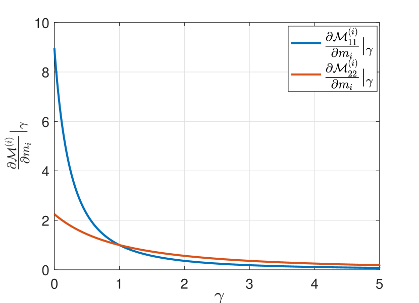
(a) First derivative of tensor components.

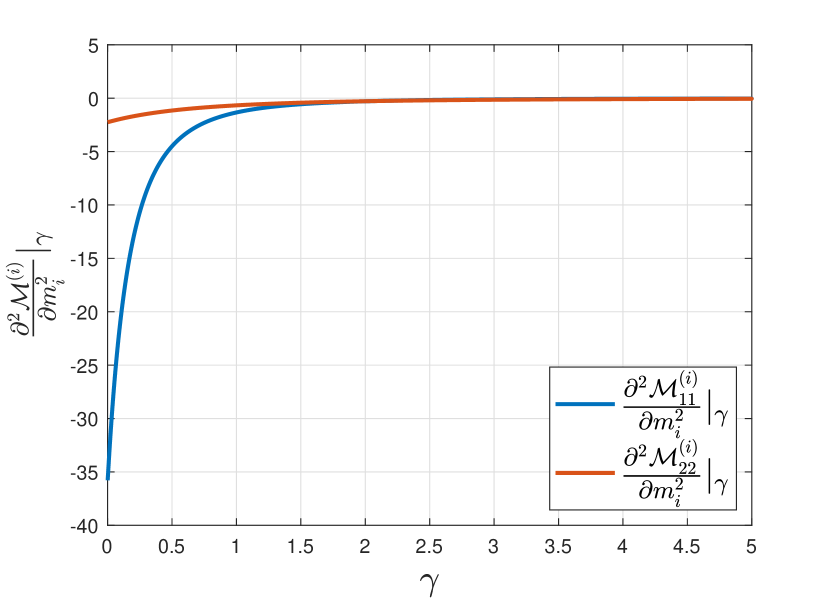
(b) Second derivative of tensor components.

Figure 2: Derivative of components of the polarization tensor for an ellipsoid $B$ with $a=1$, $b=2$, $|B|=1$.

The asymptotic approximations to derivatives (4.18) can be used to form a diagonal approximation $\tilde{\mathrm{H}}$ to the Hessian matrix,

$$\tilde{\mathrm{H}}_{ij}(\mathbf{m})=\left\{\begin{array}[]{ll}\sum_{r=1}^{N_{d}}\left\{\mathrm{C}_{ri}(\mathrm{m}_{i})^{2}+\mathrm{D}_{ri}(\mathrm{m}_{i})(\mathrm{f}_{r}-\mathrm{d}_{r})\right\}&\mbox{if }i=j\\ 0&\mbox{otherwise}.\end{array}\right.$$ (4.20)

From remark 4.1 above, this diagonal matrix will be a valid approximation for ${\mathbf{m}-\mathbf{m}_{0}}$ sufficiently sparse with sufficiently separated elements, where $\mathbf{m}_{0}$ is an initial homogeneous conductivity. Where this is not the case, those elements corresponding to nearby perturbations will neglect non-linear interactions between the elements, in which case the approximation (3.6) which this is based upon is no longer $\mathcal{O}(\epsilon^{d+1})$ accurate. (4.20) may still be a useful approximation, depending on how it is used, where these non-linear corrections are small – which is to be determined through numerical experimentation.

The components $\mathrm{C}_{ri}$ and $\mathrm{D}_{ri}$ are straightforward to calculate via (4.18) and (4.19), requiring only a small number of 2- or 3-d matrix-vector multiplications each. Moreover, the terms $\nabla u_{0}$ will already have been calculated during the calculation of the $u_{r}$, and, depending on the domain, an analytic expression for $\nabla_{z}N(x,z)$ may be available. This compares favourably to the full calculation (4.17), in which each element of the matrix requires another solution to the forward problem.

Equations (4.18) expresses the Fréchet derivative of the EIT forward problem as the derivatives of the asymptotic series. Similarly, Ammari et al[4, thm. 5.1] provide an expression for the first Fréchet derivative (4.11) of inhomogeneous GPTs with respect to an internal conductivity of the inclusion, which is given as the difference between two asymptotic series. This is used for a sensitivity analysis of GPTs to conductivity, to reconstruct inhomogeneous GPTs, and then subsequently reconstruct the inhomogeneous conductivity of an inclusion. The approach we present (and its application) is subtly different – for calculating derivatives, one could view our method as truncating the difference of these two series in [4, thm. 5.1] to first order, and identifying the difference between these remaining series in terms of Fréchet derivatives of polarization tensors themselves when taking the same limit. We then propose to reconstruct an inhomogeneous domain, rather than inhomogeneous inclusions.

Remark 4.2.

Note that in (4.18b) it is not possible to calculate mixed derivatives, due to the summation term in (3.6). We could consider mixed derivatives for closely-spaced inclusions, using the polarization tensor for two closely spaced inclusions. In other words, we might approximate the mixed derivative by

$$\frac{\partial^{2}\mathrm{f}_{r}}{\partial\mathrm{m}_{i}\partial\mathrm{m}_{j}}=-\epsilon_{(ij)}\nabla U(z_{(ij)})\frac{\partial^{2}\mathcal{M}^{(ij)}}{\partial{\mathrm{m}_{(ij)}}^{2}}\nabla_{z}N(x,z_{(ij)})+\mathcal{O}(\epsilon^{d+1}),$$ (4.21)

where $\mathcal{M}^{(ij)}$ is the polarization tensor of inclusion $B_{(ij)}=B_{i}\cup B_{j}$, for closely spaced (joining) elements $B_{i}$ and $B_{j}$, with weighted centre point $z_{(ij)}$, weighted average conductivity $\mathrm{m}_{(ij)}$, and size $\epsilon_{(ij)}$. In order for this to provide any computational benefit, one would need an easy way to determine (approximately) the equivalent ellipse/ellipsoid of two adjoining elements to write $\mathcal{M}^{(ij)}$ in the analytic form of the Pólya-Szegö tensor. Such composite object tensors have been calculated for example for the Eddy-current problem[6], but analytic expressions are not currently available.

4.3 Quasi-Newton inversion schemes

We consider solving the inverse problem (1.1) using a Newton-type method, which uses the update direction

$$\mathrm{B}^{[k]}\mathbf{p}^{[k]}=-\mathbf{g}^{[k]},$$ (4.22)

where $\mathbf{g}^{[k]}$ is the gradient for iterate $\mathbf{m}^{[k]}$ at iteration $k$, and $\mathrm{B}^{[k]}$ some approximation to the Hessian matrix. For a robust and efficient solution, we would expect an appropriate choice of $\mathrm{B}^{[k]}$ to have a similar structure to the true Hessian (i.e. having similar distribution of eigenvalues and eigenvectors), and require only a small number of solutions to the forward problem to calculate or update respectively. Additionally, it preferably has limited storage requirements, and the cost of solving (4.22) is not so large that it outweighs the reduction in number of forward problems solved.

We could use the diagonal approximate Hessian $\tilde{\mathrm{H}}^{[k]}$ from (4.20) directly in (4.22), denoting $\tilde{\mathrm{H}}^{[k]}:=\tilde{\mathrm{H}}(\mathbf{m}^{[k]})$. This would be computationally very cheap and ought to provide a good approximation to the spacing between contours of the objective function about the iterate $\mathbf{m}^{[k]}$, but it will not incorporate any information about the curvature of these contours. This could result in an update direction that deals reasonably well with different parameter illumination and the ill-posedness in certain directions, but less well with the non-linearity of the inverse problem.

We propose instead to use the approximate Hessian (4.20) as an initial Hessian approximation for a quasi-Newton method, updated each iteration, which is the main contribution of this paper. Some quasi-Newton methods such as l-BFGS allow a different initial Hessian approximation to be used at each iteration[45, pp. 177], which also allows us to update $\tilde{\mathrm{H}}^{[k]}$ for each iterate $\mathbf{m}^{[k]}$. We expect that such an approach should initialise the quasi-Newton method with good information about the ratio of eigenvalues at the current iterate (i.e. the spacing between contours of the objective function), allowing it to more effectively approximate the dominant eigenvectors within fewer iterations. This should far more rapidly build a good approximation to the true Hessian than, say, initialising with a multiple of the identity, providing information about the curvature of contours (non-linearity) which is not present in $\tilde{\mathrm{H}}^{[k]}$.

It is worth noting that for $\mathbf{m}^{[k]}$ containing perturbations not sufficiently separated, $\tilde{\mathrm{H}}^{[k]}$ may be a poor approximation to the diagonal of the Hessian. This may limit the effectiveness of our approach, but we could choose instead to initialise with $\tilde{\mathrm{H}}^{[0]}$ or otherwise some thresholded version.

4.3.1 Computational cost

Recall from Section 2.1 that $N_{E}$ denotes the number of elements in the reconstruction domain, $N_{N}$ the number of finite element nodes in the simulation domain, and $N_{L}-1$ the number of current vectors to generate the dataset of $N_{d}=\frac{1}{2}N_{L}(N_{L}-1)$ datapoints. Calculating $\tilde{\mathrm{H}}^{[k]}$ each iteration via (4.19), (4.18) and (4.20) involves $\mathcal{O}(N_{d}N_{E})$ operations as $N_{E},N_{L}\rightarrow\infty$. This ignores the one-time cost of calculating the Neumann functions in the first iteration which can then be stored in memory (or permanently for repeated experiments in the same domain). This is the same as the $\mathcal{O}(N_{d}N_{E})$ complexity to form the diagonal of the Gauss Newton approximate Hessian $\operatorname*{diag}(\mathrm{J}^{T}\mathrm{J})$, assuming $\mathrm{J}$ has already been formed and stored in calculation of the gradient of the objective function (otherwise this would be a $\mathcal{O}(N_{d}N_{N}^{3})$ complexity using an adjoint method).

Calculating the diagonal of the true Hessian via (4.17) has computational complexity $\mathcal{O}(N_{d}N_{E}N_{N}^{3})$, or $\mathcal{O}(N_{d}N_{E}^{2}N_{N}^{3})$ for the full (dense) matrix, with this high cost being driven by the need to re-simulate fields. These complexities provide an upper bound, reducing for a sparse Hessian matrix or if an LU decomposition of the system matrix $S$ has been calculated and stored. The computational complexity of the true Hessian is also reduced to $\mathcal{O}(N_{L}N_{E}N_{N}^{3})$ when calculated via an adjoint field approach, which also has a higher memory requirement of $\mathcal{O}(N_{L}N_{N}N_{E})$. These differing complexities and memory requirements for calculating the Hessian highlight the common trade-off between speed and memory use for iterative PDE-based reconstruction methods. Nonetheless, it will be significantly more expensive to calculate than the proposed approximate Hessian using either method, which has no requirement to re-calculate fields.

5 Numerical experimentation

In this section, we undertake some numerical experiments into the effectiveness of the approximate Hessian to initialise l-BFGS. We consider both the accuracy of this approximate Hessian, as well as how well the reconstruction scheme performs. We aim to show that this provides a computationally cheap way of incorporating second derivative information into reconstruction schemes, which in some cases helps to improves contrast of images, as well as improving the rate of convergence compared to methods which use only first-derivative information. Importantly, this method remains a feasible choice for large-scale problems in which either storing dense Hessian approximations or calculating second derivatives directly is prohibitively expensive, noting the discussion on computational cost in Section 4.3.1.

Our numerical experiments were implemented in Matlab using the developers version of the open-source EIT package EIDORS[46, 47], which uses the complete electrode model outlined in Section 2.1. Polarization tensor Hessian reconstructions were benchmarked against a fairly standard non-linear Gauss-Newton method to solve the optimisation problem in EIT as implemented by the EIDORS library function inv_solve_core. The functions and scripts used in this paper can also be obtained via the EIDORS developers SVN repository. This includes the polarization tensor Hessian approximation, the Neumann functions for a disc and free-space in 2D, as well as the inversion scheme. It also includes the calculation of the true Hessian via an adjoint method. Experiments were carried out on a 2D disc with radius $r_{0}=1$ with $N_{L}=16$ electrodes, of background conductivity $\sigma_{0}=1$. The meshes were created using the EIDORS function ng_mk_cyl_models, which calls routines from Netgen Mesher[48].

5.1 Validating the Hessian approximation

Qualitative comparison

We begin by comparing components of the approximate Hessian terms given by equations (4.18), (4.19) and (4.20) to the true Hessian components (4.4). For this, we take $\Omega$ to be the 2D unit disc. As discussed in Section 4.2, for simplicity we use the Steiner inellipse as the closest fitting ellipse to the triangular finite elements. For comparison, we also calculate approximate Hessian matrices in which we use the free-space Green’s function in place of the Neumann function – i.e. using the equivalent expression to (3.2) for free-space. This helps to illustrate the extent to which boundary interactions are included in the model.

Figure 3 shows the diagonal of the true and approximate Hessian matrices, calculated in a homogeneous reconstruction domain, in which data was simulated for a domain with a single circular inclusion with conductivity $\sigma=2.3\sigma_{0}$, radius $0.25$, centred at $(0.3,0.3)^{T}$. These simulations were repeated for different inclusion conductivities $0.5\sigma_{0}<\sigma<5\sigma_{0}$, and selected elements $H_{ii}$ (away from the boundary) are shown as a function of inclusion conductivity $\sigma$ in Figure 4. We see that away from the domain boundary (and in particular away from the electrodes) the Polarization Tensor Hessian is qualitatively similar, and when using the Neumann function for a disc we have a reasonable approximation. As the conductivity of the inclusion $\sigma$ in the simulation domain is varied, the Hessian approximation calculated for a homogeneous domain simply vary linearly with the data residual $\delta\mathbf{d}$ (which itself varies non-linearly with $\sigma$); this appears sufficient to capture the main non-linear features.

Closer to the boundary the approximation appears poor. The indexing of elements is such that all of those from 197 to 256 share at least a node with an electrode in the FEM mesh (and so also touch the boundary), and every element from 225 has an edge on the boundary (with every other of these being an electrode). Given this numbering, from Figure 3 it would appear that in this case you do not need to move far from the boundary (or electrodes) before a reasonable approximation is gained. In all cases, using the free-space Green’s function (red lines in Figures 3 and 4) in place of the Neumann function, and thus neglecting any effects of boundary interaction, results in a much poorer approximation apart from in the centre of the domain.

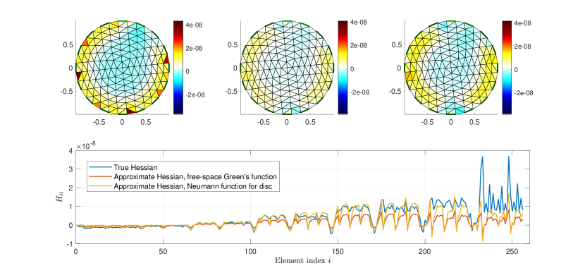
Figure 3: Comparison of true and approximate diagonals of the Hessian matrix calculated on a homogeneous disc, for simulated data with a single inclusion with conductivity $\sigma=2.3$. The true Hessian is shown top-left (with elements of the matrix mapped to their corresponding element in the domain) and in blue below. The approximate Hessian using the freespace Green’s function is shown top-centre and in red below. The approximate Hessian using the Neumann function for the disc is shown top-right, and in yellow below. Higher element indices correspond to elements closer to the boundary.

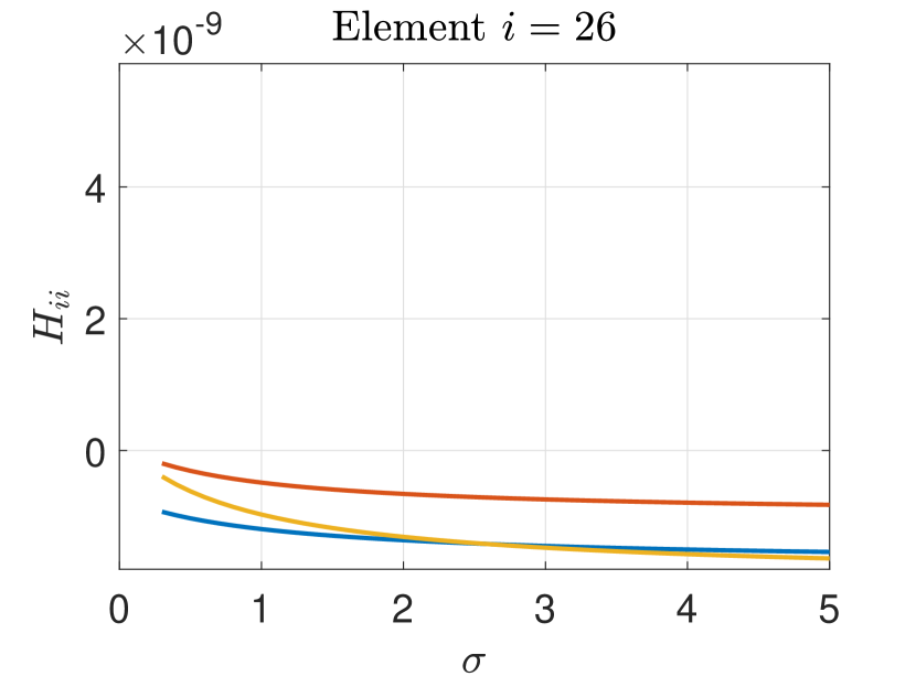
(a) Element 26, between the inclusion and domain centre.

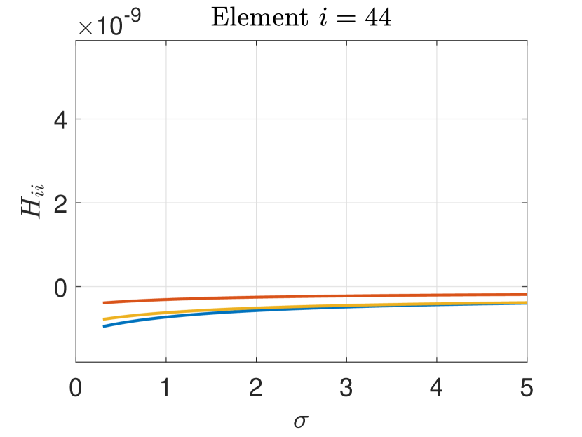
(b) Element 44, within the inclusion.

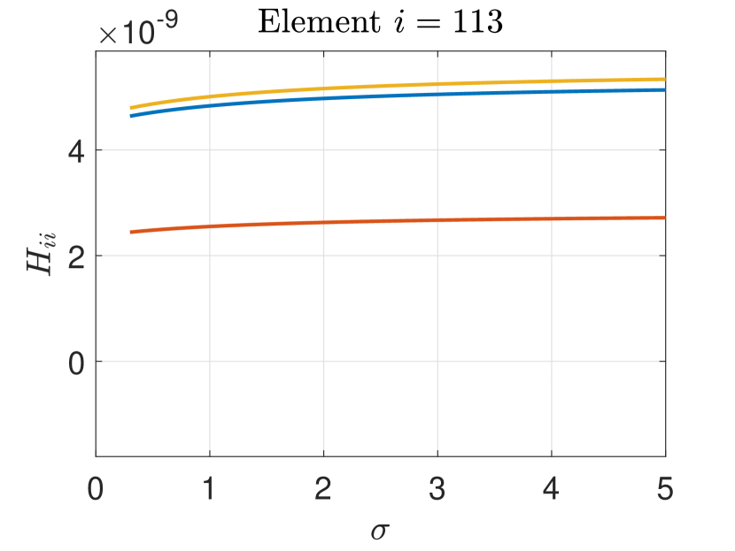
(c) Element 113, between the inclusion and the boundary.

Figure 4: $H_{ii}$ for selected elements $i$ away from the boundary, as a function of inclusion conductivity $\sigma$. Blue shows the true Hessian, and red and yellow the approximations using the free space Green’s function and Neumann function on a unit disc, respectively.

Principal angles and quantitative comparison

To help understand the utility as well as accuracy of the approximate Hessian $\tilde{\mathrm{H}}$ initialised BFGS matrix, we look at both the relative residual between the true and BFGS Hessian in the Frobenius norm, as well as how their (dominant) singular vectors are aligned with the true matrices. The latter will suggest how closely the l-BFGS approximate Hessians will act on a gradient vector to change the update direction, closer to that of the true Hessian if the singular vectors are more closely aligned, but ignores possible scaling differences (which are easily resolved through a linesearch or within the quasi-Newton update itself). To compare singular vectors, we use the principal angles $\Theta$ between the subspaces they span via[49]

$$\cos\Theta=\Sigma(\mathrm{V}^{H}\mathrm{W}),$$ (5.1)

where $\Sigma(\mathrm{A})$ denotes the singular values of $\mathrm{A}$, and $\mathrm{V}$, $\mathrm{W}$ are the matrices whose columns are the right singular vectors.

We compare the right singular vectors associated with the 20 largest singular values. Comparing a large number of singular vectors results in subspaces which are almost the same (since each complete set form an orthonormal basis, taking all of them would give the same subspace), whereas a small number provides little to compare and so subspaces will generally be orthogonal. Other choices of a similar magnitude would be equally valid.

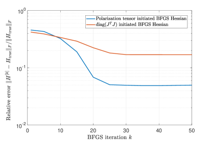
Figure 5: Relative error of the BFGS approximate Hessian to the true Hessian in Frobenius norm, initialised by the polarization tensor approximation (blue) and $\operatorname*{diag}(\mathrm{J}^{T}\mathrm{J})$ (red).

Figure 5 shows the relative error in Frobenius norm of the BFGS to true Hessian matrix against BFGS iteration. The BFGS matrix initialised by $\tilde{\mathrm{H}}$ is shown in blue, and by $\operatorname*{diag}(\mathrm{J}^{T}\mathrm{J})$ in red, for up to 50 BFGS iterations. The $\tilde{\mathrm{H}}$ initialisation clearly enables a much better approximation, reaching approximately 4% relative error after 25 iterations versus greater than 10% for the $\operatorname*{diag}(\mathrm{J}^{T}\mathrm{J})$ initialisation. In this scenario, both BFGS initialisations make very little further improvement after 25 iterations. This is likely due to update directions $\mathbf{p}^{[k]}$ being similar across later iterations, as well as progressively smaller in norm, as the $\mathbf{x}^{[k]}$ converge to the solution, so little additional information about the Hessian (or its action on differing vectors) is gained.

Figure 6 shows the principal angles between the subspace spanned by the first 20 singular vectors of the true and BFGS approximate Hessians after a number of outer BFGS iterations. In Figure 6a, the Hessian was initialised with $\tilde{\mathrm{H}}$, and in Figure 6b it was initialised with $\operatorname*{diag}(\mathrm{J}^{T}\mathrm{J})$. It is clear from these that the $\tilde{\mathrm{H}}$ initialisation is also much better able to resolve the dominant eigendirections of the Hessian. For example, after 5 iterations the $\tilde{\mathrm{H}}$ Hessian has 10 principal angles less than $\pi/15\approx 0.21$, but the $\operatorname*{diag}(\mathrm{J}^{T}\mathrm{J})$ initialisation still has only 7 similarly small angles after a full 50 iterations.

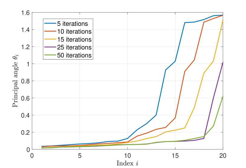
(a) $\tilde{\mathrm{H}}$ initiated BFGS Hessian.

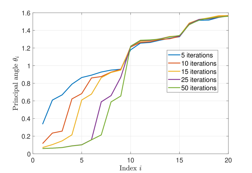
(b) $\operatorname*{diag}(\mathrm{J}^{T}\mathrm{J})$ initiated BFGS Hessian.

Figure 6: Principal angles $\theta_{i}$ between subspaces $\mbox{span}(\tilde{\mathrm{V}})$ and $\mbox{span}(\tilde{\mathrm{W}})$, where $\tilde{\mathrm{V}}$ and $\tilde{\mathrm{W}}$ are the matrices formed by the first 20 right singular vectors of the true Hessian $\mathrm{H}$ and BFGS approximate Hessian $\mathrm{B}^{[k]}$, respectively, after $k$ BFGS iterations. In Figure 6a the BFGS approximate Hessian is initialised with the diagonal polarization tensor Hessian approximation, and in 6b it is initiated with $\operatorname*{diag}(\mathrm{J}^{T}\mathrm{J})$.

5.2 Reconstruction results

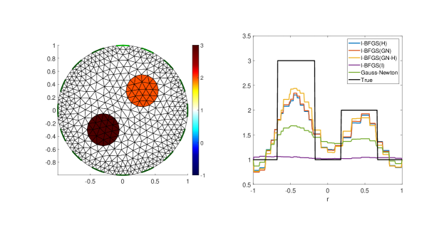
(a) True domain (left), and slice through $x=y$ of reconstructions (right).

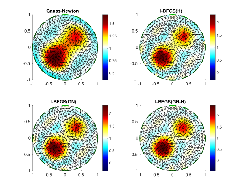
(b) Reconstruction results with Gauss-Newton and l-BFGS

Figure 11: Final reconstruction results after the numerical stagnation condition (5.3) was met for a unit circular domain containing two inclusions of radius 0.25$r_{0}$, separation 0.3$r_{0}$.

The approximate diagonal Hessian is now used as the initial Hessian in an l-BFGS reconstruction scheme. Four data sets are simulated for unit circle domains containing two circular inclusions with $\sigma=2\sigma_{0}$ and $\sigma=3\sigma_{0}$, respectively. For each, independent and identically distributed Gaussian noise is added with a signal-to-noise ratio of 50. Figures 8, 9 and 10 show the true domain and reconstruction results for inclusions of radius $0.16r_{0}$, separated from the origin by $0.25r_{0},0.3r_{0}$ and $0.4r_{0}$, respectively. Figure 11 shows the true domain and reconstruction results for inclusions of radius $0.25r_{0}$, separated from the origin by $0.3r_{0}$. In each case, the reconstruction domain has $N_{m}=N_{E}=800$ elements.

Homogeneous backgrounds are used for easier assessment of reconstruction results versus objects size and distance apart, rather than the objects varying contrast to the background. However, our previous work for GPR imaging demonstrates the method can equally be applied to reconstruction problems with an unknown inhomogeneous background[24].

Four reconstructions are presented for each simulated data set, resulting from different reconstruction algorithms. These are:

• Gauss-Newton;

• l-BFGS with initial Hessian approximation given by

  • Polarization tensor approximate Hessian $\tilde{\mathrm{H}}$, referred to as l-BFGS(H),

  • $\operatorname*{diag}{(\mathrm{J}^{T}\mathrm{J})}$, referred to as l-BFGS(GN),

  • $\operatorname*{diag}{(\mathrm{J}^{T}\mathrm{J})}$ plus the second derivative part of the polarization tensor approximate Hessian, referred to as l-BFGS(GN-H).

The regularisation term for each was

$$R(\mathbf{m})=\|\mathrm{L}\mathbf{m}\|_{2}^{2},$$ (5.2)

with $\mathrm{L}$ the discrete Laplace operator in 2D, and a regularisation parameter of $\lambda=5\times 10^{-5}$ (chosen heuristically to provide the best stable Gauss-Newton results as a benchmark). The regularisation term was also included in the initial Hessian approximation for each of the l-BFGS methods. Each reconstruction was stopped when the relative change in residual met the numerical stagnation condition

$$\frac{\mathcal{J}(\mathbf{m}^{[k-1]})-\mathcal{J}(\mathbf{m}^{[k]})}{\mathcal{J}(\mathbf{m}^{[0]})}<10^{-4},$$ (5.3)

which is the default condition of the EIDORS Gauss-Newton solver.

From figures 8 through 10, we see that the variants of l-BFGS are generally better able to separate the two inclusions than Gauss-Newton, which tends to result in reconstructions with the two inclusions blurred together more. The results of l-BFGS(H) and l-BFGS(GN) are almost indistinguishable, providing acceptable separation and sizing of the inclusions as well as showing some contrast between the two. This is a favourable result, as l-BFGS(H) may be slightly less computationally expensive if the Jacobian matrix is not being calculated and stored (e.g. if an adjoint method is being used to calculate gradients).

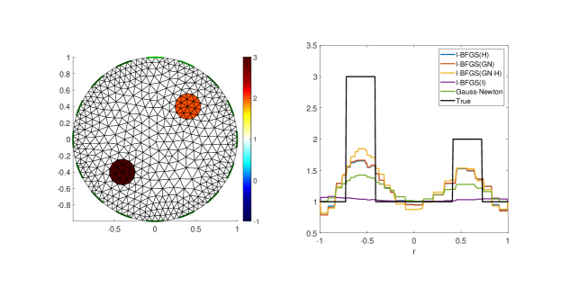
(a) True domain (left), and slice through $x=y$ of reconstructions (right).

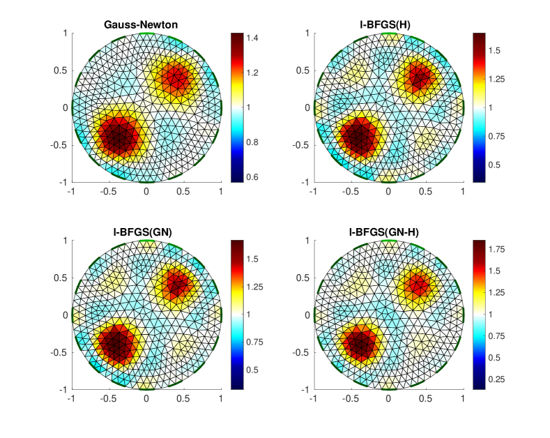
(b) Reconstruction results with Gauss-Newton and l-BFGS

Figure 10: Final reconstruction results after the numerical stagnation condition (5.3) was met for a unit circular domain containing two inclusions of radius 0.16$r_{0}$, separation 0.4$r_{0}$.

In Figures 10 and 11, l-BFGS(GN-H) also results in a slightly better contrast estimation of the two inclusions, but otherwise similar (or indistinguishable) results. Since this is also a computationally inexpensive addition to calculating the Gauss-Newton diagonal, we would also suggest this is a favourable result.

Since the visual quality of reconstruction results alone is not a sufficient measure of utility, the relative residual of the objective function against l-BFGS iteration is given in Figure 7. We see that l-BFGS(H) has a slightly slower rate of convergence than l-BFGS(GN), though the difference is generally marginal, and l-BFGS(GN-H) generally outperforms both. Indeed, for the three reconstruction problems with inclusions further from the boundary, l-BFGS(GN-H) converges in approximately 30 iterations fewer than the other two methods. These results are displayed against l-BFGS iteration, and it may be interesting also to directly compare e.g. CPU time. However, since EIDORS uses efficient factorisation and caching methods to form the Jacobian during the solution to the forward problem it would be impractical to develop our proposed method to a similar standard for a useful comparison. Moreover, considering the additional cost of forming $\tilde{\mathrm{H}}$ is similar to that of $\mathrm{J}^{T}\mathrm{J}$ (see Section 4.3), we would expect little difference to the appearance of these results.

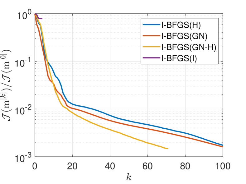
(a) Inclusion radius $0.16r_{0}$, separation 0.25$r_{0}$

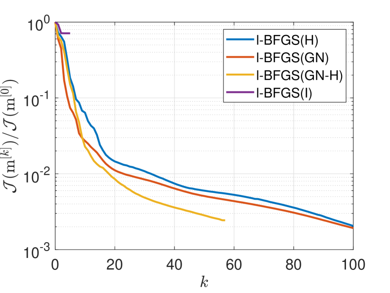
(b) Inclusion radius 0.16$r_{0}$, separation 0.3$r_{0}$

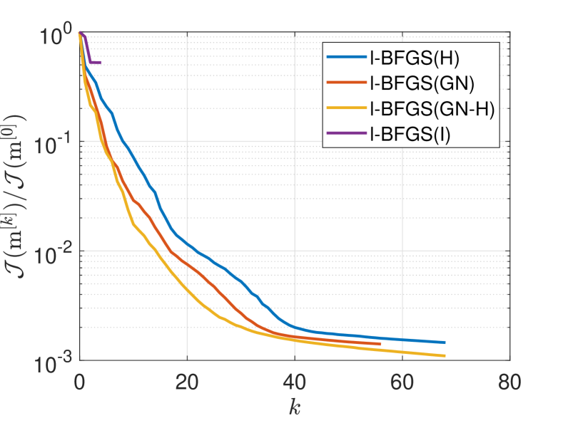
(c) Inclusion radius 0.16$r_{0}$, separation 0.4$r_{0}$

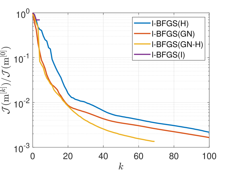
(d) Inclusion radius 0.25$r_{0}$, separation 0.3$r_{0}$

Figure 7: Objective function relative residual $\mathcal{J}(\mathbf{m}^{[k]})/\mathcal{J}(\mathbf{m}^{[0]})$ against l-BFGS iteration $k$ for the four reconstruction problems.

These results are not unexpected: l-BFGS(GN-H) provides the small second derivative correction to the exact Gauss-Newton diagonal, resulting in a more accurate approximation to the true Hessian and with that faster convergence. With inclusions close to the boundary though, the polarization tensor approximation is known to break down, and the performance improvement is negligible (though it still continues to progress a few iterations beyond the other methods for a slightly improved solution). For l-BFGS(H), it would appear that this second derivative correction has less impact than the inaccuracy of the first derivative approximation, hence performance is not improved over l-BFGS(GN).

We also attempted to use l-BFGS initiated with the identity (denoted l-BFGS(I) in Figure 7), but in each case it stagnated before any reasonable progress was made. This is seen in the slices through reconstructions in figures 8 through 10 (purple line) as well as the convergence results in Figure 7. So, at the very least, l-BFGS(H) provides a computationally viable quasi-Newton method where memory constraints are a concern. Then, l-BFGS(GN-H) provides a particularly computationally cheap and effective way to incorporate second derivative information as compared to calculating these terms directly.

6 Conclusion

Our motivation in this work has been to effectively deal with non-linearity in inverse boundary value problems for PDEs. This includes both a lack of superposition of data caused by multiple nearby inclusions, as well as the saturation effect as the material contrast of a single inclusion increases. In many problems involving well-isolated inclusions, solutions to the forward problem exist in the form of asymptotic expansions with polarization tensors. These can be used to find efficient and robust solutions to the inverse problem. However, they become invalid where there are nearby inclusions and the lack of superposition becomes a more dominant effect. In such cases, one often poses the inverse problem as a least-squares one, for which the Hessian matrix is known to be important in finding efficient and robust solutions.

Our contribution has been to use the polarization tensors to derive a computationally cheap approximate diagonal Hessian matrix, which describes the saturation effect and ill-posedness due to parameter illumination. We have proposed to use this either as an initial Hessian approximation in quasi-Newton schemes, or to provide the second derivative correction in addition to $\operatorname*{diag}(\mathrm{J}^{T}\mathrm{J})$ for such methods. Through our numerical experimentation with the EIT problem, we have shown that in the first case this provides a computationally viable quasi-Newton method for non-linear inverse problems which may have memory constraints. In the latter case, where one is able to calculate the Jacobian matrix itself, this provides a particularly inexpensive way to incorporate second derivative information which in some cases may have a significant positive impact on performance. Our numerical experimentation consisted of not just the reconstruction problems with simulated data, but also looked at the accuracy of derivative approximations themselves. We present this as a proof-of-principle for this mixed-model approach to solving non-linear inverse problems, potentially usable for any imaging modality in which a polarization tensor approximation to the forward model exists.

We have suggested some further work throughout this paper. Firstly, our choice of “closest fitting ellipse” to the triangular elements (in the electrical sense of (3.4)) as the Steiner inellipse is taken for computational simplicity. The development of either explicit results or a more precise heuristic rule might be used to improve this method. Secondly, as only a proof-of-principle has been presented, the methods should be tested on realistic large 3D problems in which memory is a constraint, including other imaging modalities besides EIT.

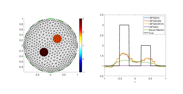
(a) True domain (left), and slice through $x=y$ of reconstructions (right).

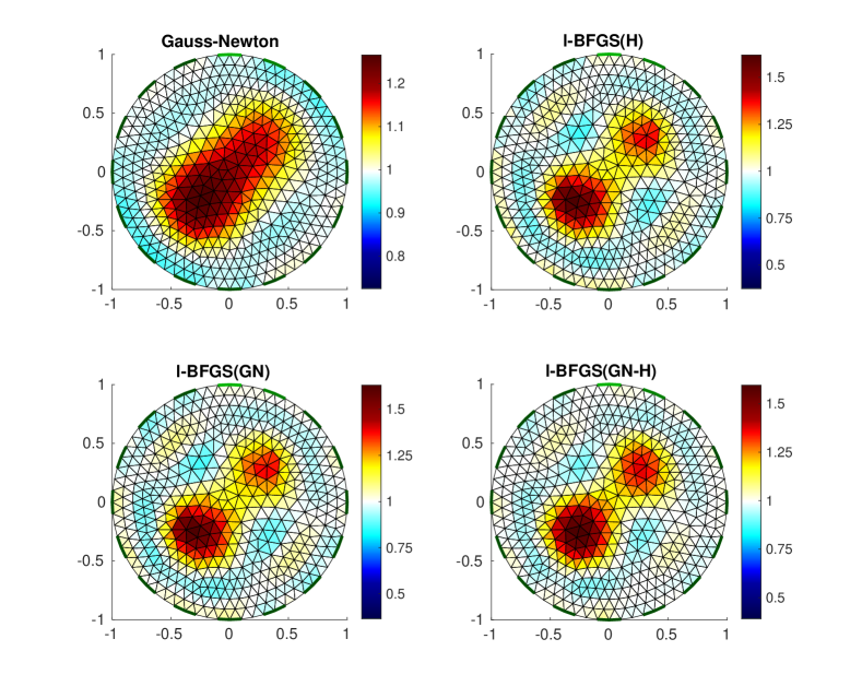
(b) Reconstruction results with Gauss-Newton and l-BFGS

Figure 8: Final reconstruction results after the numerical stagnation condition (5.3) was met for a unit circular domain containing two inclusions of radius 0.16$r_{0}$, separation 0.25$r_{0}$.

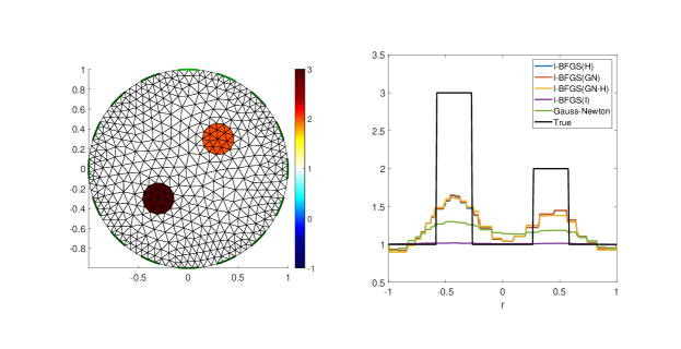
(a) True domain (left), and slice through $x=y$ of reconstructions (right).

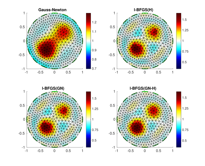
(b) Reconstruction results with Gauss-Newton and l-BFGS

Figure 9: Final reconstruction results after the numerical stagnation condition (5.3) was met for a unit circular domain containing two inclusions of radius 0.16$r_{0}$, separation 0.3$r_{0}$.

References

- [1]
- [2] Ammari H, Kang H, Lim M. Polarization tensors and their applications. Journal of Physics: Conference Series. 2005;12(1):13.
- [3] Ledger PD, Lionheart WRB. Characterizing the shape and material properties of hidden targets from magnetic induction data. IMA Journal of Applied Mathematics. 2015;80(6):1776–1798.
- [4] Ammari H, Deng Y, Kang H, et al. Reconstruction of inhomogeneous conductivities via the concept of generalized polarization tensors. In: Annales de l’Institut Henri Poincare (C) Non Linear Analysis; Vol. 31; Elsevier; 2014. p. 877–897.
- [5] Lionheart WRB, Khairuddin TKA. Polarization tensors and object recognition in weakly electric fish. In: Biologically-inspired radar and sonar: Lessons from nature. Institution of Engineering and Technology; 2017. Radar, Sonar & Navigation; p. 229–250.
- [6] Ledger PD, Lionheart WRB, Amad AAS. Characterisation of multiple conducting permeable objects in metal detection by polarizability tensors. Mathematical Methods in the Applied Sciences. 2019;42(3):830–860.
- [7] Ammari H, Iakovleva E, Lesselier D, et al. MUSIC-type electromagnetic imaging of a collection of small three-dimensional bounded inclusions. SIAM Journal on Scientific Computing. 2007;29(2):674–709.
- [8] Kleinman R, Senior T. Rayleigh scattering. In: Varadan V, Varadan V, editors. Low and high frequency asymptotics. North-Holland; 1986. p. 1–70.
- [9] Tarantola A, Valette B. Generalized nonlinear inverse problems solved using the least squares criterion. Reviews of Geophysics. 1982;20(2):219–232.
- [10] Vogel CR. Computational methods for inverse problems. Society for Industrial and Applied Mathematics; 2002.
- [11] Martínez JLF, niz MZFM, Tompkins MJ. On the cost functional in linear and nonlinear inverse problems. Geophysics. 2012;77(1):W1–W15.
- [12] Pratt RG, Shin C, Hicks G. Gauss-Newton and full Newton methods in frequency-space seismic waveform inversion. Geophysical Journal International. 1998;133(2):341–262.
- [13] Haber E, Ascher UM, Oldenburg D. On optimization techniques for solving nonlinear inverse problems. Inverse Problems. 2000;16(5):1263.
- [14] Bui-Thanh T, Ghattas O. Analysis of the Hessian for inverse scattering problems: I. inverse shape scattering of acoustic waves. Inverse Problems. 2012;28(5):055001.
- [15] Bui-Thanh T, Ghattas O. Analysis of the Hessian for inverse scattering problems: II. inverse medium scattering of acoustic waves. Inverse Problems. 2012;28(5):055002.
- [16] Bui-Thanh T, Ghattas O. Analysis of the Hessian for inverse scattering problems: III. inverse medium scattering of electromagnetic waves in three dimensions. Inverse Problems and Imaging. 2013;7(4):1139–1155.
- [17] Schweiger M, Arridge SR, Nissilä I. Gauss-Newton method for image reconstruction in diffuse optical tomography. Physics in Medicine & Biology. 2005;50(10):2365–86.
- [18] Kaltenbacher B, Hofmann B. Convergence rates for the iteratively regularized Gauss-Newton method in Banach spaces. Inverse Problems. 2010;26(3):035007.
- [19] Haber E. Quasi-newton methods for large-scale electromagnetic inverse problems. Inverse Problems. 2005;21(1).
- [20] Lavoué F, Brossier R, Métivier L, et al. Two-dimensional permittivity and conductivity imaging by full-waveform inversion of multioffset GPR data: a frequency-domain quasi-Newton approach; 2014. Pre-print accepted to Geophysics Journal International.
- [21] Santosa F, Symes WW. Computation of the Hessian for least-squares solutions of inverse problems of reflection seismology. Inverse Problems. 1987;4(1):211–233.
- [22] Jin Q. Inexact Newton-landweber iteration for solving nonlinear inverse problems in banach spaces. Inverse Problems. 2012;28(6):065002.
- [23] Métivier L, Brossier R, Virieux J, et al. Full waveform inversion and the truncated Newton method. SIAM Journal on Scientific Computing. 2013;35(2):B401–B437.
- [24] Watson FM. Better imaging for landmine detection: an exploration of 3D full-wave inversion for ground-penetrating radar. Doctor of philosophy. School of Mathematics, Faculty of Engineering and Physical Sciences, University of Manchester; 2015.
- [25] Watson F. Towards 3D full-wave inversion for GPR. In: 2016 IEEE Radar Conference (RadarConf); May; 2016. p. 1–6.
- [26] Lionheart WRB, Polydorides N, Borsic A. The Reconstruction Problem. In: Holder D, editor. Electrical Impedance Tomography: Methods, History and Applications. Institute of Physics; 2005.
- [27] Borcea L. Electrical impedance tomography. Inverse Problems. 2002;18:R99–R136.
- [28] Uhlmann G. Electrical impedance tomography and Calderón’s problem. Inverse Problems. 2002;25(12):123011.
- [29] Somersalo E, Cheney M, Isaacson D. Existence and uniqueness for electrode models for electric current computed tomography. SIAM Journal on Applied Mathematics. 1992;52(4):1023–1040.
- [30] Elman HC, Silvester DJ, Wathen AJ. Finite Elements and Fast Iterative Solvers: With Applications in Incompressible Fluid Dynamics. 2nd ed. Oxford University Press; 2006.
- [31] Ciarlet PG. The Finite Element Method for Elliptic Problems. 1st ed. North-Holland; 1978.
- [32] Zienkiewicz OC. The Finite Element Method. 3rd ed. McGraw-Hill; 1977.
- [33] Vauhkonen M. Electrical Impedance Tomography and Prior Information Doctor of philosophy. University of Kuopio, Finland; 1997.
- [34] Ledger PD. hp-Finite element discretisation of the electrical impedance tomography problem. Computer Methods in Applied Mechanics and Engineering. 2012;225-228:154–176.
- [35] Crabb MG. Convergence study of 2D forward problem of electrical impedance tomography with high-order finite elements. Inverse Problems in Science and Engineering. 2017;25(10):1397–1422.
- [36] Ammari H, Kang H. Polarization and moment tensors, with applications to inverse problems and effective medium theory. Springer-Verlag, New York; 2007.
- [37] Cedio-Fengya DJ, Moskow S, Vogelius MS. Identification of conductivity imperfections of small diameter by boundary measurements. continuous dependence and computational reconstruction. Inverse Problems. 1998;14:553–595.
- [38] Ammari H, Kang H. Generalized polarization tensors, inverse conductivity problems, and dilute composite materials: A review. In: Contemporary mathematics. Vol. 408. American Mathematical Society; 2006. p. 1–68.
- [39] Khairuddin TKA, Lionheart WRB. Fitting ellipsoids to objects by the first order polarization tensor. Malaya Journal of Matematik. 2013;4:44–53.
- [40] Plessix RE. A review of the adjoint-state method for computing the gradient of a functional with geophysical applications. Geophysical Journal International. 2006;167(2):495–503.
- [41] Dobson DC. Convergence of a Reconstruction Method for the Inverse Conductivity Problem. SIAM Journal on Applied Mathematics. 1992;52(2):442–458.
- [42] Arridge S, Moskow S, Schotland JC. Inverse Born series for the Calderon problem. Inverse Problems. 2012;28(3):035003.
- [43] Weisstein EW. “Steiner Inellipse”. From MathWorld – a Wolfram Web Resource. [https://mathworld.wolfram.com/SteinerInellipse.html]; accessed 09/04/2020.
- [44] Marden M. Geometry of polynomials. Second edition ed. American Mathematical Society, Providence, Rhode Island; 1966.
- [45] Nocedal J, Wright SJ. Numerical Optimization. 2nd ed. Springer; 2000.
- [46] Adler A, Lionheart WRB. Uses and abuses of EIDORS: an extensible software base for EIT. Physiological Measurement. 2006;27:S25–S42.
- [47] Adler A, Boyle A, Braun F, et al. EIDORS Version 3.9. In: Proceedings International Conference on Biomedical Applications of EIT; 2017. p. 63.
- [48] Schöberl J. NETGEN An advancing front 2D/3D-mesh generator based on abstract rules. Computing and Visualization in Science. 1997;1:41–52.
- [49] Golub GH, Loan CFV. Matrix computations. 4th ed. John Hopkins University Press; 2013.