Filtering Empty Camera Trap Images in Embedded Systems

Abstract

Monitoring wildlife through camera traps produces a massive amount of images, whose a significant portion does not contain animals, being later discarded. Embedding deep learning models to identify animals and filter these images directly in those devices brings advantages such as savings in the storage and transmission of data, usually resource-constrained in this type of equipment. In this work, we present a comparative study on animal recognition models to analyze the trade-off between precision and inference latency on edge devices. To accomplish this objective, we investigate classifiers and object detectors of various input resolutions and optimize them using quantization and reducing the number of model filters. The confidence threshold of each model was adjusted to obtain 96% recall for the nonempty class, since instances from the empty class are expected to be discarded. The experiments show that, when using the same set of images for training, detectors achieve superior performance, eliminating at least 10% more empty images than classifiers with comparable latencies. Considering the high cost of generating labels for the detection problem, when there is a massive number of images labeled for classification (about one million instances, ten times more than those available for detection), classifiers are able to reach results comparable to detectors but with half latency. 

1 Introduction

The use of camera traps is a strategy for passive wildlife monitoring that involves installing cameras with presence sensors that, when triggered, activate a process of recording short sequences of images or videos of animals. The objective aimed on this strategy is to generate data showing animal in their daily lives, without interfering with the animals’ natural behavior [13]. However, it is very common to have a very large number of images collected with no animals (empty) due to sensor accidental triggering, e.g. about 75% of the images from the Snapshot Serengeti dataset do not contain animals [18].

In recent years, several studies have investigated the use of deep learning models to recognize animals in camera trap images [2, 13, 17, 19, 24, 25]. Due to the development of new technologies for this type of monitoring, embedding models to identify animals directly in the devices may provide advantages. For instance, in projects whose equipment is connected to a network, prior filtering avoids the unnecessary transmission of empty images, saving network bandwidth and energy [4]. Another example are traditional approaches, which usually involve going to the capture points to retrieve cameras and/or memory cards [22]. In this case, discarding empty images can save data storage, extending the time a camera can stay in the field collecting images without needing maintenance.

Although there are studies comparing the performance of several modern deep learning architectures on recognizing animals in camera trap images [13, 17, 24], there are few studies regarding the trade-off between model performance and inference latency directly on edge devices. In [23], Tydén and Olsson evaluate object detection models on a Raspberry Pi applied to recognize animals. However, the used image dataset is composed of 4,000 instances comprising only 8 species, limiting the scope of the conclusions. In a similar strategy, Zualkernan et al. [27] evaluate several classifiers on a Raspberry Pi aiming to identify animals. Nonetheless, they do not detail latency assessment. Finally, Schneider et al. [17] suggest that detection models would be better than classification models for recognizing animals, but requiring higher computational power on the other hand. Thus, this work presents a comparative study between classifiers and detectors of different complexities running on edge devices to recognize nonempty images.

Our main findings are as follows:

• Detection models generally outperform classifiers with comparable latency if they are trained on the same camera trap image set.

• Classifiers can obtain high performance on empty image identification, given the difficulty of generating labels to train detectors. The performance, however, depends on the amount of images available for training, as well as on specific factors that can vary from dataset to dataset.

• Models with a higher input resolution perform better. Their inference latency can be kept low by reducing the number of model filters at an acceptable performance cost for the problem.

2 Related Work

Several works apply deep learning techniques to recognise animals in camera trap images. Some studies classify the species assuming that an animal has already been identified on the scene [24]. A second approach adds an extra class to the model to identify empty images, sometimes called negative class or background class [2, 17, 19]. There are also approaches composed of two stages. In the first stage, a model recognizes whether there are animals in the scene, while in the second stage another model is responsible for the species identification [13, 25].

From a different perspective, animal detection-based approaches first focus on localizing animals in images and further classifying their species. In this context, MegaDetector [1] is a model based on the Faster R-CNN [14] object detector trained on a large number of camera trap images whose objective is to be a generalist animal detector. MegaDetector was trained to be capable of localizing animals in images from different ecosystems in the world, even species not seen during its training. Its primary idea is not species identification but only to find and localize animals. The species identification task must be performed by a classifier trained specifically for each project. However, since not all images used for training MegaDetector are publicly available due to licensing restrictions, it is not possible to reproduce the same experimental conditions as in [1]. In addition, Faster R-CNN requires high processing power and is not suitable for running on edge devices [16].

In line with the idea of reducing complexity, some studies compare the accuracy of Convolutional Neural Networks of varied complexities in the task of extracting information from camera trap images using classification models [13, 17, 23, 24]. Norouzzadeh et al. [13] trained several architectures to recognize nonempty images. In their experiments, the VGG16 architecture reached the best result, precisely 96.8% of accuracy rate. It is noteworthy, however, that ResNet18 achieved an accuracy of 96.3%, just 0.5% below the accuracy attained by VGG16, and equal to or higher than other deeper models in the same ResNet family. On the other hand, even though ResNet18 is less complex, it was not designed for inference on edge devices.

The scenario is different in [17], where Schneider et al.evaluated more efficient and lightweight deep models, including the MobileNetV2 and NASNetMobile architectures, in animal species classification. These models, designed specifically for computationally limited devices, reached accuracy 2.5% and 5% (in absolute values) lower than accuracy attained by DenseNet201 - the high-complex baseline. As expected, DenseNet201 achieved the best result: accuracy of 95.6% when tested on images from the same training locations; and 68.7% on images from locations not trained on.

Despite investigating more efficient and/or lightweight deep models, previously mentioned works did not focus on carrying out tasks on computationally limited devices. This is precisely the objective aimed on Tydén and Olsson’s work [23]. These authors study the trade-off between computational performance and accuracy of the SSD [12] detector and its optimized version SSDLite [16] (using InceptionV2 and MobileNetV2 as backbones) to recognize animals using the Raspberry Pi development board. However, the dataset investigated is composed of approximately only 4,000 images distributed among 8 classes, which may impose a limitation to the scope of the conclusions provided.

Finally, in terms of classifiers, Zualkernan et al. [27] evaluate InceptionV3, DenseNet121, ResNet18 and MobileNetV2 models on animal recognition using a dataset composed of 34,000 images. Despite comparing all these models in terms of accuracy, only InceptionV3 was evaluated on a Raspberry Pi 4B to verify inference latency.

Therefore, in this work, several architectures developed specifically for low computational power devices are analyzed to perform the task of animal recognition in camera trap images. Instead of focusing on a specific set of species, we analyse in this work the models’ ability to recognize animals, regardless of their species, similar to the process proposed for MegaDetector [1]. In this case, we test images from the same training sites and from new locations, as it is also done in [17]. However, unlike the latter, which investigated only classification models, in this work we compare classification and detection models. In addition, we evaluate other optimization approaches, such as quantization and reducing the number of model filters.

3 Materials and Methods

Two datasets are investigated in this paper: 1) Caltech Camera Traps; and 2) Snapshot Serengeti (SS). These datasets are described below.

3.1 Datasets

Caltech Camera Traps [2]: It contains 243,100 images taken from 140 capture locations in the Southwestern United States. The instances were labeled in 22 categories, and about 66,000 bounding boxes localizing animals were also provided. For our experiments, we selected a subset of images from the empty and nonempty classes, grouping into the nonempty class images from all other categories that have bounding boxes. Then, the dataset was partitioned into training and validation set according to the locations recommended in [9]. Moreover, a subset of the training partition was split, consisting of 20 locations chosen at random, to be used to adjust the training hyper-parameters (called here validation dev). Due to the fact that some locations concentrate a large number of images of the empty class, which may lead the models to be biased in certain backgrounds, we decided to limit to 1000 instances per location the number of empty class instances in both training and validation dev partitions. Table 1 summarizes the number of instances obtained.

Class	Training	Val_dev	Validation
Empty	8574	2824	19892
Nonempty	32032	3877	23410

Table 1: Number of images used from the Caltech dataset. The empty class of training and validation dev partitions was limited to 1000 instances per location. The nonempty class is composed of images with bounding boxes from all other categories.

Snapshot Serengeti [18]: This dataset currently contains more than 7 million camera trap images collected over 11 seasons in the Serengeti National Park, Tanzania. In this work, we use images from the first six seasons in order to keep consistency with previous works using the Snapshot Serengeti dataset [13, 24, 25]. These images were divided into training and validation sets according to the locations (SS-Site), as recommended in [10]. As was done for the Caltech dataset, we have also created a validation dev split for hyper-parameter adjustment. This partition was obtained by randomly selecting 23 locations from the training set. In addition to the SS-Site configuration, we have also performed a partitioning by time (SS-Time) taking into account that the models could be used in images from new seasons. To generate SS-Time, the first four seasons were grouped into a training set, while the fifth season was used as validation dev, and the sixth season as the validation set. Finally, the dataset was adapted to represent a bi-class problem, where instances from the blank category were labeled to the empty class and the others were used to compose the nonempty class. We also balanced the classes for the training partition.

In addition, since there are approximately only 78,000 images from the nonempty class annotated with bounding boxes, we also perform experiments using subsets of instances (called small), which are balanced for the training and validation dev partitions. The objective here is to perform a fair comparison between classifiers and detectors when both are trained using the same number of images. Unless otherwise specified, the experiments conducted in this work use these subsets with fewer images. Details about all data partitions of the Snapshot Serengeti dataset investigated in this work are shown in Table 2.

	Class	Training	Val_dev	Validation
SS-Site	Empty	524804	278578	535817
	Nonempty	523891	84531	209183
SS-Site (small)	Empty	51281	6041	535817
	Nonempty	52081	6041	209183
SS-Time	Empty	516635	588406	383981
	Nonempty	516630	225647	75328
SS-Time (small)	Empty	43612	18957	383981
	Nonempty	44579	18957	75328

Table 2: Number of instances used from the Snapshot Serengeti dataset.

3.2 Architectures

The MobileNetV2 [16] architecture is a natural choice to be used as a classifier baseline, since it was designed specifically for computationally limited devices. Besides the original MobileNetV2 model (input resolution $224\times 224$), a version with input $320\times 320$ was also used in our experiments due to the fact that animals can appear very far from the camera and visually small as a consequence [13].

Recently, a new family of models called EfficientNet [20] was developed, whose input resolution, depth and number of filters are scaled together from the base model. These models obtained superior performance on ImageNet [15] when compared to models with a similar number of parameters and FLOPS, reaching the state of the art with the most complex version (EfficientNet-L2). In this work, the EfficientNet-B0 ($224\times 224$) and EfficientNet-B3 ($300\times 300$) versions were chosen, since they have input resolution comparable to MobileNetV2’s.

For the detectors, we investigate the SSDLite [16] with a MobileNetV2 ($320\times 320$ input) as backbone. Considering that a new family of detectors was recently developed using EfficientNets as backbones [21], we also included in our experiments the EfficientDet-D0, which works with an input resolution $512\times 512$, the smallest of this group of models.

3.3 Implementation Details

Image preprocessing for classification: We chose a standard procedure for image preprocessing. Initially, a random rectangular crop of the image is applied with aspect ratio and area sampled in $[3/4,4/3]$ and $[65\%,100\%]$, respectively. Then, each image is scaled to the input size of each architecture and a horizontal flip is applied with $50\%$ probability. Next, we apply data augmentation using RandAugment [3] with parameters $N=2$ and $M=2$. Finally, the pixel values of the image are scaled in $[-1,1]$ for MobileNetV2 and in $[0,1]$ for EfficientNets. During validation, the preprocessing consists of only image resizing and pixel scaling depending on the architecture.

Classifiers training procedure: Each model was initialized with ImageNet pre-trained weights and then trained during 10 epochs using the Stochastic gradient descent (SGD) on an NVIDIA GeForce GTX 1080 Ti graphics card. The initial learning rate was 0.01 for a batch size of 256 and scaled linearly according to the batch size effectively used, which varied according to the model due to the graphics card limited memory, as shown in Table 3. The learning rate was linearly increased from 0 to the initial rate during 30% of the steps of the first epoch and then reduced using the cosine decay scheduling, as suggested by He et al. [5].

Architecture	Batch size	Learning rate
MobileNetV2 (224)	128	0.005
MobileNetV2 (320)	64	0.0025
EfficientNet-B0	32	0.00125
EfficientNet-B3	16	0.000625

Table 3: Batch size and initial learning rate used for each classifier. The initial learning rate is scaled linearly according to the batch size $b$, defined by $0.01\times b/256$.

Detectors training procedure: Both detectors were initialized with weights pre-trained on COCO [11] and then trained on each dataset using the Tensorflow Object Detection API [6]. We have used the standard training procedure for each detector, besides $32$ and $8$ as batch size for SSDLite+MobileNetV2 and EfficientDet-D0 respectively. The learning rate and the number of training epochs were adjusted according to the performance measured on the validation dev partition. These values are shown in Table 4.

Model	Dataset	Learning rate	Training steps
SSDLite+MNetV2	Caltech	0.008	12000
	SS	0.004	36000
EfficientDet-D0	Caltech	0.008	50000
	SS	0.001	150000

Table 4: Training hyperparameters for detectors. The same hyperparameters were used for both time and site partitioning of Snapshot Serengeti (SS).

3.4 Evaluation Procedure

In order to compare detectors and classifiers, predictions related to the bounding box coordinates were ignored. Thus, only the detection confidence value that represents the class with the highest score was used as the detected label.

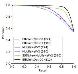
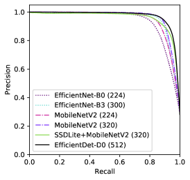
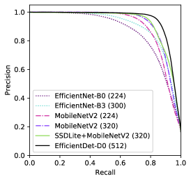
Taking into account that the confidence threshold can be adjusted to avoid nonempty images discarding, we decided to use the precision-recall curve as a graphical tool to compare the general performance of the models considering all possible thresholds. To compare the models effectiveness when discarding empty images, i.e., the true negative rate (TNR), the confidence threshold of each model was adjusted so that the recall for nonempty images was set to 96% – a value reached by models investigated in [13].

(a) Caltech

(b) SS-Site

(c) SS-Time

Figure 1: Precision-recall curve for the nonempty class. Detectors reached higher performances, with wider advantage on the Caltech dataset. Best viewed in color.

		Caltech			SS-Site			SS-Time
Model	CPU	Precision	TNR	Thresh.	Precision	TNR	Thresh.	Precision	TNR	Thresh.
Efficientnet-B0	801ms	60.26%	25.50%	0.355	50.32%	63.00%	0.153	33.08%	61.90%	0.159
Efficientnet-B3	3205ms	56.42%	12.75%	0.305	57.21%	71.97%	0.155	39.27%	70.87%	0.170
MobileNetV2-224	324ms	58.60%	20.18%	0.228	57.72%	72.55%	0.188	30.51%	57.11%	0.126
MobileNetV2-320	638ms	58.58%	20.13%	0.239	62.84%	77.84%	0.191	35.74%	66.13%	0.147
SSDLite+MNetV2	838ms	67.03%	44.42%	0.166	75.32%	87.72%	0.167	47.14%	78.89%	0.147
Efficientdet-D0	4686ms	73.31%	58.86%	0.148	79.14%	90.12%	0.150	47.35%	79.06%	0.143

Table 5: Comparison of precision for the nonempty class and the true negative rate (TNR) where the confidence threshold of each model was adjusted to achieve a recall of 96% on the nonempty class. The reported CPU latency corresponds to the Caltech dataset, but it is similar to the others, being calculated from the average of 50 runs. The true negative rate indicates the percentage of images without animals that would no longer be stored unnecessarily.

(a) EffNet-B0: 0.70, EffNet-B3: 0.67, MNetV2-224: 0.73, MNetV2-320: 0.60, SSDLite: 0.11, EffDet-D0: 0.13

(b) EffNet-B0: 0.42, EffNet-B3: 0.57, MNetV2-224: 0.12, MNetV2-320: 0.80, SSDLite: 0.16, EffDet-D0: 0.10

(c) EffNet-B0: 0.99, EffNet-B3: 0.99, MNetV2-224: 0.99, MNetV2-320: 0.99, SSDLite: 0.87, EffDet-D0: 0.88

(d) EffNet-B0: 0.13, EffNet-B3: 0.03, MNetV2-224: 0.29, MNetV2-320: 0.31, SSDLite: 0.15, EffDet-D0: 0.05

(e) EffNet-B0: 0.99, EffNet-B3: 0.99, MNetV2-224: 0.99, MNetV2-320: 0.99, SSDLite: 0.90, EffDet-D0: 0.94

(f) EffNet-B0: 0.22, EffNet-B3: 0.66, MNetV2-224: 0.48, MNetV2-320: 0.91, SSDLite: 0.77, EffDet-D0: 0.70

Figure 2: Sample classification results reached by the investigated models highlighting their confidence for the nonempty class. The top row depicts images from the Caltech dataset and the bottom row from the Snapshot Serengeti dataset. The first column depicts instances of the empty class while the remainder are nonempty images with the animals highlighted.

We used a Raspberry Pi 3 model B running Raspbian GNU/Linux 10 as a reference edge device to assess the models’ latency. The models were converted to the TensorFlow Lite format without quantization and their latency was calculated using the native benchmark tool provided by TensorFlow. The reported latency values were calculated as the average over 50 runs for each model. Additionally, we also evaluate the models version obtained as a result of post-training quantization [7]. In this scenario, a subset of 500 training instances was employed to calibrate the operations to work with the integer type, while maintaining model inputs and outputs as floating point to keep the original model interface.

4 Experimental Results

4.1 Classifiers vs. Detectors

In order to compare the performance of classifiers and detectors as fairly as possible, the models were trained using subsets composed by instances of the nonempty class annotated with bounding boxes. Despite of the fact that these subsets were generated using a much smaller amount of the total images available for classification, leading to possible sub-optimal models, this number of instances can provide a more realistic perspective of the problem. Indeed, as pointed out by Schneider et al. [17], the vast majority of small-scale research projects focused on camera trap do not have a large amount of labeled images.

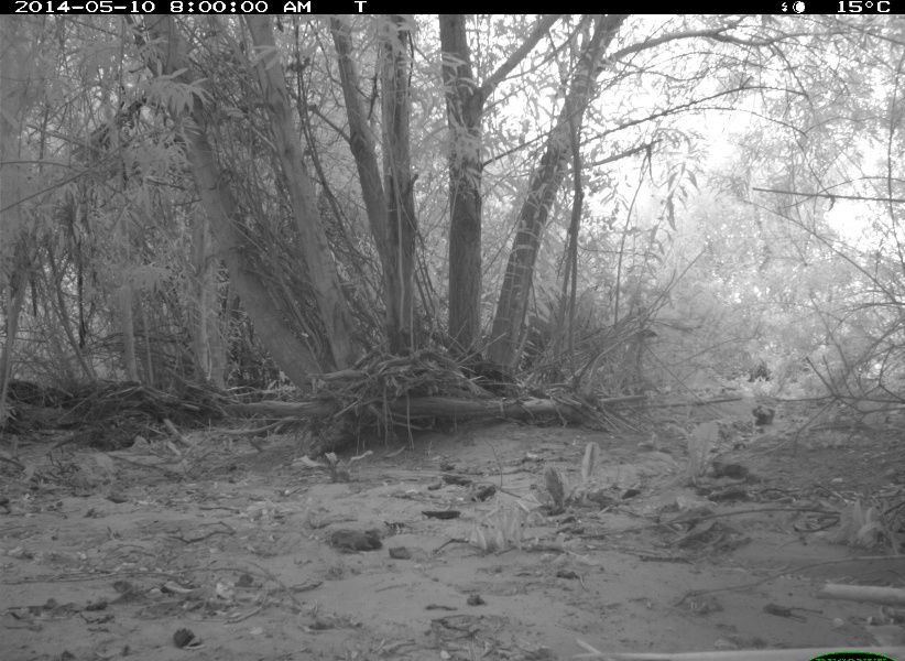
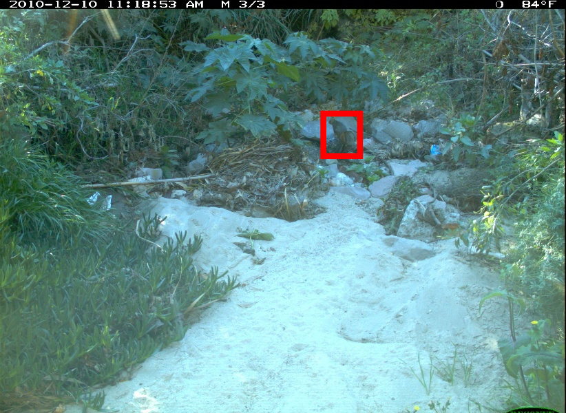
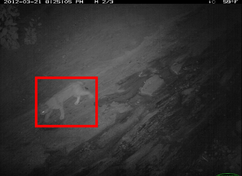
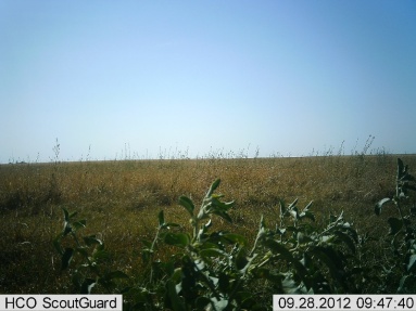
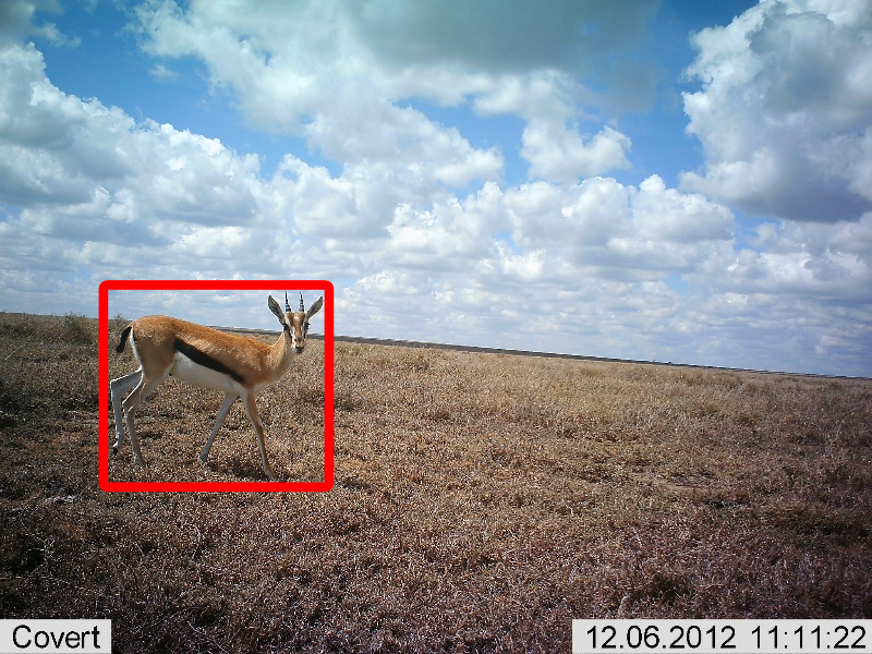
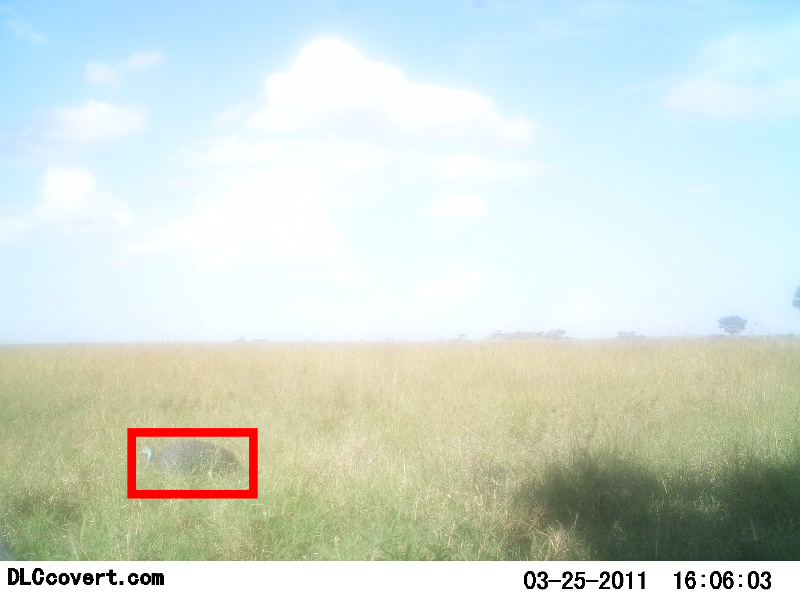
Results: Figure 1 shows the precision-recall curves of the investigated models for each dataset. As expected, detectors outperformed classifiers in all datasets, especially Caltech. Considering a confidence threshold producing 96% of recall, EfficientDet-D0 was able to eliminate more than twice as many empty images when compared to the classifiers using Caltech dataset. In terms of SSDLite+MobileNetV2, it also obtained a significantly higher true negative rate (at least 19% in absolute values), as reported in Table 5. The scenario is quite similar for the Snapshot Serengeti dataset, since detectors also outperformed classifiers by a significant margin (at least 8% of precision). Figure 2 shows some images to illustrate the results attained in our experiments.

(a) SS-Site

(b) SS-Time

Figure 3: Precision-recall curve for the nonempty class of classifiers trained in sets with ten times more images from the SS dataset. The curves of the detectors refer to the models trained on the original smaller set. Best viewed in color.

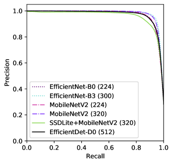
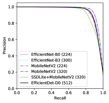
The poor classifier performance on the Caltech dataset can be due to several factors, such as the low variability of backgrounds, the size of animals, camouflage, quality of images, among others. However, our experiments were not designed to identify these nuances intrinsic to this dataset. On the other hand, this may be an interesting topic to be investigated in future work.

Latency-precision trade-off: Table 5 shows the latency for the inference of each model. Although EfficientDet-D0 offers a strong baseline for the problem, its latency is more than four seconds, which is prohibitive because camera trap images are usually obtained within one second between them. In this context, SSDLite+MobileNetV2 may be deemed to attain superior performance since its latency is below one second and it eliminated at least 10% more images than the classifiers with comparable latencies.

4.2 Training with more Images

A common way to improve model performance is to use more training instances [8]. Following this strategy, an experiment was carried out to train the classifiers using the subsets of the SS dataset. This dataset contains ten times more images than the one used in the previous experiment. Figure 3 and Table 6 summarize the results attained in this scenario. The results indicate that classifiers outperformed detectors. We can highlight that MobileNetV2 (224) reached performance similar to SSDLite+MobileNetV2, with less than half of inference latency though. It is important to note, however, that all detectors were trained using data subsets from the previous experiment. Therefore, in order to provide a fair comparison, a similar amount of training instances used to train the classifiers should be used to train the detectors. On the other hand, obtaining more annotated instances for the detection problem is expensive. This is the reason we do not show results using the same dataset for training classifiers and detectors. However, we can conclude based on the results obtained in this experiment that, depending on the number of labeled instances available, classifiers can be a viable option for the problem of identifying empty images, also showing better efficiency in terms of computational resources.

	SS-Site		SS-Time
Model	Precision	TNR	Precision	TNR
Efficientnet-B0	73.92%	86.78%	48.81%	80.25%
Efficientnet-B3	87.67%	94.73%	64.28%	89.54%
MNetV2-224	75.18%	87.63%	49.12%	80.50%
MNetV2-320	82.89%	92.26%	58.61%	86.70%

Table 6: Comparison of precision for the nonempty class and the true negative rate (TNR), with a recall at 96%, for classifiers trained in sets with ten times more images from the SS dataset. Note the significant improvement in the performance of the classifiers, exceeding by a large margin the detectors trained in the original set.

(a) SS-Site

(b) SS-Time

Figure 4: Latency vs. area under the precision-recall curve (PR AUC) for various versions of MobileNetV2 in the SS. The results refer to the models converted to TensorFlow Lite (floating point and integer) and evaluated in a subset of 5,000 test instances. Best viewed in color.

4.3 Model Optimization

				SS-Site		SS-Time
Model		CPU	Memory	Precision	TNR	Precision	TNR
MobileNetV2-224	Float	322ms	22.7MB	58.20%	73.07%	25.67%	45.33%
	Int8	237ms	9.3MB	55.52%	69.99%	26.18%	46.74%
	Int8 (quant aware)	239ms	9.8MB	57.31%	72.10%	-	-
MobileNetV2-0.50-320	Float	259ms	19.7MB	54.86%	69.15%	27.76%	50.86%
	Int8	237ms	9.6MB	51.50%	64.70%	26.67%	48.09%
MobileNetV2-0.75-320	Float	484ms	19.8MB	64.89%	79.72%	31.37%	58.71%
	Int8	408ms	13.3MB	59.50%	74.49%	30.44%	56.87%
	Int8 (quant aware)	413ms	13.4MB	61.38%	76.41%	-	-
MobileNetV2-320	Float	635ms	33.5MB	66.65%	81.25%	30.34%	56.65%
	Int8	485ms	13.9MB	66.70%	81.28%	30.98%	57.95%
SSDLite+MobileNetV2	Float	840ms	31.7MB	73.68%	86.62%	39.50%	71.09%
	Int8	575ms	13.6MB	36.83%	35.72%	19.27%	20.90%

Table 7: Performance comparison of MobileNetV2 models for various widths on the SS dataset. The models were converted to TensorFlow Lite and evaluated using a sample of 5,000 instances randomly chosen from the validation set.

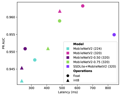
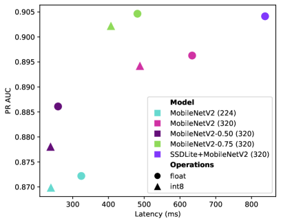
It is possible to observe from results shown in previous sections that models dealing with higher image input resolutions achieved higher performance but at the expense of greater inference latency. In order to reduce latency of these models, we performed an experiment using the SS dataset and MobileNetV2 (320). In this experiment, the number of filters was reduced by adjusting the alpha parameter. We also evaluated the post-training quantization of the models. Since the swish activation function used by EfficientNets is not very well supported for quantization [26], models of this family were not used here. In addition, models evaluation was carried out on a sample of 5,000 instances obtained from the validation set, because the TensorFlow Lite quantized models are not optimized for inference on x86 architectures and graphics cards used for training.

The results shown in Figure 4 reinforce the role of input resolution, since a MobileNetV2 with half the filters (MobileNetV2-0.50) but higher resolution (320) obtained overall performance superior to the performance of the standard model (MobileNetV2 (224)). In Table 7, we may observe that it is possible to reduce about 23% of model latency due to both quantization (SS-site) and number of filters reduction (SS-time), maintaining compatible performance. It is worth mentioning that the quantized version of the SSDLite + MobileNetV2 detector did not obtain good results at the 96% recall level used. These results indicate the importance of assessing the performance of the models after quantization, especially when the confidence threshold is adjusted at certain levels. One way to avoid this problem would be quantization-aware training.

To assess this, we fine tuned the models MobileNetV2-224 and MobileNetV2-0.75-320 trained on SS-Site using quantization-aware training for 2 epochs with the initial learning rate divided by 10. In this case, we were able to improve the results of the quantized versions, as shown in Table 7. Unfortunately, we were not able to assess SSDLite in the same way due to the fact that Tensorflow Object Detection API did not support quantization-aware training for TF2 at the experiments’ time.

Although the focus of this work is the latency-precision trade-off, we also measured the memory usage of each model, as shown in Table 7. Quantized models have a significant reduction in memory usage compared to the floating point models. However, when observed the amount of RAM available on Raspberry Pi (1GB), the memory required by the most complex model is very low (33.5MB), therefore, not affecting the performance of other processes that may be running on the device.

5 Conclusion

In this work, we presented a comparative study between detection and classification models in the context of identification of nonempty images of animals on edge devices. Our results showed that detection models outperform classifiers when both are trained using the same training set, but their superior inference latency can limit their use on edge devices. Moreover, depending on the dataset, it is possible to train classifiers to obtain satisfactory results, especially when there is massive number of images available, as in the Snapshot Serengeti dataset. When detector is essential, e.g. Caltech dataset, but the model’s latency is not within the design requirements, it may be necessary to use hardware accelerators, such as EdgeTPUs or DSPs. Another limitation to detectors is the difficulty on obtaining new instances annotated with bounding boxes, which is time-consuming and expensive. In this situation, one possibility is to use techniques tackling few or no labels, such as semi-supervised learning and self-supervised learning. Other alternative is training an agnostic detection model designed to run on edge devices, inspired by MegaDetector. Regarding the optimization strategies evaluated, the post-training quantization proved to be effective, but it requires a careful evaluation of the resulting model, which may decrease its performance due to the quantization process. However, quantization-aware training may solve this issue. Finally, using models with fewer filters but with higher resolution was also effective. Therefore, techniques such as knowledge distillation and model pruning are interesting directions for future work.

Acknowledgements: This research, according to Article 48 of Decree nº 6.008/2006, was partially funded by Samsung Electronics of Amazonia Ltda, under the terms of Federal Law nº 8.387/1991, through agreement nº 003/2019, signed with ICOMP/UFAM. This study was supported by the Foundation for Research Support of the State of Amazonas (FAPEAM) - POSGRAD Project, and the Coordination for the Improvement of Higher Education Personnel - Brazil (CAPES) - Finance Code 001. The funders had no role in study design, data collection and analysis, decision to publish, or preparation of the manuscript.

References

- [1] Sara Beery, Dan Morris, Siyu Yang, Marcel Simon, Arash Norouzzadeh, and Neel Joshi. Efficient pipeline for automating species id in new camera trap projects. Biodiversity Information Science and Standards, 3:e37222, 2019.
- [2] Sara Beery, Grant Van Horn, and Pietro Perona. Recognition in terra incognita. In Proceedings of the European Conference on Computer Vision, pages 456–473, 2018.
- [3] Ekin D Cubuk, Barret Zoph, Jonathon Shlens, and Quoc V Le. Randaugment: Practical automated data augmentation with a reduced search space. In Proceedings of the IEEE/CVF Conference on Computer Vision and Pattern Recognition Workshops, pages 702–703, 2020.
- [4] Andy Rosales Elias, Nevena Golubovic, Chandra Krintz, and Rich Wolski. Where’s the bear?-automating wildlife image processing using iot and edge cloud systems. In 2017 IEEE/ACM Second Inter. Conf. on Internet-of-Things Design and Implementation (IoTDI), pages 247–258, 2017.
- [5] Tong He, Zhi Zhang, Hang Zhang, Zhongyue Zhang, Junyuan Xie, and Mu Li. Bag of tricks for image classification with convolutional neural networks. In Proceedings of the IEEE/CVF Conference on Computer Vision and Pattern Recognition, pages 558–567, 2019.
- [6] Jonathan Huang, Vivek Rathod, Chen Sun, Menglong Zhu, Anoop Korattikara, Alireza Fathi, Ian Fischer, Zbigniew Wojna, Yang Song, Sergio Guadarrama, et al. Speed/accuracy trade-offs for modern convolutional object detectors. In Proceedings of the IEEE conference on computer vision and pattern recognition, pages 7310–7311, 2017.
- [7] Benoit Jacob, Skirmantas Kligys, Bo Chen, Menglong Zhu, Matthew Tang, Andrew Howard, Hartwig Adam, and Dmitry Kalenichenko. Quantization and training of neural networks for efficient integer-arithmetic-only inference. In Proceedings of the IEEE Conference on Computer Vision and Pattern Recognition, pages 2704–2713, 2018.
- [8] Alexander Kolesnikov, Lucas Beyer, Xiaohua Zhai, Joan Puigcerver, Jessica Yung, Sylvain Gelly, and Neil Houlsby. Big transfer (bit): General visual representation learning. In European conference on computer vision, pages 491–507. Springer, 2020.
- [9] Lila.science. Caltech camera traps. http://lila.science/datasets/caltech-camera-traps. Accessed: 2021-02-17.
- [10] Lila.science. Snapshot serengeti. http://lila.science/datasets/snapshot-serengeti. Accessed: 2021-02-17.
- [11] Tsung-Yi Lin, Michael Maire, Serge Belongie, James Hays, Pietro Perona, Deva Ramanan, Piotr Dollár, and C Lawrence Zitnick. Microsoft coco: Common objects in context. In Eur. conf. on computer vision, pages 740–755. Springer, 2014.
- [12] Wei Liu, Dragomir Anguelov, Dumitru Erhan, Christian Szegedy, Scott Reed, Cheng-Yang Fu, and Alexander C Berg. Ssd: Single shot multibox detector. In European conference on computer vision, pages 21–37. Springer, 2016.
- [13] Mohammad Sadegh Norouzzadeh, Anh Nguyen, Margaret Kosmala, Alexandra Swanson, Meredith S Palmer, Craig Packer, and Jeff Clune. Automatically identifying, counting, and describing wild animals in camera-trap images with deep learning. Proceedings of the National Academy of Sciences, 115(25):E5716–E5725, 2018.
- [14] Shaoqing Ren, Kaiming He, Ross Girshick, and Jian Sun. Faster r-cnn: Towards real-time object detection with region proposal networks. In Advances in neural information processing systems, pages 91–99, 2015.
- [15] Olga Russakovsky, Jia Deng, Hao Su, Jonathan Krause, Sanjeev Satheesh, Sean Ma, Zhiheng Huang, Andrej Karpathy, Aditya Khosla, Michael Bernstein, Alexander C. Berg, and Li Fei-Fei. ImageNet Large Scale Visual Recognition Challenge. International Journal of Computer Vision (IJCV), 115(3):211–252, 2015.
- [16] Mark Sandler, Andrew Howard, Menglong Zhu, Andrey Zhmoginov, and Liang-Chieh Chen. Mobilenetv2: Inverted residuals and linear bottlenecks. In Proceedings of the IEEE conference on computer vision and pattern recognition, pages 4510–4520, 2018.
- [17] Stefan Schneider, Saul Greenberg, Graham W Taylor, and Stefan C Kremer. Three critical factors affecting automated image species recognition performance for camera traps. Ecology and Evolution, 10(7):3503–3517, 2020.
- [18] AB Swanson, M Kosmala, CJ Lintott, RJ Simpson, A Smith, and C Packer. Data from: Snapshot serengeti, high-frequency annotated camera trap images of 40 mammalian species in an african savanna, 2015.
- [19] Michael A Tabak, Mohammad S Norouzzadeh, David W Wolfson, Steven J Sweeney, Kurt C VerCauteren, Nathan P Snow, Joseph M Halseth, Paul A Di Salvo, Jesse S Lewis, Michael D White, et al. Machine learning to classify animal species in camera trap images: Applications in ecology. Meth. in Ecology and Evolution, 10(4):585–590, 2019.
- [20] Mingxing Tan and Quoc Le. Efficientnet: Rethinking model scaling for convolutional neural networks. In Int. Conference on Machine Learning, pages 6105–6114, 2019.
- [21] Mingxing Tan, Ruoming Pang, and Quoc V Le. Efficientdet: Scalable and efficient object detection. In Proceedings of the IEEE/CVF Conference on Computer Vision and Pattern Recognition, pages 10781–10790, 2020.
- [22] TEAM Network. Terrestrial vertebrate protocol implementation manual, v. 3.1, 2011. Tropical Ecology, Assessment and Monitoring Network, Center for Applied Biodiversity Science, Conservation International, Arlington, VA, USA.
- [23] Amanda Tydén and Sara Olsson. Edge machine learning for animal detection, classification, and tracking. Master’s thesis, Linköping University, 2020.
- [24] Alexander Gomez Villa, Augusto Salazar, and Francisco Vargas. Towards automatic wild animal monitoring: Identification of animal species in camera-trap images using very deep convolutional neural networks. Ecological informatics, 41:24–32, 2017.
- [25] Marco Willi, Ross T Pitman, Anabelle W Cardoso, Christina Locke, Alexandra Swanson, Amy Boyer, Marten Veldthuis, and Lucy Fortson. Identifying animal species in camera trap images using deep learning and citizen science. Methods in Ecology and Evolution, 10(1):80–91, 2019.
- [26] Yunyang Xiong, Hanxiao Liu, Suyog Gupta, Berkin Akin, Gabriel Bender, Pieter-Jan Kindermans, Mingxing Tan, Vikas Singh, and Bo Chen. Mobiledets: Searching for object detection architectures for mobile accelerators. arXiv preprint arXiv:2004.14525, 2020.
- [27] Imran A Zualkernan, Salam Dhou, Jacky Judas, Ali Reza Sajun, Brylle Ryan Gomez, Lana Alhaj Hussain, and Dara Sakhnini. Towards an iot-based deep learning architecture for camera trap image classification. In 2020 IEEE Global Conference on Artificial Intelligence and Internet of Things (GCAIoT), pages 1–6. IEEE, 2020.