Contrastive Out-of-Distribution Detection for Pretrained Transformers

Abstract

Pretrained Transformers achieve remarkable performance when training and test data are from the same distribution. However, in real-world scenarios, the model often faces out-of-distribution (OOD) instances that can cause severe semantic shift problems at inference time. Therefore, in practice, a reliable model should identify such instances, and then either reject them during inference or pass them over to models that handle another distribution. In this paper, we develop an unsupervised OOD detection method, in which only the in-distribution (ID) data are used in training. We propose to fine-tune the Transformers with a contrastive loss, which improves the compactness of representations, such that OOD instances can be better differentiated from ID ones. These OOD instances can then be accurately detected using the Mahalanobis distance in the model’s penultimate layer. We experiment with comprehensive settings and achieve near-perfect OOD detection performance, outperforming baselines drastically. We further investigate the rationales behind the improvement, finding that more compact representations through margin-based contrastive learning bring the improvement. We release our code to the community for future research.

1 Introduction

Many natural language classifiers are developed based on a closed-world assumption, i.e., the training and test data are sampled from the same distribution. However, training data can rarely capture the entire distribution. In real-world scenarios, out-of-distribution (OOD) instances, which come from categories that are not known to the model, can often be present in inference phases. These instances could be misclassified by the model into known categories with high confidence, causing the semantic shift problem Hsu et al. (2020). As a practical solution to this problem in real-world applications, the model should detect such instances, and signal exceptions or transmit to models handling other categories or tasks. Although pretrained Transformers Devlin et al. (2019) achieve remarkable results when intrinsically evaluated on in-distribution (ID) data, recent work Hendrycks et al. (2020) shows that many of these models fall short of detecting OOD instances.

Despite the importance, few attempts have been made for the problem of detecting OOD in NLP tasks. One proposed method is to train a model on both the ID and OOD data and regularize the model to produce lower confidence on OOD instances than ID ones Hendrycks et al. (2018); Larson et al. (2019). However, as the OOD instances reside in an unbounded feature space, their distribution during inference is usually unknown. Hence, it is hard to decide which OOD instances to use in training, let alone that they may not be available in lots of scenarios. Another practiced method for OOD detection is to use the maximum class probability as an indicator Shu et al. (2017); Hendrycks et al. (2020), such that lower values indicate more probable OOD instances. Though easy to implement, its OOD detection performance is far from perfection, as prior studies Dhamija et al. (2018); Liang et al. (2018) show that OOD inputs can often get high probabilities as well.

In this paper, we aim at improving the OOD detection ability of natural language classifiers, in particular, the pretrained Transformers, which have been the backbones of many SOTA NLP systems. For practical purposes, we adopt the setting where only ID data are available during task-specific training. Moreover, we require that the model should maintain classification performance on the ID task data. To this end, we propose a contrastive learning framework for unsupervised OOD detection, which is composed of a contrastive loss and an OOD scoring function. Our contrastive loss aims at increasing the discrepancy of the representations of instances from different classes in the task. During training, instances belonging to the same class are regarded as pseudo-ID data while those of different classes are considered mutually pseudo-OOD data. We hypothesize that increasing inter-class discrepancies can help the model learn discriminative features for ID/OOD distinctions, and therefore help detect true OOD data at inference. We study two versions of the contrastive loss: a similarity-based contrastive loss Sohn (2016); Oord et al. (2018); Chen et al. (2020) and a margin-based contrastive loss. The OOD scoring function maps the representations of instances to OOD detection scores, indicating the likelihood of an instance being OOD. We examine different combinations of contrastive losses and OOD scoring functions, including maximum softmax probability, energy score, Mahalanobis distance, and maximum cosine similarity. Particularly, we observe that OOD scoring based on the Mahalanobis distance Lee et al. (2018b), when incorporated with the margin-based contrastive loss, generally leads to the best OOD detection performance. The Mahalanobis distance is computed from the penultimate layer of Transformers by fitting a class-conditional multivariate Gaussian distribution.

The main contributions of this work are three-fold. First, we propose a contrastive learning framework for unsupervised OOD detection, where we comprehensively study combinations of different contrastive learning losses and OOD scoring functions. Second, extensive experiments on various tasks and datasets demonstrate the significant improvement our method has made to OOD detection for Transformers. Third, we provide a detailed analysis to reveal the importance of different incorporated techniques, which also identifies further challenges for this emerging research topic.

2 Related Work

Out-of-Distribution Detection. Determining whether an instance is OOD is critical for the safe deployment of machine learning systems in the real world Amodei et al. (2016). The main challenge is that the distribution of OOD data is hard to estimate a priori. Based on the availability of OOD data, recent methods can be categorized into supervised, self-supervised, and unsupervised ones. Supervised methods train models on both ID and OOD data, where the models are expected to output a uniform distribution over known classes on OOD data Lee et al. (2018a); Dhamija et al. (2018); Hendrycks et al. (2018). However, it is hard to assume the presence of a large dataset that provides comprehensive coverage for OOD instances in practice. Self-supervised methods Bergman and Hoshen (2020) apply augmentation techniques to change certain properties of data (e.g., through rotation of an image) and simultaneously learn an auxiliary model to predict the property changes (e.g., the rotation angle). Such an auxiliary model is expected to have worse generalization on OOD data which can in turn be identified by a larger loss. However, it is hard to define such transformations for natural language. Unsupervised methods use only ID data in training. They detect OOD data based on the class probabilities Bendale and Boult (2016); Hendrycks and Gimpel (2017); Shu et al. (2017); Liang et al. (2018) or other latent space metrics Liu et al. (2020); Lee et al. (2018b). Particularly, Vyas et al. (2018) randomly split the training classes into two subsets and treat them as pseudo-ID and pseudo-OOD data, respectively. They then train an OOD detector that requires the entropy of probability distribution on pseudo-OOD data to be lower than pseudo-ID data. This process is repeated to obtain multiple OOD detectors, and their ensemble is used to detect the OOD instances. This method conducts OOD detection at the cost of high computational overhead in training redundant models and has the limitation of not supporting the detection for binary classification tasks.

Though extensively studied for computer vision (CV), OOD detection has been overlooked in NLP, and most prior works Kim and Kim (2018); Hendrycks et al. (2018); Tan et al. (2019) require both ID and OOD data in training. Hendrycks et al. (2020) use the maximum softmax probability as the detection score and show that pretrained Transformers exhibit better OOD detection performance than models such as LSTM Hochreiter and Schmidhuber (1997), while the performance is still imperfect. Our framework, as an unsupervised OOD detection approach, significantly improves the OOD detection of Transformers only using ID data.

Contrastive Learning. Recently, contrastive learning has received a lot of research attention. It works by mapping instances of the same class into a nearby region and make instances of different classes uniformly distributed Wang and Isola (2020). Many efforts on CV Misra and Maaten (2020); He et al. (2020); Chen et al. (2020) and NLP Giorgi et al. (2021) incorporate contrastive learning into self-supervised learning, which seeks to gather the representations of different augmented views of the same instance and separate those of different instances. Prior work on image classification Tack et al. (2020); Winkens et al. (2020) shows that model trained with self-supervised contrastive learning generates discriminative features for detecting distributional shifts. However, such methods heavily rely on data augmentation of instances and are hard to be applied to NLP. Other efforts on CV Khosla et al. (2020) and NLP Gunel et al. (2021) conduct contrastive learning in a supervised manner, which aims at embedding instances of the same class closer and separating different classes. They show that models trained with supervised contrastive learning exhibit better classification performance. To the best of our knowledge, we are the first to introduce supervised contrastive learning to OOD detection. Such a method does not rely on data augmentation, thus can be easily adapted to existing NLP models. We also propose a margin-based contrastive objective that greatly outperforms standard supervised contrastive losses.

3 Method

In this section, we first formally define the OOD detection problem (Section 3.1), then introduce the overall framework (Section 3.2), and finally present the contrastive representation learning and scoring functions (Section 3.3 and Section 3.4).

3.1 Problem Definition

We aim at improving the OOD detection performance of natural language classifiers that are based on pretrained Transformers, using only ID data in the main-task training. Generally, the out-of-distribution (OOD) instances can be defined as instances $(\bm{x},y)$ sampled from an underlying distribution other than the training distribution $\mathrm{P}(\mathcal{X}_{\text{train}},\mathcal{Y}_{\text{train}})$, where $\mathcal{X}_{\text{train}}$ and $\mathcal{Y}_{\text{train}}$ are the training corpus and training label set, respectively. In this context, literature further divides OOD data into those with semantic shift or non-semantic shift Hsu et al. (2020). Semantic shift refers to the instances that do not belong to $\mathcal{Y}_{\text{train}}$. More specifically, instances with semantic shift may come from unknown categories or irrelevant tasks. Therefore, the model is expected to detect and reject such instances (or forward them to models handling other tasks), instead of mistakenly classifying them into $\mathcal{Y}_{\text{train}}$. Non-semantic shift, on the other hand, refers to the instances that belong to $\mathcal{Y}_{\text{train}}$ but are sampled from a distribution other than $\mathcal{X}_{\text{train}}$, e.g., a different corpus. Though drawn from OOD, those instances can be classified into $\mathcal{Y}_{\text{train}}$, thus can be accepted by the model. Hence, in the context of this paper, we primarily consider an instance $(\bm{x},y)$ to be OOD if $y\notin\mathcal{Y}_{\text{train}}$, i.e., exhibiting semantic shift, to be consistent with the problem settings of prior studies Hendrycks and Gimpel (2017); Lee et al. (2018b); Hendrycks et al. (2020).

We hereby formally define the OOD detection task. Specifically, given a main task of natural language classification (e.g., sentence classification, NLI, etc.), for an instance $\bm{x}$ to be classified, our goal is to develop an auxiliary OOD scoring function $f(\bm{x}):\mathcal{X}\rightarrow\mathbb{R}$. This function should return a low score for an ID instance where $y\in\mathcal{Y}_{\text{train}}$, and a high score for an OOD instance where $y\notin\mathcal{Y}_{\text{train}}$ ($y$ is the underlying label for $\bm{x}$ and is unknown at inference). During inference, we can set a threshold for the OOD score to filter out most OOD instances. This process involves a trade-off between false negative and false positive and may be specific to the application. Meanwhile, we expect that the OOD detection auxiliary should not negatively affect the performance of the main task on ID data.

3.2 Framework Overview

Next, we introduce the formation of our contrastive learning framework for OOD detection. We decompose OOD detection into two steps. The first step is contrastive representation learning, where we focus on learning a representation space $\mathcal{H}$ where the distribution of ID and that of OOD data are distinct. Accordingly, we need another function to map the representation to an OOD score. This process is equivalent to expressing OOD detection as $f(\bm{x})=g(\bm{h})$, where $\bm{h}\in\mathcal{H}$ is the dense representation of the input text $\bm{x}$ given by an encoder, $g:\mathcal{H}\rightarrow\mathbb{R}$ is a scoring function mapping the representation to an OOD detection score. Using this decomposition, we can use different training strategies for $\bm{h}$ and different functions for $g$, which are studies in the following sections.

Input: ID training set $\mathcal{D}_{\text{train}}$ and ID validation set $\mathcal{D}_{\text{val}}$.

Output: A trained classifier and an OOD detector.

Initialize the pretrained Transformer $M$.

for $t=1...T$ do

       Sample a batch from $\mathcal{D}_{\text{train}}$.

       Calculate the classification loss $\mathcal{L}_{\text{ce}}$.

       Calculate the contrastive loss $\mathcal{L}_{\text{cont}}$ as either $\mathcal{L}_{\text{scl}}$ or $\mathcal{L}_{\text{margin}}$

       $\mathcal{L}$ = $\mathcal{L}_{\text{ce}}$ + $\lambda\mathcal{L}_{\text{cont}}$.

       Update model parameters w.r.t. $\mathcal{L}$.

       if $t\;{\%}\;\text{evaluation steps}=0$  then

             Fit the OOD detector on $\mathcal{D}_{\text{val}}$.

             Evaluate both the classifier and OOD detector on $\mathcal{D}_{\text{val}}$.

            

Return the best model checkpoint.

Algorithm 1 Learning Process

The learning process of our framework is described in Algorithm 1. In the training phase, our framework takes training and validation datasets that are both ID as input. The model is optimized with both the (main task) classification loss and the contrastive loss on batches sampled from ID training data. The best model is selected based on the ID validation data. Specifically, for a distribution-based OOD scoring function such as the Mahalanobis distance, we first need to fit the OOD detector on the ID validation data. We then evaluate the trained model on the ID validation data, where a satisfactory model should have a low contrastive loss and preserve the classification performance. In the end, our framework returns a classifier to handle the main task on ID data and an OOD detector to identify OOD instances at inference.

3.3 Contrastive Representation Learning

In this section, we discuss how to learn distinctive representations for OOD detection. For better OOD detection performance, the representation space $\mathcal{H}$ is supposed to minimize the overlap of the representations of ID and OOD data. In a supervised setting where both ID and OOD data are available in training, it would be easy to obtain such $\mathcal{H}$. For example, Dhamija et al. (2018) train the neural model on both ID and OOD data and require the magnitude of representations of OOD instances to be smaller than ID representations. However, in real-world applications, the distribution of OOD data is usually unknown beforehand. We thus tackle a more general problem setting where the OOD data are assumed unavailable in training (unsupervised OOD detection, introduced below).

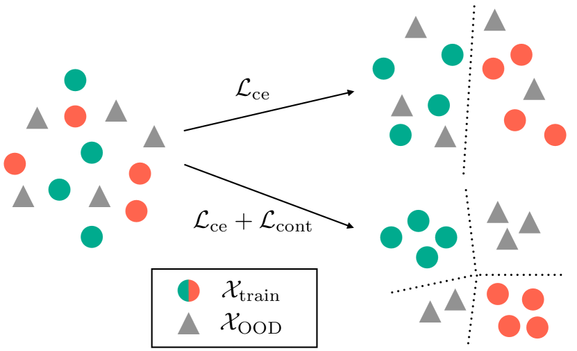
Figure 1: Illustration of our proposed contrastive loss. The contrastive loss seeks to increase the discrepancy of the representations for instances from different training classes, such that OOD instances from unknown classes can be better differentiated.

In this unsupervised setup, though all training data used are ID, they may belong to different classes. We leverage data of distinct classes to learn more discriminative features. Through a contrastive learning objective, instances of the same class form compact clusters, while instances of different classes are encouraged to live apart from each other beyond a certain margin, as illustrated in Figure 1. The discriminative feature space is generalizable to OOD data, which ultimately leads to better OOD detection performance in inference when encountering an unknown distribution. We realize such a strategy using two alternatives of contrastive losses, i.e., the supervised contrastive loss and the margin-based contrastive loss.

Supervised Contrastive Loss. Different from the contrastive loss used in self-supervised representation learning Chen et al. (2020); He et al. (2020) that compares augmented instances to other instances, our contrastive loss contrasts instances to those from different ID classes. To give a more specific illustration of our technique, we first consider the supervised contrastive loss Khosla et al. (2020); Gunel et al. (2021). Specifically, for a multi-class classification problem with $C$ classes, given a batch of training instances $\{(\bm{x}_{i},y_{i})\}_{i=1}^{M}$, where $\bm{x}_{i}$ is the input text, $y_{i}$ is the ground-truth label, the supervised contrastive loss can be formulated as:

$$\mathcal{L}_{\text{scl}}=\sum_{i=1}^{M}\frac{-1}{M|P(i)|}\sum_{p\in P(i)}\log\frac{e^{\bm{z}_{i}^{\intercal}\bm{z}_{p}/\tau}}{\sum\limits_{a\in A(i)}e^{\bm{z}_{i}^{\intercal}\bm{z}_{a}/\tau}},$$

where $A(i)=\{1,...,M\}\backslash\{i\}$ is the set of all anchor instances, $P(i)=\{p\in A(i):y_{i}=y_{p}\}$ is the set of anchor instances from the same class as $i$, $\tau$ is a temperature hyper-parameter, $\bm{z}$ is the L2-normalized [CLS] embedding before the softmax layer Khosla et al. (2020); Gunel et al. (2021). The L2 normalization is for avoiding huge values in the dot product, which may lead to unstable updates. In this case, this loss is optimized to increase the cosine similarity of instance pairs if they are from the same class and decrease it otherwise.

Margin-based Contrastive Loss. The supervised contrastive loss produces minimal gradients when the similarity difference of positive and negative instances exceeds a certain point. However, to better separate OOD instances, it is beneficial to enlarge the discrepancy between classes as much as possible. Therefore, we propose another margin-based contrastive loss. It encourages the L2 distances of instances from the same class to be as small as possible, forming compact clusters, and the L2 distances of instances from different classes to be larger than a margin. Our loss is formulated as:

$$\mathcal{L}_{\text{pos}}=\sum_{i=1}^{M}\frac{1}{|P(i)|}\sum_{p\in P(i)}\|\bm{h}_{i}-\bm{h}_{p}\|^{2},$$

$$\mathcal{L}_{\text{neg}}=\sum_{i=1}^{M}\frac{1}{|N(i)|}\sum_{n\in N(i)}(\xi-\|\bm{h}_{i}-\bm{h}_{n}\|^{2})_{+},$$

$$\mathcal{L}_{\text{margin}}=\frac{1}{dM}\left(\mathcal{L}_{\text{pos}}+\mathcal{L}_{\text{neg}}\right).$$

Here $N(i)=\{n\in A(i):y_{i}\neq y_{n}\}$ is the set of anchor instances from other classes than $y_{i}$, $\bm{h}\in\mathbb{R}^{d}$ is the unnormalized [CLS] embedding before the softmax layer, $\xi$ is a margin, $d$ is the number of dimensions of $\bm{h}$. As we do not use OOD data in training, it is hard to properly tune the margin. Hence, we further incorporate an adaptive margin. Intuitively, distances between instances from the same class should be smaller than those from different classes. Therefore, we define the margin as the maximum distance between pairs of instances from the same class in the batch:

$$\xi=\max_{i=1}^{M}\max_{p\in P(i)}\|\bm{h}_{i}-\bm{h}_{p}\|^{2}.$$

We evaluate both contrastive losses in experiments. In training, the model is jointly optimized with the cross-entropy classification loss $\mathcal{L}_{\text{ce}}$ and the contrastive loss $\mathcal{L}_{\text{cont}}$:

$$\mathcal{L}=\mathcal{L}_{\text{ce}}+\lambda\mathcal{L}_{\text{cont}},$$

where $\lambda$ is a positive coefficient. We tune $\lambda$ based on the contrastive loss and the classification performance on the ID validation set, where a selected value for $\lambda$ should achieve a smaller contrastive loss while maintaining the classification performance.

3.4 OOD Scoring Functions

Next, we introduce the modeling of the OOD scoring function $g$. The goal of the scoring function $g$ is to map the representations of instances to OOD detection scores, where higher scores indicate higher likelihoods for being OOD. In the following, we describe several choices of this scoring function.

Maximum Softmax Probability (MSP). Hendrycks and Gimpel (2017) use the maximum class probability $1-\max_{j=1}^{C}\bm{p}_{j}$ among $C$ training classes in the softmax layer as an OOD indicator. This method has been widely adopted as a baseline for OOD detection Hendrycks and Gimpel (2017); Hsu et al. (2020); Bergman and Hoshen (2020); Hendrycks et al. (2020).

Energy Score (Energy). Liu et al. (2020) interpret the softmax function as the ratio of the joint probability in $\mathcal{X}\times\mathcal{Y}$ to the probability in $\mathcal{X}$, and estimates the probability density of inputs as:

$$g=-\log\sum_{j=1}^{C}\exp(\bm{w}_{j}^{\intercal}\bm{h}),$$

where $\bm{w}_{j}\in\mathbb{R}^{d}$ is the weight of the $j^{th}$ class in the softmax layer, $\bm{h}$ is the input to the softmax layer. A higher $g$ means lower probability density in ID classes and thus implies higher OOD likelihood.

Mahalanobis Distance (Maha). Lee et al. (2018b) model the ID features with class-conditional multivariate Gaussian distributions. It first fits the Gaussian distributions on the ID validation set $\mathcal{D}_{\text{val}}=\{(\bm{x}_{i},y_{i})\}_{i=1}^{M}$ using the input representation $\bm{h}$ in the penultimate layer of model:

$$\bm{\mu}_{j} =\mathbb{E}_{y_{i}=j}\left[\bm{h}_{i}\right],j=1,...,C,$$

$$\bm{\Sigma} =\mathbb{E}\left[\left(\bm{h}_{i}-\bm{\mu}_{y_{i}}\right)\left(\bm{h}_{i}-\bm{\mu}_{y_{i}}\right)^{\intercal}\right],$$

where $C$ is the number of classes, $\bm{\mu}_{j}$ is the mean vector of classes, and $\bm{\Sigma}$ is a shared covariance matrix of all classes. Then, given an instance $\bm{x}$ during inference, it calculates the OOD detection score as the minimum Mahalanobis distance among the $C$ classes:

$$g=-\min_{j=1}^{C}(\bm{h}-\bm{\mu}_{j})^{\intercal}\bm{\Sigma}^{+}(\bm{h}-\bm{\mu}_{j}),$$

where $\bm{\Sigma^{+}}$ is the pseudo-inverse of $\bm{\Sigma}$. The Mahalanobis distance calculates the probability density of $\bm{h}$ in the Gaussian distribution.

Cosine Similarity can also be incorporated to consider the angular similarity of input representations. To do so, the scoring function returns the OOD score as the maximum cosine similarity of $\bm{h}$ to instances of the ID validation set:

$$g=-\max_{i=1}^{M}\cos(\bm{h},\bm{h}_{i}^{(val)}).$$

The above OOD scoring functions, combined with options of contrastive losses, lead to different variants of our framework. We evaluate each combination in experiments.

4 Experiments

This section presents experimental evaluations of the proposed OOD detection framework. We start by describing experimental datasets and settings (Sections 4.1 and 4.2), followed by detailed results analysis and case studies (Sections 4.3, 4.4 and 4.5).

4.1 Datasets

Previous studies on OOD detection mostly focus on image classification, while few have been made on natural language. Currently, there still lacks a well-established benchmark for OOD detection in NLP. Therefore, we extend the selected datasets by Hendrycks et al. (2020) and propose a more extensive benchmark, where we use different pairs of NLP datasets as ID and OOD data, respectively. The criterion for dataset selection is that the OOD instances should not belong to ID classes. To ensure this, we refer to the label descriptions in datasets and manually inspect samples of instances.

We use the following datasets as alternatives of ID data that correspond to three natural language classification tasks:

• Sentiment Analysis. We include two datasets for this task. SST2 Socher et al. (2013) and IMDB Maas et al. (2011) are both datasets for sentiment analysis, where the polarities of sentences are labeled either positive or negative. For SST2, the train/validation/test splits are provided in the dataset. For IMDB, we randomly sample $10\%$ of the training instances as the validation set. Note that both datasets belong to the same task and are not considered OOD to each other.

• Topic Classification. We use 20 Newsgroup Lang (1995), a dataset for topic classification containing 20 classes. We randomly divide the whole dataset into an 80/10/10 split as the train/validation/test set.

• Question Classification. TREC-10 Li and Roth (2002) classifies questions based on the types of their sought-after answers. We use its coarse version with 6 classes and randomly sample $10\%$ of the training instances as the validation set.

Moreover, for the above three tasks, any pair of datasets for different tasks can be regarded as OOD to each other. Besides, following Hendrycks et al. (2020), we also select four additional datasets solely as the OOD data: concatenations of the premises and respective hypotheses from two NLI datasets RTE Dagan et al. (2005); Bar-Haim et al. (2006); Giampiccolo et al. (2007); Bentivogli et al. (2009) and MNLI Williams et al. (2018), the English source side of Machine Translation (MT) datasets English-German WMT16 Bojar et al. (2016) and Multi30K Elliott et al. (2016). We take the test splits in those datasets as OOD instances in testing. Particularly, for MNLI, we use both the matched and mismatched test sets. For Multi30K, we use the union of the flickr 2016 English test set, mscoco 2017 English test set, and filckr 2018 English test set as the test set. There are several reasons for not using them as ID data: (1) WMT16 and Multi30K are MT datasets and do not apply to a natural language classification problem. Therefore, we cannot train a classifier on these two datasets. (2) The instances in NLI datasets are labeled either as entailment/non-entailment for RTE or entailment/neural/contradiction for MNLI, which comprehensively covers all possible relationships of two sentences. Therefore, it is hard to determine OOD instances for NLI datasets. The statistics of the datasets are shown in Table 1.

Dataset	# train	# dev	# test	# class
SST2	67349	872	1821	2
IMDB	22500	2500	25000	2
TREC-10	4907	545	500	6
20NG	15056	1876	1896	20
MNLI	-	-	19643	-
RTE	-	-	3000	-
Multi30K	-	-	2532	-
WMT16	-	-	2999	-

Table 1: Statistics of the datasets.

AUROC $\uparrow$ / FAR95 $\downarrow$		Avg	SST2	IMDB	TREC-10	20NG
w/o $\mathcal{L}_{\text{cont}}$	MSP	94.1 / 35.0	88.9 / 61.3	94.7 / 40.6	98.1 / 7.6	94.6 / 30.5
	Energy	94.0 / 34.7	87.7 / 63.2	93.9 / 49.5	98.0 / 10.4	96.5 / 15.8
	Maha	98.5 / 7.3	96.9 / 18.3	99.8 / 0.7	99.0 / 2.7	98.3 / 7.3
	Cosine	98.2 / 9.7	96.2 / 23.6	99.4 / 2.1	99.2 / 2.3	97.8 / 10.7
w/ $\mathcal{L}_{\text{scl}}$	$\mathcal{L}_{\text{scl}}$ + MSP	90.4 / 46.3	89.7 / 59.9	93.5 / 48.6	90.2 / 36.4	88.1 / 39.2
	$\mathcal{L}_{\text{scl}}$ + Energy	90.5 / 43.5	88.5 / 64.7	92.8 / 50.4	90.3 / 32.2	90.2 / 26.8
	$\mathcal{L}_{\text{scl}}$ + Maha	98.3 / 10.5	96.4 / 26.6	99.6 / 2.0	99.2 / 1.9	97.9 / 11.6
	$\mathcal{L}_{\text{scl}}$ + Cosine	97.7 / 13.0	95.9 / 28.2	99.2 / 4.2	99.0 / 2.4	96.8 / 17.0
w/ $\mathcal{L}_{\text{margin}}$	$\mathcal{L}_{\text{margin}}$ + MSP	93.0 / 33.7	89.7 / 49.2	93.9 / 46.3	97.6 / 6.5	90.9 / 32.6
	$\mathcal{L}_{\text{margin}}$ + Energy	93.9 / 31.0	89.6 / 48.8	93.4 / 52.1	98.4 / 4.6	94.1 / 18.6
	$\mathcal{L}_{\text{margin}}$ + Maha	99.5 / 1.7	99.9 / 0.6	100 / 0	99.3 / 0.4	98.9 / 6.0
	$\mathcal{L}_{\text{margin}}$ + Cosine	99.0 / 3.8	99.6 / 1.7	99.9 / 0.2	99.0 / 1.5	97.4 / 11.8

Table 2: OOD detection performance (in %) of RoBERTa${}_{\textsc{LARGE}}$ trained on the four ID datasets. Due to space limits, for each of the four training ID dataset, we report the macro average of AUROC and FAR95 on all OOD datasets (check Appendix for full results). Results where the contrastive loss improves OOD detection on both evaluation metrics are highlighted in green.“w/o $\mathcal{L}_{\text{cont}}$+MSP” thereof is the method in Hendrycks et al. (2020).

4.2 Experimental Settings

Evaluation Protocol. We train the model on the training split of each of the four aforementioned ID datasets in turn. In the inference phase, the respective test split of that dataset is used as ID test data, while all the test splits of datasets from other tasks are treated as OOD test data.

We adopt two metrics that are commonly used for measuring OOD detection performance in machine learning research Hendrycks and Gimpel (2017); Lee et al. (2018b): (1) AUROC is the area under the receiver operating characteristic curve, which plots the true positive rate (TPR) against the false positive rate (FPR). A higher AUROC value indicates better OOD detection performance, and a random guessing detector corresponds to an AUROC of $50\%$. (2) FAR95 is the probability for a negative example (OOD) to be mistakenly classified as positive (ID) when the TPR is $95\%$, in which case a lower value indicates better performance. Both metrics are threshold-independent.

Compared Methods. We evaluate all configurations of contrastive losses and OOD scoring functions. Those include 12 settings composed of 3 alternative setups for contrastive losses ($\mathcal{L}_{\text{scl}}$, $\mathcal{L}_{\text{margin}}$ or w/o a contrastive loss) and 4 alternatives of OOD scoring functions (MSP, the energy score, Maha, or cosine similarity).

Model Configuration. We implement our framework upon Huggingface’s Transformers Wolf et al. (2020) and build the text classifier based on RoBERTa${}_{\textsc{LARGE}}$ Liu et al. (2019) in the main experiment. All models are optimized with Adam Kingma and Ba (2015) using a learning rate of $1\mathrm{e}{-5}$, with a linear learning rate decay towards 0. We use a batch size of 32 and fine-tune the model for 10 epochs. When training the model on each training split of a dataset, we use the respective validation split for both hyper-parameter tuning and The hyper-parameters are tuned according to the classification performance and the contrastive loss on the ID validation set. We find that $\tau=0.3$ and $\lambda=2$ work well with $\mathcal{L}_{\text{scl}}$, while $\lambda=2$ work well with $\mathcal{L}_{\text{margin}}$, and we apply them to all datasets.

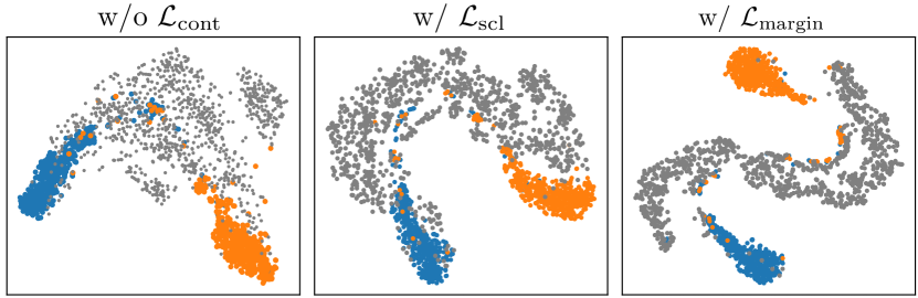
Figure 2: Visualization of the representations for positive, negative instances in SST2 and OOD ones. The discrepancy between ID and OOD representations is greater on representations obtained with $\mathcal{L}_{\text{margin}}$.

4.3 Main Results

We hereby discuss the main results of the OOD detection performance. Note that the incorporation of our OOD techniques does not lead to noticeable interference of the main-task performance, for which an analysis is later given in Section 4.5.

The OOD detection results by different configurations of models are given in Table 2. For all results, we report the average of 5 runs using different random seeds. Each model configuration is reported with separate sets of results when being trained on different datasets, on top of which the macro average performance is also reported. For settings with $\mathcal{L}_{\text{scl}}$ and $\mathcal{L}_{\text{margin}}$, results better than the baselines (w/o a contrastive loss) are marked as red. We observe that: (1) Among OOD detection functions, the Mahalanobis distance performs the best on average and drastically outperforms the MSP baseline used in Hendrycks et al. (2020). This is due to that the Mahalanobis distance can better capture the distributional difference. (2) Considering models trained on different ID datasets, the model variants with $\mathcal{L}_{\text{margin}}$ have achieved near-perfect OOD detection performance on SST2, IMDB, and TREC-10. While on the 20 Newsgroup dataset that contains articles from multiple genres, there is still room for improvement. (3) Overall, The margin-based contrastive loss ($\mathcal{L}_{\text{margin}}$) significantly improves OOD detection performance. Particularly, it performs the best with the Mahalanobis distance, reducing the average FAR95 of Maha by $77\%$ from $7.3\%$ to $1.7\%$. (4) The supervised contrastive loss ($\mathcal{L}_{\text{scl}}$) does not effectively improve OOD detection in general. In many cases, its performance is even worse than the baseline.

AUROC $\uparrow$ / FAR95 $\downarrow$	TREC-10	20NG
MSP	73.7 / 56.5	76.4 / 80.7
Maha	75.5 / 56.1	77.2 / 74.1
$\mathcal{L}_{\text{margin}}$ + MSP	64.1 / 66.4	74.6 / 82.0
$\mathcal{L}_{\text{margin}}$ + Maha	76.6 / 61.3	78.5 / 72.7

Table 3: Novel class detection performance.

4.4 Novel Class Detection

We further evaluate our framework in a more challenging setting of novel class detection. Given a dataset containing multiple classes ($\geq 3$), We randomly reserve one class as OOD data while treating others as ID data. We then train the model on the ID data and require it to identify OOD data in inference. In this case, the OOD data are sampled from the same task corpus as the ID data, and thus is much harder to be distinguished. We report the average performance of 5 trials in Table 3. The results are consistent with the main results in general. The Mahalanobis distance consistently outperforms consistently outperforms MSP, and the $\mathcal{L}_{\text{margin}}$ achieves better performance except for the FAR95 metric on the TREC-10 dataset. However, the performance gain is notably smaller than that in the main experiments. Moreover, none of the compared methods achieve an AUROC score of over $80\%$. This experiment shows that compared to detecting OOD instances from other tasks, detecting OOD instances from similar corpora is much more challenging and remains room for further investigation.

4.5 Analysis

Visualization of Representations. To help understand the increased OOD detection performance of our method, we visualize the penultimate layer of the Transformer trained with different contrastive losses. Specifically, we train the model on SST2 and visualize instances from the SST2 validation set and OOD datasets using t-SNE Van der Maaten and Hinton (2008), as shown in Figure 2. We observe that the representations obtained with $\mathcal{L}_{\text{margin}}$ can distinctly separate ID and OOD instances, such that ID and OOD clusters see almost no overlap.

Main Task Performance. As stated in Section 3.1, the increased OOD detection performance should not interfere with the classification performance on the main task. We evaluate the trained classifier on the four ID datasets. The results are shown in Table 4. We observe that the contrastive loss does not noticeably decrease the classification performance, nor does it increase the performance, which differs from the observations by Gunel et al. (2021).

Accuracy	SST2	IMDB	TREC-10	20NG
w/o $\mathcal{L}_{\text{cont}}$	96.4	95.3	97.7	93.6
w/ $\mathcal{L}_{\text{scl}}$	96.3	95.3	97.4	93.4
w/ $\mathcal{L}_{\text{margin}}$	96.3	95.3	97.5	93.9

Table 4: Accuracy of the trained classifier.

AUROC $\uparrow$ / FAR95 $\downarrow$	L1	Cosine	L2
MSP	93.6 / 31.1	94.1 / 30.9	92.2 / 32.0
Energy	93.8 / 27.2	94.7 / 26.9	94.4 / 27.5
Maha	99.3 / 2.8	99.2 / 3.0	99.4 / 1.7
Cosine	98.1 / 10.9	98.8 / 5.3	99.0 / 3.9

Table 5: Average OOD detection performance of different distance metrics.

Distance Metrics. Besides L2 distance, we further evaluate the L1 distance and the cosine distance with the margin-based contrastive loss $\mathcal{L}_{\text{margin}}$. Results are shown in Table 5. Due to space limitations, we only report the average OOD performance on the four ID datasets. We observe that the three metrics achieve similar performance, and all outperform the baseline when using Maha as the scoring function. Among them, L2 distance gets slightly better OOD detection performance. Moreover, $\mathcal{L}_{\text{margin}}$ significantly outperforms $\mathcal{L}_{\text{scl}}$ when both use cosine as the distance metric. It shows that their performance difference arises from the characteristics of the losses instead of the metric.

AUROC $\uparrow$ / FAR95 $\downarrow$	Maha	Maha + $\mathcal{L}_{\text{margin}}$
BERT${}_{\textsc{BASE}}$	95.7 / 21.5	98.4 / 8.1
BERT${}_{\textsc{LARGE}}$	97.7 / 13.3	99.1 / 3.9
RoBERTa${}_{\textsc{BASE}}$	98.4 / 9.3	99.6 / 2.0
RoBERTa${}_{\textsc{LARGE}}$	98.5 / 7.3	99.4 / 1.7

Table 6: Average OOD detection performance of other pretrained Transformers.

OOD Detection by Other Transformers. We also evaluate the OOD detection ability of other pretrained Transformers in Table 6 and report the average performance on the four ID datasets. For BERT Devlin et al. (2019), we use $\lambda=0.2$. We observe that: (1) Larger models have better OOD detection ability. For both BERT and RoBERTa, the large versions offer better results than the base versions. (2) Pretraining on diverse data improves OOD detection. RoBERTa, which uses more pretraining corpora, outperforms BERT models. (3) The margin-based contrastive loss consistently improves OOD detection on all encoders.

5 Conclusion

This work presents an unsupervised OOD detection framework for pretrained Transformers requiring only ID data. We systematically investigate the combination of contrastive losses and scoring functions, the two key components in our framework. In particular, we propose a margin-based contrastive objective for learning compact representations, which, in combination with the Mahalanobis distance, achieves the best performance: near-perfect OOD detection on various tasks and datasets. We further propose novel class detection as the future challenge for OOD detection.

Ethical Consideration

This work does not present any direct societal consequences. The proposed work seeks to develop a general contrastive learning framework that handles unsupervised OOD detection in natural language classification. We believe this study leads to intellectual merits that benefit with reliable application of NLU models. Since in real-world scenarios, a model may face heterogeneous inputs with significant semantic shifts from its training distributions. And it potentially has broad impacts since the tackled issues also widely exist in tasks of other areas. All experiments are conducted on open datasets.

Appendix A Full Results

We show the full OOD detection performance of ID datasets on OOD datasets. The results of w/o $\mathcal{L}_{\text{cont}}$ and w/ $\mathcal{L}_{\text{margin}}$ are shown in Table 7 and Table 8, respectively.

AUROC	SST2				IMDB				TREC-10				20NG
	MSP	Energy	Maha	Cosine	MSP	Energy	Maha	Cosine	MSP	Energy	Maha	Cosine	MSP	Energy	Maha	Cosine
SST2	-	-	-	-	-	-	-	-	97.1	94.8	97.4	97.9	98.6	99.6	99.4	99.7
IMDB	-	-	-	-	-	-	-	-	98.9	98.8	99.5	99.5	95.9	97.8	98.9	98.6
TREC-10	91.8	91.5	97.8	97.0	94.9	94.0	100	99.5	-	-	-	-	95.1	97.6	98.9	98.7
20NG	93.6	93.4	94.9	93.2	96.0	95.6	99.8	99.6	98.2	99.0	99.5	99.6	-	-	-	-
MNLI	84.6	83.6	95.1	94.6	93.1	92.4	99.5	99.0	97.0	97.3	98.9	98.8	94.1	96.1	98.1	97.5
RTE	89.2	87.4	98.4	98.1	93.9	93.3	99.8	99.5	98.6	98.8	99.5	99.4	90.3	92.8	96.5	95.2
WMT16	84.0	82.4	96.4	95.9	93.4	92.7	99.7	99.1	97.9	98.2	99.4	99.3	92.7	95.0	97.8	96.8
Multi30K	90.2	88.1	98.8	98.6	96.4	95.6	99.9	99.8	99.1	99.2	99.7	99.6	95.7	97.0	98.7	98.3
Avg	88.9	87.7	96.9	96.2	94.7	93.9	99.8	99.4	98.1	98.0	99.0	99.2	94.6	96.5	98.3	97.8

FAR95	SST2				IMDB				TREC-10				20NG
	MSP	Energy	Maha	Cosine	MSP	Energy	Maha	Cosine	MSP	Energy	Maha	Cosine	MSP	Energy	Maha	Cosine
SST2	-	-	-	-	-	-	-	-	14.5	28.5	12.0	6.4	9.0	2.3	0.3	0.9
IMDB	-	-	-	-	-	-	-	-	2.9	4.5	0.2	0.3	25.3	10.5	4.4	6.4
TREC-10	61.3	63.1	13.2	19.4	37.4	57.7	0	1.5	-	-	-	-	35.0	14.9	1.3	8.3
20NG	52.1	52.5	39.5	55.9	28.4	32.1	0.2	0.6	7.2	6.6	0.3	1.0	-	-	-	-
MNLI	68.4	68.7	27.0	31.4	51.4	55.4	2.2	4.8	13.6	15.5	3.2	4.2	36.0	20.2	10.1	13.9
RTE	59.7	62.4	8.0	9.0	49.9	54.7	0.7	1.9	5.2	5.5	0.8	1.4	49.0	30.1	17.1	21.9
WMT16	69.4	70.6	17.2	20.2	50.9	57.6	1.2	3.8	8.5	10.2	1.8	2.2	40.5	23.1	11.9	16.4
Multi30K	57.3	61.7	5.5	6.0	25.7	34.3	0	0.2	1.3	1.8	0.3	0.2	18.9	9.2	5.9	7.0
Avg	61.3	63.2	18.3	23.6	40.6	48.6	0.7	2.1	7.6	10.4	2.7	2.3	30.5	15.8	7.3	10.7

Table 7: AUROC and FAR95 (in %) of RoBERTa${}_{\textsc{LARGE}}$ model trained w/o $\mathcal{L}_{\text{cont}}$. Results are averaged over 5 runs with different seeds.

AUROC	SST2				IMDB				TREC-10				20NG
	MSP	Energy	Maha	Cosine	MSP	Energy	Maha	Cosine	MSP	Energy	Maha	Cosine	MSP	Energy	Maha	Cosine
SST2	-	-	-	-	-	-	-	-	96.2	96.6	98.4	97.8	96.3	98.1	99.5	99.0
IMDB	-	-	-	-	-	-	-	-	99.3	99.7	99.6	99.3	94.5	96.9	99.0	98.4
TREC-10	95.1	94.9	99.5	99.0	93.8	93.3	100	100	-	-	-	-	88.0	92.4	99.6	96.5
20NG	95.2	95.0	100	100	95.4	95.3	100	99.9	99.2	99.8	99.8	99.7	-	-	-	-
MNLI	82.8	82.7	99.8	99.5	92.4	91.7	100	99.9	96.6	97.6	99.2	98.8	91.0	94.2	98.4	97.2
RTE	87.4	87.5	100	99.9	92.9	92.1	100	99.9	96.6	98.1	99.6	99.2	84.5	88.7	98.2	95.6
WMT16	83.9	84.0	99.9	99.4	92.9	92.2	100	99.9	97.1	98.0	99.4	99.1	88.3	92.5	98.5	96.7
Multi30K	93.5	93.6	100	99.9	95.9	95.7	100	100	97.9	98.9	99.5	99.3	93.7	96.0	99.1	98.3
Avg	89.7	89.6	99.9	99.6	93.9	93.4	100	99.9	97.6	98.4	99.3	99.0	90.9	94.1	98.9	97.4

FAR95	SST2				IMDB				TREC-10				20NG
	MSP	Energy	Maha	Cosine	MSP	Energy	Maha	Cosine	MSP	Energy	Maha	Cosine	MSP	Energy	Maha	Cosine
SST2	-	-	-	-	-	-	-	-	11.9	10.4	1.6	6.9	13.7	5.3	1.2	2.6
IMDB	-	-	-	-	-	-	-	-	0.5	0.2	0	0	23.6	11.4	4.7	7.4
TREC-10	35.3	35.0	2.4	4.3	50.0	54.0	0	0	-	-	-	-	27.2	13.8	1.4	4.4
20NG	36.4	36.3	0	0	37.8	33.1	0	0	0.6	0.2	0	0	-	-	-	-
MNLI	64.6	64.3	0.4	2.6	52.2	83.8	0.1	0.9	9.6	6.7	0.7	1.9	37.4	24.7	9.6	16.7
RTE	58.3	57.7	0	0.3	52.9	54.3	0	0.3	9.8	6.2	0.1	0.5	52.9	35.4	11.1	24.2
WMT16	64.3	64.1	0.5	3.0	53.7	55.7	0	0.4	7.9	5.7	0.5	1.3	45.3	27.8	7.5	18.7
Multi30K	36.3	35.4	0	0.3	30.9	31.9	0	0	5.3	2.6	0	0.2	27.8	12.0	6.9	8.7
Avg	49.2	48.8	0.6	1.7	46.3	52.1	0	0.2	6.5	4.6	0.4	1.5	32.6	18.6	6.0	11.8

Table 8: AUROC and FAR95 (in %) of RoBERTa${}_{\textsc{LARGE}}$ model trained w/ $\mathcal{L}_{\text{margin}}$. Results are averaged over 5 runs with different seeds.

References

- Amodei et al. (2016) Dario Amodei, Christopher Olah, J. Steinhardt, P. F. Christiano, John Schulman, and Dandelion Mané. 2016. Concrete problems in ai safety. ArXiv, abs/1606.06565.
- Bar-Haim et al. (2006) Roy Bar-Haim, Ido Dagan, B. Dolan, L. Ferro, Danilo Giampiccolo, and B. Magnini. 2006. The second pascal recognising textual entailment challenge.
- Bendale and Boult (2016) Abhijit Bendale and T. Boult. 2016. Towards open set deep networks. 2016 IEEE Conference on Computer Vision and Pattern Recognition (CVPR), pages 1563–1572.
- Bentivogli et al. (2009) L. Bentivogli, Peter Clark, Ido Dagan, and Danilo Giampiccolo. 2009. The sixth pascal recognizing textual entailment challenge. In TAC.
- Bergman and Hoshen (2020) Liron Bergman and Yedid Hoshen. 2020. Classification-based anomaly detection for general data. In International Conference on Learning Representations, volume abs/2005.02359.
- Bojar et al. (2016) Ondřej Bojar, Rajen Chatterjee, Christian Federmann, Yvette Graham, Barry Haddow, Matthias Huck, Antonio Jimeno Yepes, Philipp Koehn, Varvara Logacheva, Christof Monz, et al. 2016. Findings of the 2016 conference on machine translation. In Proceedings of the First Conference on Machine Translation: Volume 2, Shared Task Papers, pages 131–198.
- Chen et al. (2020) Ting Chen, Simon Kornblith, Mohammad Norouzi, and Geoffrey Hinton. 2020. A simple framework for contrastive learning of visual representations. In International conference on machine learning, pages 1597–1607. PMLR.
- Dagan et al. (2005) Ido Dagan, Oren Glickman, and B. Magnini. 2005. The pascal recognising textual entailment challenge. In MLCW.
- Devlin et al. (2019) Jacob Devlin, Ming-Wei Chang, Kenton Lee, and Kristina Toutanova. 2019. BERT: Pre-training of deep bidirectional transformers for language understanding. In Proceedings of the 2019 Conference of the North American Chapter of the Association for Computational Linguistics: Human Language Technologies, Volume 1 (Long and Short Papers), pages 4171–4186, Minneapolis, Minnesota.
- Dhamija et al. (2018) A. Dhamija, Manuel Günther, and T. Boult. 2018. Reducing network agnostophobia. In NeurIPS.
- Elliott et al. (2016) Desmond Elliott, Stella Frank, Khalil Sima’an, and Lucia Specia. 2016. Multi30K: Multilingual English-German image descriptions. In Proceedings of the 5th Workshop on Vision and Language, pages 70–74, Berlin, Germany. Association for Computational Linguistics.
- Giampiccolo et al. (2007) Danilo Giampiccolo, B. Magnini, Ido Dagan, and W. Dolan. 2007. The third pascal recognizing textual entailment challenge. In ACL-PASCAL@ACL.
- Giorgi et al. (2021) John Giorgi, Osvald Nitski, Bo Wang, and Gary Bader. 2021. DeCLUTR: Deep contrastive learning for unsupervised textual representations. In Proceedings of the 59th Annual Meeting of the Association for Computational Linguistics and the 11th International Joint Conference on Natural Language Processing (Volume 1: Long Papers), pages 879–895, Online. Association for Computational Linguistics.
- Gunel et al. (2021) Beliz Gunel, Jingfei Du, Alexis Conneau, and Ves Stoyanov. 2021. Supervised contrastive learning for pre-trained language model fine-tuning. In International Conference for Learning Representations.
- He et al. (2020) Kaiming He, Haoqi Fan, Yuxin Wu, Saining Xie, and Ross Girshick. 2020. Momentum contrast for unsupervised visual representation learning. In Proceedings of the IEEE/CVF Conference on Computer Vision and Pattern Recognition, pages 9729–9738.
- Hendrycks and Gimpel (2017) Dan Hendrycks and Kevin Gimpel. 2017. A baseline for detecting misclassified and out-of-distribution examples in neural networks. In International Conference on Learning Representations.
- Hendrycks et al. (2020) Dan Hendrycks, Xiaoyuan Liu, Eric Wallace, Adam Dziedzic, Rishabh Krishnan, and Dawn Song. 2020. Pretrained transformers improve out-of-distribution robustness. In Proceedings of the 58th Annual Meeting of the Association for Computational Linguistics, pages 2744–2751, Online.
- Hendrycks et al. (2018) Dan Hendrycks, Mantas Mazeika, and Thomas Dietterich. 2018. Deep anomaly detection with outlier exposure. In International Conference on Learning Representations.
- Hochreiter and Schmidhuber (1997) S. Hochreiter and J. Schmidhuber. 1997. Long short-term memory. Neural Computation, 9:1735–1780.
- Hsu et al. (2020) Yen-Chang Hsu, Yilin Shen, Hongxia Jin, and Z. Kira. 2020. Generalized odin: Detecting out-of-distribution image without learning from out-of-distribution data. 2020 IEEE/CVF Conference on Computer Vision and Pattern Recognition (CVPR), pages 10948–10957.
- Khosla et al. (2020) Prannay Khosla, Piotr Teterwak, Chen Wang, Aaron Sarna, Yonglong Tian, Phillip Isola, Aaron Maschinot, Ce Liu, and Dilip Krishnan. 2020. Supervised contrastive learning. Advances in Neural Information Processing Systems, 33.
- Kim and Kim (2018) Joo-Kyung Kim and Young-Bum Kim. 2018. Joint learning of domain classification and out-of-domain detection with dynamic class weighting for satisficing false acceptance rates. Proc. Interspeech 2018, pages 556–560.
- Kingma and Ba (2015) Diederik P. Kingma and Jimmy Ba. 2015. Adam: A method for stochastic optimization. In International Conference for Learning Representations.
- Lang (1995) Ken Lang. 1995. Newsweeder: Learning to filter netnews. In Machine Learning Proceedings 1995, pages 331–339. Elsevier.
- Larson et al. (2019) Stefan Larson, Anish Mahendran, Joseph J Peper, Christopher Clarke, Andrew Lee, Parker Hill, Jonathan K Kummerfeld, Kevin Leach, Michael A Laurenzano, Lingjia Tang, et al. 2019. An evaluation dataset for intent classification and out-of-scope prediction. In Proceedings of the 2019 Conference on Empirical Methods in Natural Language Processing and the 9th International Joint Conference on Natural Language Processing (EMNLP-IJCNLP), pages 1311–1316.
- Lee et al. (2018a) Kimin Lee, Honglak Lee, Kibok Lee, and Jinwoo Shin. 2018a. Training confidence-calibrated classifiers for detecting out-of-distribution samples. In International Conference on Learning Representations.
- Lee et al. (2018b) Kimin Lee, Kibok Lee, Honglak Lee, and Jinwoo Shin. 2018b. A simple unified framework for detecting out-of-distribution samples and adversarial attacks. In Proceedings of the 32nd International Conference on Neural Information Processing Systems, pages 7167–7177.
- Li and Roth (2002) Xin Li and Dan Roth. 2002. Learning question classifiers. In COLING 2002: The 19th International Conference on Computational Linguistics.
- Liang et al. (2018) Shiyu Liang, Yixuan Li, and R Srikant. 2018. Enhancing the reliability of out-of-distribution image detection in neural networks. In International Conference on Learning Representations.
- Liu et al. (2020) Weitang Liu, Xiaoyun Wang, John Owens, and Yixuan Li. 2020. Energy-based out-of-distribution detection. In Advances in Neural Information Processing Systems, volume 33.
- Liu et al. (2019) Yinhan Liu, Myle Ott, Naman Goyal, Jingfei Du, Mandar Joshi, Danqi Chen, Omer Levy, Mike Lewis, Luke Zettlemoyer, and Veselin Stoyanov. 2019. Roberta: A robustly optimized bert pretraining approach. arXiv preprint arXiv:1907.11692.
- Maas et al. (2011) Andrew L. Maas, Raymond E. Daly, Peter T. Pham, Dan Huang, Andrew Y. Ng, and Christopher Potts. 2011. Learning word vectors for sentiment analysis. In Proceedings of the 49th Annual Meeting of the Association for Computational Linguistics: Human Language Technologies, pages 142–150, Portland, Oregon, USA. Association for Computational Linguistics.
- Misra and Maaten (2020) Ishan Misra and Laurens van der Maaten. 2020. Self-supervised learning of pretext-invariant representations. In Proceedings of the IEEE/CVF Conference on Computer Vision and Pattern Recognition, pages 6707–6717.
- Oord et al. (2018) Aaron van den Oord, Yazhe Li, and Oriol Vinyals. 2018. Representation learning with contrastive predictive coding. arXiv preprint arXiv:1807.03748.
- Shu et al. (2017) Lei Shu, Hu Xu, and Bing Liu. 2017. DOC: Deep open classification of text documents. In Proceedings of the 2017 Conference on Empirical Methods in Natural Language Processing, pages 2911–2916, Copenhagen, Denmark. Association for Computational Linguistics.
- Socher et al. (2013) Richard Socher, Alex Perelygin, Jean Wu, Jason Chuang, Christopher D. Manning, Andrew Ng, and Christopher Potts. 2013. Recursive deep models for semantic compositionality over a sentiment treebank. In Proceedings of the 2013 Conference on Empirical Methods in Natural Language Processing, pages 1631–1642, Seattle, Washington, USA. Association for Computational Linguistics.
- Sohn (2016) Kihyuk Sohn. 2016. Improved deep metric learning with multi-class n-pair loss objective. In Proceedings of the 30th International Conference on Neural Information Processing Systems, pages 1857–1865.
- Tack et al. (2020) Jihoon Tack, Sangwoo Mo, Jongheon Jeong, and Jinwoo Shin. 2020. Csi: Novelty detection via contrastive learning on distributionally shifted instances. In 34th Conference on Neural Information Processing Systems (NeurIPS) 2020. Neural Information Processing Systems.
- Tan et al. (2019) Ming Tan, Yang Yu, Haoyu Wang, Dakuo Wang, Saloni Potdar, Shiyu Chang, and Mo Yu. 2019. Out-of-domain detection for low-resource text classification tasks. In Proceedings of the 2019 Conference on Empirical Methods in Natural Language Processing and the 9th International Joint Conference on Natural Language Processing (EMNLP-IJCNLP), pages 3566–3572, Hong Kong, China.
- Van der Maaten and Hinton (2008) Laurens Van der Maaten and Geoffrey Hinton. 2008. Visualizing data using t-sne. Journal of machine learning research, 9(11).
- Vyas et al. (2018) Apoorv Vyas, Nataraj Jammalamadaka, Xia Zhu, Dipankar Das, Bharat Kaul, and Theodore L Willke. 2018. Out-of-distribution detection using an ensemble of self supervised leave-out classifiers. In Proceedings of the European Conference on Computer Vision (ECCV), pages 550–564.
- Wang and Isola (2020) Tongzhou Wang and Phillip Isola. 2020. Understanding contrastive representation learning through alignment and uniformity on the hypersphere. In International Conference on Machine Learning, pages 9929–9939. PMLR.
- Williams et al. (2018) Adina Williams, Nikita Nangia, and Samuel Bowman. 2018. A broad-coverage challenge corpus for sentence understanding through inference. In Proceedings of the 2018 Conference of the North American Chapter of the Association for Computational Linguistics: Human Language Technologies, Volume 1 (Long Papers), pages 1112–1122, New Orleans, Louisiana. Association for Computational Linguistics.
- Winkens et al. (2020) Jim Winkens, Rudy Bunel, Abhijit Guha Roy, Robert Stanforth, Vivek Natarajan, Joseph R Ledsam, Patricia MacWilliams, Pushmeet Kohli, Alan Karthikesalingam, Simon Kohl, et al. 2020. Contrastive training for improved out-of-distribution detection. arXiv preprint arXiv:2007.05566.
- Wolf et al. (2020) Thomas Wolf, Lysandre Debut, Victor Sanh, Julien Chaumond, Clement Delangue, Anthony Moi, Pierric Cistac, Tim Rault, Remi Louf, Morgan Funtowicz, Joe Davison, Sam Shleifer, Patrick von Platen, Clara Ma, Yacine Jernite, Julien Plu, Canwen Xu, Teven Le Scao, Sylvain Gugger, Mariama Drame, Quentin Lhoest, and Alexander Rush. 2020. Transformers: State-of-the-art natural language processing. In Proceedings of the 2020 Conference on Empirical Methods in Natural Language Processing: System Demonstrations, pages 38–45, Online.