Consistent Accelerated Inference via Confident Adaptive Transformers

Abstract

We develop a novel approach for confidently accelerating inference in the large and expensive multilayer Transformers that are now ubiquitous in natural language processing (NLP). Amortized or approximate computational methods increase efficiency, but can come with unpredictable performance costs. In this work, we present CATs—Confident Adaptive Transformers—in which we simultaneously increase computational efficiency, while guaranteeing a specifiable degree of consistency with the original model with high confidence. Our method trains additional prediction heads on top of intermediate layers, and dynamically decides when to stop allocating computational effort to each input using a meta consistency classifier. To calibrate our early prediction stopping rule, we formulate a unique extension of conformal prediction. We demonstrate the effectiveness of this approach on four classification and regression tasks.

1 Introduction

Large pre-trained language models have become the de facto standard approach for solving natural language processing tasks (Devlin et al., 2019; Liu et al., 2019). Despite their impressive performance, however, their often massive computational burden makes them costly to run (Schwartz et al., 2019; Sharir et al., 2020). Concerns about their efficiency have kindled a large body of research in the field Sanh et al. (2020); Schwartz et al. (2020); Fan et al. (2020). For multilayered architectures such as the Transformer, a popular approach is adaptive early exiting (Schwartz et al., 2020; Xin et al., 2020a, inter alia). Early exiting takes advantage of the observation that task instances vary in complexity. In this setting, “early” classifiers are added on top of the simpler features of intermediate layers in the base model, and can trigger a prediction before the full model is executed. Naively deciding when to preempt computation, however, can result in unpredictable decreases in model accuracy.

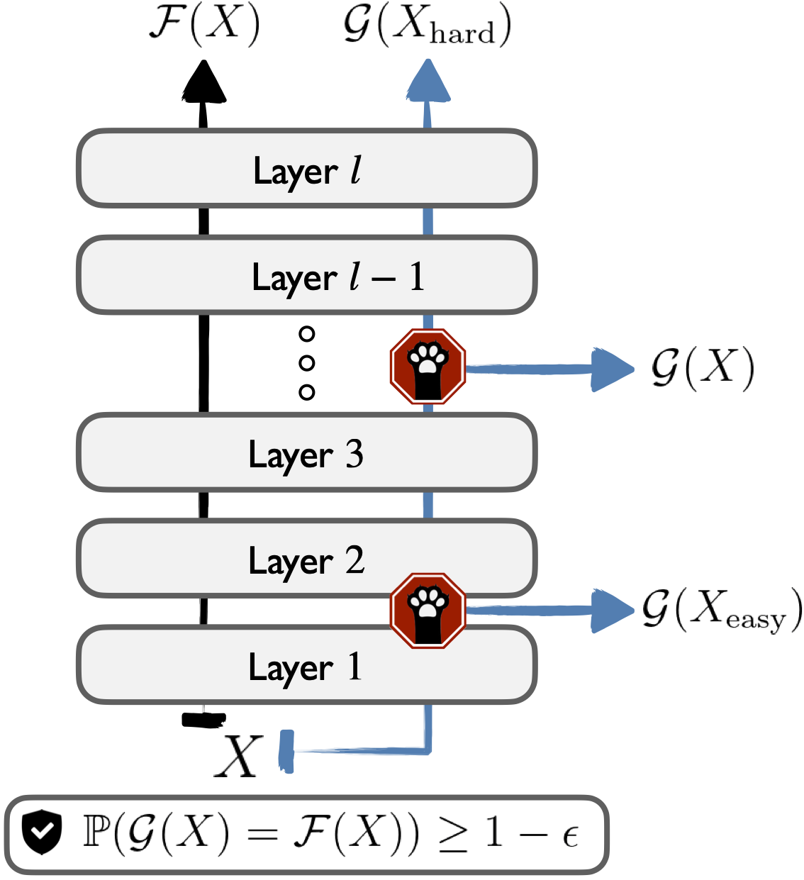
Figure 1: Our CAT model $\mathcal{G}$ can save computational resources by exiting early on certain inputs—while guaranteeing predictive consistency with the full model $\mathcal{F}$.

Figure 2: Confidence levels given by our meta model regarding the consistency of our prediction as computation progresses. Ex.1 from the VitaminC fact verification dataset is “easy”, and is classified consistently by all early classifiers $\mathcal{F}_{k}$ (Supports). The meta confidence captures this, and increases with time. Ex.2 is harder—and the prediction changes ($\texttt{Refutes}/\texttt{NEI}$) as it propagates though the Transformer layers. Appropriately, the meta confidence is low. The exact exit layer of $\mathcal{G}$ is determined as a function of a user-specified tolerance $\epsilon$, see Eq. (1).

Quantifying the uncertainty in a prediction in order to decide when additional computation is needed (or not) is critical to making predictions quickly without excessively sacrificing performance. In this paper, we present Confident Adaptive Transformers (CATs), a general method for increasing Transformer-based model efficiency while remaining confident in the quality of our predictions. Specifically, given a fixed, expensive $l$-layer model $\mathcal{F}(x)$, we create an amortized model $\mathcal{G}(x)$ that includes early classifiers $\{\mathcal{F}_{1},\ldots,\mathcal{F}_{l}\}$. We then make $\mathcal{G}$ provably consistent with the original $\mathcal{F}$ with arbitrarily high probability (e.g., 95% of the time). This process is illustrated in Figure 1.

Our approach builds on conformal prediction (CP), a model-agnostic and distribution-free framework for creating well-calibrated predictions Vovk et al. (2005). Concretely, suppose we have been given $n$ examples, $X_{i}\in\mathcal{X}$, $i=1,\ldots,n$, as unlabeled calibration data, that have been drawn exchangeably from some underlying distribution $P$. Let $X_{n+1}\in\mathcal{X}$ be a new exchangeable test example for which we would like to make a prediction. The aim of our method is to construct $\mathcal{G}$ such that it agrees with $\mathcal{F}$ with distribution-free marginal coverage at a tolerance level $\epsilon\in(0,1)$, i.e.,

$$\mathbb{P}\big{(}\mathcal{G}(X_{n+1})=\mathcal{F}(X_{n+1})\big{)}\geq 1-\epsilon.$$ (1)

We consider $\mathcal{G}$ to be $\epsilon$-consistent if the frequency of error, $\mathcal{G}(X_{n+1})\neq\mathcal{F}(X_{n+1})$, does not exceed $\epsilon$. By design, this ensures that $\mathcal{G}$ preserves at least $(1-\epsilon)$-fraction of $\mathcal{F}$’s original performance. Within these constraints, the remaining challenge is to make $\mathcal{G}$ relatively efficient (e.g., a consistent, but vacuous, model is simply the identity $\mathcal{G}\triangleq\mathcal{F}$).

In order to support an efficient $\mathcal{G}$, we need a reliable signal for inferring whether or not the current prediction is likely to be stable. Past work (e.g., Schwartz et al., 2020) rely on potentially poorly correlated metrics such as the early classifier’s softmax response. We address this challenge by instead directly learning meta “consistency predictors” for each of the $l-1$ early classifiers of our $l$ layer model, by leveraging patterns in past predictions. Figure 2 demonstrates the progression of meta confidence scores across layers when applied to “easy” versus “hard” instances from the VitaminC fact verification task Schuster et al. (2021).

We pair the scores of our meta classifier for each layer with a stopping rule that is calibrated using a unique twist on standard conformal prediction. Traditionally, CP is used to construct prediction sets that cover the desired target (e.g., $Y_{n+1}$) with high probability. We invert the CP problem to first infer the multi-label set of inconsistent layers, and then exit at the first layer that falls in its complement. We then demonstrate that this can be reduced to setting a simple (but well-calibrated) exit threshold for the meta classifier scores. Our resulting algorithm is (1) fast to compute in parallel to the main Transformer, (2) requires only unlabeled data, and (3) is statistically efficient in practice, in the sense that it finds low exit layers on average while still maintaining the required predictive consistency.

We validate our method on four diverse NLP tasks—covering both classification and regression, different label space sizes, and varying amounts of training data. We find that it constitutes a simple-yet-effective approach to confident adaptive prediction with minimal interventions and desirable theoretical guarantees. In short, we provide:

1. A novel theoretical extension of conformal prediction to accommodate adaptive prediction;

2. An effective meta consistency classifier for deriving a confident “early exiting” model;

3. A demonstration of the utility of our framework on both classification and regression tasks, where we show significant efficiency improvements, while guaranteeing high consistency.

2 Related Work

Adaptive computation.

Reducing the computational cost of neural models has received intense interest. Adaptive approaches adjust the amount of computation per example to amortize the total inference cost (see Teerapittayanon et al., 2017; Graves, 2017; Huang et al., 2018; Kaya et al., 2019; Wang et al., 2018, inter alia). As discussed in §1, our method is inspired by the approach of Schwartz et al. (2020) and others Liu et al. (2020); Geng et al. (2021); Zhou et al. (2020), where they preempt computation if the softmax value of any early classifier is above a predefined threshold. Yet unlike our approach, their model is not guaranteed to be accurate. In concurrent work, Xin et al. (2021) propose a meta confidence classifier similar to ours. However, as in previous work, they do not address the calibration part to guarantee consistency.

Confident prediction.

A large amount of research has been dedicated towards calibrating the model posterior, $p_{\theta}(\hat{y}_{n+1}|x_{n+1})$, such that the accuracy, $y_{n+1}=\hat{y}_{n+1}$, is indeed equal to the estimated probability Niculescu-Mizil and Caruana (2005); Gal and Ghahramani (2016); Guo et al. (2017). In theory, these estimates could be leveraged to create confident early exits—e.g., similar to Schwartz et al. (2020). Ensuring calibrated probabilities of this form is hard, however, and existing methods often still suffer from miscalibration. Additionally, many methods exist for bounding the true error of a classifier Langford (2005); Park et al. (2021), but do not give end-users opportunities to control it. More similar to our work, selective classification Geifman and El-Yaniv (2017) allows the model to abstain from answering when not confident, in order to maintain a target error rate only over answered inputs. Our work gives a different and statistically efficient technique applied to consistent prediction.

Conformal prediction.

CP Vovk et al. (2005) typically is formulated in terms of prediction sets $\mathcal{C}(X_{n+1})$, where finite-sample, distribution-free guarantees can be given over the event that $\mathcal{C}$ contains $Y_{n+1}$. As we discuss in §4, internally our method follows a similar approach in which we try to conservatively identify the inadmissible set of all layers that are inconsistent (and exit at the first layer that falls in that set’s complement). Most relevant to our work, Cauchois et al. (2021) presents algorithms for conformal multi-label predictions. We leverage similar methods in our model, but formulate our solution in terms of the complement of a multi-label set of inconsistent predictions. Our work adds to several recent directions that explore CP in the context of risk-mitigating applications (Lei and Candès, 2020; Romano et al., 2020; Bates et al., 2020; Fisch et al., 2021a, inter alia), or meta-learning settings Fisch et al. (2021b).

3 Early Exiting Transformers

In the following, we describe our dynamic early exiting model. We summarize early classification (following previous work) for convenience (§3.1), and then present our novel meta consistency classifier (§3.2). We focus on classification and regression tasks, given a model $\mathcal{F}(x)=y$. We assume that $\mathcal{F}$ maps the input $x\in\mathcal{X}$ into a series of feature representations before making the prediction $y\in\mathcal{Y}$. Here, $\mathcal{F}$ is a multilayered Transformer Vaswani et al. (2017) composed of $l$ layers (although our method can be applied to any multilayer network).

For all downstream tasks we follow standard practice and assume that the input contains a [CLS] token whose representation is used for prediction. For classification, we use a task-specific head, $\mathrm{softmax}(\mathbf{W}_{o}(\phi(\mathbf{W}_{p}\mathbf{h}_{\texttt{[CLS]}})))$, where $\mathbf{h}_{\texttt{[CLS]}}\in\mathbb{R}^{d}$ is the hidden representation of the [CLS] token, $\phi$ is a nonlinear activation, and $\mathbf{W}_{*}$ are linear projections, where $\mathbf{W}_{p}\in\mathbb{R}^{d\times d}$ and $\mathbf{W}_{o}\in\mathbb{R}^{|\mathcal{Y}|\times d}$. Regression is treated similarly, but uses a 1-d output projection, $\mathbf{w}_{o}\cdot\mathbf{h}_{\texttt{[CLS]}}$.

3.1 Early predictors

$\mathcal{F}$’s structure yields a sequence of hidden [CLS] representations, $\{\mathbf{h}^{(1)}_{\texttt{[CLS]}},\ldots,\mathbf{h}^{(l)}_{\texttt{[CLS]}}\}$, where $\mathbf{h}^{(k)}_{\texttt{[CLS]}}\in\mathbb{R}^{d}$ is the representation after applying layer $k$. After each intermediate layer $k<l$, we train an early classification head that is similar to the head used in $\mathcal{F}$, but reduce the dimensionality of the first projection to $\mathbf{W}_{p}^{(k)}\in\mathbb{R}^{d_{e}\times d}$ (this is purely for efficiency). The final $\mathcal{F}_{l}$ is unchanged from $\mathcal{F}$. These extra $(l-1)\times(d_{e}\times d+d_{e}\times|\mathcal{Y}|)$ parameters are quick to tune on top of a fixed $\mathcal{F}$, and we can reuse $\mathcal{F}$’s training data as $\mathcal{D}_{\mathrm{tune}}$. The classifier $\mathcal{F}_{k}(x)=\mathrm{softmax}(\mathbf{W}^{(k)}_{o}(\phi(\mathbf{W}^{(k)}_{p}\mathbf{h}^{(k)}_{\texttt{[CLS]}})))$ is then used after layer $k$ to get an early prediction candidate. Early regression is handled similarly.

3.2 Meta early exit classifier

To decide when to accept the current prediction and stop computation, we require some signal as to how likely it is that $\mathcal{F}_{k}(x)=\mathcal{F}(x)$. Previous work relies on intrinsic measures (e.g., softmax response). Here, we present a meta classifier to explicitly estimate the consistency of an early predictor. Given fixed $\mathcal{F}_{k}$ and $\mathcal{F}$, we train a small binary MLP, $\mathcal{M}_{k}(x)\in\mathbb{R}$, on another unlabeled (limited) sample of task in-domain data, $\mathcal{D}_{\mathrm{meta}}$. As input, we provide the current “early” hidden state $\phi(\mathbf{W}^{(k)}_{p}\mathbf{h}^{(k)}_{\texttt{[CLS]}})$, in addition to several processed meta features, see Table 1. We then train $\mathcal{M}_{k}$ with a binary cross entropy objective, where we maximize the likelihood of predicting $\mathbf{1}\{\mathcal{F}_{k}(x_{i})=\mathcal{F}(x_{i})\}$ for $x_{i}\in\mathcal{D}_{\mathrm{meta}}$.

Using the trained $\mathcal{F}_{k}$ and $\mathcal{M}_{k}$, we define the full adaptive model $\mathcal{G}$ using the prediction rule

where $\bm{\tau}=(\tau_{1},\ldots,\tau_{l-1})$ are confidence thresholds. The key challenge is to calibrate $\tau_{k}$ such that $\mathcal{G}$ guarantees $\epsilon$-consistent performance per Eq. (1).

Meta Feature	Description
$\hat{y}_{k}$	The current prediction.
$\mathrm{history}$	The past $k-1$ predictions, $\hat{y}_{1:k-1}$ (For classification we give $p_{k}(\hat{y}_{k}|x)$).
$p_{k}^{\mathrm{max}}$	Prob. of the prediction, $p_{k}(\hat{y}_{k}|x)$.
$p_{k}^{\mathrm{diff}}$	Difference in prob. of top predictions, $p_{k}(\hat{y}_{k}|x)-{\arg\!\max}_{y_{k}\neq\hat{y}_{k}}~{}p_{k}(y_{k}|x)$.

Table 1: Additional meta features used as input to the meta early exit classifier, $\mathcal{M}_{k}$. Where specified, the probability $p_{k}$ is taken from the model’s early softmax. $p_{k}^{\mathrm{max}}$ and $p_{k}^{\mathrm{diff}}$ are only used for classification tasks.

3.3 Warmup: development set calibration

A simple approach to setting $\bm{\tau}$ is to optimize performance on a development set $\mathcal{D}_{\mathrm{dev}}$, subject to a constraint on the empirical inconsistency:

$$\begin{split}&\bm{\tau}^{*}:=~{}\underset{(\tau_{1},\ldots,\tau_{l-1})}{\mathrm{minimize}}~{}~{}\widehat{\mathbb{E}}_{\mathrm{dev}}[\mathrm{exit}(G(X;\bm{\tau}))]\\ &\text{s.t. }~{}\widehat{\mathbb{E}}_{\mathrm{dev}}[\mathbf{1}\{\mathcal{G}(X;\bm{\tau})=\mathcal{F}(X)\}]\geq 1-\epsilon,\end{split}$$ (3)

where $\mathrm{exit}(\cdot)$ measures the exit layer, and $\widehat{\mathbb{E}}_{\mathrm{dev}}$ is simply the average over $\mathcal{D}_{\mathrm{dev}}$. Using a standard error bound Langford (2005) over a separate split, $\mathcal{D}_{\mathrm{cal}}$, we can then derive the following guarantee:

Proposition 3.1.

Let $X_{i}$, $i=1,\ldots,n$ be an i.i.d. sample with $s=\sum_{i=1}^{n}\mathbf{1}\{\mathcal{G}(X_{i};\bm{\tau})=\mathcal{F}(X_{i})\}$. Then, up to a confidence level $\delta$, we have that

$$\mathbb{P}(\mathbb{P}(\mathcal{G}(X;\bm{\tau})=\mathcal{F}(X))\geq 1-\tilde{\epsilon})\geq 1-\delta,$$ (4)

where $\tilde{\epsilon}$ is the solution to $\mathrm{Beta}(s,n-s+1)=\delta$, and $\mathrm{Beta}$ is the incomplete beta function.

A proof is given in Appendix A. Though in practice $\tilde{\epsilon}$ might be close to $\epsilon$ for most well-behaved distributions, unfortunately Eq. (4) does not give a fully specifiable guarantee as per Eq. (1). Readjusting $\bm{\tau}$ based on $\mathcal{D}_{\mathrm{cal}}$ requires correcting for multiple testing in order to remain theoretically valid, which can quickly become statistically inefficient. In the next section, we provide a novel calibration approach that allows us to guarantee a target performance level with strong statistical efficiency.

4 Conformalized Early Exits

We now formulate the main contribution of this paper, which is a distribution-free and model-agnostic method based on CP for guaranteeing any performance bound an end-user chooses to specify. Our training (§3), conformal calibration (§4), and inference pipelines are summarized in Algorithm 1.

4.1 Conformal formulation

Let $\mathcal{I}(x):=\{i\colon\mathcal{F}_{i}(x)\neq\mathcal{F}(x)\}$ be the index set of layers that are inconsistent with the final model’s prediction. To maintain $\epsilon$-consistency, we must avoid using any of the predictions specified by this set, $\mathcal{F}_{i}(x)$ where $i\in\mathcal{I}(x)$, more than $\epsilon$-fraction of the time for $x\in\mathcal{X}$. In §4.2, we show how $\mathcal{M}_{1:l-1}$ can be paired with a conformal procedure to obtain calibrated thresholds $\bm{\tau}=(\tau_{1},\ldots,\tau_{l-1})$ such that we obtain a conservative prediction of $\mathcal{I}(x)$,

$$\mathcal{C}_{\epsilon}(x):=\{k\colon\mathcal{M}_{k}(x)\leq\tau_{k}\},$$ (5)

where we ensure that $\mathcal{I}(x)\subseteq\mathcal{C}_{\epsilon}(x)$ with probability at least $1-\epsilon$. Proposition 4.1 states our guarantee when $\bm{\tau}$ is paired with $\mathcal{G}$ following Eq. (2).

Proposition 4.1.

Assume that examples $X_{i}$, $i=1,\ldots,n+1$ are exchangeable. For any $\epsilon\in(0,1)$, let the index set $\mathcal{C}_{\epsilon}$ (based on the first $n$ examples) be the output of conformal procedure satisfying

$$\mathbb{P}(\mathcal{I}(X_{n+1})\subseteq\mathcal{C}_{\epsilon}(X_{n+1}))\geq 1-\epsilon.$$ (6)

Define $K:=\min\{j:j\in\mathcal{C}_{\epsilon}^{c}(X_{n+1})\}$, the first exit layer selected by $\mathcal{G}$ following Eq. (2). Then

$$\mathbb{P}(\mathcal{F}_{K}(X_{n+1})=\mathcal{F}(X_{n+1}))\geq 1-\epsilon.$$ (7)

Remark 4.2.

Note that Eq. (6) is stricter than necessary. Fundamentally, we only require that $\mathbb{P}(K\in\mathcal{I}^{c}(X_{n+1}))\geq 1-\epsilon$. Nevertheless, Eq. (6) is easier to calibrate, and leads to strong empirical results despite being theoretically conservative.

Remark 4.3.

During inference we do not fully construct $\mathcal{C}_{\epsilon}$; it is only used to calibrate $\bm{\tau}$ beforehand.

4.2 Conformal calibration

We now describe our conformal procedures for calibrating $\bm{\tau}$. Conformal prediction is based on hypothesis testing, where for a given input $x$ and possible output $y$, a statistical test is performed to accept or reject the null hypothesis that the pairing $(x,y)$ is correct. In our setting, we consider the null hypothesis that layer $k$ is inconsistent, and we use $\mathcal{M}_{k}(x)$ as our test statistic. Since $\mathcal{M}_{k}$ is trained to predict $\mathbf{1}\{\mathcal{F}_{k}(x_{i})=\mathcal{F}(x_{i})\}$, a high value of $\mathcal{M}_{k}(x)$ indicates how “surprised” we would be if layer $k$ was in fact inconsistent with layer $l$ for input $x$. Informally, a low level of surprise indicates that the current input “conforms” to past data. To rigorously quantify the degree of conformity via the threshold $\tau_{k}$ for predictor $\mathcal{M}_{k}$, we use a held-out set of $n$ unlabeled, exchangeable examples, $\mathcal{D}_{\mathrm{cal}}$.

4.2.1 Independent calibration

As a first approach, we construct $\mathcal{C}_{\epsilon}(x)$ by composing $l-1$ separate tests for $\mathcal{F}_{k}(x)\neq\mathcal{F}(x)$, each with significance $\alpha_{k}$, where $\alpha_{k}$ are corrected for multiple testing. Let $v_{k}^{(1:n,\infty)}$ denote the inflated empirical distribution of inconsistent layer scores,

$$\{\mathcal{M}_{k}(x_{i})\colon x_{i}\in\mathcal{D}_{\mathrm{cal}},\mathcal{F}_{k}(x_{i})\neq\mathcal{F}(x_{i})\}\cup\{\infty\}.$$

Inflating the empirical distribution is critical to our finite sample guarantee, see Appendix A. We then define $\tau^{\mathrm{ind}}_{k}=\mathrm{Quantile}\big{(}1-\alpha_{k},v_{k}^{(1:n,\infty)}\big{)}$, and predict the inconsistent index set at $x\in\mathcal{X}$ as

$$\mathcal{C}_{\epsilon}^{\mathrm{ind}}(x)=\left\{k\colon\mathcal{M}_{k}(x)\leq\tau_{k}^{\mathrm{ind}}\right\}.$$ (8)

The following theorem states how to set each $\alpha_{k}$ such that the quantiles $\tau_{k}^{\mathrm{ind}}$ yield a valid $\mathcal{C}_{\epsilon}^{\mathrm{ind}}$.

Theorem 4.4.

Let $\alpha_{k}=\omega_{k}\cdot\epsilon$, where $\omega_{k}$ is a weighted Bonferroni correction, i.e., $\sum_{k=1}^{l-1}\omega_{k}=1$. Then $\mathcal{C}_{\epsilon}^{\mathrm{ind}}(X_{n+1})$ is a valid set that satisfies Eq. (6).

Remark 4.5.

$\omega_{1:l-1}$ can be tuned on a development set $\mathcal{D}_{\mathrm{dev}}$ as long as $\mathcal{D}_{\mathrm{dev}}$ is distinct from $\mathcal{D}_{\mathrm{cal}}$.

Algorithm 1 Consistent accelerated inference.

Definitions: $\mathcal{F}$ is a multilayered classifier trained on $\mathcal{D}_{\mathrm{train}}$. $\mathcal{D}_{\mathrm{tune}}$, $\mathcal{D}_{\mathrm{meta}}$ and $\mathcal{D}_{\mathrm{scale}}$ are collections of in-domain unlabeled data points (in practice, we reuse $\mathcal{D}_{\mathrm{train}}$ and divide it to 70/20/10%, respectively). $\mathcal{D}_{\mathrm{cal}}$ has in-domain unlabeled examples not in $\mathcal{D}_{\mathrm{train}}$ (In practice, we take a subset of the task’s validation set). $\epsilon$ is the user-specified consistency tolerance.

1:function Train ($\mathcal{F}$, $\mathcal{D}_{\mathrm{tune}}$, $\mathcal{D}_{\mathrm{meta}}$)

2:   # Learns $\mathcal{F}_{{1}\dots l-1}$ and $\mathcal{M}_{{1}\dots l-1}$ components

3:   # of amortized model $\mathcal{G}$ for Eq. (2) (see §3.1 and §3.2).

4:   Initialize $\mathcal{G}$ from $\mathcal{F}$ and add early prediction heads.

5:   # (All of $\mathcal{F}$’s base parameters in $\mathcal{G}$ are frozen.)

6:   Train prediction heads $\mathcal{F}_{{1}\dots l-1}$ on $\mathcal{D}_{\mathrm{tune}}$.

7:   Add meta early exit classifiers $\mathcal{M}_{{1}\dots l-1}$ to $\mathcal{G}$.

8:   # (All of $\mathcal{G}$’s other parameters are frozen.)

9:   Train meta early exit classifiers $\mathcal{M}_{{1}\dots l-1}$ on $\mathcal{D}_{\mathrm{meta}}$.

10:   Optionally apply temperature scaling using $\mathcal{D}_{\mathrm{scale}}$.

11:   return $\mathcal{G}$

12:function Calibrate ($\mathcal{G}$, $\mathcal{D}_{\mathrm{cal}}$, $\epsilon$)

13:   # Sets thresholds $\bm{\tau}$ of amortized model $\mathcal{G}$ for Eq. (2)

14:   # using shared calibration (see §4.2.2).

15:   $M$ $\leftarrow$ $\{\infty\}$

16:   for $x\in\mathcal{D}_{\mathrm{cal}}$ do

17:      $S$ $\leftarrow$ $\{\}$

18:      # Record all inconsistent layers for input $x$.

19:      # Keep the highest (false) confidence score.

20:      for $k\in[1,l-1]$ do

21:         if $\mathcal{F}_{k}(x)\neq\mathcal{F}(x)$ then

22:            $S$ $\leftarrow$ $S\cup\mathcal{M}_{k}(x)$                

23:      $M$ $\leftarrow$ $M\cup\max{(S)}$    

24:   # Share one threshold across layers.

25:   $\tau^{\mathrm{share}}$ $\leftarrow$ $\mathrm{Quantile}\big{(}1-\epsilon,M\big{)}$

26:   return $[\tau^{\mathrm{share}}]\times(l-1)$

27:function Predict ($\mathcal{G},\bm{\tau}$, $x$)

28:   # Implements Eq. (2) to exit early with confidence.

29:   for $k\in[1,l-1]$ do

30:      Compute the $k$-th prediction head of $\mathcal{G}$, $\mathcal{F}_{k}(x)$.

31:      if $\mathcal{M}_{k}(x)>\tau_{k}$ then

32:         return $\mathcal{F}_{k}(x)$          

33:   # Fallback to prediction using full computation.

34:   return $\mathcal{F}_{l}(x)$

4.2.2 Shared calibration

$\mathcal{C}_{\epsilon}^{\mathrm{ind}}$ has the advantage of calibrating each layer independently. As $l$ grows, however, $\alpha_{k}$ will tend to $0$ in order to retain validity (as specified by Theorem 4.4). As a result, $\mathcal{C}_{\epsilon}^{\mathrm{ind}}$ will lose statistical efficiency. Following a similar approach to Cauchois et al. (2021) and Fisch et al. (2021a), we compute a new test statistic, $\mathcal{M}_{\mathrm{max}}$, as

We discard ill-defined values when $\mathcal{M}_{\mathrm{max}}(x)=\max\varnothing$. $\mathcal{M}_{\mathrm{max}}(x)$ reflects the worst-case confidence across inconsistent layers for input $x$ (i.e., where $\mathcal{M}_{k}(x)$ predicts a high consistency likelihood for layer $k$ when layer $k$ is, in fact, inconsistent). This worst-case statistic allows us to keep a constant significance level $\epsilon$, even as $l$ grows. Let $m^{(1:n,\infty)}$ denote the inflated empirical distribution,

We then define a single threshold shared across layers, $\tau^{\mathrm{share}}=\mathrm{Quantile}\big{(}1-\epsilon,m^{(1:n,\infty)}\big{)}$, and predict the inconsistent index set at $x\in\mathcal{X}$ as

$$\mathcal{C}_{\epsilon}^{\mathrm{share}}(x)=\left\{k\colon\mathcal{M}_{k}(x)\leq\tau^{\mathrm{share}}\right\}$$ (10)

Theorem 4.6.

For any number of layers $l\in\mathbb{N}^{+}$, $\mathcal{C}_{\epsilon}^{\mathrm{share}}(X_{n+1})$ is a valid set that satisfies Eq. (6).

5 Experimental Setup

For our main results, we use an Albert-xlarge model (Lan et al., 2020) with 24 Transformer layers. Results using an Albert-base model and a RoBERTa-large model (Liu et al., 2019) are in Appendix C. See Appendix B for implementation details. We did not search across different values for the hyper-parameters of $\mathcal{F}$ or $\mathcal{G}$ as our approach is general and guarantees consistency for any $\mathcal{F}$ with any nonconformity measure (See Appendix C.2). Tuning the hyper-parameters could further improve the efficiency of $\mathcal{G}$ while preserving consistency.

5.1 Tasks

We evaluate our methods on three classification tasks with varying label space size $|\mathcal{Y}|$ and difficulty: IMDB (Maas et al., 2011) sentiment analysis on movie reviews, VitaminC (Schuster et al., 2021) fact verification with Wikipedia articles, and AG (Gulli, 2004; Zhang et al., 2015) news topic classification. We also evaluate on the STS-B (Cer et al., 2017) semantic textual similarity regression task where $\mathcal{Y}\in[0,5]\subset\mathbb{R}$. Dataset statistics, along with the test set performance of our original $\mathcal{F}$ model (Albert-xlarge), are contained in Table 2.

Dataset	$|\mathcal{Y}|$	Train	Dev.	Test	$\mathcal{F}$ test perf.
IMDB	2	20K	5K	25K	94.0
VitaminC	3	370K	10K∗	55K	90.6
AG News	4	115K	5K	7.6K	94.4
STS-B	$\infty$	5.7K	1.5K	1.4K	89.8

Table 2: Task dataset and label space sizes. The rightmost column reports either test accuracy (classification) or Pearson-correlation (regression). ^∗We downsample the 63K public development set to expedite validation.

5.2 Baselines

In addition to our main methods discussed in §4.2, we compare to several non-CP baselines. Note that the following methods are not guaranteed to give well-calibrated performance (as our CP ones are).

Static.

We use the same number of layers for all inputs. We choose the exit layer as the first one that obtains the desired consistency on average on $\mathcal{D}_{\text{cal}}$.

Softmax threshold.

Following Schwartz et al. (2020), we exit on the first layer where $p_{k}^{\mathrm{max}}\geq 1-\epsilon$, where $p_{k}^{\mathrm{max}}$ denotes the maximum softmax response of our early classifier. Softmax values are calibrated using temperature scaling Guo (2017) on another held-out (labeled) data split, $\mathcal{D}_{\mathrm{scale}}$.

Meta threshold.

Even if perfectly calibrated, $p_{k}^{\mathrm{max}}$ from softmax thresholding is not measuring consistency likelihood $\mathbb{P}(\mathcal{G}(X)=\mathcal{F}(X)\mid X=x)$, but rather $\mathbb{P}(\mathcal{G}(X)=Y\mid X=x)$. This is equivalent if $\mathcal{F}$ is an oracle, but breaks down when $\mathcal{F}$ is not. We also experiment with thresholding the confidence value of our meta classifier (§3.2) in a similar way (i.e., exiting when it exceeds $1-\epsilon$).

5.3 Evaluation

For each task, we use a proper training, validation, and test set. We use the training set to learn $\mathcal{F}$ and $\mathcal{G}$. We perform model selection on the validation set, and report final numbers on the test set. For all methods, we report the marginalized results over 25 random trials, where in each trial we partition the data into 80% $\mathcal{D}_{\mathrm{cal}}$ ($x_{1:n}$) and 20% $\mathcal{D}_{\mathrm{test}}$ ($x_{n+1}$). In order to compare different methods across all tolerance levels, we plot each metric as a function of $\epsilon$. Shaded regions show the $16$-$84$th percentiles across trials. We report the following metrics:

Consistency.

We measure the percent of inputs for which the prediction of the CAT model $\mathcal{G}$ is the same as the full Transformer on our test prediction, i.e., $\mathcal{G}(X_{n+1})=\mathcal{F}(X_{n+1})$. For regression tasks, we count a prediction as consistent if it is within a small margin $\tau$ from the reference (we use $\tau=0.5$). As discussed in $\S\ref{sec:introduction}$, if $\mathcal{G}$ is $\epsilon$-consistent, we can also derive an average performance lower bound: it will be at least $(1-\epsilon)\times\mathcal{F}$’s average performance.

Layers ($\mathbf{\shortdownarrow}$).

We report the computational cost of the model as the average number of Transformer layers used. Our goal is to improve the efficiency (i.e., use fewer layers) while preserving $\epsilon$-consistency. We choose this metric over absolute run-time to allow for implementation-invariant comparisons, but we provide a reference analysis next, to permit easy approximate conversions.

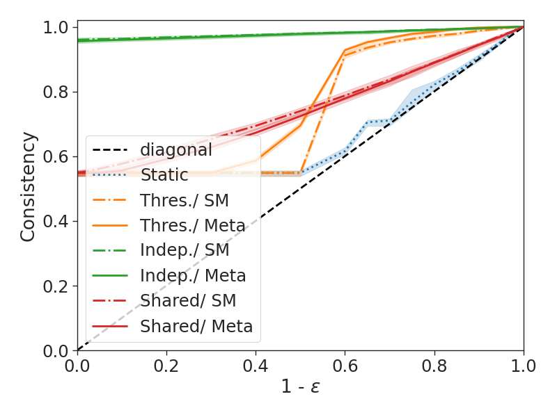
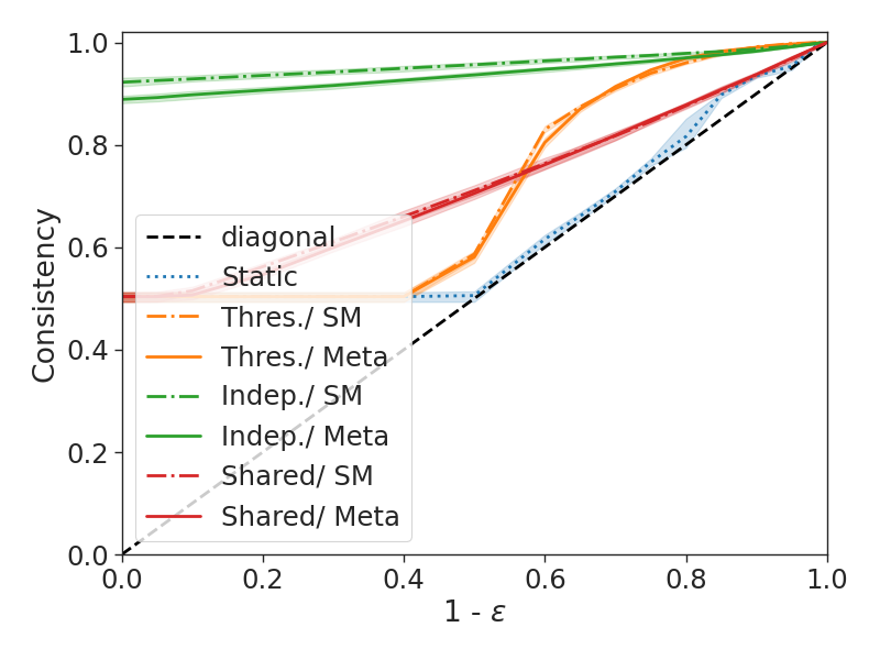
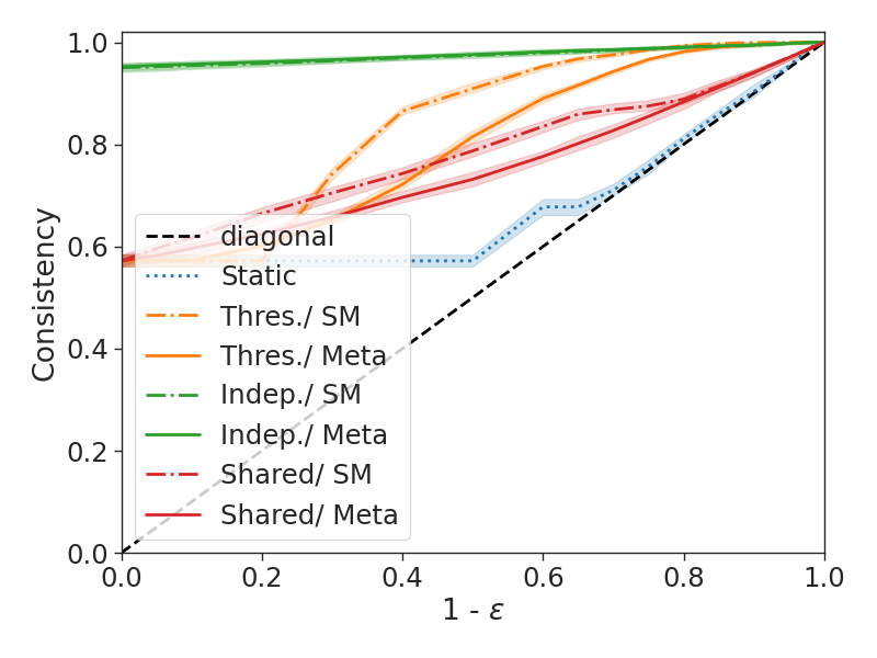
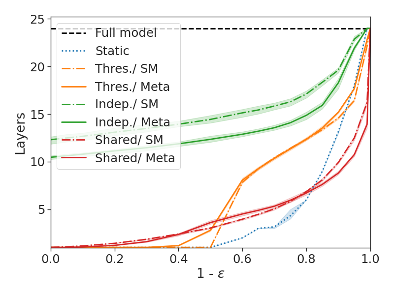
(a) IMDB

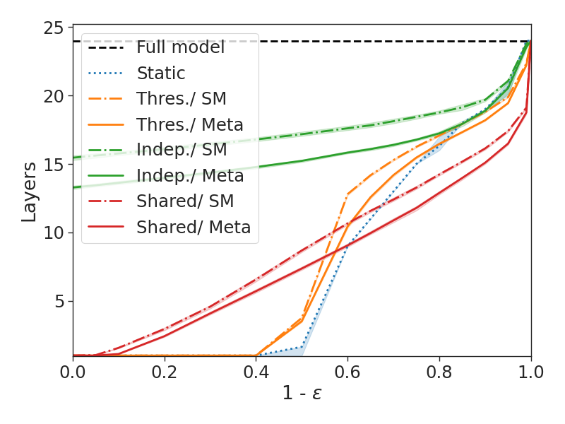
(b) VitaminC

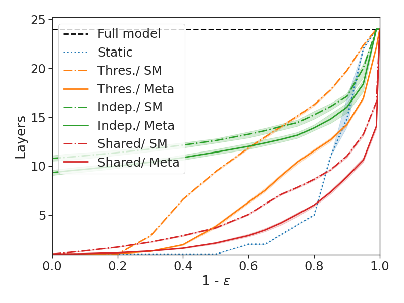
(c) AG News

Figure 3: Classification results (dev). While both our CP-based methods give valid consistencies (above diagonal), shared calibration generally results in earlier exits. This advantage is especially pronounced at smaller tolerance levels (right-hand side), where it significantly outperforms other approaches. Our meta-learned confidence measure $\mathcal{M}_{k}$ improves over using the softmax response as a drop-in replacement, especially for tasks with larger $|\mathcal{Y}|$. Note that we care more about the right-hand side behavior, (i.e., larger $1-\epsilon$), as it corresponds to higher consistency.

5.4 Absolute runtime analysis

The exact run-time of $\mathcal{G}$ depends on the efficiency of the hardware, software, and implementation used. Ideally, the early and meta classifiers can run in parallel with the following Transformer layer (layer $k+1$). As long as they are faster to compute concurrently than a single layer, this will avoid incurring any additional time cost. An alternative naive synchronous implementation could lead to inefficiencies when using a small tolerance $\epsilon$.

We provide a reference timing for the IMDB task implemented with the Transformers (Wolf et al., 2020) library, PyTorch 1.8.1 (Paszke et al., 2019), and an A100-PCIE-40GB Nvidia GPU with CUDA 11.2. A full forward path of an Albert-xlarge takes $22.32$ms per input, $0.85$ms $\times 24$ for the transformer layers and $1.95$ms for the embedding layer and top classifier. Our early classifier takes $0.20$ms and the meta classifier takes $0.11$ms. Therefore, with a naive implementation, a CAT model $\mathcal{G}$ with an average exit layer less than $17.6$ with the meta classifier, or $19.5$ without, will realize an overall reduction in wall-clock time relative to the full $\mathcal{F}$.

We report example speedup times with the naive implementation in §6.3, as well as an implementation invariant multiply-accumulate operation (MACs) reduction measure. The added computational effort per layer of the early predictor and meta-classifier is marginal (only $66,304$ and $1,920$ MACs, respectively). In comparison, Albert-xlarge with an input length of 256 has $\sim 3\cdot 10^{11}$ MACs.

6 Experimental Results

We present our main results. We experiment with both our meta classifier $\mathcal{M}_{k}$ confidence score (Meta, §3.2), and, for classification tasks, the early classifier’s softmax response, $p_{k}^{\mathrm{max}}$ (SM), as a drop-in replacement for $\mathcal{M}_{k}$ (at no additional computational cost). Appendix C reports results with other drop-in $\mathcal{M}_{k}$ replacements, in addition to results using our naive development set calibration approach (§3.3). Appendix D provides qualitative examples.

6.1 Classification results

Method	IMDB			VitaminC			AG News
	Consist.	Acc.	Layers	Consist.	Acc.	Layers	Consist.	Acc.	Layers
$\underline{1-\epsilon=0.95}$:		$(88.50)$			$(86.10)$			$(89.02)$
Static	$95.54$	$92.88$	$18.36$	$95.51$	$89.40$	$21.00$	$95.48$	$93.20$	$22.00$
Thres./ SM	$99.65$	$94.01$	$16.55$	$99.83$	$90.59$	$20.07$	$100.00$	$94.44$	$22.28$
Thres./ Meta	$99.98$	$93.96$	$17.73$	$99.73$	$90.59$	$19.67$	$99.41$	$94.00$	$16.21$
Indep./ Meta	$99.66$	$93.82$	$15.69$	$99.07$	$89.97$	$19.60$	$99.81$	$94.31$	$20.58$
Shared/ SM	$97.17$	$93.24$	$12.65$	$96.87$	$88.99$	$17.58$	$97.15$	$93.43$	$13.24$
Shared/ Meta	$97.15$	$92.71$	$\mathbf{10}.\mathbf{83}$	$96.91$	$89.01$	$\mathbf{16}.\mathbf{79}$	$97.08$	$92.50$	$\mathbf{10}.\mathbf{17}$
$\underline{1-\epsilon=0.90}$:		$(83.84)$			$(81.57)$			$(84.33)$
Static	$90.82$	$89.47$	$14.00$	$92.57$	$87.80$	$19.00$	$90.88$	$89.10$	$14.00$
Thres./ SM	$98.88$	$93.93$	$14.71$	$99.05$	$90.27$	$18.91$	$99.68$	$94.21$	$19.53$
Thres./ Meta	$99.75$	$93.86$	$15.30$	$99.10$	$90.31$	$18.45$	$98.90$	$93.82$	$13.50$
Indep./ Meta	$99.39$	$93.67$	$14.85$	$98.29$	$89.42$	$18.50$	$99.60$	$94.18$	$17.65$
Shared/ SM	$94.34$	$91.77$	$10.30$	$93.73$	$87.00$	$16.40$	$94.50$	$92.01$	$10.79$
Shared/ Meta	$94.36$	$90.78$	$\mathbf{9}.\mathbf{01}$	$93.83$	$86.89$	$\mathbf{15}.\mathbf{33}$	$94.29$	$90.26$	$\mathbf{8}.\mathbf{35}$

Table 3: Classification results (test) for specific tolerance levels. We report the accuracy lower bound guaranteed by our CP methods in parentheses. Shared/ Meta is reliably the most efficient method (and is $\epsilon$-consistent). Greyed rows reflect approaches without guarantees; our CAT approaches with guarantees are presented below them.

Figure 3 summarizes the average consistency and number of layers used by $\mathcal{G}$ as a function of $\epsilon$, while Table 3 presents results for specific $\epsilon$ on task test sets. Independent calibration proves to be quite conservative due to the loss of statistical power from the loose union bound of the Bonferroni correction for large $l$ (here $l=24$). At some levels of $\epsilon$, non-CP baselines perform competitively, however, they lack formal guarantees. Overall, for the most critical tolerance levels (small $\epsilon$, right-hand side of the plots), our shared method leads to significant efficiency gains while still maintaining the desired level of consistency (above the diagonal).

The effectiveness of our meta predictor, $\mathcal{M}_{k}$, is most pronounced for tasks with $|\mathcal{Y}|>2$, where the drop-in softmax score (SM) becomes less indicative of consistency. Both SM and Meta are relatively well-calibrated for IMDB and VitaminC, which makes the threshold-based exit rule a competitive baseline. Still, our Shared/ Meta method provides both reliable and significant gains.

The computational advantage of our CAT model is dependent on the average difficulty of the task and the implementation. As Table 3 shows, allowing up to an $\epsilon$ of 10% inconsistency, for two of the tasks we cut down the average Transformer layer to only $9$ out of $24$ using our Shared/ Meta model. This leads to an approximate speedup of $1.8\times$ with a synchronous implementation and of $2.7\times$ with a concurrent one, compared to running the full model. Moreover, Figure 5 illustrates the user’s control over available computational resources via modulating $\epsilon$. Decreasing $\epsilon$ increases the confidence level required before committing to the early classifier’s prediction (thereby increasing the average number of required layers), and vice-versa.

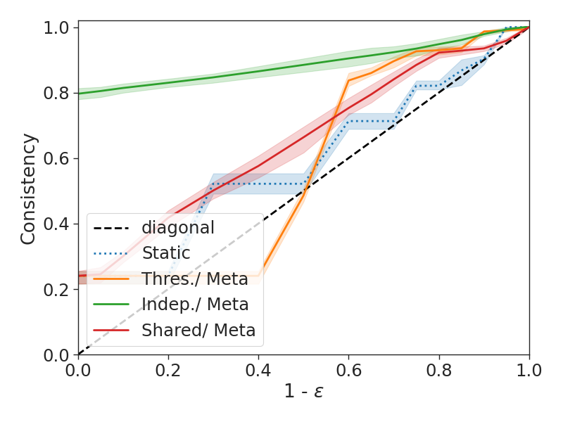
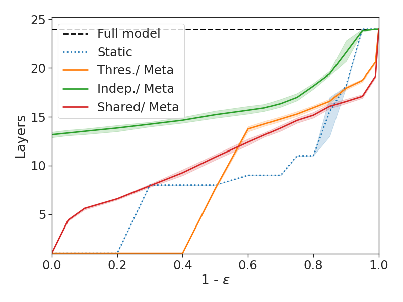
Figure 4: Dev results for the STS-B regression task.

6.2 Regression results

Table 4 and Figure 4 present results for our regression task, where we see similar trends. Here, an attractive advantage of our meta confidence predictor is its generalizability to multiple task output types. Notice that the event space of $\mathbf{1}\{\mathcal{G}(X)=\mathcal{F}(X)\}=\{0,1\}$ always, regardless of the original $\mathcal{Y}$. This allows it to be easily adapted to tasks beyond classification, such as regression, where traditional softmax-based confidence measures (as used in, e.g., Schwartz et al. (2020)) are absent.

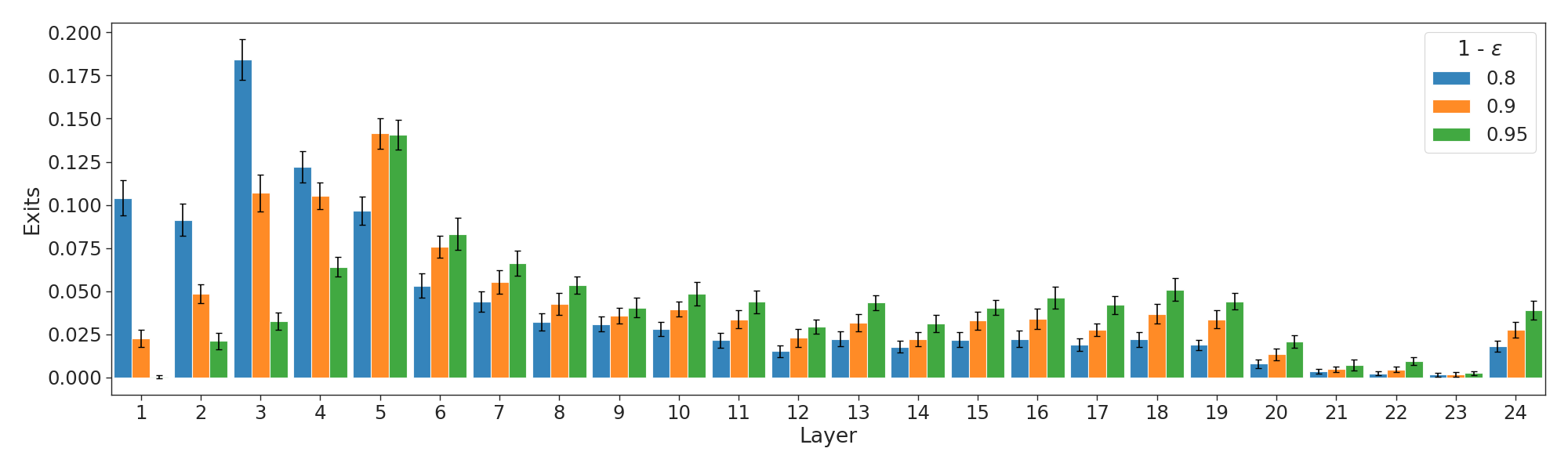
Figure 5: Distribution of exit layers per tolerance level $\epsilon$ for the IMDB task (dev set) with Shared/ Meta. Larger $\epsilon$ allows the CAT model to shift its predictions earlier by permitting for more inconsistencies with the full model $\mathcal{F}$.

Method	Consist.	Layers
$\underline{1-\epsilon=0.95}$:
Static	$100.00$	$24.00$
Thres./ Meta	$99.87$	$19.19$
Indep./ Meta	$99.29$	$23.60$
Shared/ Meta	$96.42$	$\mathbf{17}.\mathbf{64}$
$\underline{1-\epsilon=0.90}$:
Static	$92.51$	$20.00$
Thres./ Meta	$99.19$	$18.53$
Indep./ Meta	$97.77$	$20.26$
Shared/ Meta	$92.65$	$\mathbf{17}.\mathbf{29}$

Table 4: Test results for the STS-B regression task.

Method	Amortized time ($100\cdot T_{\mathcal{G}}/T_{\mathcal{F}}$)				MACs reduction ($|\mathcal{F}|/|\mathcal{G}|$)
	IMDB	VitaminC	AG News	STS-B	IMDB	VitaminC	AG News	STS-B
Thres./ SM	$76.91$	$96.66$	$99.58$	N/A	$1.63$	$1.27$	$1.23$	N/A
Thres./ Meta	$87.22$	$103.59$	$77.87$	$104.01$	$1.57$	$1.30$	$1.78$	$1.30$
Indep./ Meta	$84.88$	$103.85$	$99.44$	$113.00$	$1.62$	$1.30$	$1.36$	$1.18$
Shared/ SM	$56.16$	$\textbf{84}.\textbf{86}$	$58.47$	N/A	$2.33$	$1.46$	$2.22$	N/A
Shared/ Meta	$\textbf{54}.\textbf{53}\ \%$	$87.38\ \%$	$\textbf{51}.\textbf{10}\ \%$	$\textbf{97}.\textbf{56}\ \%$	$\times\textbf{2}.\textbf{66}$	$\times\textbf{1}.\textbf{57}$	$\times\textbf{2}.\textbf{87}$	$\times\textbf{1}.\textbf{39}$

Table 5: Reference time speedup and model complexity reduction for $1-\epsilon=0.90$ (see Table C.2 for 0.95). We compute the amortized time with the naive synchronous implementation (§5.4). A more efficient implementation can further reduce the time of $\mathcal{G}$. The MACs reduction measure is implementation agnostic and expresses the ratio of computational effort saved by $\mathcal{G}$. Our CAT models (non-greyed lines) not only guarantee $1-\epsilon$ consistency with $\mathcal{F}$, but are also significantly more efficient in practice when using Shared calibration.

6.3 Example efficiency gains

Following the analysis in §5.4, we compute the amortized inference time with a naive implementation and report its percentage out of the full model. As Table 5 shows, our Shared calibration is the most efficient method on all four tasks. For tasks with many easy inputs (IMDB and AG News), our Shared/ Meta method can save $45\%$ - $49\%$ of the inference time when $1-\epsilon=0.90$. Unsurprisingly, the absolute speedup is less significant for harder tasks, but increases with higher tolerance levels.

On VitaminC, even though the Meta measure allows exiting on earlier layers, its additional meta classifiers result in slightly slower inference on average at this tolerance level, compared to our Shared/ SM. With a more efficient concurrent implementation, the Meta measure will be favorable.

We also compute the MACs reduction metric which is independent of the specific implementation or hardware and shows the number of multiply-accumulate operations of the full model compared to our CAT model. As demonstrated in Table 5, our Shared/ Meta method is most effective in reducing the computational effort across all tasks for the two examined tolerance levels.

7 Conclusion

The ability to make predictions quickly without excessively degrading performance is critical to production-level machine learning systems. In fact, being capable of quantifying the uncertainty in a prediction and deciding when additional computation is needed (or not) is a key challenge for any intelligent system (e.g., see the System 1 vs. System 2 dichotomy explored in Kahneman (2011)).

In this work, we addressed the crucial challenge of deciding when to sufficiently trust an early prediction of Transformer-based models by learning from their past predictions. Our Confident Adaptive Transformers (CATs) framework leverages meta predictors to accurately assess whether or not the prediction of a simple, early classifier trained on an intermediate Transformer representation is likely to already be consistent with that of the full model $\mathcal{F}(X)$ (i.e., after all $l$ layers of $\mathcal{F}$ are computed). Importantly, we develop a new conformal prediction approach for calibrating the confidence of the meta classifier that is (1) simple to implement, (2) fast to compute alongside the Transformer, (3) requires only unlabeled data, and (4) provides statistically efficient marginal guarantees on the event that the prediction of the faster, amortized CAT model is consistent with that of the full $\mathcal{F}$. Our results on multiple tasks demonstrate the generality of our approach, and its effectiveness in consistently improving computational efficiency—all while maintaining a reliable margin of error.

Appendix A Proofs

We first state the following useful lemma on inflated sample quantiles.

Lemma A.1.

Let $\mathrm{Quantile}(\alpha;F)$ denote the $\alpha$ quantile of distribution $F$. Let $V_{1:n}$ denote the empirical distribution over random variables $\{V_{1},\ldots,V_{n}\}$. Furthermore, assume that $V_{i}$, $i=1,$ $\ldots,n+1$ are exchangeable. Then for any $\alpha\in(0,1)$, we have $\mathbb{P}\left(V_{n+1}\leq\mathrm{Quantile}(\alpha,V_{1:n}\cup\{\infty\})\right)\geq\alpha.$

Proof.

This is a well-known result. Given support points $v_{1},\ldots,v_{n}\in\mathbb{R}$ for a discrete distribution $F$, let $q=\mathrm{Quantile}(\alpha;F)$. Any points $v_{i}>q$ do not affect this quantile, i.e., if we consider a new distribution $\tilde{F}$ where all points $v_{i}>q$ are mapped to arbitrary values also larger than $q$ then $\mathrm{Quantile}(\alpha;F)=\mathrm{Quantile}(\alpha;\tilde{F})$. Accordingly, for the exchangeable $V_{i}$, we have

$$V_{n+1} >\mathrm{Quantile}(\alpha;V_{1:n}\cup\{\infty\})\Longleftrightarrow$$

$$V_{n+1}>\mathrm{Quantile}(\alpha;V_{1:(n+1)}).$$

Equivalently, we also have that

$$V_{n+1} \leq\mathrm{Quantile}(\alpha;V_{1:n}\cup\{\infty\})\Longleftrightarrow$$

$$V_{n+1}\leq\mathrm{Quantile}(\alpha;V_{1:(n+1)}).$$

Given the discrete distribution over the $n+1$ variables $V_{i}$, $V_{n+1}\leq\mathrm{Quantile}(\alpha;V_{1:(n+1)})$ implies that $V_{n+1}$ is among the $\lceil\alpha(n+1)\rceil$ smallest of $V_{1:(n+1)}$. By exchangeability, this event occurs with probability at least $\frac{\lceil\alpha(n+1)\rceil}{n+1}\geq\alpha$. ∎

A.1 Proof of Proposition 3.1

Proof.

This result is based on Clopper-Pearson confidence interval for Binomial random variables Clopper and Pearson (1934). As the binary events $\mathbf{1}\{\mathcal{G}(X_{i};\bm{\tau})=\mathcal{F}(X_{i})\}$ are i.i.d., the sum $s$ is Binomial. Directly applying a one-sided Clopper-Pearson lower bound on the true success rate, $\mathbb{P}(\mathcal{G}(X_{i};\bm{\tau})=\mathcal{F}(X_{i}))$, gives the result. ∎

A.2 Proof of Proposition 4.1

Proof.

We prove by simple calculation using the property assumed in Eq. (6).

$$\mathbb{P}(\mathcal{F}_{K}( X_{n+1})=\mathcal{F}(X_{n+1}))$$

$$=\mathbb{P}(\min\mathcal{C}_{\epsilon}^{c}(X_{n+1})\in\mathcal{I}^{c}(X_{n+1}))$$

$$\geq\mathbb{P}(\mathcal{C}_{\epsilon}^{c}(X_{n+1})\subseteq\mathcal{I}^{c}(X_{n+1}))$$

$$=\mathbb{P}(\mathcal{I}(X_{n+1})\subseteq\mathcal{C}_{\epsilon}(X_{n+1}))$$

$$\geq 1-\epsilon.$$

∎

A.3 Proof of Theorem 4.4

Proof.

For a given $k$, let $V_{k}^{(i)}:=\mathcal{M}_{k}(X_{i})$ denote the random meta confidence values used for calibration, and $V_{k}^{(n+1)}:=\mathcal{M}_{k}(X_{n+1})$ the random test point. For all $k$, $\mathcal{M}_{k}$ is trained and evaluated on separate data ($\mathcal{D}_{\mathrm{meta}}$ vs $\mathcal{D}_{\mathrm{cal}}\cup\mathcal{D}_{\mathrm{test}}$), preserving exchangeability. Therefore, as $X_{1:n+1}$ are exchangeable, then $V_{k}^{(1:n+1)}$ are also exchangeable.

Layer $k$ is included in $\mathcal{C}_{\epsilon}^{\mathrm{ind}}$ iff $V_{k}^{(n+1)}\leq\mathrm{Quantile}(1-\alpha_{k},V_{k}^{(1:n)}\cup\{\infty\})$. For a given $k$, this happens with probability at least $1-\alpha_{k}$ by Lemma A.1. Taken over all $k\in\mathcal{I}(X_{n+1})$ where $|\mathcal{I}(X_{n+1})|$ is at most $l-1$ (i.e., all early layers are inconsistent), we have

$$\mathbb{P}(\mathcal{I}( X_{n+1})\subseteq\mathcal{C}_{\epsilon}^{\mathrm{ind}}(X_{n+1}))$$

$$=1-\mathbb{P}\Big{(}\bigcup_{k\in\mathcal{I}}\{k\not\in\mathcal{C}_{\epsilon}^{\mathrm{ind}}(X_{n+1})\}\Big{)}$$

$$\geq 1-\sum_{k\in\mathcal{I}}\mathbb{P}(k\not\in\mathcal{C}_{\epsilon}^{\mathrm{ind}}(X_{n+1})$$

$$=1-\sum_{k\in\mathcal{I}}\alpha_{k}$$

$$\geq 1-\epsilon.$$

The last inequality is given by the Bonferroni constraint, i.e., $\alpha_{k}=\omega_{k}\cdot\epsilon$, where $\sum_{i=1}^{l-1}\omega_{i}=1$ ∎

A.4 Proof of Theorem 4.6

Proof.

By the same argument as Theorem 4.4, the meta scores $\mathcal{M}_{k}(X_{i})$ are exchangeable. Since $\mathcal{M}_{\mathrm{max}}$ operates symmetrically across all $X_{i}$, $M^{(i)}=\mathcal{M}_{\mathrm{max}}(X_{i})$ are also exchangeable.

Let $M^{(n+1)}$ denote the maximum meta score across inconsistent layers for the new test point. By Lemma A.1, this falls below $\mathrm{Quantile}(1-\epsilon,M^{(1:n)}\cup\{\infty\})$ with probability at least $1-\epsilon$. Since $M^{(n+1)}$ reflects the maximum meta score, this entails that the meta scores of all other inconsistent layers $k\in\mathcal{I}(X_{n+1})$ for $X_{n+1}$ will be below $\mathrm{Quantile}(1-\epsilon,M^{(1:n)}\cup\{\infty\})$ if $M^{(n+1)}$ is, and thereby be included in $\mathcal{C}_{\epsilon}^{\mathrm{share}}(X_{n+1})$. This gives the bound in Eq. (6). ∎

Nonconformity	IMDB			VitaminC			AG News
measure	Consist.	Bound	Layers	Consist.	Bound	Layers	Consist.	Bound	Layers
$\underline{1-\epsilon=0.95}$:
SM	$95.16$	$93.74$	$10.39$	$94.84$	$94.04$	$16.60$	$95.02$	$93.75$	$11.63$
Meta	$94.96$	$93.72$	$9.13$	$94.93$	$94.12$	$15.60$	$94.86$	$93.58$	$9.37$
$\underline{1-\epsilon=0.9}$:
SM	$90.22$	$88.30$	$7.35$	$89.85$	$88.59$	$14.93$	$89.72$	$88.01$	$8.98$
Meta	$90.19$	$88.36$	$7.13$	$90.00$	$88.70$	$13.67$	$90.14$	$88.48$	$6.85$

Table C.1: Results (dev) using the naive development set calibration method (see §3.3). This method tunes the early exit thresholds to get efficient $\epsilon$-consistent predictions on a development set, but does not guarantee that prediction will be $\epsilon$-consistent on new data. “Consist.” measures the empirical consistency on a test set, from which we compute a guaranteed lower bound (“Bound”) to 99% confidence. The bound is significantly lower than our target $1-\epsilon$, and the measured consistency in our experiments also falls slightly bellow $1-\epsilon$ in some cases.

Appendix B Implementation Details

We implement our early exit Transformers (§3) on top of the Transformers library (Wolf et al., 2020). We set $d_{e}$ to 32 in our experiments. For each task we fix a pre-trained $\mathcal{F}$ and train the early and meta classifiers. We reuse the same training data that was used for $\mathcal{F}$ and divide it to 70/10/20% portions for $\mathcal{D}_{\text{tune}},\mathcal{D}_{\text{scale}}$ and $\mathcal{D}_{\text{meta}}$, respectively. For classification tasks, we add the temperature scaling step (Guo et al., 2017) after the early training to improve the calibration of the softmax. We run the scaling for 100 steps on $\mathcal{D}_{\text{scale}}$ using an Adam optimizer (Kingma and Ba, 2015) with a learning rate of $10^{-3}$. For the early and meta training we use the same optimizer as for $\mathcal{F}$.

We fix $\mathcal{F}$ rather than train it jointly with the new components of $\mathcal{G}$ to avoid any reduction in $\mathcal{F}$’s performance (Xin et al., 2020b). This also makes our method simple to train over any existing Transformer without having to retrain the whole model which could be very costly. Training all parameters of $\mathcal{G}$ jointly can lead to more efficient inference as the early representations will be better suited for classification (Schwartz et al., 2020; Geng et al., 2021), but potentially with the cost of reducing the accuracy of $\mathcal{F}_{l}$. In the case of joint training, our CATs will provide consistency guarantees with respect to the jointly-trained $\mathcal{F}_{l}$.

We implement the conformal calibration process in Python and perform retrospective analysis with different random splits of $\mathcal{D}_{\text{cal}}$ and $\mathcal{D}_{\text{test}}$. For Theorem 4.4, we simply use the uniform Bonferroni correction, setting $w_{k}=\frac{1}{l-1}\quad\forall k$. For the naive development set calibration, we use a shared threshold across all layers in order to reduce the examined solution space in Equation 3.

Appendix C Additional Results

In this section, we provide complementary results for the experiments in the main paper. All results, except for sections C.4 and C.5, are with an Albert-xlarge model as $\mathcal{F}$, similar to the main paper. However, we note that the results in these tables are based on the development sets, while the tables in the main paper report the test set results.

Nonconformity	IMDB			VitaminC			AG News
measure	Consist.	Acc.	Layers	Consist.	Acc.	Layers	Consist.	Acc.	Layers
$\underline{1-\epsilon=0.95}$:		$(88.50)$			$(85.17)$			$(89.02)$
Random	$97.23$	$91.56$	$21.57$	$96.91$	$87.42$	$22.71$	$97.11$	$91.58$	$21.60$
$D_{\mathrm{KL}}(p_{k-1}||p_{k})$	$97.36$	$92.49$	$19.33$	$96.84$	$88.85$	$22.28$	$97.08$	$92.46$	$20.18$
$\mathcal{H}(p_{k})$	$97.28$	$92.84$	$12.49$	$96.79$	$88.28$	$17.44$	$97.15$	$92.79$	$14.55$
$p_{k}^{\mathrm{diff}}$	$97.28$	$92.84$	$12.49$	$96.83$	$88.38$	$17.42$	$96.96$	$92.80$	$12.89$
$p_{k}^{\mathrm{max}}$ (SM)	$97.28$	$92.84$	$12.49$	$96.79$	$88.31$	$17.40$	$97.08$	$92.81$	$13.23$
Meta	$96.99$	$92.24$	$10.75$	$96.91$	$88.29$	$16.49$	$96.98$	$91.98$	$10.60$
$\underline{1-\epsilon=0.90}$:		$(83.84)$			$(80.69)$			$(84.33)$
Random	$94.52$	$89.68$	$19.21$	$93.94$	$85.44$	$21.47$	$94.27$	$89.28$	$19.01$
$D_{\mathrm{KL}}(p_{k-1}||p_{k})$	$94.48$	$91.36$	$12.13$	$93.76$	$86.81$	$20.49$	$93.88$	$89.98$	$14.59$
$\mathcal{H}(p_{k})$	$94.49$	$91.31$	$9.91$	$93.67$	$86.41$	$16.29$	$94.54$	$90.80$	$13.08$
$p_{k}^{\mathrm{diff}}$	$94.49$	$91.31$	$9.91$	$93.67$	$86.53$	$16.11$	$94.02$	$90.56$	$10.69$
$p_{k}^{\mathrm{max}}$ (SM)	$94.49$	$91.31$	$9.91$	$93.68$	$86.44$	$16.13$	$94.05$	$90.76$	$11.01$
Meta	$94.40$	$90.45$	$8.80$	$93.74$	$86.17$	$15.09$	$94.08$	$89.72$	$8.88$

Table C.2: Results (dev) of our Shared model on the classification tasks using different nonconformity measures. $p_{k}^{\mathrm{diff}}$ and $p_{k}^{\mathrm{max}}$ are defined in Table 1, $D_{\mathrm{KL}}(p_{k-1}||p_{k})$ is the Kullback-Leibler Divergence between the previous layer’s softmax outputs and the current layer, and $\mathcal{H}(p_{k})$ is the entropy of the softmax outputs. Our CP-based Shared method provides the guaranteed consistency with any measure, even random. The benefit, however, of using a better measure is in confidently exiting earlier. Our Meta measure allows the use of least Transformer layers meeting the consistency requirement with enough confidence.

C.1 Naive development set calibration

For completeness, we evaluate the simple, but naive, calibration method described in §3.3. Recall that in this approach we first tune $\bm{\tau}$ on a development set, and then bound the resulting $\mathcal{G}$’s accuracy using another heldout calibration split. The bound we get is static; we are not able to guarantee that it will satisfy our performance constraint in Eq. (1).

Table C.1 gives results for our models when using either the Meta or SM confidence measures (which we threshold with $\bm{\tau}$). We use half of $\mathcal{D}_{\mathrm{cal}}$ to find the minimal threshold that provides $\epsilon$-consistency. Then, we evaluate the threshold on the second half of $\mathcal{D}_{\mathrm{cal}}$ to get the empirical error. We compute the test set bound on this error with a confidence of $\delta=10^{-2}$. As expected, the lower bound we compute is often significantly below $1-\epsilon$, as it reflects the uncertainty that our measured consistency is accurate. Often the measured empirical consistency is also slightly below $1-\epsilon$. At a high level, the overall consistency vs. efficiency trade-off is otherwise broadly similar to the one obtained by the Shared CP calibration.

C.2 Nonconformity measure comparison

The test statistic used for a conformal prediction is typically called a nonconformity measure (i.e., in our work this is $\mathcal{M}_{k}(x)$). We experiment with different nonconformity measures as drop-in replacements for $\mathcal{M}_{k}(x)$, and report the results in Table C.2. The conformal calibration guarantees validity with any measure, even a random one, as long as they retain exchangeability. Good measures are ones that are statistically efficient, and will minimize the number of layers required for prediction at the required confidence level. This is a result of smaller $\mathcal{C}_{\epsilon}$ sets, that tightly cover the inconsistent layers (and hence are more judicious with the complement, $\mathcal{C}_{\epsilon}^{c}$). To be consistent with previous work where softmax metrics are used (such as Schwartz et al., 2020), we use $p_{k}^{\mathrm{max}}$ as our non-Meta baseline in the main paper. In some settings, however, $p_{k}^{\mathrm{diff}}$ performs slightly better.

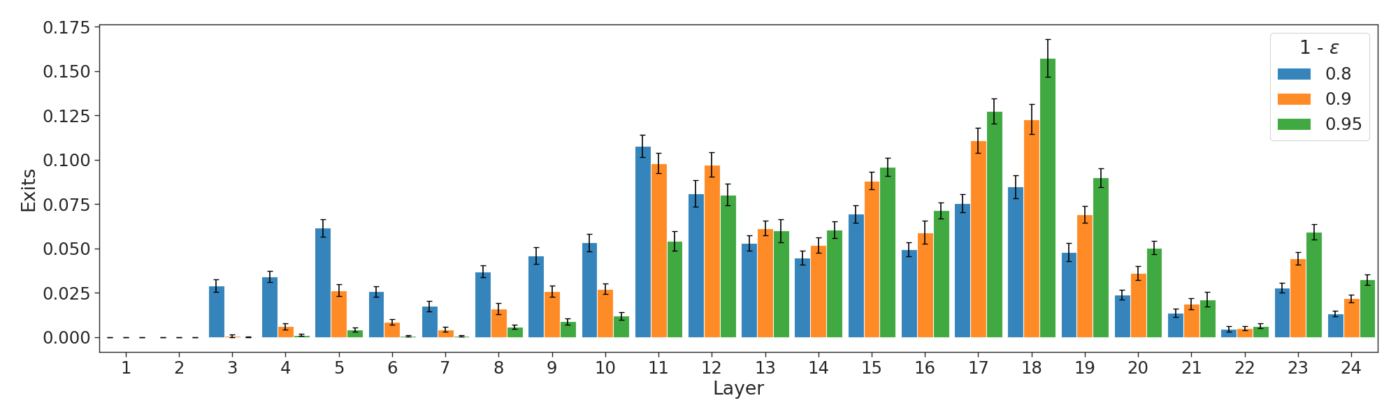
(a) VitaminC

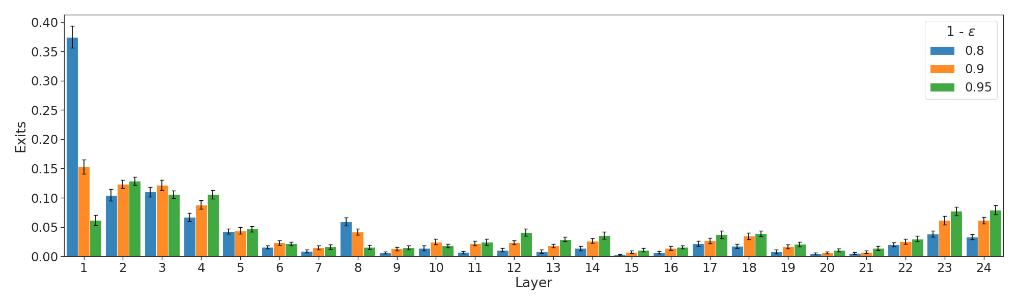
(b) AG News

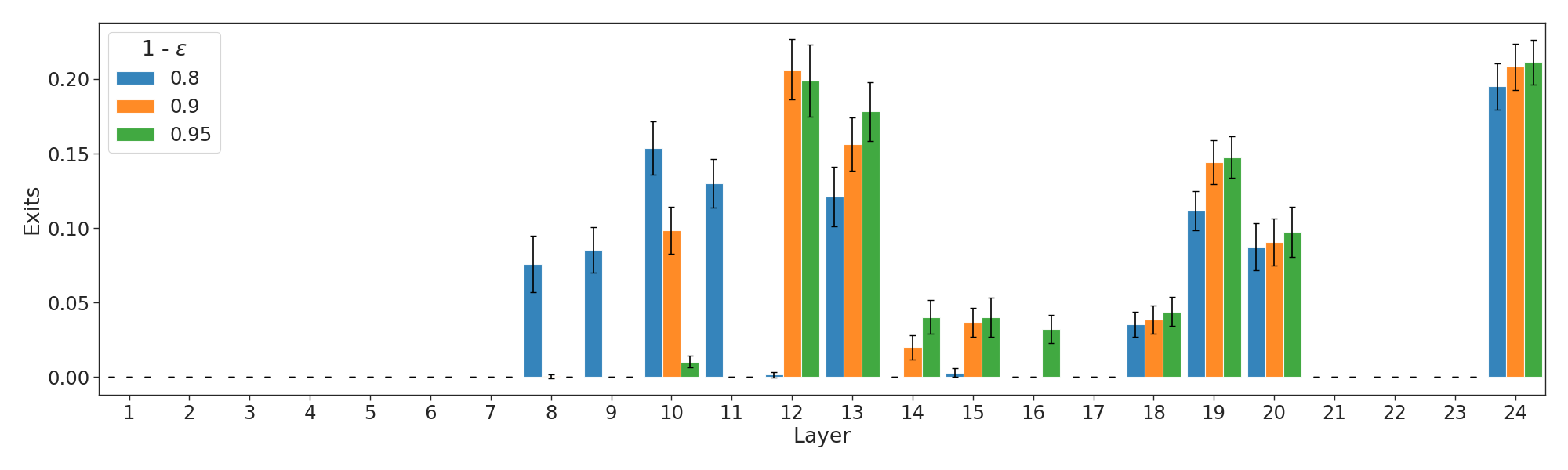
(c) STS-B

Figure C.1: Distribution of exit layers per tolerance level $\epsilon$ (dev sets) with our Shared/ Meta Albert-xlarge model.
See Figure 5 for IMDB.

C.3 Exit layer statistics

Figure C.1 depicts the distribution of exit layers for the different tasks with three reference tolerance levels. Reducing $\epsilon$ requires greater confidence before exiting, resulting in later exits on average. We provide example inputs with their respective exit layer in Appendix D.

Method	Amortized time ($100\cdot T_{\mathcal{G}}/T_{\mathcal{F}}$)				MACs reduction ($|\mathcal{F}|/|\mathcal{G}|$)
	IMDB	VitaminC	AG News	STS-B	IMDB	VitaminC	AG News	STS-B
Thres./ SM	$85.56$	$102.12$	$112.52$	N/A	$1.45$	$1.20$	$1.08$	N/A
Thres./ Meta	$99.85$	$109.93$	$91.95$	$107.44$	$1.35$	$1.22$	$1.48$	$1.25$
Indep./ Meta	$89.25$	$109.57$	$114.66$	$130.36$	$1.53$	$1.22$	$1.17$	$1.02$
Shared/ SM	$67.22$	$\textbf{90}.\textbf{41}$	$69.99$	N/A	$1.90$	$1.37$	$1.81$	N/A
Shared/ Meta	$\textbf{63}.\textbf{99}\ \%$	$94.97\ \%$	$\textbf{60}.\textbf{56}\ \%$	$\textbf{99}.\textbf{38}\ \%$	$\times\textbf{2}.\textbf{22}$	$\times\textbf{1}.\textbf{43}$	$\times\textbf{2}.\textbf{36}$	$\times\textbf{1}.\textbf{36}$

Table C.2: Complementary results for Table 5 with $1-\epsilon=0.95$.

C.4 Albert-base results

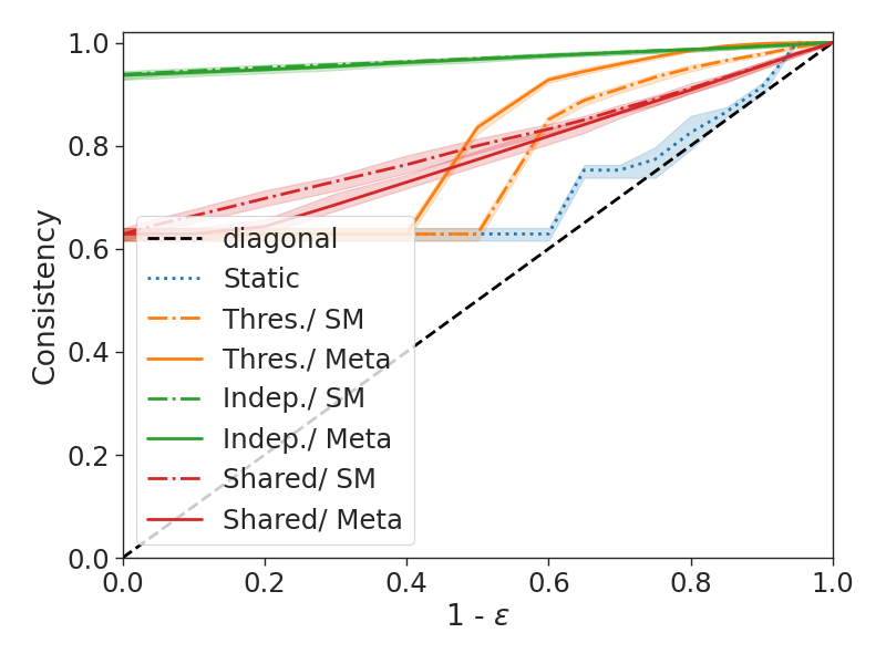
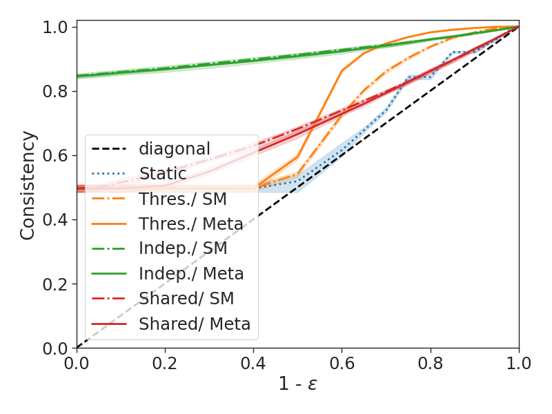
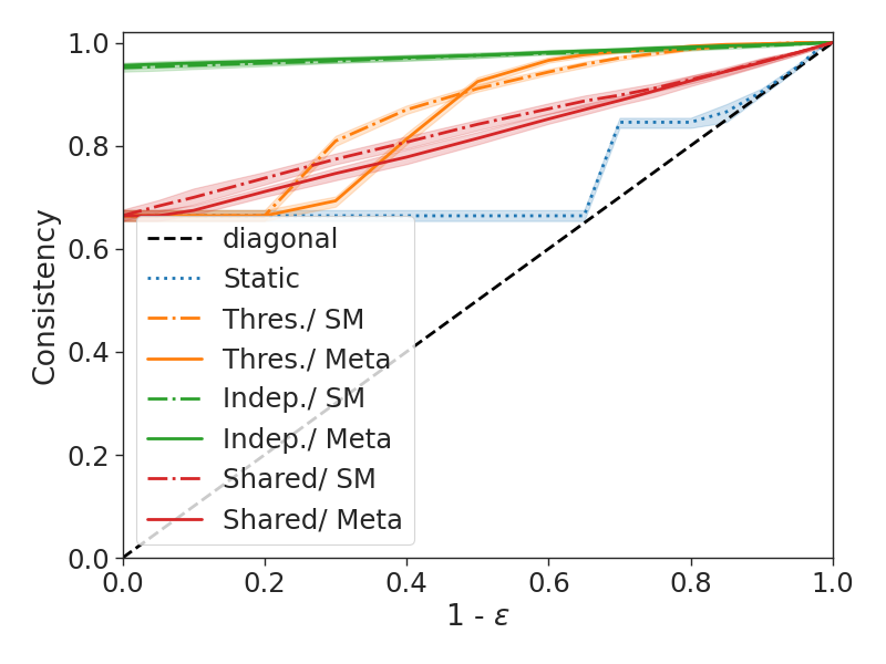
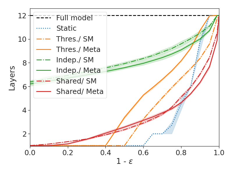
(a) IMDB

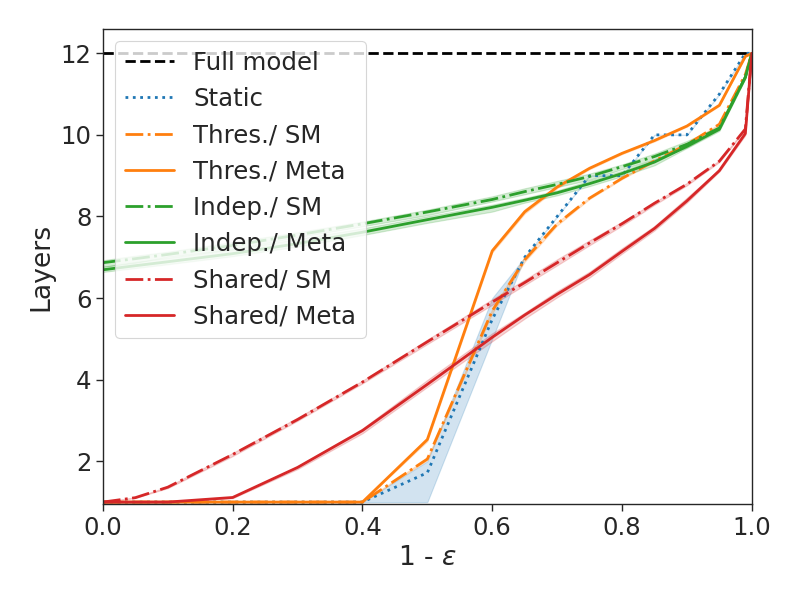
(b) VitaminC

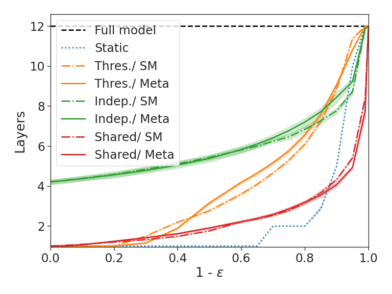
(c) AG News

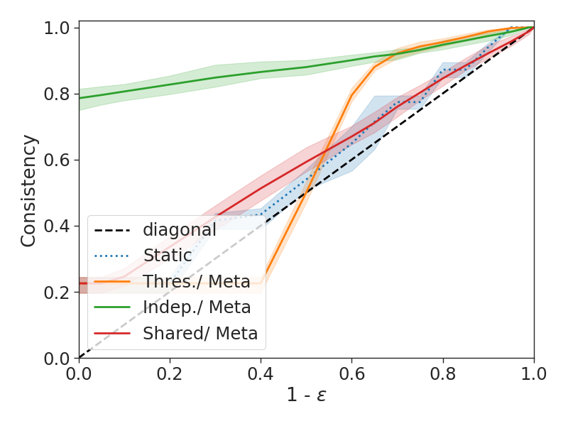
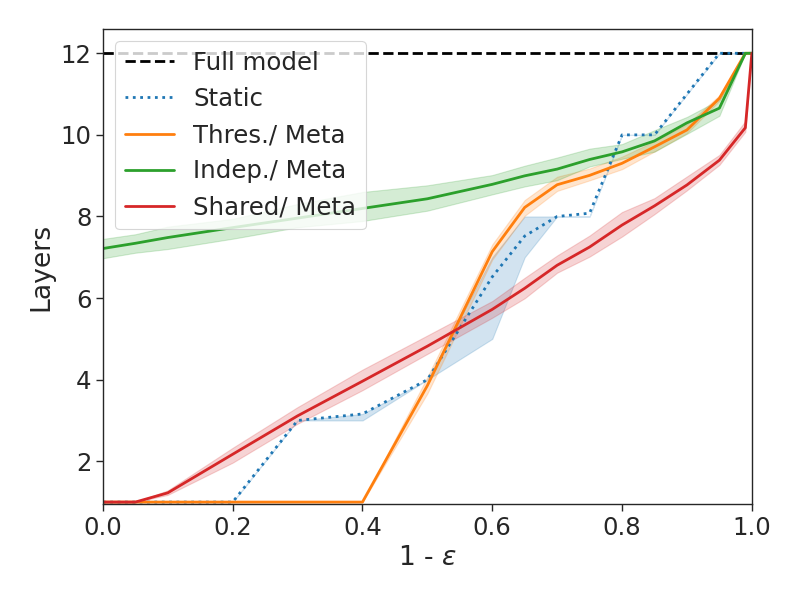
(d) STS-B

Figure C.2: Development set results with an Albert-base 12-layers model as $\mathcal{F}$.

Figure C.2 reports the classification and regression results with an Albert-base 12-layers model. The trends are similar to the larger 24-layers version. Again, we see the efficacy of our Shared conformal calibration and the Meta nonconformity scores. For example, the AG News CAT Shared/ Meta model can preserve 95% consistency while using less than 5 Transformer layers on average.

C.5 RoBERTa-large results

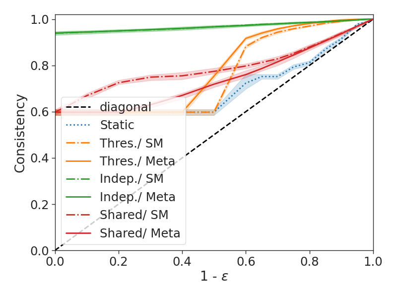
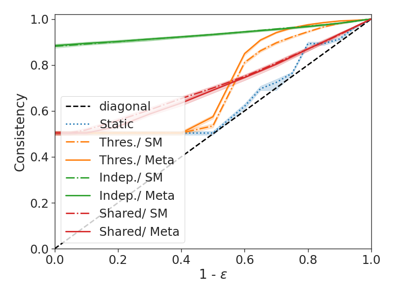
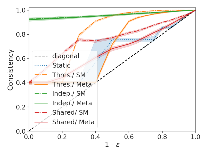
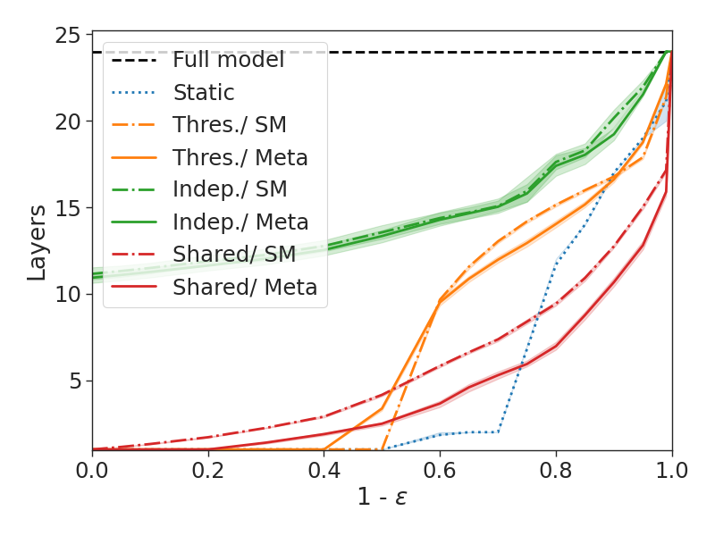
(a) IMDB

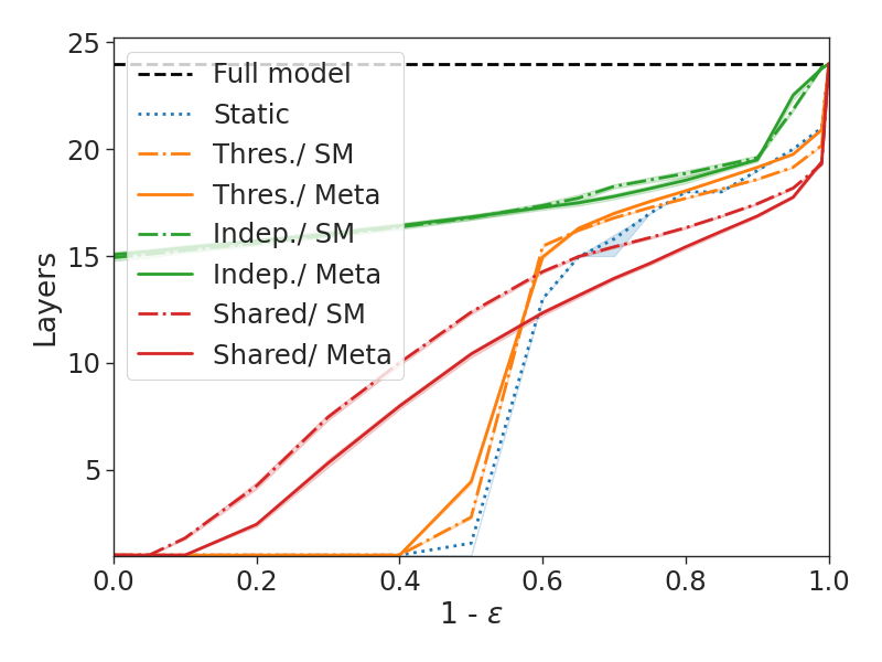
(b) VitaminC

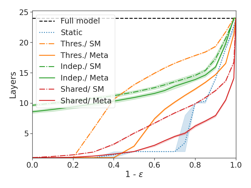
(c) AG News

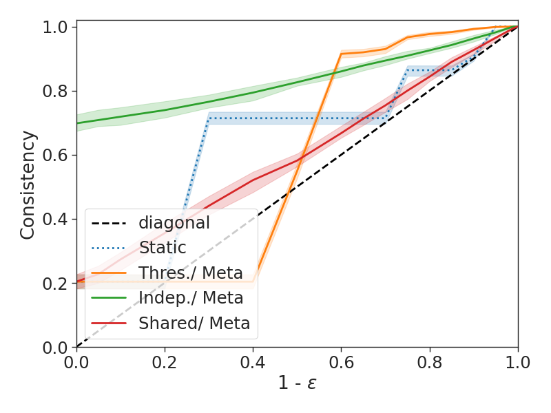
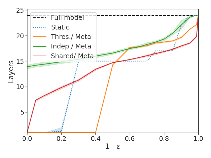
(d) STS-B

Figure C.3: Development set results with an RoBERTa-large 24-layers model as $\mathcal{F}$.

Figure C.3 shows the results of our methods on top of the RoBERTa-large 24-layers Transformer. One main difference between RoBERTa and Albert, is that Albert shares the same parameters across all layers, essentially applying the same function recursively, whereas RoBERTa learns different parameters per layer. Yet, our method is agnostic to such differences and, as observed in the plots, results in similar trends. The value of our Meta classifier compared to the softmax response is even greater with the RoBERTa model.

Appendix D Example Predictions

Table D.1 reports examples of inputs for different tasks and the number of layers that our Albert-xlarge CAT with $\epsilon=0.1$ required. These examples suggest that “easier” inputs (e.g., containing cue phrases or having large overlaps in sentence-pair tasks) might require less layers. In contrast, more complicated inputs (e.g., using less common language or requiring numerical analysis) can lead to additional computational effort until the desired confidence is obtained.

Exit layer	Gold label	Input
	IMDB (Maas et al., 2011)
1	Pos	Without question, film is a powerful medium, more so now than ever before, due to the accessibility of DVD/video, which gives the filmmaker the added assurance that his story or message is going to be seen by possibly millions of people. […]
4	Neg	This movie was obscenely obvious and predictable. The scenes were poorly written and acted even worse.
10	Pos	I think Gerard’s comments on the doc hit the nail on the head. Interesting film, but very long. […]
15	Pos	here in Germany it was only shown on TV one time. today, as everything becomes mainstream, it’s absolute impossible, to watch a film like this again on the screen. maybe it’s the same in USA […]
20	Neg	I tried to be patient and open-minded but found myself in a coma-like state. I wish I would have brought my duck and goose feather pillow… […]
24	Neg	Hypothetical situations abound, one-time director Harry Ralston gives us the ultimate post-apocalyptic glimpse with the world dead, left in the streets, in the stores, and throughout the landscape, sans in the middle of a forgotten desert. […]
	VitaminC (Schuster et al., 2021)
3	Sup	Claim: Another movie titled The SpongeBob Movie: Sponge on the Run is scheduled for release in 2020.
		Evidence: A second film titled The SpongeBob Movie : Sponge Out of Water was released in 2015, and another titled The SpongeBob Movie: Sponge on the Run is scheduled for release in 2020.
5	Sup	Claim: Julie Bishop offered a defence of her nation’s intelligence cooperation with America.
		Evidence: The Australian Foreign Minister Julie Bishop stated that the acts of Edward Snowden were treachery and offered a staunch defence of her nation’s intelligence co-operation with America.
10	NEI	Claim: The character Leslie hurts her head on the window in the film 10 Cloverfield Lane.
		Evidence: Michelle realizes Howard was right and returns his keys.
15	Sup	Claim: Halakha laws are independent of being physically present in the Land of Israel.
		Evidence: The codification efforts that culminated in the Shulchan Aruch divide the law into four sections, including only laws that do not depend on being physically present in the Land of Israel.
20	Sup	Claim: Germany has recorded less than 74,510 cases of coronavirus , including under 830 deaths.
		Evidence: 74,508 cases have been reported with 821 deaths and approximately 16,100 recoveries.
24	NEI	Claim: For the 2015-16 school year , the undergraduate fee at USF is under $43,000.
		Evidence: Undergraduate tuition at USF is $44,040 for the 2016-17 school year.
	AG News (Gulli, 2004; Zhang et al., 2015)
1	Business	Crude Oil Rises on Speculation Cold Weather May Increase Demand Crude oil futures are headed for their biggest weekly gain in 21 months […]
5	Sports	NHL Owner Is Criticized for Talking of Replacement Players The day before the regular season was supposed to open […]
15	World	Scotch Whisky eyes Asian and Eastern European markets (AFP) AFP - A favourite tipple among connoisseurs the world over, whisky is treated with almost religious reverence on the Hebridean […]
20	Business	Arthritis drug withdrawn after trial A prescription painkiller used by more than 250,000 Australians to treat arthritis has been withdrawn from sale after a clinical trial found it doubled the risk […]
24	Sci/Tech	Airbus drops out of Microsoft appeal Aircraft builder withdraws its request to intervene in Microsoft’s antitrust appeal; Boeing also forgoes intervention.
	STS-B (Cer et al., 2017)
10	0.6	Sent. 1: A child wearing blue and white shorts is jumping in the surf.
		Sent. 2: A girl wearing green twists something in her hands.
15	2.8	Sent. 1: Saudi Arabia gets a seat at the UN Security Council
		Sent. 2: Saudi Arabia rejects seat on UN Security Council
20	4.2	Sent. 1: a small bird sitting on a branch in winter.
		Sent. 2: A small bird perched on an icy branch.
24	3.0	Sent. 1: It depends entirely on your company and your contract.
		Sent. 2: It depends on your company.

Table D.1: Number of Transformer layers used for example inputs from the task’s test sets with our Shared/Meta CAT with a tolerance level of $\epsilon=0.1$

References

- Bates et al. (2020) Stephen Bates, Anastasios Nikolas Angelopoulos, Lihua Lei, Jitendra Malik, and Michael I. Jordan. 2020. Distribution free, risk controlling prediction sets. arXiv preprint: arXiv 2101.02703.
- Brown et al. (2020) Tom Brown, Benjamin Mann, Nick Ryder, Melanie Subbiah, Jared D Kaplan, Prafulla Dhariwal, Arvind Neelakantan, Pranav Shyam, Girish Sastry, Amanda Askell, Sandhini Agarwal, Ariel Herbert-Voss, Gretchen Krueger, Tom Henighan, Rewon Child, Aditya Ramesh, Daniel Ziegler, Jeffrey Wu, Clemens Winter, Chris Hesse, Mark Chen, Eric Sigler, Mateusz Litwin, Scott Gray, Benjamin Chess, Jack Clark, Christopher Berner, Sam McCandlish, Alec Radford, Ilya Sutskever, and Dario Amodei. 2020. Language models are few-shot learners. In Advances in Neural Information Processing Systems, volume 33, pages 1877–1901. Curran Associates, Inc.
- Cauchois et al. (2021) Maxime Cauchois, Suyash Gupta, and John C. Duchi. 2021. Knowing what you know: valid and validated confidence sets in multiclass and multilabel prediction. Journal of Machine Learning Research, 22(81):1–42.
- Cer et al. (2017) Daniel Cer, Mona Diab, Eneko Agirre, Iñigo Lopez-Gazpio, and Lucia Specia. 2017. SemEval-2017 task 1: Semantic textual similarity multilingual and crosslingual focused evaluation. In Proceedings of the 11th International Workshop on Semantic Evaluation (SemEval-2017), pages 1–14, Vancouver, Canada. Association for Computational Linguistics.
- Clopper and Pearson (1934) C. J. Clopper and E. S. Pearson. 1934. The use of confidence or fiducial limits illustrated in the case of the binomial. Biometrika, 26(4):404–413.
- Devlin et al. (2019) Jacob Devlin, Ming-Wei Chang, Kenton Lee, and Kristina Toutanova. 2019. BERT: Pre-training of deep bidirectional transformers for language understanding. In Proceedings of the 2019 Conference of the North American Chapter of the Association for Computational Linguistics: Human Language Technologies, Volume 1 (Long and Short Papers), pages 4171–4186, Minneapolis, Minnesota. Association for Computational Linguistics.
- Fan et al. (2020) Angela Fan, Edouard Grave, and Armand Joulin. 2020. Reducing transformer depth on demand with structured dropout. In International Conference on Learning Representations (ICLR).
- Fisch et al. (2021a) Adam Fisch, Tal Schuster, Tommi Jaakkola, and Regina Barzilay. 2021a. Efficient conformal prediction via cascaded inference with expanded admission. In International Conference on Learning Representations (ICLR).
- Fisch et al. (2021b) Adam Fisch, Tal Schuster, Tommi Jaakkola, and Regina Barzilay. 2021b. Few-shot conformal prediction with auxiliary tasks. In International Conference on Machine Learning (ICML).
- Gal and Ghahramani (2016) Yarin Gal and Zoubin Ghahramani. 2016. Dropout as a bayesian approximation: Representing model uncertainty in deep learning. In International Conference on Machine Learning (ICML), volume 48 of Proceedings of Machine Learning Research, pages 1050–1059. PMLR.
- Geifman and El-Yaniv (2017) Yonatan Geifman and Ran El-Yaniv. 2017. Selective classification for deep neural networks. In Advances in Neural Information Processing Systems, volume 30.
- Geng et al. (2021) Shijie Geng, Peng Gao, Zuohui Fu, and Yongfeng Zhang. 2021. Romebert: Robust training of multi-exit bert.
- Graves (2017) Alex Graves. 2017. Adaptive computation time for recurrent neural networks.
- Gulli (2004) Antonio Gulli. 2004. Ag’s corpus of news articles.
- Guo et al. (2017) Chuan Guo, Geoff Pleiss, Yu Sun, and Kilian Q. Weinberger. 2017. On calibration of modern neural networks. In International Conference on Machine Learning (ICML), volume 70, pages 1321–1330, International Convention Centre, Sydney, Australia. PMLR.
- Guo (2017) Hongyu Guo. 2017. A deep network with visual text composition behavior. In Proceedings of the 55th Annual Meeting of the Association for Computational Linguistics (Volume 2: Short Papers), pages 372–377, Vancouver, Canada. Association for Computational Linguistics.
- He et al. (2015) Kaiming He, Xiangyu Zhang, Shaoqing Ren, and Jian Sun. 2015. Deep residual learning for image recognition.
- Huang et al. (2018) Gao Huang, Danlu Chen, Tianhong Li, Felix Wu, Laurens van der Maaten, and Kilian Weinberger. 2018. Multi-scale dense networks for resource efficient image classification. In International Conference on Learning Representations (ICLR).
- Kahneman (2011) Daniel Kahneman. 2011. Thinking, fast and slow. Farrar, Straus and Giroux, New York.
- Kaya et al. (2019) Yigitcan Kaya, Sanghyun Hong, and Tudor Dumitras. 2019. Shallow-deep networks: Understanding and mitigating network overthinking. In International Conference on Machine Learning (ICML), volume 97, pages 3301–3310. PMLR.
- Kingma and Ba (2015) Diederik P. Kingma and Jimmy Ba. 2015. Adam: A method for stochastic optimization. In International Conference on Learning Representations (ICLR).
- Lan et al. (2020) Zhenzhong Lan, Mingda Chen, Sebastian Goodman, Kevin Gimpel, Piyush Sharma, and Radu Soricut. 2020. Albert: A lite bert for self-supervised learning of language representations. In International Conference on Learning Representations (ICLR).
- Langford (2005) John Langford. 2005. Tutorial on practical prediction theory for classification. Journal of Machine Learning Research, 6(10):273–306.
- Lei and Candès (2020) Lihua Lei and Emmanuel Candès. 2020. Conformal inference of counterfactuals and individual treatment effects.
- Liu et al. (2020) Weijie Liu, Peng Zhou, Zhiruo Wang, Zhe Zhao, Haotang Deng, and Qi Ju. 2020. FastBERT: a self-distilling BERT with adaptive inference time. In Proceedings of the 58th Annual Meeting of the Association for Computational Linguistics, pages 6035–6044, Online. Association for Computational Linguistics.
- Liu et al. (2019) Yinhan Liu, Myle Ott, Naman Goyal, Jingfei Du, Mandar Joshi, Danqi Chen, Omer Levy, Mike Lewis, Luke Zettlemoyer, and Veselin Stoyanov. 2019. Roberta: A robustly optimized bert pretraining approach.
- Maas et al. (2011) Andrew L. Maas, Raymond E. Daly, Peter T. Pham, Dan Huang, Andrew Y. Ng, and Christopher Potts. 2011. Learning word vectors for sentiment analysis. In Proceedings of the 49th Annual Meeting of the Association for Computational Linguistics: Human Language Technologies, pages 142–150, Portland, Oregon, USA. Association for Computational Linguistics.
- Niculescu-Mizil and Caruana (2005) Alexandru Niculescu-Mizil and Rich Caruana. 2005. Predicting good probabilities with supervised learning (icml). In International Conference on Machine Learning (ICML).
- Park et al. (2021) Sangdon Park, Shuo Li, Insup Lee, and Osbert Bastani. 2021. PAC confidence predictions for deep neural network classifiers. In International Conference on Learning Representations.
- Paszke et al. (2019) Adam Paszke, Sam Gross, Francisco Massa, Adam Lerer, James Bradbury, Gregory Chanan, Trevor Killeen, Zeming Lin, Natalia Gimelshein, Luca Antiga, Alban Desmaison, Andreas Kopf, Edward Yang, Zachary DeVito, Martin Raison, Alykhan Tejani, Sasank Chilamkurthy, Benoit Steiner, Lu Fang, Junjie Bai, and Soumith Chintala. 2019. Pytorch: An imperative style, high-performance deep learning library. In Advances in Neural Information Processing Systems, volume 32. Curran Associates, Inc.
- Romano et al. (2020) Yaniv Romano, Rina Foygel Barber, Chiara Sabatti, and Emmanuel Candès. 2020. With malice toward none: Assessing uncertainty via equalized coverage. Harvard Data Science Review.
- Sanh et al. (2020) Victor Sanh, Lysandre Debut, Julien Chaumond, and Thomas Wolf. 2020. Distilbert, a distilled version of bert: smaller, faster, cheaper and lighter.
- Schuster et al. (2021) Tal Schuster, Adam Fisch, and Regina Barzilay. 2021. Get your vitamin c! robust fact verification with contrastive evidence. In North American Chapter of the Association for Computational Linguistics: Human Language Technologies (NAACL-HLT).
- Schwartz et al. (2019) Roy Schwartz, Jesse Dodge, Noah A. Smith, and Oren Etzioni. 2019. Green ai.
- Schwartz et al. (2020) Roy Schwartz, Gabriel Stanovsky, Swabha Swayamdipta, Jesse Dodge, and Noah A. Smith. 2020. The right tool for the job: Matching model and instance complexities. In Proceedings of the 58th Annual Meeting of the Association for Computational Linguistics, pages 6640–6651, Online. Association for Computational Linguistics.
- Shafer and Vovk (2008) Glenn Shafer and Vladimir Vovk. 2008. A tutorial on conformal prediction. Journal of Machine Learning Research (JMLR), 9:371–421.
- Sharir et al. (2020) Or Sharir, Barak Peleg, and Yoav Shoham. 2020. The cost of training nlp models: A concise overview. arXiv preprint: arXiv 2006.06138.
- Teerapittayanon et al. (2017) Surat Teerapittayanon, Bradley McDanel, and H. T. Kung. 2017. Branchynet: Fast inference via early exiting from deep neural networks.
- Vaswani et al. (2017) Ashish Vaswani, Noam Shazeer, Niki Parmar, Jakob Uszkoreit, Llion Jones, Aidan N Gomez, Łukasz Kaiser, and Illia Polosukhin. 2017. Attention is all you need. In Advances in Neural Information Processing Systems (NeurIPS).
- Vovk et al. (2005) Vladimir Vovk, Alex Gammerman, and Glenn Shafer. 2005. Algorithmic Learning in a Random World. Springer-Verlag, Berlin, Heidelberg.
- Wang et al. (2018) Xin Wang, Fisher Yu, Zi-Yi Dou, Trevor Darrell, and Joseph E. Gonzalez. 2018. Skipnet: Learning dynamic routing in convolutional networks. In The European Conference on Computer Vision (ECCV).
- Wolf et al. (2020) Thomas Wolf, Lysandre Debut, Victor Sanh, Julien Chaumond, Clement Delangue, Anthony Moi, Pierric Cistac, Tim Rault, Rémi Louf, Morgan Funtowicz, Joe Davison, Sam Shleifer, Patrick von Platen, Clara Ma, Yacine Jernite, Julien Plu, Canwen Xu, Teven Le Scao, Sylvain Gugger, Mariama Drame, Quentin Lhoest, and Alexander M. Rush. 2020. Transformers: State-of-the-art natural language processing. In Proceedings of the 2020 Conference on Empirical Methods in Natural Language Processing: System Demonstrations, pages 38–45, Online. Association for Computational Linguistics.
- Xin et al. (2020a) Ji Xin, Rodrigo Nogueira, Yaoliang Yu, and Jimmy Lin. 2020a. Early exiting BERT for efficient document ranking. In Proceedings of SustaiNLP: Workshop on Simple and Efficient Natural Language Processing, pages 83–88, Online. Association for Computational Linguistics.
- Xin et al. (2020b) Ji Xin, Raphael Tang, Jaejun Lee, Yaoliang Yu, and Jimmy Lin. 2020b. DeeBERT: Dynamic early exiting for accelerating BERT inference. In Proceedings of the 58th Annual Meeting of the Association for Computational Linguistics, pages 2246–2251, Online. Association for Computational Linguistics.
- Xin et al. (2021) Ji Xin, Raphael Tang, Yaoliang Yu, and Jimmy Lin. 2021. BERxiT: Early exiting for BERT with better fine-tuning and extension to regression. In Proceedings of the 16th Conference of the European Chapter of the Association for Computational Linguistics: Main Volume, pages 91–104, Online. Association for Computational Linguistics.
- Zhang et al. (2015) Xiang Zhang, Junbo Zhao, and Yann LeCun. 2015. Character-level convolutional networks for text classification. In Advances in Neural Information Processing Systems, volume 28. Curran Associates, Inc.
- Zhou et al. (2020) Wangchunshu Zhou, Canwen Xu, Tao Ge, Julian McAuley, Ke Xu, and Furu Wei. 2020. Bert loses patience: Fast and robust inference with early exit. In Advances in Neural Information Processing Systems, volume 33, pages 18330–18341. Curran Associates, Inc.