Electro-optical properties of excitons in Cu₂O quantum wells: I discrete states

Abstract

We present theoretical results of the calculations of optical functions for Cu₂O quantum well (QW) with Rydberg excitons in an external homogeneous electric field of an arbitrary field strength. Two configurations of an external electric field perpendicular and parallel to the QW planes are considered in the energetic region for discrete excitonic states. With the help of the real density matrix approach, which enables the derivation of the analytical expressions for the QW electro-optical functions, absorption spectra are calculated for the case of the excitation energy below the gap energy.

I Introduction

Excitons are of great physical interest since they represent the fundamental optical excitation in semiconductors. In particular, excitons in Cu₂O have attracted lots of attention [1] in recent years due to an experiment, in which the hydrogenlike absorption spectrum of these quasiparticles up to a principal quantum number $n=25$ has been observed [2]. Since 2014 astonishing properties of these giant Rydberg excitons (RE) have been studied mostly in bulk systems in context of their spectroscopic chracteristic as well as their linear and nonlinear interparticle interactions and applications in quantum information technology [3]^-[6]. Most studies of RE in an external electric field are concentrated on the excitation energies below the fundamental gap in Cu₂O [7, 8].

The first experiments related to properties of RE focused on natural Cu₂O bulk crystals due to major difficulties in growing high-quality synthetic samples. In the last few years the technological progress enabled the growth of Cu₂O microcrystals with excellent optical material quality and very low point defect levels [9]. This enabled Cu₂O based low-dimensional systems (quantum wells, wires, and dots) to be realized experimentally [10]^-[13].

Cuprous oxide is a semiconductor characterized by large exciton binding energy and with significant technological importance in applications such as photovoltaics and solar water splitting. It is also a superior material system for quantum optics that might enable observation of Rydberg excitons in nano structures. Motivated by technological development and potential applications, investigations of RE in low dimensional systems have started recently [14, 15, 16]. In our previous papers with the help od real density matrix approach (RDMA) we have considered optical properties of RE in quantum dots and quantum wells (QW)[15] and later we have studied Rydberg magnetoexcitons in QW [16]. The applied approach turned out to be useful to describe the fine structure splitting of excitons lines in absorption spectra for any magnetic field strength. The natural step forward at this moment is to study optical response of RE in quantum wells subjected to an interaction with the electric field.for the excitation energy below the gap. In such a situation one can distinguish two cases regarding directions of this external electric field, which can be oriented parallel or perpendicular to the quantum well layer. The first case resembles that known from the bulk in an electric field of the energy below the gap [7]; the degenerations of excitonic levels are lifted, increasing number of peaks corresponding to increasing state number appears, resonances are shifted and anticrossings of lines are observed. For the electric field perpendicular to the quantum well layer the situation is quite distinct from that in bulk semiconductor. The electron and the hole creating the exciton are attracted by their Coulomb attraction and they are confined in a plane of the quantum well and as a consequence large Stark shifts of excitons absorption peaks appear; this phenomenon is called Quantum-Confined Stark Effect; for recent review see [17, 18]. Bellow we will considered these two cases in details.

The paper is organized as follows. In Sec. II we recall the basic equations of the RDMA, adapted for the case of QWs when an external electric field is applied. The Section II is divided into two parts, where different configurations are considered. In Subs. A we consider vthe case of the electric field applied parallel to the z axis (the growth axis), i.e. perpendicular to the QW planes, and in Subs. B the case of the lateral electric field. In both cases we derive analytical expressions for the QW mean effective electro-susceptibility. Those expressions are then used in Sect. III where detailed calculations for the Cu₂O based QWs are presented. The summary and conclusions of our paper are presented in Sec. IV. The Appendices A,B contain the details of the analytical calculations.

II Theory

We consider a Cu₂O quantum well of thickness $L$, located in the $xy$ plane, with QW surfaces located at $z=\pm L/2$. A linearly polarized electromagnetic wave of the frequency $\omega$ is incident normally on the QW. The wave vector has only one component $\bf{k}=k_{z}$ and the electric field vector ${\bf E}=E_{x}$.

We aim to discuss the changes of the QW optical response when a constant external electric field F is applied. The polarization of electrons and holes induced by this field leads to a significant decrease of the exciton binding energy. As it was pointed out there are two opposite directions in which one can applied an electric field to QW: an external field is parallel to the the layers or with the field is directed perpendicular to the layer. In the following subsections both cases will be discussed. As in the previous papers [15, 16], we use the real density matrix approach for calculating the QW optical functions (absorption, reflection, and transmission). In particular, the RDMA turned out to be appropriate for computing the effects of external fields since it includes both the relative motion of the carriers and the center-of-mass motion, where the interaction with the radiation takes place. This approach allows also for including the band mixing effects originate from lifting degenerations of states caused by an external electric field.

II.1 The electric field parallel to the $z$-axis

We use the RDMA approach, as described in ref. [16] to determine the electro-optical properties. The starting point is the constitutive equation

$$(H_{QW}-\hbar\omega-i{\mit\Gamma})Y=\textbf{ME},$$ (1)

with the two-band QW Hamiltonian

$$\phantom{nucl}H_{QW}=E_{g}+\frac{1}{2m_{e}}\left({\bf p}_{e}-e\frac{{\bf r}_{e}\times{\bf B}}{2}\right)^{2}$$

$$+\frac{1}{2m_{h}}\left({\bf p}_{h}+e\frac{{\bf r}_{h}\times{\bf B}}{2}\right)_{z}^{2}$$

$$+\frac{1}{2m_{h}}\biggl{(}{\bf p}_{h}+e\frac{{\bf r}_{h}\times{\bf B}}{2}\biggr{)}_{\parallel}^{2}$$ (2)

$$+e{\bf F}\cdot({\bf r}_{e}-{\bf r}_{h})+V_{\rm conf}({\bf r}_{e},{\bf r}_{h})-\frac{e^{2}}{4\pi\epsilon_{0}\epsilon_{b}|{\bf r}_{e}-{\bf r}_{h}|},$$

B is the magnetic field vector, ${\bf F}$ the electric field vector, $V_{\rm conf}$ are the surface potentials for electrons and holes, $m_{h},m_{e}$ are the hole and the electron effective masses. We separate the exciton center-of-mass and relative motion, and consider the case of ${\bf B}=0$, for $\textbf{F}\parallel z$ and the dipole density ${\bf M}\parallel{\bf E}$. The electron-hole interaction is used in the two-dimensional approximation which enables to obtain the solutions in an analytical form. The calculations of electro-optical properties become much simpler when we consider a quantum well of parabolic confinement potentials in the form of an harmonic oscillator potential $V_{\rm conf}=\frac{1}{2}m_{e}\omega_{ez}^{2}z_{e}^{2}+\frac{1}{2}m_{h}\omega_{hz}^{2}z_{h}^{2}$, where the energies $\hbar\omega_{ez},\hbar\omega_{hz}$ correspond to the electron and hole barriers. For the considered geometry the QW Hamiltonian has the form

$$\phantom{nuc}H_{\rm QW}=E_{g}+H_{m_{e},\omega_{ez}}^{(1D)}(z_{e})+H_{m_{h},\omega_{hz}}^{(1D)}(z_{h})$$

$$+H_{\rm Coul}^{(2D)}(\hbox{\boldmath$\rho$})+eF(z_{e}-z_{h}),$$

and contains the one-dimensional oscillator Hamiltonians

$$H^{(1D)}_{m,\omega}(z)=\frac{p_{z}^{2}}{2m}+\frac{1}{2}m\omega^{2}z^{2},$$ (3)

and the two-dimensional Coulomb Hamiltonian

$$H_{\rm Coul}^{(2D)}(\hbox{\boldmath$\rho$})=\frac{{\bf p}^{2}_{\parallel}}{2\mu_{\parallel}}-\frac{e^{2}}{4\pi\epsilon_{0}\epsilon_{b}\rho}.$$ (4)

Using the substitution

$$\zeta_{e}=z_{e}+z_{0e},\quad z_{0e}=\frac{eF}{m_{e}\omega_{ez}^{2}},$$

$$\zeta_{h}=z_{h}-z_{0h},\quad z_{0h}=\frac{eF}{m_{h}\omega_{hz}^{2}},$$ (5)

we obtain that the QW Hamiltonian (II.1) can be rewritten as

$$\phantom{nuc}H_{\rm QW}=E_{g}+H_{m_{ez},\omega_{ez}}^{(1D)}(\zeta_{e})+H_{m_{h},\omega_{hz}}^{(1D)}(\zeta_{h})$$

$$+H_{\rm Coul}^{(2D)}(\hbox{\boldmath$\rho$})-\frac{(eF)^{2}}{2m_{e}\omega_{ez}^{2}}-\frac{(eF)^{2}}{2m_{h}\omega_{hz}^{2}}.$$ (6)

Using the long wave approximation we seek solutions of Eq.(1) in the form

$$Y(\rho,\zeta_{e},\zeta_{h})=$$ (7)

$$=E(Z)\sum_{jmN_{e}N_{h}}c_{jmN_{e}N_{h}}\psi_{jm}(\hbox{\boldmath$\rho$})\psi^{(1D)}_{\alpha_{e},N_{e}}(\zeta_{e})\psi^{(1D)}_{\alpha_{h},N_{h}}(\zeta_{h}),$$

where $\psi_{jm}$ are the normalized eigenfunctions of the 2-dimensional Coulomb Hamiltonian,

$$\psi_{jm}(\rho,\phi)=R_{jm}(\rho)\frac{e^{im\phi}}{\sqrt{2\pi}},$$

$$R_{jm}=A_{jm}e^{-2\lambda\rho}(4\lambda\rho)^{|m|}L^{|2m|}_{j}(4\lambda\rho),$$ (8)

$$\lambda=\frac{1}{1+2(j+|m|)},$$

$$A_{jm}=\frac{4}{(2j+2|m|+1)^{3/2}}\left[\frac{j!}{(j+2|m|)!}\right]^{1/2},$$

and $L^{\alpha}_{n}(x)$ are the Laguerre polynomials, for which we use the definition

$$L^{\alpha}_{n}(x)={n+\alpha\choose n}M(-n,\alpha+1;x),$$

with the Kummer function $M(a,b,z)$ (the confluent hypergeometric function)[19], $\rho=r/a^{*}$ is the scaled space variable. and $\psi^{(1D)}_{\alpha,N}(z)$ (N=0,1,…) are the quantum oscillator eigenfunctions of the Hamiltonian (3)

$$\psi^{(1D)}_{\alpha,N}(z)=\pi^{-1/4}\sqrt{\frac{\alpha_{z}}{2^{N}N!}}H_{N}(\alpha z)e^{-\frac{\alpha^{2}}{2}z^{2}},$$

$$\alpha=\sqrt{\frac{m\omega_{z}}{\hbar}},$$

with Hermite polynomials $H_{N}(x)$, $(N=0,1,\ldots)$.

Here we use the transition dipole density in the form [16]

$$M(\hbox{\boldmath$\rho$},z_{e},z_{h})=\frac{M_{0}}{2\rho_{0}^{3}}\rho\,e^{-\rho/\rho_{0}}\frac{e^{i\phi}}{\sqrt{2\pi}}\delta(z_{e}-z_{h}).$$ (9)

$M_{0}$ is the integrated strength, the coherence radius is defined $\rho_{0}=r_{0}/a^{*}$, with $r_{0}=\sqrt{\frac{\hbar^{2}}{2\mu E_{g}}}$ and $a^{*}$ is the excitonic Bohr radius. These coefficients are connected through the longitudinal-transversal energy $\Delta_{LT}$

$$(M_{0}\rho_{0})^{2}=\frac{4}{3}\frac{\hbar^{2}}{2\mu}\epsilon_{0}\epsilon_{b}a^{*}\frac{\Delta_{LT}}{R^{*}}\,e^{-4\rho_{0}}.$$ (10)

Assuming that the electromagnetic wave of the component $E(Z)$ is linearly polarized, we substitute $Y$ from Eq. (7) into Eq. (1) to calculate the expansion coefficients $c_{jmN_{e}N_{h}}$

$$\sum_{jmN_{e}N_{h}}c_{jmN_{e}N_{h}}\biggl{[}E_{g}-\hbar\omega-i{\mit\Gamma}$$

$$+\left(N_{e}+\frac{1}{2}\right)\hbar\omega_{ez}+\left(N_{e}+\frac{1}{2}\right)\hbar\omega_{ez}$$ (11)

$$-\frac{(eF)^{2}}{2m_{ez}\omega_{ez}^{2}}-\frac{(eF)^{2}}{2m_{hz}\omega_{hz}^{2}}\biggr{]}\psi_{jm}(\hbox{\boldmath$\rho$})\psi^{(1D)}_{\alpha_{e},N_{e}}(\zeta_{e})\psi^{(1D)}_{\alpha_{h},N_{h}}(\zeta_{h})$$

$$=M(\hbox{\boldmath$\rho$},z_{e},z_{h}),$$

obtaining

$$c_{j1N_{e}N_{h}}=\langle\Psi_{N_{e}N_{h}}\rangle_{\infty}b_{j1}\biggl{[}E_{g}-\hbar\omega-i{\mit\Gamma}+W_{N_{e}}+W_{N_{h}}$$

$$-\frac{(eF)^{2}}{2m_{ez}\omega_{ez}^{2}}-\frac{(eF)^{2}}{2m_{hz}\omega_{hz}^{2}}\biggr{]}^{-1},$$

with the following definitions

$$\langle\Psi_{N_{e}N_{h}}\rangle_{\infty}=\int_{-\infty}^{\infty}\psi^{(1D)}_{\alpha_{e},N_{e}}(\zeta_{e})\psi^{(1D)}_{\alpha_{h},N_{h}}(\zeta_{h})dz$$ (12)

$$=\sqrt{\frac{\alpha_{e}\alpha_{h}}{\pi\,2^{N_{e}+N_{h}}N_{e}!\;N_{h}!}}$$

$$\times\int\limits_{-\infty}^{\infty}dz\biggl{\{}\,H_{N_{e}}[\alpha_{e}(z+z_{0e})]e^{-\frac{\alpha_{e}^{2}(z+z_{0e})^{2}}{2}}$$

$$\times\,H_{N_{h}}[\alpha_{h}(z-z_{0h})]e^{-\frac{\alpha_{h}^{2}(z-z_{0h})^{2}}{2}}\biggr{\}},$$

$$W_{N_{e}}=\left(N_{e}+\frac{1}{2}\right)\hbar\omega_{ez},$$

$$W_{N_{h}}=\left(N_{h}+\frac{1}{2}\right)\hbar\omega_{hz},$$

$$b_{j1}=\frac{2\mu}{\hbar^{2}}\left\{(M_{0}\rho_{0})\frac{6}{\sqrt{2}}\right.$$ (13)

$$\left.\times\sqrt{\frac{(j+1)(j+2)}{(j+3/2)^{5}}}(1+2\rho_{0}\lambda_{j1})^{-4}F\left(-j,4;3;\frac{1}{s}\right)\right\}$$

$$s=\frac{1+2\rho_{0}\lambda_{j1}}{4\rho_{0}\lambda_{j1}},$$

$$\lambda_{j1}=\frac{1}{2j+3},$$

and $F(\alpha,\beta;\gamma;z)$ denotes a hypergeometric series[19] (in Ref.[16] the calculation of $b_{j1}$ is elaborately presented). In the RDMA, the total polarization of the medium is related to the coherent amplitude $Y$ by

$${\bf P}({\bf R})=2\hbox{Re}\int d^{3}{r}\,{\bf M}({\bf r})Y({\bf R},{\bf r})$$ (14)

where R is the center-of-mass coordinate. This, in turn, is used in the Maxwell’s equation

$$c^{2}\nabla^{2}{\bf E(R)}-\epsilon_{b}\ddot{\bf E}=\frac{1}{\epsilon_{0}}{\bf\ddot{P}(R)}.$$ (15)

Using the long wave approximation we obtain the coherent amplitude $Y$ from Eq. (1) as linearly dependent on the electric field E. Then, from Eq. (14), one can determine the susceptibility $\chi(\textbf{R})$[16].

For linearly polarized wave, in the considered configuration for the wave propagating in the $z$-direction, we consider one component $E(Z)$ and one $P(Z)$ of the electric and polarization vectors, obtaining the position-dependent susceptibility $\chi(Z)=\frac{P(Z)}{\epsilon_{0}E(Z)}$.   Below we will use the mean effective QW susceptibility

$$\chi=\frac{1}{L}\int\limits_{-L/2}^{L/2}\frac{P(Z)}{\epsilon_{0}E(Z)}\;dz.$$ (16)

For the considered case of the electric field perpendicular to the QW layer, the polarization determined from Eq. (14), regarding also the form of M, has the form

$$P(Z)=2M_{0}\sum\limits_{N_{e}=0}^{N_{\hbox{\tiny{\emph{e} max}}}}\sum\limits_{N_{h}=0}^{N_{\hbox{\tiny{\emph{h} max}}}}\sum\limits_{j=0}^{J}\biggl{\{}c_{j1N_{e}N_{h}}b_{j1}$$

$$\times\psi^{(1D)}_{\alpha_{e},N_{e}}(Z+z_{e0})\psi^{(1D)}_{\alpha_{h},N_{h}}(Z-z_{h0})\biggr{\}}.$$

Here $J$ denotes the upper limit of $j$, which corresponds to the number of excitonic states taken into account. Using Eq. (16) we arrive at the equation determining the mean effective susceptibility for a QW, when the homogeneous electric field F is applied perpendicular to the QW plane

$$\chi^{(2D)}(\omega)=48\epsilon_{b}\frac{\Delta_{LT}}{R^{*}}\left(\frac{a^{*}}{L}\right)\,\sum\limits_{N_{e}=0}^{N_{\hbox{\tiny{\emph{e} max}}}}\sum\limits_{N_{h}=0}^{N_{\hbox{\tiny{\emph{h} max}}}}\sum\limits_{j=0}^{J}$$ (17)

$$\times\frac{f_{j}^{(2D)}\langle\Psi_{N_{e}N_{h}}\rangle_{\infty}\,\langle\Psi_{N_{e}N_{h}}\rangle_{L}}{L(E_{g}-\hbar\omega+E_{j1}+W_{N_{e}}+W_{N_{h}}+\Delta E-i{\mit\Gamma}_{jN_{e}N_{h}})},$$

where

$$f_{j1}^{(2D)}={48}\frac{(j+1)(j+2)}{\left(j+\frac{3}{2}\right)^{5}}\frac{\left[F\left(-j,4;3;\frac{4\lambda_{j1}\rho_{0}}{1+2\lambda_{j1}\rho_{0}}\right)\right]^{2}}{(1+2\lambda_{j1}\rho_{0})^{8}},$$

$$E_{jm}=-\frac{4}{(2j+2|m|+1)^{2}}R^{*},$$ (18)

$$\langle\Psi_{N_{e}N_{h}}\rangle_{L}=$$

$$=\sqrt{\frac{\alpha_{e}\alpha_{h}}{\pi\,2^{N_{e}}N_{e}!\;2^{N_{h}}N_{h}!}}\int_{-L/2}^{L/2}dz\,\biggl{\{}H_{N_{e}}(z+z_{0e})$$

$$\times e^{-\alpha_{e}^{2}(z+z_{0e})^{2}/2}\,H_{N_{h}}(z-z_{0h})e^{-\alpha_{h}^{2}(z-z_{0h})^{2}/2}\biggr{\}},$$

The Stark shift is given by

$$\Delta E=-\frac{e^{2}F^{2}}{2m_{ez}\omega_{ez}^{2}}-\frac{e^{2}F^{2}}{2m_{hz}\omega_{hz}^{2}}.$$ (19)

For further calculations we have to define the confinement parameters $\alpha_{e,\alpha_{h}}$. We identify the oscillator energies $W_{N_{e}=0},W_{N_{h}=0}$ with those of the lowest energies of the infinite well potentials

$$W_{N_{e}=0}=\frac{\hbar^{2}}{2m_{e}}\frac{\pi^{2}}{L^{2}},\quad W_{N_{h}=0}=\frac{\hbar^{2}}{2m_{h}}\frac{\pi^{2}}{L^{2}},$$ (20)

which gives the coefficients

$$\alpha_{e}=\alpha_{h}=\alpha=\frac{1}{a^{*}}\left(\frac{\pi}{L}\right).$$ (21)

With so chosen confinement parameters the explicit expressions for $\langle\Psi_{N_{e}N_{h}}\rangle_{\infty}$ and $\langle\Psi_{N_{e}N_{h}}\rangle_{L}$ for the lowest combinations of the quantum numbers $N_{e},N_{h}$ are derived in Appendix A. The Stark shift (19) expressed by the confinement parameters depends also on the total excitonic mass and the applied field strength $f=\frac{F}{F_{\rm I}}$ ($F_{I}=\frac{R^{*}}{ea^{*}}$ is the ionization field)

$$\Delta E=-\frac{1}{4\pi^{4}}f^{2}\left(\frac{M_{\rm tot}}{\mu}\right)\left(\frac{L}{a^{*}}\right)^{4}\,R^{*}.$$ (22)

For Cu₂O the ionization field is quite large (due to the smallness of the excitonic Bohr radius), so a feasible cases always correspond to $f<<1$. Such range of the field strength is discussed in our paper. As follows from Eq. (17), the applied electric field in this configuration causes the appearance of confinement states with $N_{e}\neq N_{h}$, which, in the model with equal confinement parameters for electron and hole, are absent in the case without field. As illustration, we present the formula for the mean effective electro-susceptibility, where the lowest confinement states $(N_{e}=N_{h}=0),(N_{e}=1,N_{h}=0),(N_{e}=0,N_{h}=1)$, and $J$ 2D exciton states are accounted for

$$\chi^{(2D)}(\omega)$$

$$=\sum\limits_{j=0}^{J}\frac{\epsilon_{b}\Delta_{LT}a^{*}f_{j}^{(2D)}\langle\Psi_{00}\rangle_{\infty}\,\langle\Psi_{00}\rangle_{L}}{L(E_{g}-\hbar\omega+E_{j1}+W_{N_{e}=0}+W_{N_{h}=0}+\Delta E-i{\mit\Gamma}_{j00})}$$

$$+\sum\limits_{j=0}^{J}\frac{\epsilon_{b}\Delta_{LT}a^{*}f_{j}^{(2D)}\langle\Psi_{10}\rangle_{\infty}\,\langle\Psi_{10}\rangle_{L}}{L(E_{g}-\hbar\omega+E_{j1}+W_{N_{e}=1}+W_{N_{h}=0}+\Delta E-i{\mit\Gamma}_{j10})}$$

$$+\sum\limits_{j=0}^{J}\frac{\epsilon_{b}\Delta_{LT}a^{*}f_{j}^{(2D)}\langle\Psi_{01}\rangle_{\infty}\,\langle\Psi_{01}\rangle_{L}}{L(E_{g}-\hbar\omega+E_{j1}+W_{N_{e}=0}+W_{N_{h}=1}+\Delta E-i{\mit\Gamma}_{j01})},$$

The expressions for the quantities $\langle\Psi_{00}\rangle_{\infty}\,\langle\Psi_{00}\rangle_{L},\,\langle\Psi_{10}\rangle_{\infty}\,\langle\Psi_{10}\rangle_{L}$, and $\langle\Psi_{01}\rangle_{\infty}\,\langle\Psi_{01}\rangle_{L}$ are given in the Appendix A. All relevant parameters are summarized in the Table 1; The dissipation constant $\Gamma$ decreases with $j$ according to experimental data in Ref.[2].

Table 1: Band parameter values for Cu₂O, Rydberg energy and excitonic radius calculated from effective masses; masses in free electron mass $m_{0}$, the ionization field $F_{\rm I}=R^{*}/(ea^{*})$

Parameter	Value	Unit	Reference
$E_{g}$	2172.08	meV	[15]
$R^{*}$	87.78	meV	[15]
$\Delta_{LT}$	$1.25\times 10^{-3}$	meV	[15]
$\mit\Gamma$	$3.88/(j+1)^{3}$	meV	[5]
$m_{e}$	1.0	$m_{0}$	[15]
$m_{h}$	0.7	$m_{0}$	[15]
$M_{\hbox{\tiny tot}}$	1.56	$m_{0}$	[15]
$\mu$	0.363	$m_{0}$	[15]
$a^{*}$	1.1	nm	[15]
$r_{0}$	0.22	nm	[15]
$\epsilon_{b}$	7.5		[15]
$F_{\rm I}$	1.02$\times\,10^{3}$	kV/cm

II.2 The electric field parallel to x axis

In this section we will discuss the case of the electric field F applied parallel to the layer and still we will consider the case of the excitation energy $\hbar\omega$ smaller than the band gap. The electric field can be considered as a perturbation and methods similar to that used in our previous papers for the electric field applied to bulk crystal [7] or for the magnetoexcitons in a QW [16] can be used. Assuming the same shape of the confinement parabolic e-h potential and the two-dimensional Coulomb interaction the QW Hamiltonian consists of the following operators

$$H_{\rm QW}=E_{g}+H_{m_{e},\omega_{ez}}^{(1D)}(z_{e})+H_{m_{h},\omega_{hz}}^{(1D)}(z_{h})$$

$$+H_{\rm Coul}^{(2D)}(\hbox{\boldmath$\rho$})+eF(x_{e}-x_{h}).$$ (23)

Considering the term $eF(x_{e}-x_{h})$ as a perturbation, we seek the solution of the constitutive equation in terms of the eigenfunctions of the unperturbed part of the Hamiltonian

$$Y=$$ (24)

$$=\sum\limits_{jmN_{e}N_{h}}c_{jmN_{e}N_{h}}\psi^{(2D)}_{jm}(\rho,\phi)\psi^{(1D)}_{\alpha_{e},N_{e}}(z_{e})\psi^{(1D)}_{\alpha_{h},N_{h}}(z_{h}).$$

The functions are defined in the previous section. Proceeding in similar way as it was done in Subsection A, i.e. substituting the expansion (24) into the constitutive equation (1) with the Hamiltonian (II.2) and the dipole density (9), we arrive to a set of equations for the expansion coefficients

$$\sum\limits_{j=0}^{J-1}\sum\limits_{N_{e}N_{h}}c_{j1N_{e}N_{h}}\kappa^{2}_{j1N_{e}N_{h}}\delta_{ij}\delta_{N_{e}N_{h}}$$

$$+\sum\limits_{j=0}^{J-1}\sum\limits_{N_{e}N_{h}}c_{j0N_{e}N_{h}}V^{10}_{ij}\delta_{N_{e}N_{h}}$$

$$+\sum\limits_{j=0}^{J-1}\sum\limits_{N_{e}N_{h}}c_{j2N_{e}N_{h}}V^{12}_{ij}\delta_{N_{e}N_{h}}$$

$$=\frac{2\mu}{\hbar^{2}}\frac{1}{a^{*}}\langle R_{i1}|M\rangle\langle\Psi_{N_{e}N_{h}}\rangle_{\infty},$$

$$i=0,1,\ldots,J-1,$$

and

$$\sum\limits_{j=0}^{J-1}\sum\limits_{N_{e}N_{h}}c_{j0N_{e}N_{h}}\kappa^{2}_{j0N_{e}N_{h}}\delta_{ij}\delta_{N_{e}N_{h}}$$

$$+2\sum\limits_{j=0}^{J-1}\sum\limits_{N_{e}N_{h}}\,c_{j1N_{e}N_{h}}\,V^{01}_{ij}\delta_{N_{e}N_{h}}=b_{i};$$

$$i=J,J+1,\ldots$$

$$\sum\limits_{j=0}^{J-1}\sum\limits_{N_{e}N_{h}}c_{j2N_{e}N_{h}}\kappa^{2}_{j2N_{e}N_{h}}\delta_{ij}\delta_{N_{e}N_{h}}$$

$$+2\sum\limits_{j=0}^{J-1}\sum\limits_{N_{e}N_{h}}\,c_{j1N_{e}N_{h}}\,V^{21}_{ij}\delta_{N_{e}N_{h}}=b_{i};$$

$$i=2J,2J+1,\ldots$$

where the following definitions were used

$$\kappa^{2}_{jmN_{e}N_{h}^{2}}=\frac{1}{R^{*}}\left(E_{g}-\hbar\omega+E_{jm}+W_{N_{e}}+W_{N_{h}}-i{\mit\Gamma}\right).$$ (26)

$V$ are the matrix elements

$$V_{\ell s}^{01}=\frac{1}{2}f\int\limits_{0}^{\infty}\rho^{2}\,d\rho\,R_{\ell 0}(\rho)R_{s1}(\rho),$$

$$V_{\ell s}^{10}=\frac{1}{2}f\int\limits_{0}^{\infty}\rho^{2}\,d\rho\,R_{\ell 1}(\rho)R_{s0}(\rho),$$ (27)

$$\ell,s=0,1,\ldots,J-1,$$

$$V_{\ell s}^{12}=\frac{1}{2}f\int\limits_{0}^{\infty}\rho^{2}\,d\rho\,R_{\ell 1}(\rho)R_{s2}(\rho).$$

The equations (II.2) form the set of 3$J$ linear algebraic equations. They can be put into a matrix form

$$\underline{\underline{A}}\textbf{X}=\textbf{b},$$

$$\textbf{X}=(x_{1},x_{2},\cdots x_{3J}),$$ (28)

$$\textbf{b}=(b_{1},b_{2},\cdots b_{3J}),$$

where the matrix elements $\underline{\underline{A}}$ and the components of the vector b are defined in Appendix B. With the solutions X one can obtain the expression for the effective QW electro-susceptibility for $F\parallel x$

$$\chi^{(2D)}(\omega)$$ (29)

$$=48\epsilon_{b}\frac{\Delta_{LT}}{R^{*}}\left(\frac{a^{*}}{L}\right)\hbox{erf}\left(\frac{L\sqrt{p}}{2}\right)\frac{\alpha_{e}\alpha_{h}}{p}\sum\limits_{i=1}^{J}b_{i}\,x_{i}.$$

In order to illustrate such approach and to have an extensive insight into this dependence we take the simplest case, when $J=1.$ Here Eq. (II.2) takes the form

$$\left(\begin{array}[]{ccc}\kappa_{01}^{2}&V^{10}_{00}&V^{12}_{00}\\ 2V_{00}^{01}&\kappa_{00}^{2}&0\\ 2V_{00}^{21}&0&\kappa_{02}^{2}\\ \end{array}\right)\left(\begin{array}[]{c}x_{1}\\ x_{2}\\ x_{3}\end{array}\right)=\left(\begin{array}[]{c}b_{1}\\ 0\\ 0\\ \end{array}\right),$$

where

$$\kappa_{00}^{2}=\frac{1}{R^{*}}\left(E_{g}-\hbar\omega-i{\mit\Gamma}_{0}-4R^{*}+W_{e0}+W_{h0}\right)$$

$$=\frac{1}{R^{*}}\left(E_{T0}-E-i{\mit\Gamma}_{0}\right),$$

$$\kappa_{01}^{2}=\frac{1}{R^{*}}\left(E_{g}-\hbar\omega-i{\mit\Gamma}_{1}-\frac{4}{9}R^{*}+W_{e0}+W_{h0}\right)=$$

$$=\frac{1}{R^{*}}\left(E_{T1}-E-i{\mit\Gamma}_{1}\right),$$

$$\kappa_{02}^{2}=\frac{1}{R^{*}}\left(E_{g}-\hbar\omega-i{\mit\Gamma}_{2}-\frac{4}{25}R^{*}+W_{e0}+W_{h0}\right)=$$

$$=\frac{1}{R^{*}}\left(E_{T2}-E-i{\mit\Gamma}_{2}\right).$$

The relevant root is given by

$$x_{1}=\frac{b_{1}\kappa_{00}^{2}\kappa_{02}^{2}}{\Delta},$$ (31)

where

$$\Delta=-E^{3}+E^{2}(E_{T0}+E_{T1}+E_{T2})-E(E_{T1}E_{T0}$$

$$+E_{T2}E_{T0}+E_{T1}E_{T2})+E_{T0}E_{T1}E_{T2}-af^{2},$$

$$E_{Tm}=\frac{1}{R^{*}}(E_{g}+E_{jm}),$$

$$E_{jm}=-\frac{4R^{*}}{(2j+2|m|+1)^{2}},\qquad j=0,\;m=0,1,2,$$

$$a=2\frac{V^{12}_{00}V_{00}^{21}+V_{00}^{01}V^{10}_{00}}{f^{2}}.$$

Above expressions are used to determine the susceptibility (29), which shows resonant behaviour at the energies resulting from the equation

$$\hbox{Re}\,\Delta=0,$$ (32)

which is a 3-rd degree equation for $E=\hbar\omega/R^{*}$. The constant term contains $f^{2}$, so the solutions will also depend on $f^{2}$. Assuming that $f$ is small we can seek solutions $X_{a},X_{b},X_{c}$ near the unperturbed values $E_{T0},E_{T1},E_{T2}$, $X=X_{a}+\delta$, etc. Solving the equation (32) and retaining terms linear in $\delta$ one obtains

$$\delta_{a}=\frac{af^{2}}{X_{a}(X_{b}+X_{c}-X_{a})-X_{b}X_{c}},$$ (33)

and similarly

$$\delta_{b}=\frac{af^{2}}{X_{b}(X_{a}+X_{c}-X_{b})-X_{a}X_{c}},$$

$$\delta_{c}=\frac{af^{2}}{X_{c}(X_{a}+X_{b}-X_{c})-X_{a}X_{b}}.$$ (34)

The above quantities correspond to $m=0,1,2$, which characterize $s$, $p$ and $d$ excitons. Despite the nontrivial form of Eq. (29) and its dependence on field $f$, some general conclusions can be formulated: the energy shift $\delta_{a,b,c}$ is proportional to $f^{2}$, with quantity $\delta$ varies from state to state, whereas in the configuration $\textbf{F}\parallel z$ the Stark shit has a constant sign and depends only on the QW thickness. By substituting the values for Cu₂O, one obtains $X_{a}\approx 21.28$, $X_{b}\approx 17.72,~{}X_{c}=21.56$ and correspondingly $\delta_{a}\approx 1$, $\delta_{b}\approx-13.67$, $\delta_{c}\approx-1.08$. Therefore, the shifts differ by signs (2 negative and 1 positive) and the most significant occurs for $p$ exciton. The anticrossings may originate from the opposite signs of shifts $\delta_{a,b,c}$; When the field strength $f$ increases, for a certain critical value of $f$ the inversion of places appears: the level $p$ will be (in energetic scale) above the level $d$.

III Results and discussion

III.1 The F field perpendicular to the QW layer ($\textbf{F}||z$)

The behaviour of electro-absorption for electric field perpendicular to quantum well layers is quite distinct from that in bulk semiconductors which is a straightforward consequence of the quantum well gist. Vividly speaking an electric field applied perpendicular to the layer pull the hole and electron (forming the exciton) in opposite directions squashing them against walls of quantum well and both particles are strongly attracted by their Coulomb interaction. Taking into account higher excitonic states one can observe that the exciton absorption peaks are broadened and as a consequence of constrains due to QW there appear large Stark shifts (towards lower energies), which is known as the Quantum-Confined Stark Effect.

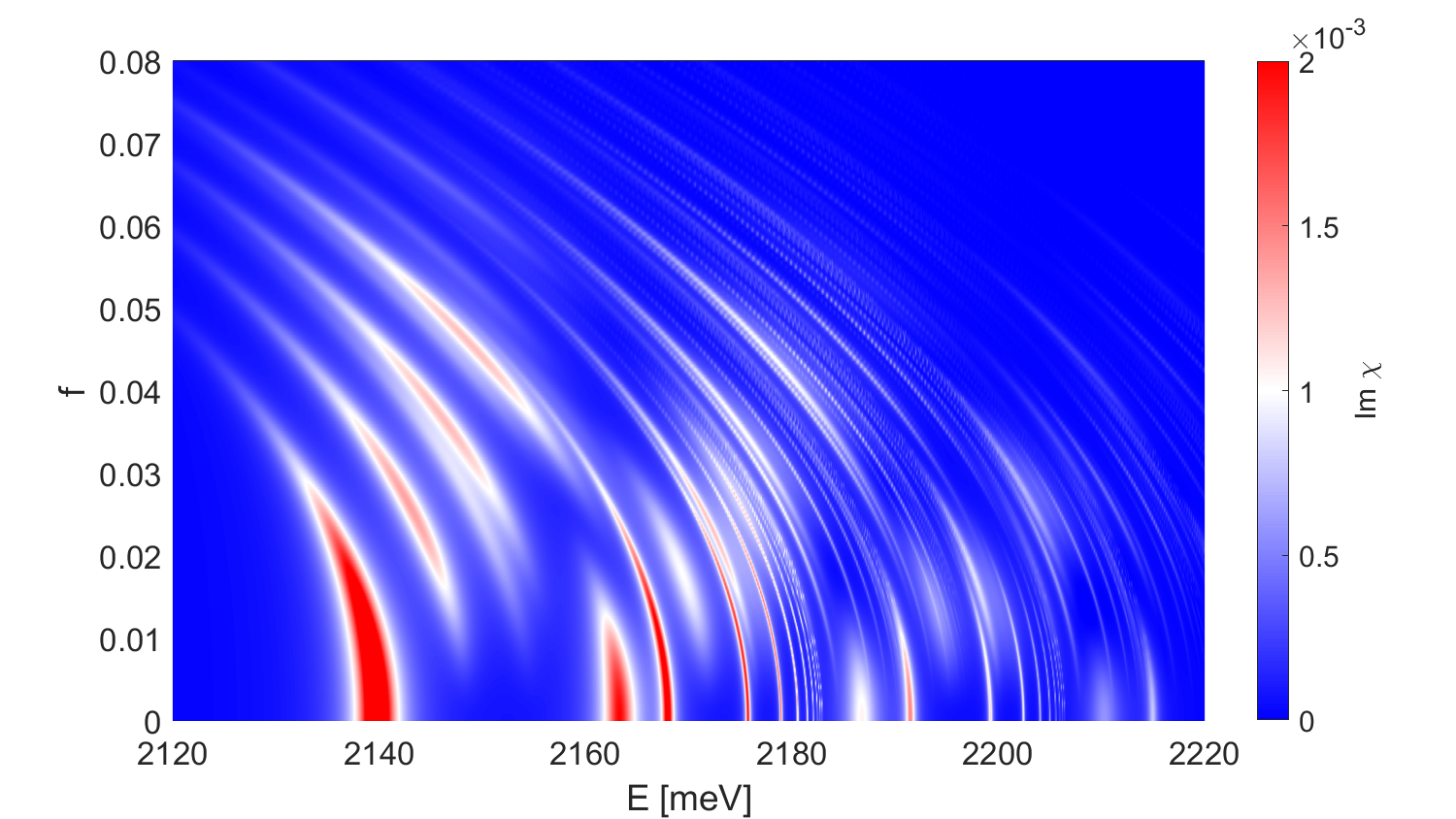
Figure 1: Imaginary part of susceptibility as a function of energy and electric field $f$ for $L$=10 nm.

Fig. 1 shows the imaginary part of susceptibility calculated from Eq. (II.1) for $L=10$ nm and a range of values of electric field. There is a complicated pattern of absorption lines corresponding to various excitonic states $j=0,1,2...$ and confinement states $N_{e}=0,1,2...$ $N_{h}=0,1,2...$. The excitonic number $j$ has the highest impact on linewidth. All resonances experience an energy red-shift proportional to $f^{2}$. One can observe that some states are visible only in some range of values of $f$. In general, lines with higher confinement state numbers are characterized by higher energy and lower amplitude. To identify the particular states, the numbers $[j,N_{e},N_{h}]$ are shown on Fig.2. The identification of states becomes very complicated, due to a large number of overlapping peaks, which is also the case in the bulk crystal [21], but here it turned out to be possible to some extend, i.e., for $j=0,1$ to assign quantum numbers to the resonances. The oscillator strength of the basic excitonic states [0,0,0], [1,0,0] etc. decreases with f. For example, $j=1$ exciton ($\sim 2165$ meV, marked [1,0,0]) and $j=2$ exciton ($\sim 2175$ meV) disappear around $f=0.05$ and $f=0.01$, which corresponds to $51$ kV/cm, and $10$ kV/cm. The latter value can be compared with results presented in [22] and is consistent with them. Overall, the upper limit of considered field values is slightly larger than in available experimental data [8, 21].

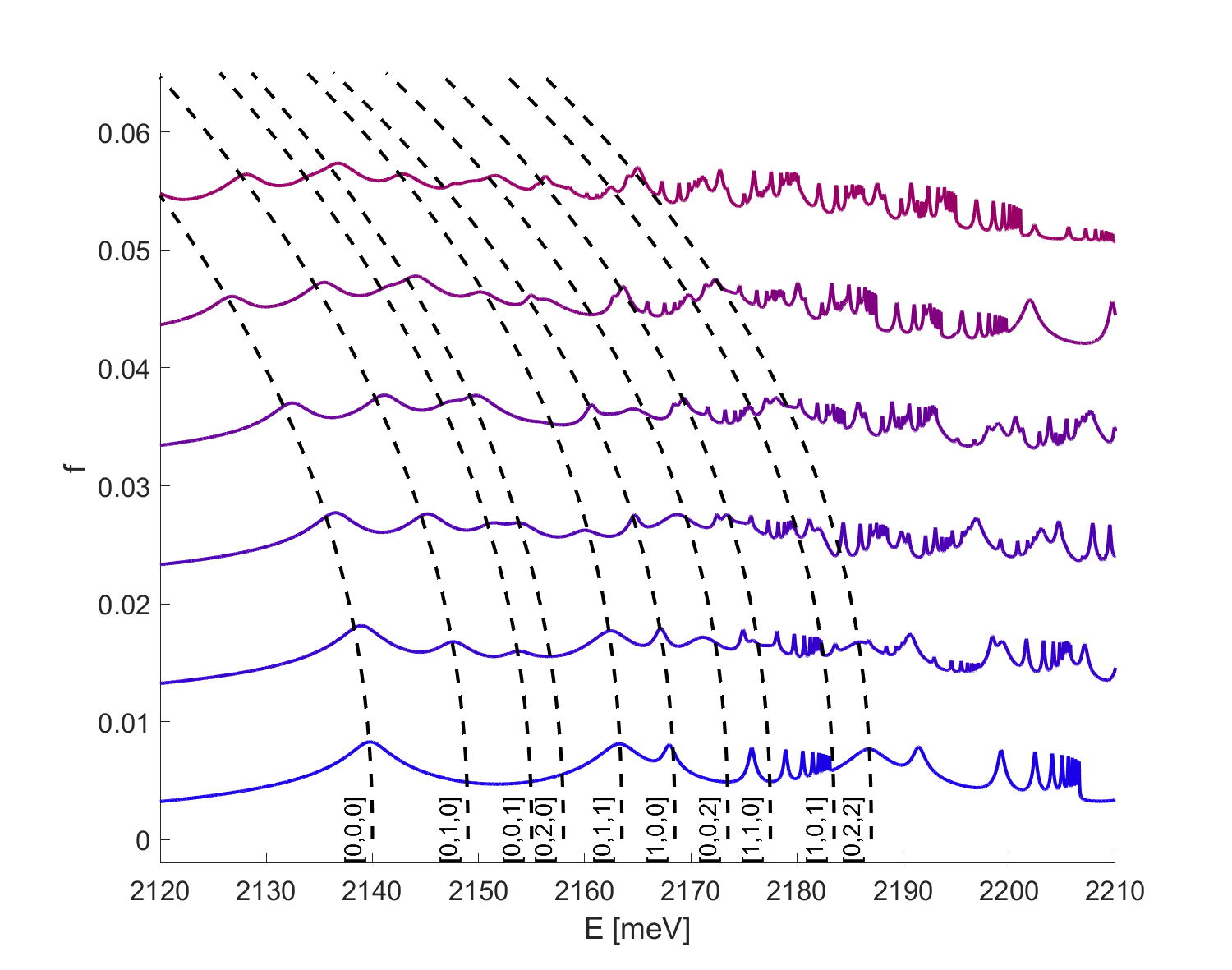
Figure 2: The same as Fig. 1, shown for a few selected values of $f$. Selected lines are marked with dashed lines and identified.

The first line $[0,0,0]$ is a starting point of several series with increasing $j$, $N_{e}$, $N_{h}$. The excitonic states $j$ approach asymptotically a value of $E_{g}^{\prime}\approx 2190$ meV, which is the gap energy with additional shift due to the limited thickness $L=10$ nm. The increase of $N_{e}$ corresponds to the change of energy $\Delta E\sim 8.5$ meV (for example, distance between [0,0,0] and [0,1,0]); the gap between consecutive $N_{h}$ lines ([0,0,0] and [0,0,1]) is roughly $\Delta E\approx 15$ meV. Again, one can see that some lines are visible only in some range of $f$; for example, [0,1,1] disappears around $f\approx 0.035$. The lines corresponding to high values of $j$, $N_{e}$, $N_{h}$ extend beyond the bandgap, creating a very complicated pattern in this region, especially for large values of $f$.

To further explore the impact of confinement quantum numbers on the state energy, the susceptibility has been calculated taking into account only $j=0$ excitonic state. The results are shown on the Fig. 3.

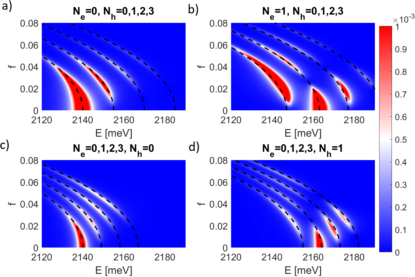
Figure 3: Imaginary part of susceptibility calculated for $L=10$ nm, $j=0$ and a) $N_{e}=0$, b) $N_{e}=1$, c) $N_{h}=0$, d) $N_{h}=1$.

Four different cases are presented where either $N_{e}$ or $N_{h}$ is set to 0 or 1. Fig. 3 a) shows the spectrum for $N_{e}=0$. One can see that the lines corresponding to $N_{h}=1,2,3,4$ are equally spaced and exhibit the same energy shift with $f$. Higher values of $N_{h}$ correspond to weaker lines with higher minimal value of $f$ above which the line becomes visible. The only line present at $f=0$ is $N_{e}=N_{h}=0$. The spectrum becomes slightly more complex when $N_{e}=1$, as shown on Fig. 3 b); with the exception of $N_{h}=0$, the lines split into two ranges of $f$ where they have nonzero amplitude. Again, the amplitude decreases with $N_{h}$ while the energy increases with $N_{h}$ in a linear manner. Fig. 3 c) is very similar to Fig. 3 a), with main difference being smaller energy spacing between $N_{e}=1,2,3,4$ lines. In the same manner, Fig. 3 d) has the same structure as Fig. 3 b). One can see that only $N_{e}=N_{h}$ states are visible for $f=0$. This is also visible on Fig. 2.

The above discussed line series are repeated for every value of excitonic state number $j$. Fig. 4 a) shows the spectrum calculated for $j=0..9$ and $N_{e}=N_{h}=0$. One can see a typical excitonic line series with energy asymptotically approaching some constant value. With increase of either $N_{e}$ (Fig. 4 b)) or $N_{h}$ (Fig. 4 c)), the whole spectrum is shifted in energy and the range of values of $f$ where the lines are visible moves up. Finally, Fig. 4 d) shows the case of various values of $N_{e}=N_{h}=1,2,3,4$; one can observe that every consecutive line splits into more separate parts. By observing higher confinement states, we can conclude that for any combination of $N_{e}$, $N_{h}$, the line splits into $min(N_{e},N_{h})+1$ areas where its amplitude is nonzero.

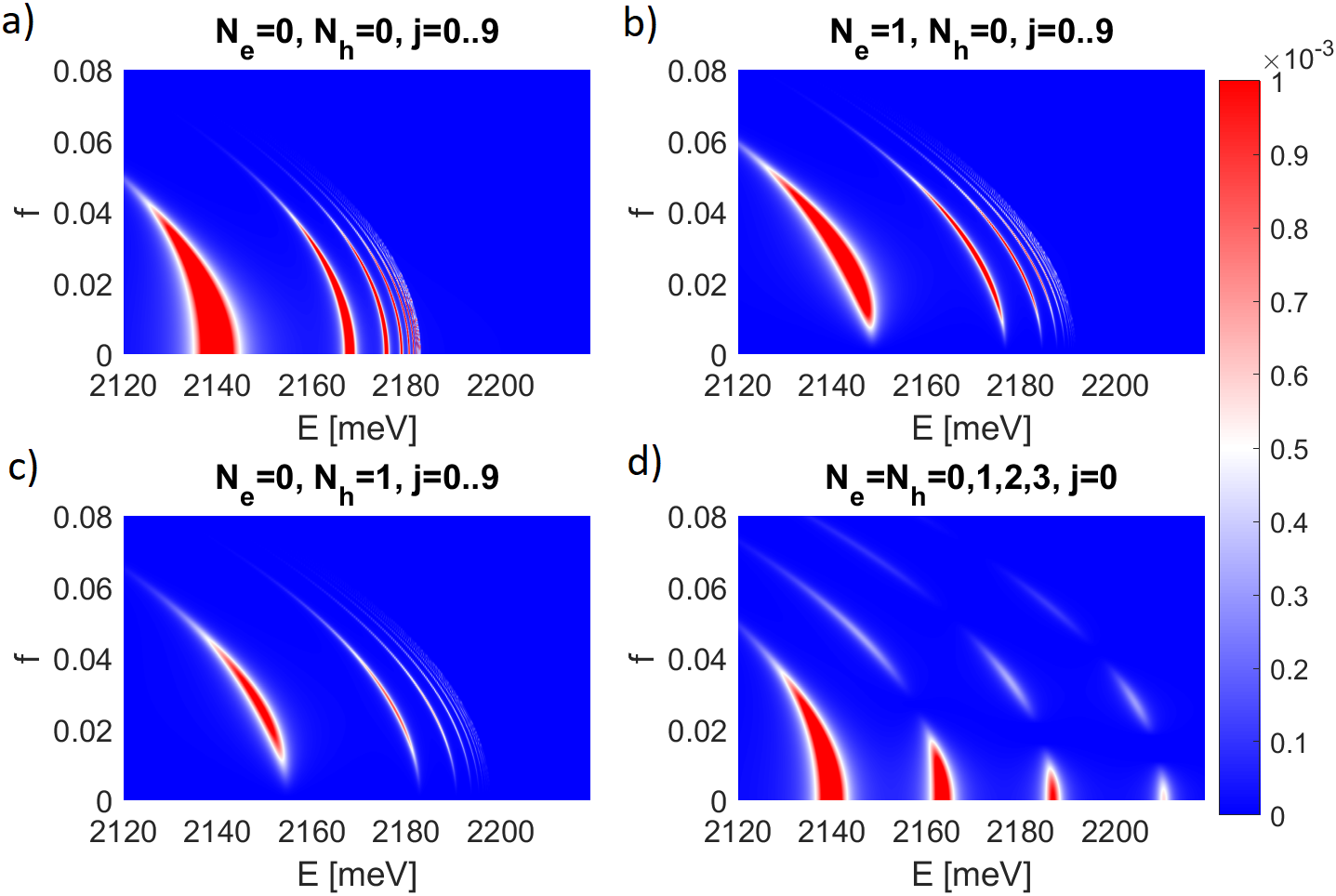
Figure 4: Imaginary part of susceptibility calculated for $L=10$ nm, $j=0..9$ and a) $N_{e}=N_{h}=0$, b) $N_{e}=1$, c) $N_{h}=1$, d) $j=0$,$N_{e}=N_{h}=1,2,3,4$.

Fig. 5 shows the dependence on $L$ for the same confinement state combinations as in Fig. 3. One can see that in all cases, the energy diverges as $L\rightarrow 0$; however, in contrast to the electric field dependence, the speed of divergence and the exact location of asymptote is different for various values of $N_{e}$, $N_{h}$. For example, on Fig. 5 a) the line $N_{h}=0$ approaches infinity as $L\rightarrow 2$ nm, while $N_{h}=3$ diverges at $L\rightarrow 6$ nm. One can also see that the lines corresponding to higher $N_{h}$ are present in a narrower range of values of $L$. The spectrum for $N_{e}=1$ (Fig. 5 b)) exhibits the same split into two ranges of $L$ as in the case of electric field dependence. The minimum thickness where those lines appear is slightly higher than for $N_{e}=0$. Again, Figs. 5 c) and 5 d) are analogous to Figs. 5 a) and 5 b), but with smaller energy spacing between lines.

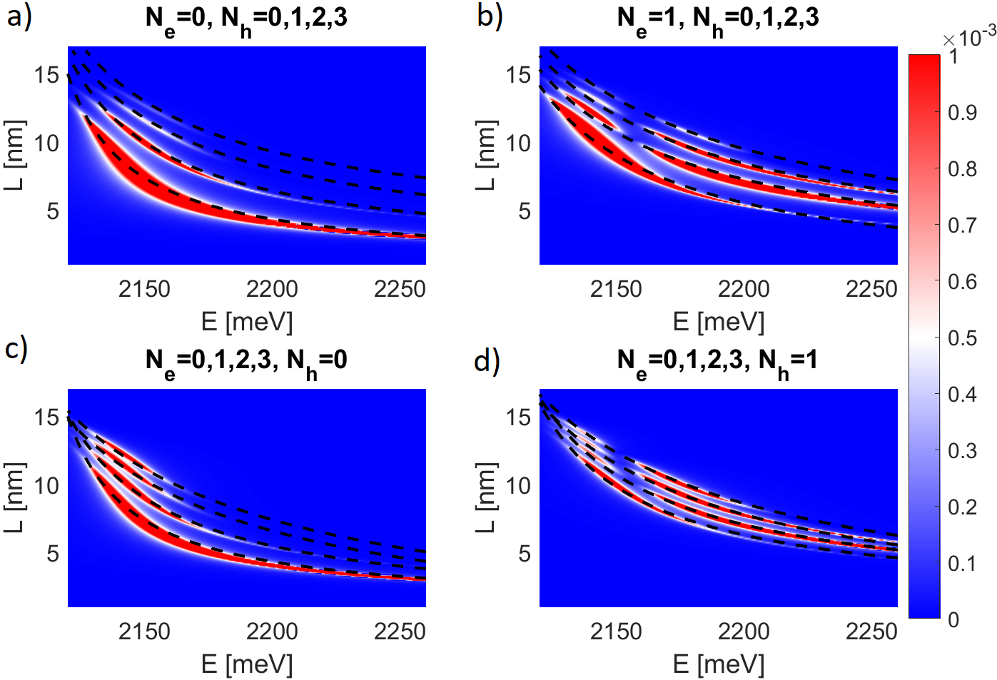
Figure 5: Imaginary part of susceptibility calculated for $L=10$ nm, $j=0$ and a) $N_{e}=0$, b) $N_{e}=1$, c) $N_{h}=0$, d) $N_{h}=1$.

III.2 The F field parallel to the QW layer ($\textbf{F}||x$)

For the case of electric field parallel to the layer we deal with the effects that are qualitatively similar to those seen in the bulk semiconductor. The main observations are lifting degeneracy of excitonic spectrum due to the external field and appearance of avoided crossings.

Fig. 6 presents the absorption spectrum calculated from Eq. (29) for selected values of electric field $f$ and thickness $L$=20 nm.

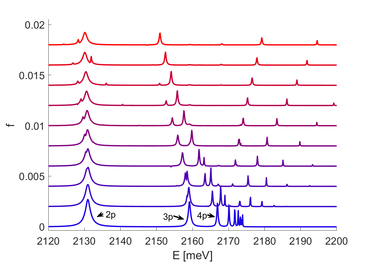
Figure 6: Imaginary part of susceptibility as a function of energy and electric field $f$.

At $f=0$, a standard series of p-exciton lines is visible. One can that the exciton energies approach $E\approx 2175$ meV, which is larger than $E_{g}$ due to the $L$-dependent energy shift. The state $2p$ exhibits very little shift with electric field, but the effect is much stronger for higher states $3p$, $4p$ etc. Due to the fact that the state energy decreases with $f$ and the reduction is faster for upper states, there is a lot of lines overlaps and anticrossing is observed. In the high energy region, multiple small peaks are visible; these maxima correspond to the $d$ excitons, starting from $3d$ levels. Finally, one can observe that the absorption amplitude decreases slowly with electric field. To better understand the structure of the spectrum, a continuous range of values of $f$ is investigated on Fig. 7.

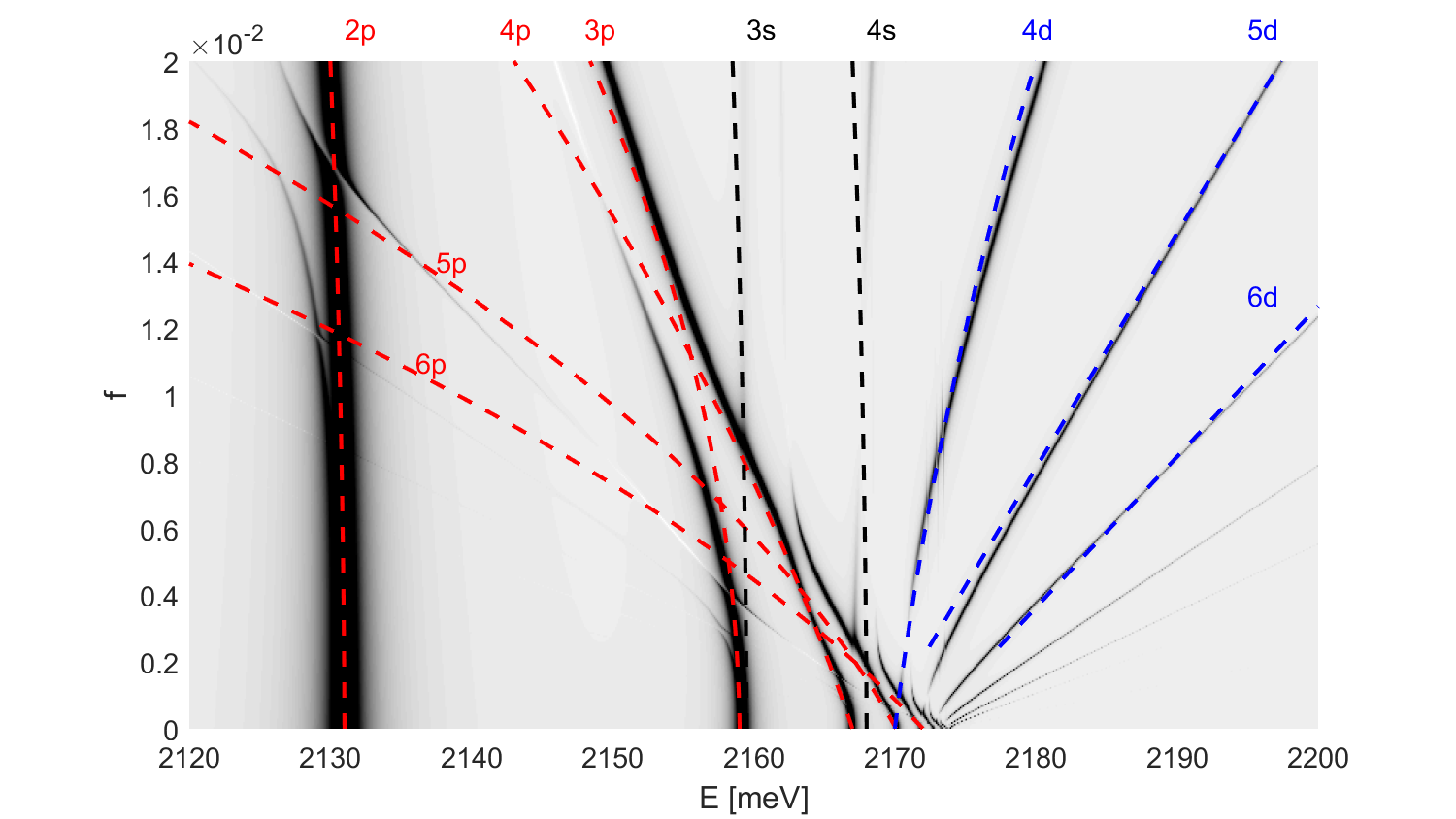
Figure 7: Imaginary part of susceptibility (brightness, in log scale) as a function of energy and electric field $f$.

The $s$, $p$ and $d$ excitons are marked by black, red and blue lines, accordingly. The $p$ excitons exhibit an approximately quadratic energy shift with $f$; due to the line overlap, only $2p$ and $3p$ excitonic lines are clearly visible in the full range of $f$. One can observe a significant anticrossing of $3p$ and $4p$ lines originating from nondiagonal matrix elements in Eq. (II.2). Interestingly, while the $s$ exciton lines are not highly visible, they also cause anticrossings (for example, intersection of $4s$ and $5p$ lines at $f=4\cdot 10^{-3}$). The $d$ exciton lines appear at some minimal value of $f\sim 2\cdot 10^{-3}$ and are linearly upshifted with $f$.

A more detailed analysis of single excitonic state $j=2$ is shown on Fig. 8. The overall spectrum structure follows the one presented in [20]; the strongest $3p$ line (red) starts from $E\approx 2157$ meV and exhibits quadratic energy shift. There is a pair of $3d$ lines which originate from a point $E\approx 2165$ meV and split in a linear manner with f. These lines become visible at $f\sim 2\cdot 10^{-}3$; in a high field regime, their amplitude becomes comparable to the $p$ state. Another feature of the spectrum is a $d$ exciton triplet. Those lines are visible mostly in the region of their anticrossing with $p$ and $s$ state. The $3s$ state is also visible for sufficiently strong field; its energy is almost independent of $f$. Note that while for $f=0$ the $s$-exciton has lower energy than $p$ exciton, the situation reverses for high field due to the fact that the $s$ state very weakly affected by the external field in contrast to the $p$ and $d$ states. Such a phenomenon was observed experimentally in [20].

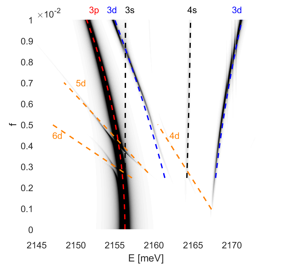
Figure 8: Imaginary part of susceptibility (brightness, in log scale) of the n=3 state as a function of energy and electric field $f$.

Even more complicated spectrum is obtained for $n=5$ state (Fig. 9). In addition to single $p$, single $s$ and two $d$ states, there are multiple apparent lines that can be attributed to anticrossings with $4d$ and $6d$ excitons. For any given $n$, the states form a structure close to the standard Stark fan [8] and its width is comparable with experimental results in [8] for the same electric field value. Again, due to the field-induced downshift, the $5p$ state crosses the lines of $3s$, $4s$ and $5s$ excitons; due to the lower linewidth of $5p$ level, these anticrossings are more apparent.

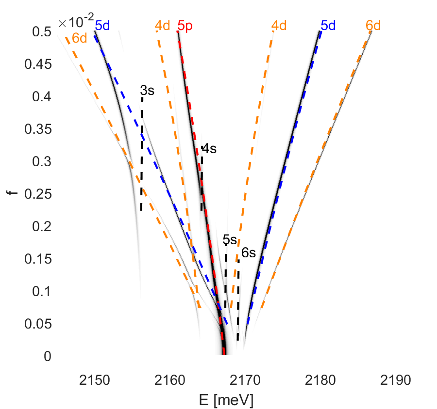
Figure 9: Imaginary part of susceptibility (brightness, in log scale) of the n=5 state as a function of energy and electric field $f$.

Finally, Fig. 10 shows the dependence of exciton energy on the QW thickness $L$, calculated for electric field $f=0.01$. The shift dependence of the lower states is more pronounced for wider quantum wells. Moreover, one can see two series of states: the $p$ excitons and the high-energy $d$ excitons. Both types of states exhibit a strong upshift with reduction of L, approaching $E\rightarrow\infty$ as $L\rightarrow 3$ nm.

Figure 10: Imaginary part of permittivity (color) as a function of energy and well thickness $L$.

IV Conclusions

In this paper we have studied the electro-optical properties of Cu₂O QWs with Rydberg excitons in two different orientations of the applied external electric field, for excitation energies below the fundamental gap. For the electric field applied in the z-direction, and in the considered field strengths range, the quadratic Stark red shift of resonance energies prevails, depending on the QW thickness and the total exciton mass. New resonances appear, which are not allowed, for symmetry reasons, when the electric field is absent. We observe even more complicated dependences in the case of the lateral applied field. The resonances can be both red- and blue shifted. We observe a considerable interlevel mixing and splitting caused by differences in energy shifts and various excitonic states due to the interplay between the confinement influence and the electric field. We believe that tunability of optical properties of QW with RE which is enabled in both electric field configurations makes them suitable for applications as flexible devices in nanotechnology.

Appendix A Quantities $\langle\Psi_{N_{e}N_{h}}\rangle_{\infty},\langle\Psi_{N_{e}N_{h}}\rangle_{L}$

We use the definitions (II.1), (12), and (II.1), to calculate the quantities $\langle\Psi_{NeN_{h}}\rangle_{\infty}$, and $\langle\Psi_{NeN_{h}}\rangle_{L}$. We take three combinations: $N_{e}=0,N_{h}=0$, $N_{e}=1,N_{h}=0$, and $N_{e}=0,N_{h}=1$. Inserting the definitions of the Hermite polynomials $H_{0},H_{1}$, and performing the respective integrations, one obtains

$$\langle\Psi_{00}\rangle_{\infty}=\sqrt{\frac{\alpha_{e}\alpha_{h}}{p}}\exp\left[-\frac{\alpha_{e}^{2}\alpha_{h}^{2}(z_{0e}+z_{0h})^{2}}{2(\alpha_{e}^{2}+\alpha_{h}^{2})}\right],$$ (35)

$$\langle\Psi_{00}\rangle_{L}=\sqrt{\frac{\alpha_{e}\alpha_{h}}{p}}\exp\left[-\frac{\alpha_{e}^{2}\alpha_{h}^{2}(z_{0e}+z_{0h})^{2}}{2(\alpha_{e}^{2}+\alpha_{h}^{2})}\right]$$ (36)

$$\times\frac{1}{2}\biggl{[}\hbox{erf}\left(\frac{L\sqrt{p}}{2}+\frac{q}{\sqrt{p}}\right)+\hbox{erf}\left(\frac{L\sqrt{p}}{2}-\frac{q}{\sqrt{p}}\right)\biggr{]},$$

$$\langle\Psi_{10}\rangle_{\infty}=\frac{\alpha_{e}}{p}\left(\frac{q}{\sqrt{p}}+z_{0e}\sqrt{p}\right)\sqrt{\frac{\alpha_{e}\alpha_{h}}{2}}$$ (37)

$$\times\exp\left[-\frac{\alpha_{e}^{2}\alpha_{h}^{2}(z_{0e}+z_{0h})^{2}}{2(\alpha_{e}^{2}+\alpha_{h}^{2})}\right],$$

$$\langle\Psi_{01}\rangle_{\infty}=\frac{\alpha_{h}}{p}\left(\frac{q}{\sqrt{p}}-z_{0h}\sqrt{p}\right)\sqrt{\frac{\alpha_{e}\alpha_{h}}{2}}$$ (38)

$$\times\exp\left[-\frac{\alpha_{e}^{2}\alpha_{h}^{2}(z_{0e}+z_{0h})^{2}}{2(\alpha_{e}^{2}+\alpha_{h}^{2})}\right],$$

$$\langle\Psi_{10}\rangle_{L}=$$

$$=\frac{\alpha_{e}}{\sqrt{\pi}}\sqrt{\frac{\alpha_{e}\alpha_{h}}{2}}\exp\left[-\frac{\alpha_{e}^{2}\alpha_{h}^{2}(z_{0e}+z_{0h})^{2}}{2(\alpha_{e}^{2}+\alpha_{h}^{2})}\right]$$ (39)

$$\times\frac{1}{2p}\biggl{\{}\exp\left[-\left(\frac{L\sqrt{p}}{2}+\frac{q}{\sqrt{p}}\right)^{2}\right]-\exp\left[\left(\frac{L\sqrt{p}}{2}-\frac{q}{\sqrt{p}}\right)^{2}\right]$$

$$+\left(\frac{q}{\sqrt{p}}+z_{0e}\sqrt{p}\right)\sqrt{\pi}\biggl{[}\hbox{erf}\biggl{(}\frac{L\sqrt{p}}{2}+\frac{q}{\sqrt{p}}\biggr{)}$$

$$+\hbox{erf}\left(\frac{L\sqrt{p}}{2}-\frac{q}{\sqrt{p}}\right)\biggr{]}\biggr{\}}.$$

and

$$\langle\Psi_{01}\rangle_{L}=\langle e0|h1\rangle$$

$$=\frac{\alpha_{h}}{\sqrt{\pi}}\sqrt{\frac{\alpha_{e}\alpha_{h}}{2}}\exp\left[-\frac{\alpha_{e}^{2}\alpha_{h}^{2}(z_{0e}+z_{0h})^{2}}{2(\alpha_{e}^{2}+\alpha_{h}^{2})}\right]$$ (40)

$$\times\frac{1}{2p}\biggl{\{}\exp\left[-\left(\frac{L\sqrt{p}}{2}+\frac{q}{\sqrt{p}}\right)^{2}\right]-\exp\left[\left(\frac{L\sqrt{p}}{2}-\frac{q}{\sqrt{p}}\right)^{2}\right]$$

$$+\left(\frac{q}{\sqrt{p}}-z_{0h}\sqrt{p}\right)\sqrt{\pi}$$

$$\times\left[\hbox{erf}\left(\frac{L\sqrt{p}}{2}+\frac{q}{\sqrt{p}}\right)+\hbox{erf}\left(\frac{L\sqrt{p}}{2}-\frac{q}{\sqrt{p}}\right)\right]\biggr{\}},$$

where erf() is the error function [19]. The quantities $p$ and $q$ are defined as

$$p=\frac{1}{2}\left(\alpha_{e}^{2}+\alpha_{h}^{2}\right),$$

$$q=\frac{1}{2}\left(\alpha_{h}^{2}z_{0h}-\alpha_{e}^{2}z_{0e}\right).$$ (41)

In all the above expressions, due to Eq. (21), one has to put $\alpha_{e}=\alpha_{h}$.

Appendix B Matrix elements for the lateral field

For the sake of simplicity we consider only the lowest confinement state, $N_{e}=N_{h}=0$. Using the notation

$$c_{01}=x_{1},\;c_{11}=x_{2},..,\;c_{J-1,1}=x_{J},\;c_{r-1,1}=x_{r},\;r=1,..,J$$

$$c_{00}=x_{J+1},\;c_{10}=x_{J+2},..,\;c_{r-1,0}=x_{r},\quad r=J+1,..,\;2J,$$

$$c_{02}=x_{2J+1},\;c_{12}=x_{2J+2}\quad c_{r-1,2}=x_{r},\quad r=2J+1,..,\;3J.$$

$$a_{ij}=\kappa_{i-1,1}^{2}\delta_{ij},\quad i=1,..,J,\quad j=1,..,J$$

$$a_{ij}=V^{01}_{i-J-1,j-1},\quad i=J+1,..,2J,$$

$$a_{ij}=V^{21}_{i-2J-1,j-1},\quad i=2J+1,..,3J.$$

we put equations (II.2) into a matrix form

$$\underline{\underline{A}}\textbf{X}=\textbf{b},$$

$$\textbf{X}=(x_{1},x_{2},\cdots x_{3J}),$$

$$\textbf{b}=(b_{1},b_{2},\cdots b_{3J}),$$

where the matrix elements $\underline{\underline{A}}$ are defined as follows

$$i,j=1,\cdots J,\quad a_{ij}=\kappa_{i-1,1}^{2}\delta_{ij},$$

$$\kappa_{i-1,1}^{2}=\frac{1}{R^{*}}\left(E_{g}-\hbar\omega-i{\mit\Gamma}+\epsilon_{i}R^{*}+W_{e0}+W_{h0}\right),$$

$$\epsilon_{i}=-4\lambda_{i}^{2},$$

$$i=1,\cdots J,\quad j=J+1,\cdots 2J,\quad a_{ij}=V^{10}_{i-1,j-J-1},$$

$$i=1,\cdots J,\quad j=2J+1,\cdots 3J,\quad a_{ij}=V^{12}_{i-1,j-2J-1}.$$

$$i=J+1,\cdots 2J,\quad j=1,\cdots J,\quad a_{ij}=2V^{01}_{i-J-1,j-1},$$

$$j=J+1,\cdots 2J,\quad a_{ij}=\kappa_{j-J-1,0}^{2}\delta_{ij},$$

$$i^{\prime}=j-J-1,$$

$$\kappa_{i^{\prime},0}^{2}=\frac{1}{R^{*}}\left(E_{g}-\hbar\omega-i{\mit\Gamma}+\epsilon_{i^{\prime}}R^{*}+W_{e0}+W_{h0}\right),$$

$$\epsilon_{i^{\prime}}=-\frac{4}{(2i^{\prime}-1)^{2}}R^{*},\quad i^{\prime}=1,\cdots,J,$$

$$j=2J+1,\cdots 3J,\quad a_{ij}=0,$$

$$i=2J+1,\cdots 3J,\quad j=1,\cdots J,\quad a_{ij}=2V^{21}_{i-2J-1,j-1},$$

$$j=J+1,\cdots,2J,\quad a_{ij}=0,$$

$$j=2J+1,\cdots 3J,\quad a_{ij}=\kappa_{j-2J-1,2}^{2}\delta_{ij},$$

$$i^{\prime\prime}=j-2J-1,$$

$$\kappa_{i^{\prime\prime},0}^{2}=\frac{1}{R^{*}}\left(E_{g}-\hbar\omega-i{\mit\Gamma}+\epsilon_{i^{\prime\prime}}R^{*}+W_{e0}+W_{h0}\right),$$

$$\epsilon_{i^{\prime\prime}}=-\frac{4}{(2i^{\prime\prime}+3)^{2}}R^{*},\quad i^{\prime\prime}=1,\cdots,J,$$

The coefficients $b_{1},\ldots,b_{3J}$ are defined as

$$i=1,\cdots,J,$$

$$b_{i}=\sqrt{\frac{i(i+1)}{(i+\frac{1}{2})^{5}}}(1+2\rho_{0}\lambda_{i})^{-4}F\left(1-i,4;3;\frac{1}{s}\right),$$

$$\lambda_{i}=\frac{1}{2i+1},$$

$$s=\frac{1+2\rho_{0}\lambda_{i}}{4\rho_{0}\lambda_{i}},$$

and elements $V_{ij}$ are given by following formulas

$$V_{ij}^{10}=\frac{1}{2}f\frac{4^{3}\lambda_{i1}}{[(2i+3)(2j+1)]^{3/2}}\left[\frac{i!}{(i+2)!}\right]^{1/2}$$ (42)

$$\times\sum\limits_{r=0}^{i}\sum\limits_{s=0}^{j}(-1)^{r+s}{i+2\choose i-r}{j\choose s}$$

$$\times\frac{(4\lambda_{i1})^{r}(4\lambda_{j0})^{s}}{r!s!}\frac{(r+s+3)!}{[2(\lambda_{i1}+\lambda_{j0})]^{r+s+4}},$$

$$V_{ij}^{01}=\frac{1}{2}f\,\frac{4^{3}\lambda_{j1}}{\left[(2i+1)(2j+3)\right]^{3/2}}\left[\frac{j!}{(j+2)!}\right]^{1/2}$$ (43)

$$\times\,\sum\limits_{r=0}^{i}{i\choose r}\sum\limits_{s=0}^{j}(-1)^{r+s}{j+2\choose j-s}\frac{(4\lambda_{i0})^{r}(4\lambda_{j1})^{s}(r+s+3)!}{r!s![2(\lambda_{i0}+\lambda_{j1})]^{r+s+4}},$$

$$V_{ij}^{12}=\frac{512f}{[(2i+3)(2j+5)]^{3/2}}\left[\frac{i!j!}{(i+2)!(j+4)!}\right]^{1/2}\frac{1}{(2i+3)}$$

$$\times\left[\frac{1}{(2j+5)}\right]^{2}\sum\limits_{r=0}^{i}\sum\limits_{s=0}^{j}(-1)^{r+s}{i+2\choose i-r}{j+4\choose j-s}$$

$$\times\frac{(4\lambda_{i1})^{r}(4\lambda_{j2})^{s}}{r!s!}\frac{(r+s+5)!}{[2(\lambda_{i1}+\lambda_{j2})]^{r+s+6}},$$ (44)

$$V_{ij}^{21}=\frac{512f}{[(2i+5)(2j+3)]^{3/2}}\left[\frac{i!j!}{(i+4)!(j+2)!}\right]^{1/2}\frac{1}{(2i+5)^{2}}$$

$$\times\frac{1}{(2j+3)}\sum\limits_{r=0}^{i}\sum\limits_{s=0}^{j}(-1)^{r+s}{i+4\choose i-r}{j+2\choose j-s}$$

$$\times\frac{(4\lambda_{i2})^{r}}{r!}\frac{(4\lambda_{j1})^{s}}{s!}\frac{(r+s+5)!}{[2(\lambda_{i2}+\lambda_{j1})]^{r+s+6}}.$$ (45)

References

- [1] M. Aßmann and M. Bayer, Adv. Quantum Technol., 2020, 1900134 (2020).
- [2] T. Kazimierczuk, D. Fröhlich, S. Scheel, H. Stolz, and M. Bayer, Nature 514, 344 (2014).
- [3] M. Khazali, K. Heshami, and C. Simon, J. Phys. B 50, 215301 (2017).
- [4] V. Walther, R. Johne, and T. Pohl, Nat. Commun. 9, 1309 (2018).
- [5] D. Ziemkiewicz, S. Zielińska-Raczyńska, Optics Letters, 43, 3742, (2018).
- [6] S. Zielińska-Raczyńska, G. Czajkowski, K. Karpiński, D. Ziemkiewicz, Phys. Rev B 99, 245206 (2019).
- [7] S. Zielińska-Raczyńska, D. Ziemkiewicz, and G. Czajkowski, Phys. Rev. B 94, 045205 (2016).
- [8] J. Heckötter, M. Freitag, D. Fröhlich, M. Aßmann, M. Bayer, M. A. Semina, and M. M. Glazov, Phys. Rev.B 95, 035210 (2017).
- [9] S. Stainhauer, M. A. Versteegh, S. Gyger, A. W. Elshaari, B. Kunert, A. Mysyrowicz, and V. Zwiller, Communications Materials 1, 11 (2020).
- [10] N. Naka, I. Akimoto, M. Shirai, and Ken-ichi Kanno, Phys. Rev. B 85, 035209 (2012).
- [11] M. Takahata, K. Tanaka, and N. Naka, Phys. Rev. B 97, 205305 (2018).
- [12] S. A. Lynch, Ch. Hodges, S. Mandal, W. Langbein, R. P. Singh, L. A. P. Gallagher, J. D. Pritchett, D. Pizzey, J. P. Rogers, Ch. S. Adams and M. P. A. Jones, arxiv: 2010.11117v1 [cond-mat.mtrl-sci].
- [13] K. Orfanakis, S. K. Rajendran, and Hamid Ohadi, arXiv:2011.12006v2 [cond-mat.mes-hall] (2020).
- [14] A. Konzelmann, B. Frank, and H. Giessen, J. Phys. B 53, 024001 (2020).
- [15] D. Ziemkiewicz , K. Karpiński, G. Czajkowski, and S. Zielińska-Raczyńska, Phys. Rev. B 101, 205202, (2020).
- [16] D. Ziemkiewicz, K. Karpiński, G. Czajkowski, and S. Zielińska-Raczyńska, Phys. Rev. B 103, 035305 (2021).
- [17] Y.H. Kuo, Y. Lee, Y. Ge, S.R. Jonathan, E. Roth, T. I. Kamins, D.A., B. Miller, and J. S. Harris, Nature 437, 1334–1336 (2005).
- [18] S. Zielińska-Raczyńska, G. Czajkowski, and D. Ziemkiewicz The European Physical Journal B 88, 1-8 (2015).
- [19] M. Abramowitz and I. Stegun, Handbook of Mathematical Functions (Dover Publications, New York, 1965).
- [20] V. T. Agekyan, Phys. Stat. Sol.(a) 43, 11 (1977).
- [21] P. Zielinski, P. Rommel, F. Schweiner, J. Main, J. Phys. B: At. Mol. Opt. Phys. 53, 054004 (2020).
- [22] J. Heckötter, M. Freitag, D. Fröhlich, M. Aßmann, M. Bayer, M. A. Semina, and M. M. Glazov, Phys. Rev.B 98, 035150 (2018).