SalKG: Learning From Knowledge Graph Explanations for Commonsense Reasoning

Abstract

Augmenting pre-trained language models with knowledge graphs (KGs) has achieved success on various commonsense reasoning tasks. However, for a given task instance, the KG, or certain parts of the KG, may not be useful. Although KG-augmented models often use attention to focus on specific KG components, the KG is still always used, and the attention mechanism is never explicitly taught which KG components should be used. Meanwhile, saliency methods can measure how much a KG feature (e.g., graph, node, path) influences the model to make the correct prediction, thus explaining which KG features are useful. This paper explores how saliency explanations can be used to improve KG-augmented models’ performance. First, we propose to create coarse (Is the KG useful?) and fine (Which nodes/paths in the KG are useful?) saliency explanations. Second, to motivate saliency-based supervision, we analyze oracle KG-augmented models which directly use saliency explanations as extra inputs for guiding their attention. Third, we propose SalKG, a framework for KG-augmented models to learn from coarse and/or fine saliency explanations. Given saliency explanations created from a task’s training set, SalKG jointly trains the model to predict the explanations, then solve the task by attending to KG features highlighted by the predicted explanations. On three commonsense QA benchmarks (CSQA, OBQA, CODAH) and a range of KG-augmented models, we show that SalKG can yield considerable performance gains — up to 2.76% absolute improvement on CSQA.

1 Introduction

Natural language processing (NLP) systems generally need common sense to function well in the real world [15]. However, NLP tasks do not always provide the requisite commonsense knowledge as input. Moreover, commonsense knowledge is seldom stated in natural language, making it hard for pre-trained language models (PLMs) [11, 35] — i.e., text encoders — to learn common sense from corpora alone [9, 38]. In contrast to corpora, a knowledge graph (KG) is a rich, structured source of commonsense knowledge, containing numerous facts of the form (concept1, relation, concept2). As a result, many methods follow the KG-augmented model paradigm, which augments a text encoder with a graph encoder that reasons over the KG (Fig. 2). KG-augmented models have outperformed text encoders on various commonsense reasoning (CSR) tasks, like question answering (QA) (Fig. 1) [31, 5, 36, 61], natural language inference (NLI) [7, 57], and text generation [33, 65].

Since KGs do not have perfect knowledge coverage, they may not contain useful knowledge for all task instances (e.g., if the KG in Fig. 1 only consisted of the gray nodes). Also, even if the KG is useful overall for a given task instance, only some parts of the KG may be useful (e.g., the green nodes in Fig. 1). Ideally, a KG-augmented model would know both if the KG is useful and which parts of the KG are useful. Existing KG-augmented models always assume the KG should be used, but do often use attention [54] to focus on specific KG components (e.g., nodes [13, 47, 60], paths [56, 46, 5]) when predicting. Still, the attention mechanism is supervised (end-to-end) only by the task loss, so the model is never explicitly taught which KG components should be used. Without component-level supervision, the attention mechanism is more likely to overfit to spurious patterns.

How can we better teach the model whether each KG feature (e.g., graph, node, path) is useful for solving the given task instance? Using the task’s ground truth labels, saliency methods [2] can score each KG feature’s influence on the model making the correct prediction. Whereas attention weights show which KG features the model already used, saliency scores indicate which KG features the model should use. By binarizing these scores, we are able to produce saliency explanations, which can serve as simple targets for training the model’s attention mechanism. For example, Fig. 1 shows saliency explanations [market=1, produce=1, trading=0, merchant=1, store=0, shop=0], stating that market, produce, and merchant are useful nodes for answering the question.

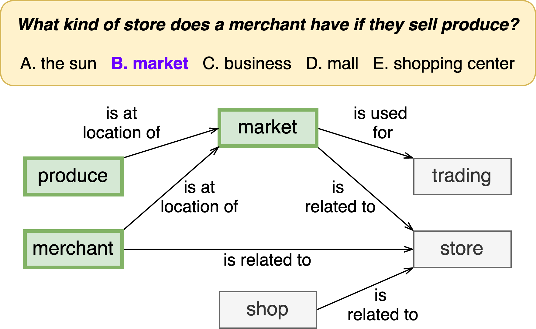
Figure 1: KG Saliency Explanations for Commonsense QA. Across different questions, the KG’s usefulness can vary considerably. Coarse explanations indicate if the KG is useful overall, while fine explanations highlight useful nodes or paths. Here, the fine explanations state that the market, produce, and merchant nodes are useful, while the other nodes are not.

In this paper, we investigate how saliency explanations can be used to improve KG-augmented models’ performance. First, we propose to create coarse (graph-level) and fine (node-/path-level) saliency explanations. Since KGs have features at different granularities, saliency explanations can supply a rich array of signals for learning to focus on useful KG features. To create coarse explanations, we introduce an ensemble-based saliency method which measures the performance difference between a KG-augmented model and its corresponding non-KG-augmented model. To create fine explanations, we can adapt any off-the-shelf saliency method, e.g., gradient-based [10] or occlusion-based [30]. Second, to demonstrate the potential of saliency-based supervision, we analyze the performance of oracle KG-augmented models, whose attention weights are directly masked with coarse and/or fine saliency explanations.

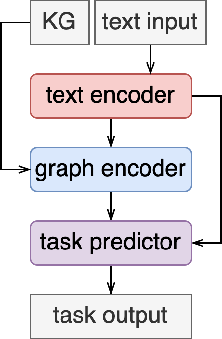
Figure 2: KG-Augmented Models fuse knowledge from text and KG inputs to solve CSR tasks.

Third, as motivated by our oracle model analysis, we propose the Learning from Saliency Explanations of KG-Augmented Models (SalKG) framework. Given coarse and/or fine explanations created from thse task’s training set, SalKG jointly trains the model to predict the explanations, then solve the task by attending to KG features highlighted in the predicted explanations. Using saliency explanations to regularize the attention mechanism can help the model generalize better to unseen instances, especially when coarse and fine explanations are used together as complementary learning signals. Indeed, on three standard commonsense QA benchmarks (CSQA, OBQA, CODAH) and a range of KG-augmented models, we show that SalKG can achieve considerable performance gains.

2 Preliminaries

Since KGs abundantly provide structured commonsense knowledge, KG-augmented models are often helpful for solving CSR tasks. CSR tasks are generally formulated as multi-choice QA (discriminative) tasks [52, 39, 23], but sometimes framed as open-ended response (generative) [33, 32] tasks. Given that multi-choice QA has been more extensively studied, we consider CSR in terms of multi-choice QA. Here, we present the multi-choice QA problem setting (Fig. 1) and the structure of KG-augmented models (Fig. 2).

Problem Definition  Given a question $q$ and set of answer choices $A=\{a_{i}\}$, a multi-choice QA model aims to predict a plausibility score $\rho(q,a_{i})$ for each $(q,a_{i})$ pair, so that the predicted answer $\hat{a}=\operatorname*{arg\,max}_{a_{i}\in A}\hskip 1.42262pt\rho(q,a_{i})$ matches the target answer $a^{*}$. Let $q\oplus a_{i}$ be the text statement formed from $(q,a_{i})$, where $\oplus$ denotes concatenation. For example, in Fig. 1, the text statement for $q\oplus a^{*}$ would be: What kind of store does a merchant have if they sell produce? market. We abbreviate $q\oplus a_{i}$ as $x_{i}$ and its plausibility score as $\rho(x_{i})$.

KG-Augmented Models  KG-augmented models use additional supervision from knowledge graphs to solve the multi-choice QA task. They encode the text and KG inputs individually as embeddings, then fuse the two embeddings together to use for prediction. A KG is denoted as $\tilde{\mathcal{G}}=(\tilde{\mathcal{V}},\tilde{\mathcal{R}},\tilde{\mathcal{E}})$, where $\tilde{\mathcal{V}}$, $\tilde{\mathcal{R}}$, and $\tilde{\mathcal{E}}$ are the KG’s nodes (concepts), relations, and edges (facts), respectively. An edge is a directed triple of the form $e=(c_{1},r,c_{2})\in\tilde{\mathcal{E}}$, in which $c_{1},c_{2}\in\tilde{\mathcal{V}}$ are nodes, and $r\in\tilde{\mathcal{R}}$ is the relation between $c_{1}$ and $c_{2}$. A path is a connected sequence of edges in the KG. When answering a question, the model does not use the entire KG, since most information in $\tilde{\mathcal{G}}$ is irrelevant to $x_{i}$. Instead, the model uses a smaller, contextualized KG $\mathcal{G}_{i}=(\mathcal{V}_{i},\mathcal{R}_{i},\mathcal{E}_{i})$, which is built from $\tilde{\mathcal{G}}$ using $x_{i}$. $\mathcal{G}_{i}$ can be constructed heuristically by extracting edges from $\tilde{\mathcal{G}}$ [31, 37], generating edges with a PLM [5], or both [56, 60]. In this paper, we consider KG-augmented models where $\mathcal{G}_{i}$ is built by heuristically by extracting edges from $\tilde{\mathcal{G}}$ (see Sec. A.1 for more details), since most KG-augmented models follow this paradigm. If $x_{i}$ and $\mathcal{G}_{i}$ are not discussed in the context of other answer choices, then we further simplify $x_{i}$’s and $\mathcal{G}_{i}$’s notation as $x$ and $\mathcal{G}$, respectively. Since the model never uses the full KG at once, we use “KG” to refer to $\mathcal{G}$ in the rest of the paper.

As in prior works [31, 5], a KG-augmented model $\mathcal{F}_{\text{KG}}$ has three main components: text encoder $f_{\text{text}}$, graph encoder $f_{\text{graph}}$, and task predictor $f_{\text{task}}$ (Fig. 2). Meanwhile, its corresponding non-KG-augmented model $\mathcal{F}_{\text{No-KG}}$ has no graph encoder but has a slightly different task predictor $\bar{f}_{\text{task}}$ which only takes $\mathbf{x}$ as input. In both $\mathcal{F}_{\text{KG}}$ and $\mathcal{F}_{\text{No-KG}}$, the task predictor outputs $\rho(x)$. Let $\mathbf{x}$ and $\mathbf{g}$ be the embeddings of $x$ and $\mathcal{G}$, respectively. Then, the workflows of $\mathcal{F}_{\text{KG}}$ and $\mathcal{F}_{\text{No-KG}}$ are defined below:

$$\mathbf{x}=f_{\text{text}}(x);\quad\mathbf{g}=f_{\text{graph}}(\mathcal{G},\mathbf{x});\quad\mathcal{F}_{\text{KG}}(x,\mathcal{G})=f_{\text{task}}(\mathbf{x}\oplus\mathbf{g});\quad\mathcal{F}_{\text{No-KG}}(x)=\bar{f}_{\text{task}}(\mathbf{x}).$$

Typically, $f_{\text{text}}$ is a PLM [11, 35], $f_{\text{graph}}$ is a graph neural network (GNN) [13, 47] or edge/path aggregation model [31, 5, 46], and $f_{\text{task}}$ and $\bar{f}_{\text{task}}$ are multilayer perceptrons (MLPs). In general, $f_{\text{graph}}$ reasons over $\mathcal{G}$ by encoding either nodes or paths, then using soft attention to pool the encoded nodes/paths into $\mathbf{g}$. Let $\mathcal{L}_{\text{task}}$ be the task loss for training $\mathcal{F}_{\text{KG}}$ and $\mathcal{F}_{\text{No-KG}}$. For multi-choice QA, $\mathcal{L}_{\text{task}}$ is cross-entropy loss, with respect to the distribution over $A$. For brevity, when comparing different models, we may also refer to $\mathcal{F}_{\text{KG}}$ and $\mathcal{F}_{\text{No-KG}}$ as KG and No-KG, respectively.

3 Creating KG Saliency Explanations

Explanation Setting	Unit
Coarse	KG
Fine (MHGRN)	Node
Fine (PathGen)	Path
Fine (RN)	Path

Table 1: KG unit types used for different explanation modes (Sec. 3) and graph encoders (Sec. 4.2).

Now, we show how to create coarse and fine saliency explanations, which tell us if the KG or certain parts of the KG are useful. These explanations can be used as extra inputs to mask oracle models’ attention (Sec. 4) or as extra supervision to regularize SalKG models’ attention (Sec. 5). We first abstractly define a unit as either $\mathcal{G}$ itself or a component of $\mathcal{G}$. A unit can be a graph, node, path, etc., and we categorize units as coarse (the entire graph $\mathcal{G}$) or fine (a node or path within $\mathcal{G}$) (Table 1). Given a model and task instance $(x,\mathcal{G})$, we define an explanation as a binary indicator of whether a unit $u$ of $\mathcal{G}$ is useful for the model’s prediction on $(x,\mathcal{G})$. If $u$ is useful, then $u$ should strongly influence the model to solve the instance correctly. By making explanations binary, we can easily use explanations as masks or learning targets (since binary labels are easier to predict than real-valued scores) for attention weights.

3.1 Coarse Saliency Explanations

Since $\mathcal{G}$ may not always be useful, a KG-augmented model should ideally know when to use $\mathcal{G}$. Here, the unit $u$ is the graph $\mathcal{G}$. Given instance $(x,\mathcal{G})$, a coarse saliency explanation $y_{\text{c}}(x,\mathcal{G})\in\{0,1\}$ indicates if $\mathcal{G}$ helps the model solve the instance. By default, $\mathcal{F}_{\text{KG}}$ assumes $\mathcal{G}$ is used, so we propose an ensemble-based saliency formulation for $y_{\text{c}}(x,\mathcal{G})$. That is, we define $y_{\text{c}}(x,\mathcal{G})$ as stating if $\mathcal{F}_{\text{KG}}$ (i.e., uses $\mathcal{G}$) or $\mathcal{F}_{\text{No-KG}}$ (i.e., does not use $\mathcal{G}$) should be used to solve $(x,\mathcal{G})$. Under this formulation, each $(x,\mathcal{G})$ has coarse units $\mathcal{G}$ and None, where None means “$\mathcal{G}$ is not used”.

To get $y_{\text{c}}(x,\mathcal{G})$, we begin by computing coarse saliency score $s_{\text{c}}(x,\mathcal{G})\in\mathbb{R}$, which we define as the performance difference between $\mathcal{F}_{\text{KG}}$ and $\mathcal{F}_{\text{No-KG}}$. For QA input $x_{i}=q\oplus a_{i}$ and its KG $\mathcal{G}_{i}$, let $p_{\text{KG}}(x_{i},\mathcal{G}_{i})$ and $p_{\text{No-KG}}(x_{i})$ be the confidence probabilities for $x_{i}$ predicted by $\mathcal{F}_{\text{KG}}$ and $\mathcal{F}_{\text{No-KG}}$, respectively.

$$s_{\text{c}} (x_{i},\mathcal{G}_{i})$$

$$= \begin{cases}p_{\text{KG}}(x_{i},\mathcal{G}_{i})-p_{\text{No-KG}}(x_{i}),&a_{i}=a^{*},\\ p_{\text{No-KG}}(x_{i})-p_{\text{KG}}(x_{i},\mathcal{G}_{i}),&a_{i}\neq a^{*}.\end{cases}$$ (1)

Ideally, a QA model should predict higher probabilities for answer choices $a_{i}$ that are correct, and vice versa. To capture this notion, we define $s_{\text{c}}(x_{i},\mathcal{G}_{i})$ in Eq. 1, where $a^{*}$ denotes the correct answer. Note that $s_{\text{c}}(x_{i},\mathcal{G}_{i})$ is positive if $p_{\text{KG}}(x_{i},\mathcal{G}_{i})$ is higher than $p_{\text{No-KG}}(x_{i})$ for correct choices and lower for incorrect choices. We obtain $y_{\text{c}}(x_{i},\mathcal{G}_{i})$ by binarizing $s_{\text{c}}(x_{i},\mathcal{G}_{i})$ to $0$ or $1$ based on whether it is greater than or less than a threshold $T$, respectively. If $y_{\text{c}}(x_{i},\mathcal{G}_{i})=1$, then the KG is useful, and vice versa. See the appendix for more details about why we use ensemble-based saliency for coarse explanations (Sec. A.2) and how we tune $T$ (Sec. A.6).

3.2 Fine Saliency Explanations

Even if $\mathcal{G}$ is useful, not every part of $\mathcal{G}$ may be useful. Hence, fine saliency explanations can identify which parts of a KG are actually useful. For a given instance $(x,\mathcal{G})$, we denote the fine saliency explanation for a fine unit $u$ in $\mathcal{G}$ as $y_{\text{f}}(u;x,\mathcal{G})\in\{0,1\}$. Fine units can be nodes, paths, etc. in the KG. If a graph encoder $f_{\text{graph}}$ encodes a certain type of unit, it is natural to define $y_{\text{f}}(u;x,\mathcal{G})$ with respect to such units. For example, MHGRN [13] encodes $\mathcal{G}$’s nodes, so we define MHGRN’s fine saliency explanations with respect to nodes. Similar to coarse saliency explanations, to obtain $y_{\text{f}}(u;x,\mathcal{G})$, we first compute fine saliency score $s_{\text{f}}(u;x,\mathcal{G})\in\mathbb{R}$, and then binarize it. For a QA input $x_{i}=q\oplus a_{i}$ and its KG $\mathcal{G}_{i}$, let $u_{ij}$ be the $j^{th}$ fine unit in $\mathcal{G}_{i}$ and $p_{\text{KG}}(x_{i},\mathcal{G}_{i})$ denote $\mathcal{F}_{\text{KG}}$’s predicted probability for $x_{i}$. There are many existing saliency methods (a.k.a. attribution methods) [10, 51, 30] for calculating the importance score of an input, with respect to a model and a given label. While $s_{\text{f}}(u_{ij};x_{i},\mathcal{G}_{i})$ can be computed via any saliency method, we use gradient-based and occlusion-based methods, since they are the most common types of saliency methods [2].

Let $\phi(u_{ij};x_{i},\mathcal{G}_{i})$ denote the raw saliency score given by some saliency method. Gradient-based methods measure an input’s saliency via the gradient of the model’s output with respect to the input. We use the gradient$\times$input (Grad) method [10], where $\phi(u_{ij};x_{i},\mathcal{G}_{i})$ is the dot product of $u_{ij}$’s embedding and the gradients of $p_{\text{KG}}(x_{i},\mathcal{G}_{i})$ with respect to $u_{ij}$. Occlusion-based methods measure an input’s saliency as how the model’s output is affected by erasing that input. We use the leave-one-out (Occl) method [30], where $\phi(u_{ij};x_{i},\mathcal{G}_{i})$ is the decrease in $p_{\text{KG}}(x_{i},\mathcal{G}_{i})$ if $u_{ij}$ is removed from $\mathcal{G}_{i}$, i.e., $\phi(u_{ij};x_{i},\mathcal{G}_{i})$ = $p_{\text{KG}}(x_{i},\mathcal{G}_{i})$ - $p_{\text{KG}}(x_{i},\mathcal{G}_{i}\setminus u_{ij})$.

$$s_{\text{f}} (u_{ij};x_{i},\mathcal{G}_{i})$$

$$= \begin{cases}\phi(u_{ij};x_{i},\mathcal{G}_{i}),&a_{i}=a^{*}\\ -\phi(u_{ij};x_{i},\mathcal{G}_{i}),&a_{i}\neq a^{*}\end{cases}$$ (2)

Intuitively, a unit is more useful if it increases the probability of correct answer choice $a^{*}$, and vice versa. Thus, we define the saliency score $s_{\text{f}}(u_{ij};x_{i},\mathcal{G}_{i})$ for unit $u_{ij}$ as Eq. 2. Next, we binarize the saliency scores to get $y_{\text{f}}(u_{ij};x_{i},\mathcal{G}_{i})$, by selecting the top-$k$%-scoring units in $\mathcal{G}_{i}$ and setting $y_{\text{f}}(u_{ij};x_{i},\mathcal{G}_{i})=1$ (i.e., $u_{ij}$ is useful) for these units. For all other units in $\mathcal{G}$, we set $y_{\text{f}}(u_{ij};x_{i},\mathcal{G}_{i})=0$ (i.e., $u_{ij}$ is not useful). See the appendix for more details about the fine saliency methods (Sec. A.3) and tuning threshold $k$ (Sec. A.6).

4 Oracle: Using KG Saliency Explanations as Inputs

In this section, we analyze KG saliency explanations’ potential to improve KG-augmented models’ performance. Recall that creating saliency explanations requires the task’s ground truth labels (Sec. 3), so directly using test set explanations is infeasible. Still, before exploring ways to leverage training set explanations (Sec. 5), we first establish upper bounds on how much models can benefit from saliency explanations. Here, we study three key questions: (1) Does the model improve when provided oracle access to coarse/fine explanations? (2) Are coarse and fine explanations complementary? (3) How do gradient-based explanations compare to occlusion-based explanations?

4.1 Oracle Models

Oracle models are KG-augmented models with oracle access to saliency explanations. An Oracle model uses ground truth labels to create explanations (even at inference time), and then uses the explanations as extra inputs to perform hard attention over the units. We define the model attention weights that are modified based on saliency explanations as saliency weights. Below, we introduce the Oracle-Coarse, Oracle-Fine, and Oracle-Hybrid models, shown in Fig. 3a-c.

Oracle-Coarse  Oracle-Coarse ($\mathcal{F}_{\text{c}}^{*}$) uses coarse explanations to do hard attention over $\mathcal{F}_{\text{KG}}$’s and $\mathcal{F}_{\text{No-KG}}$’s predictions. First, $\mathcal{F}_{\text{KG}}$ and $\mathcal{F}_{\text{No-KG}}$ are trained separately, then frozen. Next, for each instance $(x,\mathcal{G})$, they are used to create a coarse explanation $y_{\text{c}}(x,\mathcal{G})\in\{0,1\}$. Then, $\mathcal{F}_{\text{c}}^{*}$ is defined as an ensemble model that performs hard attention over coarse units ($\mathcal{G}$ and None) by weighting $\mathcal{F}_{\text{KG}}$’s prediction with $y_{\text{c}}(x,\mathcal{G})$ and $\mathcal{F}_{\text{No-KG}}$’s prediction with $1-y_{\text{c}}(x,\mathcal{G})$ (Table 2; Fig. 3a). In other words, $y_{\text{c}}(x,\mathcal{G})$ and $1-y_{\text{c}}(x,\mathcal{G})$ are the saliency weights for $\mathcal{F}_{\text{c}}^{*}$.

Oracle-Fine  Oracle-Fine ($\mathcal{F}_{\text{f}}^{*}$) has the same architecture as $\mathcal{F}_{\text{KG}}$ and uses fine explanations to do hard attention over fine units (i.e., nodes or paths in $\mathcal{G}$). First, $\mathcal{F}_{\text{KG}}$ is trained, then frozen. As usual, $\mathcal{F}_{\text{KG}}$ uses soft attention over fine units in $\mathcal{G}$ to compute graph embedding $\mathbf{g}$ (Sec. 2). Then, for each fine unit $u$ in $\mathcal{G}$, $\mathcal{F}_{\text{KG}}$ is used to create fine explanation $y_{\text{f}}(u;x,\mathcal{G})\in\{0,1\}$. Let $\hat{y}_{\text{f}}(u;x,\mathcal{G})\in[0,1]$ denote $\mathcal{F}_{\text{f}}^{*}$’s soft attention weight for $u$. We train $\mathcal{F}_{\text{f}}^{*}$ the same way as $\mathcal{F}_{\text{KG}}$, except each $\hat{y}_{\text{f}}(u;x,\mathcal{G})$ is (hard attention) masked with $y_{\text{f}}(u;x,\mathcal{G})$, i.e., $\hat{y}_{\text{f}}(u;x,\mathcal{G})\leftarrow\hat{y}_{\text{f}}(u;x,\mathcal{G})\odot y_{\text{f}}(u;x,\mathcal{G})$, where $\odot$ denotes element-wise multiplication (Table 2; Fig. 3b). This means only units with $y_{\text{f}}(u;x,\mathcal{G})=1$ will have $\hat{y}_{\text{f}}(u;x,\mathcal{G})>0$ and thus be able to influence $\mathcal{F}_{\text{f}}^{*}$’s prediction. Let $y_{\text{f}}(x,\mathcal{G})$ and $\hat{y}_{\text{f}}(x,\mathcal{G})$ denote the explanations and soft attention weights, respectively, for all units in the graph. Then, $\hat{y}_{\text{f}}(x,\mathcal{G})\odot y_{\text{f}}(x,\mathcal{G})$ are the saliency weights for $\mathcal{F}_{\text{f}}^{*}$.

Oracle-Hybrid  Oracle-Hybrid ($\mathcal{F}_{\text{h}}^{*}$) unifies Oracle-Coarse and Oracle-Fine as a single model, thus leveraging the coarse-fine hierarchy inherent in KG saliency explanations. First, $\mathcal{F}_{\text{f}}^{*}$ (which uses fine explanations) and $\mathcal{F}_{\text{No-KG}}$ are separately trained, then frozen. Then, for each $(x,\mathcal{G})$, $\mathcal{F}_{\text{f}}^{*}$ and $\mathcal{F}_{\text{No-KG}}$ are used to create $y_{\text{h}}(x,\mathcal{G})\in\{0,1\}$, which we define as the coarse explanation for $\mathcal{F}_{\text{f}}^{*}$ and $\mathcal{F}_{\text{No-KG}}$. $y_{\text{h}}(x,\mathcal{G})$ is computed the same way as $y_{\text{c}}(x,\mathcal{G})$, besides replacing $\mathcal{F}_{\text{KG}}$ with $\mathcal{F}_{\text{f}}^{*}$. Finally, similar to $\mathcal{F}_{\text{c}}^{*}$, $\mathcal{F}_{\text{h}}^{*}$ is an ensemble that performs hard attention over coarse units by weighting $\mathcal{F}_{\text{f}}^{*}$’s prediction with $y_{\text{h}}(x,\mathcal{G})$ and $\mathcal{F}_{\text{No-KG}}$’s prediction with $1-y_{\text{h}}(x,\mathcal{G})$ (Table 2; Fig. 3c). That is, $y_{\text{h}}(x,\mathcal{G})$ and $1-y_{\text{h}}(x,\mathcal{G})$ are the saliency weights for $\mathcal{F}_{\text{h}}^{*}$.

Model	Output	Saliency Weights
Oracle-Coarse	$\mathcal{F}_{\text{c}}^{*}(x,\mathcal{G})=y_{\text{c}}(x,\mathcal{G})\mathcal{F}_{\text{KG}}(x,\mathcal{G})+(1-y_{\text{c}}(x,\mathcal{G}))\mathcal{F}_{\text{No-KG}}(x)$	$[y_{\text{c}}(x,\mathcal{G}),1-y_{\text{c}}(x,\mathcal{G})]$
Oracle-Fine	$\mathcal{F}_{\text{f}}^{*}(x,\mathcal{G})\sim\mathcal{F}_{\text{KG}}(x,\mathcal{G})$	$\hat{y}_{\text{f}}(x,\mathcal{G})\odot y_{\text{f}}(x,\mathcal{G})$
Oracle-Hybrid	$\mathcal{F}_{\text{h}}^{*}(x,\mathcal{G})=y_{\text{h}}(x,\mathcal{G})\mathcal{F}_{\text{f}}^{*}(x,\mathcal{G})+(1-y_{\text{h}}(x,\mathcal{G}))\mathcal{F}_{\text{No-KG}}(x)$	$[y_{\text{h}}(x,\mathcal{G}),1-y_{\text{h}}(x,\mathcal{G})]$

Table 2: Comparison of Oracle Models. For each Oracle Model, we show its output and saliency weights. Note that the explanations are given (not predicted), so there is no $\mathcal{L}_{\text{sal}}$. While $\mathcal{F}_{\text{c}}^{*}$ and $\mathcal{F}_{\text{h}}^{*}$ are both ensembles of $\mathcal{F}_{\text{KG}}$ and $\mathcal{F}_{\text{No-KG}}$, $\mathcal{F}_{\text{f}}^{*}$ has the same architecture as $\mathcal{F}_{\text{KG}}$ (denoted by $\sim$) besides the attention masking.

4.2 Evaluation Protocol

We use the CSQA [52] and OBQA [39] multi-choice QA datasets. For CSQA, we use the accepted in-house data split from [31], as the official test labels are not public. As in prior works, we use the ConceptNet [49] KG for both datasets. We report accuracy, the standard metric for multi-choice QA. For $\mathcal{F}_{\text{No-KG}}$ and $\mathcal{F}_{\text{KG}}$, we pick the best model over three seeds, then use them to create explanations for Oracle models. We use thresholds $T=0.01$ and $k=10$ for coarse and fine explanations, respectively. For text encoders, we use BERT(-Base) [11] and RoBERTa(-Large) [35]. For graph encoders, we use MHGRN [13], PathGen [56], and Relation Network (RN) [46, 31]. MHGRN has node units, while PathGen and RN have path units. As baseline models, we use $\mathcal{F}_{\text{No-KG}}$, $\mathcal{F}_{\text{KG}}$, and $\mathcal{F}_{\text{No-KG}}+\mathcal{F}_{\text{KG}}$, where $\mathcal{F}_{\text{No-KG}}+\mathcal{F}_{\text{KG}}$ is an ensemble whose prediction is the mean of $\mathcal{F}_{\text{No-KG}}$’s and $\mathcal{F}_{\text{KG}}$’s predictions. Oracle and baseline models are trained only with task loss $\mathcal{L}_{\text{task}}$.

	CSQA Test Accuracy (%)						OBQA Test Accuracy (%)
	MHGRN		PathGen		RN		MHGRN		PathGen		RN
Model	BERT	RoBERTa	BERT	RoBERTa	BERT	RoBERTa	BERT	RoBERTa	BERT	RoBERTa	BERT	RoBERTa
No-KG	55.44	70.59	55.44	70.59	55.44	70.59	53.60	68.40	53.60	68.40	53.60	68.40
KG	56.57	73.33	56.65	72.04	55.60	71.07	53.20	69.80	55.00	67.80	58.60	70.20
No-KG + KG	56.57	71.39	57.45	73.00	56.73	68.49	55.60	70.60	54.40	70.6	53.40	69.60
Oracle-Coarse	66.16	81.39	68.57	80.10	67.28	79.69	70.60	79.40	65.00	76.60	69.00	79.00
Oracle-Fine (Grad)	74.86	76.15	79.61	87.35	81.39	83.24	67.60	72.60	73.80	73.40	68.00	62.80
Oracle-Fine (Occl)	91.06	87.99	79.61	75.34	73.73	68.41	77.00	71.20	83.60	62.60	55.60	61.40
Oracle-Hybrid (Grad)	85.50	84.21	90.49	92.83	92.26	93.56	80.80	84.80	85.60	92.80	85.40	86.80
Oracle-Hybrid (Occl)	95.89	98.63	88.96	96.78	85.25	95.25	87.00	89.60	92.80	90.60	67.40	80.60

Table 3: Oracle Performance on CSQA and OBQA

4.3 Analysis

In Table 3, we show CSQA and OBQA performance for the baseline and Oracle models. We analyze these results via the three questions below.

Does the model improve when provided oracle access to coarse/fine explanations?  Yes. Oracle-Coarse beats all baselines, while Oracle-Fine beats all baselines except on OBQA RN+RoBERTa. These results motivate us to develop a framework for models to improve performance by learning from coarse/fine explanations. Also, on average, Oracle-Fine outperforms Oracle-Coarse, which suggests that fine explanations may often provide richer signal than their coarse counterparts. Indeed, fine explanations indicate the saliency of every unit in the KG, while coarse explanations only indicate the saliency of the KG as a whole.

Are coarse and fine explanations complementary?  Yes. Across all settings, Oracle-Hybrid performs significantly better than Oracle-Coarse and Oracle-Fine. This suggests that coarse and fine explanations are complementary and that it is effective to leverage both hierarchically.

How do gradient-based explanations compare to occlusion-based explanations?  Overall, Grad and Occl perform similarly. Grad performs better on some settings (e.g., MHGRN), while Occl performs better on others (e.g., RN). See Table 8 and Sec. A.9 for more Grad vs. Occl experiments.

In our Oracle pilot study, KG-augmented models achieve large performance gains when given explanations as input. This suggests that, if oracle explanations can somehow be predicted accurately during inference without using ground truth labels, then KG-augmented models can still achieve improvements without directly using explanations as input. This motivates us to train KG-augmented models with explanation-based supervision via SalKG, which we describe in Sec. 5.

5 SalKG: Using KG Saliency Explanations as Supervision

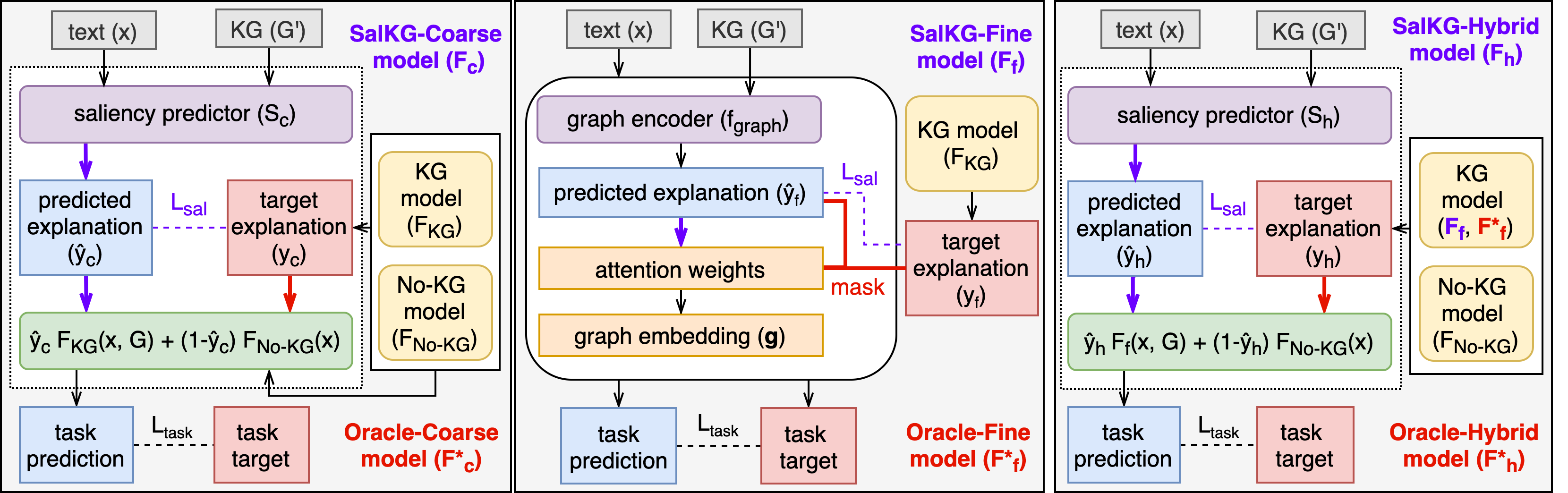
Figure 3: Schematics for Oracle and SalKG Models. Red arrows indicate the Oracle pipeline, where the target explanation is provided as input. Purple arrows indicate the SalKG pipeline, where the target explanation is used as supervision for the predicted explanation. In SalKG-Coarse and SalKG-Hybrid, the saliency predictor has the same architecture as $\mathcal{F}_{\text{KG}}$. Meanwhile, Oracle-Fine and SalKG-Fine (shown as white module, with text encoder and task predictor omitted) both have the same architecture as $\mathcal{F}_{\text{KG}}$.

Based on the analysis from Sec. 4.3, we propose the SalKG framework for KG-augmented models to learn from coarse/fine saliency explanations. Whereas Oracle models (Sec. 4.1) use explanations directly as extra inputs, SalKG models only use them as extra supervision during the training phase. With explanations created from the training set via $\mathcal{F}_{\text{KG}}$ and $\mathcal{F}_{\text{No-KG}}$, SalKG models are jointly trained to predict the explanations (via saliency loss $\mathcal{L}_{\text{sal}}$) and use the predicted explanations to solve the task (via task loss $\mathcal{L}_{\text{task}}$). Thus, SalKG models have the following objective: $\mathcal{L}_{\text{S}}=\mathcal{L}_{\text{task}}+\lambda\mathcal{L}_{\text{sal}}$, where $\lambda\geq 0$ is a loss weighting parameter. This multitask objective not only encourages SalKG models to focus on useful KG units for solving the task, but also to learn more general graph/node/path representations. Below, we present SalKG-Coarse, SalKG-Fine, and SalKG-Hybrid models.

SalKG-Coarse  Unlike Oracle-Coarse, SalKG-Coarse ($\mathcal{F}_{\text{c}}$) is not given oracle coarse explanation $y_{\text{c}}(x,\mathcal{G})$ as input. Instead, a saliency predictor $\mathcal{S}_{\text{c}}$ (with the same architecture as $\mathcal{F}_{\text{KG}}$) is trained to predict the oracle coarse explanation. $\mathcal{S}_{\text{c}}$ predicts coarse explanation as probability $\hat{y}_{\text{c}}(x,\mathcal{G})\in[0,1]$. $\mathcal{F}_{\text{c}}$’s output is an ensemble that does soft attention over coarse units by weighting $\mathcal{F}_{\text{KG}}$’s and $\mathcal{F}_{\text{No-KG}}$’s predictions with saliency weights $\hat{y}_{\text{c}}(x,\mathcal{G})$ and $1-\hat{y}_{\text{c}}(x,\mathcal{G})$, respectively (Table 4; Fig. 3a). Here, $\mathcal{L}_{\text{sal}}(\hat{y}_{\text{c}}(x,\mathcal{G}),y_{\text{c}}(x,\mathcal{G}))$ is the cross-entropy loss.

SalKG-Fine  Similarly, SalKG-Fine ($\mathcal{F}_{\text{f}}$) is not given oracle fine explanation $y_{\text{f}}(u;x,\mathcal{G})$ as input, although both have the same architecture as $\mathcal{F}_{\text{KG}}$. Instead, for each fine unit $u$, $\mathcal{F}_{\text{f}}$’s attention mechanism is trained to predict $y_{\text{f}}(u;x,\mathcal{G})$ as soft attention weight $\hat{y}_{\text{f}}(u;x,\mathcal{G})\in[0,1]$ (Table 4; Fig. 3b). As before, $\hat{y}_{\text{f}}(x,\mathcal{G})=[\hat{y}_{\text{f}}(u;x,\mathcal{G})]_{u\in\mathcal{G}}$ are the soft attention weights for $(x,\mathcal{G})$, while $y_{\text{f}}(x,\mathcal{G})=[y_{\text{f}}(u;x,\mathcal{G})]_{u\in\mathcal{G}}$ are the fine explanations for $(x,\mathcal{G})$. Then, $\hat{y}_{\text{f}}(x,\mathcal{G})$ are the saliency weights for $\mathcal{F}_{\text{f}}$, trained with KL divergence loss $\mathcal{L}_{\text{sal}}(\hat{y}_{\text{f}}(x,\mathcal{G}),y_{\text{f}}(x,\mathcal{G}))$.

SalKG-Hybrid  Similar to the other SalKG variants, SalKG-Hybrid ($\mathcal{F}_{\text{h}}$) does not use any oracle explanations. Like in SalKG-Coarse, a saliency predictor $\mathcal{S}_{\text{h}}$ is trained to predict oracle coarse explanation $y_{h}(x,\mathcal{G})$ (Sec. 4.1). Predicted coarse explanation probabilities $\hat{y}_{\text{h}}(x,\mathcal{G})\in[0,1]$ are then used as soft attention over coarse units by weighting $\mathcal{F}_{\text{f}}$’s and $\mathcal{F}_{\text{No-KG}}$’s predictions with weights $\hat{y}_{\text{h}}(x,\mathcal{G})$ and $1-\hat{y}_{\text{h}}(x,\mathcal{G})$, respectively (Table 4; Fig. 3c). Here, $\mathcal{L}_{\text{sal}}(\hat{y}_{\text{h}}(x,\mathcal{G}),y_{\text{h}}(x,\mathcal{G}))$ is cross-entropy loss.

Model	Output	Saliency Weights	Saliency Loss ($\mathcal{L}_{\text{sal}}$)
SalKG-Coarse	$\mathcal{F}_{\text{c}}(x,\mathcal{G})=\hat{y}_{\text{c}}(x,\mathcal{G})\hskip 1.42262pt\mathcal{F}_{\text{KG}}(x,\mathcal{G})+(1-\hat{y}_{\text{c}}(x,\mathcal{G}))\hskip 1.42262pt\mathcal{F}_{\text{No-KG}}(x)$	$[\hat{y}_{\text{c}}(x,\mathcal{G}),1-\hat{y}_{\text{c}}(x,\mathcal{G})]$	CE$(\hat{y}_{\text{c}}(x,\mathcal{G}),y_{\text{c}}(x,\mathcal{G}))$
SalKG-Fine	$\mathcal{F}_{\text{f}}(x,\mathcal{G})\sim\mathcal{F}_{\text{KG}}(x,\mathcal{G})$	$\hat{y}_{\text{f}}(x,\mathcal{G})$	KL$(\hat{y}_{\text{f}}(x,\mathcal{G}),y_{\text{f}}(x,\mathcal{G}))$
SalKG-Hybrid	$\mathcal{F}_{\text{h}}(x,\mathcal{G})=\hat{y}_{\text{h}}(x,\mathcal{G})\mathcal{F}_{\text{f}}(x,\mathcal{G})+(1-\hat{y}_{\text{h}}(x,\mathcal{G}))\mathcal{F}_{\text{No-KG}}(x)$	$[\hat{y}_{\text{h}}(x,\mathcal{G}),1-\hat{y}_{\text{h}}(x,\mathcal{G})]$	CE$(\hat{y}_{\text{h}}(x,\mathcal{G}),y_{\text{h}}(x,\mathcal{G}))$

Table 4: Comparison of SalKG Models. For each SalKG Model, we show its output, saliency weights, and $\mathcal{L}_{\text{sal}}$. While $\mathcal{F}_{\text{c}}$ and $\mathcal{F}_{\text{h}}$ are both ensembles, $\mathcal{F}_{\text{f}}$ has the same architecture as $\mathcal{F}_{\text{KG}}$ (denoted by $\sim$). “CE” denotes cross-entropy loss, while “KL” denotes KL divergence loss.

6 Experiments

6.1 Evaluation Protocol

We evaluate SalKG models on the CSQA [52], OBQA [39], and CODAH [6] multi-choice QA datasets (Sec. A.5). In addition to the baselines in Sec. 4.2, we consider two new baselines, Random and Heuristic, which help show that coarse/fine saliency explanations provide strong learning signal for KG-augmented models to focus on useful KG features. We follow the same evaluation protocol in Sec. 4.2, except we now also report mean and standard deviation performance over multiple seeds. See Sec. A.4 for a more detailed description of the evaluation protocol.

Random  Random is a variant of SalKG where each unit’s explanation is random. Random-Coarse is like SalKG-Coarse, but with each $y_{\text{c}}(x,\mathcal{G})$ uniformly sampled from $\{0,1\}$. Random-Fine is like SalKG-Fine, but randomly picking $k$% of units in $\mathcal{G}$ to set $y_{\text{f}}(u;x,\mathcal{G})=1$. Random-Hybrid is like SalKG-Hybrid, but with each $y_{\text{h}}(x,\mathcal{G})$ uniformly sampled from $\{0,1\}$ as well as using Random-Fine instead of SalKG-Fine.

Heuristic  Each $\mathcal{G}$ has three node types: question nodes (i.e., nodes in $q$), answer nodes (i.e., nodes in $a_{i}$), and intermediate nodes (i.e., other nodes) [31]. Let QA nodes be nodes in $q$ or $a_{i}$. Heuristic is a variant of SalKG where each unit’s explanation is based on the presence of QA nodes in $\mathcal{G}$. Let $\bar{N}$ be the mean number of QA nodes per KG (in train set), and let $N(\mathcal{G})$ be the number of QA nodes in $\mathcal{G}$. Heuristic-Coarse is like SalKG-Coarse, except $y_{\text{c}}(x,\mathcal{G})=1$ if and only if $N(\mathcal{G})>\bar{N}$. Heuristic-Fine is like SalKG-Fine, but how $y_{\text{f}}(u;x,\mathcal{G})$ is set depends on whether the fine units are nodes or paths. For node units, $y_{\text{f}}(u;x,\mathcal{G})=1$ if and only if $u$ is a QA node. For path units, $y_{\text{f}}(u;x,\mathcal{G})=1$ if and only if $u$ consists only of QA nodes. Heuristic-Hybrid is like SalKG-Hybrid, but with $y_{\text{h}}(x,\mathcal{G})=1$ if and only if $N(\mathcal{G})>\bar{N}$, while Heuristic-Fine is used instead of SalKG-Fine.

6.2 Main Results

Table 5 shows performance on CSQA, while Table 6 shows performance on OBQA and CODAH. Best performance is highlighted in green, second-best performance is highlighted in blue, and best non-SalKG performance is highlighted in red (if it is not already green or blue). For SalKG (unlike Oracle), we find that Occl usually outperforms Grad, so we only report Occl performance in Tables 5-6. For a comparison of Grad and Occl on SalKG, see Table 8 and Sec. A.9. Being an ensemble, No-KG + KG tends to beat both No-KG and KG if both have similar performance. Otherwise, No-KG + KG’s performance is in between No-KG’s and KG’s.

	CSQA Test Accuracy (%)
	MHGRN		PathGen		RN
Model	BERT	RoBERTa	BERT	RoBERTa	BERT	RoBERTa
No-KG	53.13 ($\pm$2.34)	69.65 ($\pm$1.06)	53.13 ($\pm$2.34)	69.65 ($\pm$1.06)	53.13 ($\pm$2.34)	69.65 ($\pm$1.06)
KG	57.48 ($\pm$0.89)	73.14 ($\pm$0.78)	56.54 ($\pm$0.73)	72.58 ($\pm$0.57)	56.46 ($\pm$1.22)	71.37 ($\pm$1.20)
No-KG + KG	56.14 ($\pm$2.28)	72.15 ($\pm$0.67)	57.29 ($\pm$1.30)	72.44 ($\pm$0.72)	55.98 ($\pm$1.98)	71.15 ($\pm$0.81)
Random-Coarse	55.04 ($\pm$1.44)	71.06 ($\pm$1.09)	55.09 ($\pm$1.08)	71.15 ($\pm$1.06)	55.15 ($\pm$1.23)	69.06 ($\pm$2.96)
Random-Fine	54.69 ($\pm$2.54)	73.09 ($\pm$1.06)	54.66 ($\pm$0.97)	71.26 ($\pm$3.19)	49.88 ($\pm$1.75)	69.08 ($\pm$1.95)
Random-Hybrid	52.43 ($\pm$2.60)	71.93 ($\pm$0.77)	55.24 ($\pm$0.58)	71.35 ($\pm$0.34)	54.36 ($\pm$0.35)	70.12 ($\pm$0.35)
Heuristic-Coarse	55.55 ($\pm$2.29)	72.15 ($\pm$0.84)	56.92 ($\pm$0.18)	72.57 ($\pm$0.49)	56.42 ($\pm$1.11)	71.18 ($\pm$0.77)
Heuristic-Fine	52.54 ($\pm$1.67)	71.50 ($\pm$1.01)	54.00 ($\pm$1.89)	71.11 ($\pm$0.93)	52.04 ($\pm$2.13)	65.08 ($\pm$3.67)
Heuristic-Hybrid	56.35 ($\pm$0.81)	72.58 ($\pm$0.32)	56.83 ($\pm$0.48)	71.33 ($\pm$0.87)	54.38 ($\pm$3.30)	65.07 ($\pm$2.02)
SalKG-Coarse	57.98 ($\pm$0.90)	73.64 ($\pm$1.05)	57.75 ($\pm$0.77)	73.07 ($\pm$0.25)	57.50 ($\pm$1.25)	73.11 ($\pm$1.13)
SalKG-Fine	54.36 ($\pm$2.34)	70.00 ($\pm$0.81)	54.39 ($\pm$2.03)	72.12 ($\pm$0.91)	54.30 ($\pm$1.41)	71.64 ($\pm$1.51)
SalKG-Hybrid	58.70 ($\pm$0.65)	73.37 ($\pm$0.12)	59.87 ($\pm$0.42)	72.67 ($\pm$0.65)	58.78 ($\pm$0.14)	74.13 ($\pm$0.71)

Table 5: SalKG Performance on CSQA

Across all datasets, we find that SalKG-Hybrid and SalKG-Coarse are consistently the two best models. On CSQA, SalKG-Hybrid has the highest performance on BERT+MHGRN, BERT+PathGen, BERT+RN, and RoBERTa+RN, while SalKG-Coarse is the best on RoBERTa+MHGRN and RoBERTa+PathGen. In particular, on RoBERTa+RN, BERT+RN, and BERT+PathGen, SalKG-Hybrid beats $\max$(No-KG, KG, No-KG + KG) by large margins of 2.76%, 2.58%, and 2.32%, respectively. Meanwhile, OBQA and CODAH, SalKG is not as dominant but still yields improvements overall. On OBQA, SalKG-Coarse is the best on RoBERTa+RN (beating $\max$(No-KG, KG, No-KG + KG) by 1.89%) and RoBERTa+PathGen, while SalKG-Hybrid performs best on RoBERTa+MHGRN. On CODAH, SalKG-Coarse gets the best performance on both RoBERTa+MHGRN (beating $\max$(No-KG, KG, No-KG + KG) by 1.71%) and RoBERTa+PathGen. SalKG-Coarse outperforming SalKG-Hybrid on OBQA and CODAH indicates that local KG supervision from fine explanations may not be as useful for these two datasets. On the other hand, SalKG-Fine is consistently weaker than SalKG-Hybrid and SalKG-Coarse, but still shows slight improvement for RoBERTa+RN on CSQA. These results show that learning from KG saliency explanations is generally effective for improving KG-augmented models’ performance, especially in CSQA when both coarse and fine explanations are used to provide complementary learning signals for SalKG-Hybrid. Furthermore, across all datasets, we find that SalKG outperforms Random and Heuristic on every setting. This is evidence that explanations created from saliency methods can provide better learning signal than those created randomly or from simple heuristics.

	OBQA Test Accuracy (%)			CODAH Test Accuracy (%)
Model (RoBERTa)	MHGRN	PathGen	RN	MHGRN	PathGen
No-KG	68.73 ($\pm$0.31)	68.73 ($\pm$0.31)	68.73 ($\pm$0.31)	83.96 ($\pm$0.79)	83.96 ($\pm$0.79)
KG	68.87 ($\pm$2.16)	68.40 ($\pm$1.59)	66.80 ($\pm$4.73)	84.02 ($\pm$1.27)	84.02 ($\pm$1.62)
No-KG + KG	68.53 ($\pm$0.95)	69.67 ($\pm$1.45)	69.40 ($\pm$0.35)	84.08 ($\pm$1.46)	84.69 ($\pm$1.48)
Random-Coarse	68.11 ($\pm$1.12)	67.18 ($\pm$4.13)	65.02 ($\pm$2.57)	83.48 ($\pm$0.91)	84.68 ($\pm$1.65)
Random-Fine	57.60 ($\pm$5.33)	55.13 ($\pm$7.00)	48.53 ($\pm$4.82)	74.77 ($\pm$6.90)	80.48 ($\pm$1.23)
Random-Hybrid	68.33 ($\pm$0.40)	69.53 ($\pm$0.31)	69.27 ($\pm$0.12)	83.86 ($\pm$0.69)	83.75 ($\pm$0.60)
Heuristic-Coarse	69.24 ($\pm$2.47)	65.58 ($\pm$6.08)	64.29 ($\pm$3.06)	82.64 ($\pm$0.10)	82.52 ($\pm$0.18)
Heuristic-Fine	57.27 ($\pm$3.76)	51.80 ($\pm$2.95)	50.53 ($\pm$3.51)	82.25 ($\pm$1.43)	82.55 ($\pm$2.03)
Heuristic-Hybrid	68.47 ($\pm$0.23)	68.40 ($\pm$0.00)	68.60 ($\pm$0.20)	82.16 ($\pm$2.11)	82.73 ($\pm$1.51)
SalKG-Coarse	69.93 ($\pm$0.56)	70.02 ($\pm$0.55)	71.29 ($\pm$0.57)	85.79 ($\pm$1.83)	85.43 ($\pm$1.88)
SalKG-Fine	64.82 ($\pm$0.97)	51.51 ($\pm$0.87)	62.29 ($\pm$0.85)	84.08 ($\pm$1.14)	83.36 ($\pm$0.81)
SalKG-Hybrid	70.20 ($\pm$0.69)	69.80 ($\pm$0.49)	70.47 ($\pm$0.91)	85.17 ($\pm$0.54)	84.42 ($\pm$0.64)

Table 6: SalKG Performance on OBQA and CODAH

Model (RoBERTa)	CSQA Test Accuracy (%)
RN [46]	70.08 ($\pm$0.21)
RN + Link Prediction [56]	69.33 ($\pm$0.98)
RGCN [47]	68.41 ($\pm$0.66)
GAT [55]	71.20 ($\pm$0.72)
GN [4]	71.12 ($\pm$0.45)
GconAttn [57]	69.88 ($\pm$0.47)
MHGRN [13]	71.11 ($\pm$0.81)
PathGen [56]	72.68 ($\pm$0.42)
SalKG-Coarse (MHGRN)	74.01 ($\pm$0.14)
SalKG-Fine (MHGRN)	72.68 ($\pm$1.46)
SalKG-Hybrid (MHGRN)	73.87 ($\pm$0.48)
SalKG-Coarse (PathGen)	72.76 ($\pm$0.12)
SalKG-Fine (PathGen)	71.21 ($\pm$1.31)
SalKG-Hybrid (PathGen)	73.03 ($\pm$0.84)

Table 7: Comparison of SalKG to Published CSQA Baselines. SalKG models that outperform all baselines are shown in bold.

Comparison to Published CSQA Baselines

To further demonstrate that SalKG models perform competitively, we also compare SalKG (using MHGRN and PathGen) to the many KG-augmented model baseline results published in [13, 56, 60], for the CSQA in-house split. The baselines we consider are RN [46], RN + Link Prediction [13], RGCN [47], GAT [55], GN [4], GconAttn [57], MHGRN [13], and PathGen [56]. For the non-SalKG versions of MHGRN, PathGen, and RN, we quote the published results. Since these published results average over four seeds (instead of three), we report SalKG results over four seeds in Table 7. We find that most of the listed SalKG variants can outperform all of the baselines. For MHGRN, SalKG-Coarse (MHGRN) performs the best overall, SalKG-Hybrid (MHGRN) beats vanilla MHGRN, and SalKG-Fine (MHGRN) is on par with vanilla MHGRN. For PathGen, SalKG-Hybrid (PathGen) and SalKG-Coarse (PathGen) both slightly outperform vanilla PathGen, while SalKG-Fine (PathGen) performs worse.

CSQA Leaderboard Submission

In addition to our experiments on the CSQA in-house split, we evaluated SalKG on the CSQA official split by submitting SalKG to the CSQA leaderboard. Since the best models on the CSQA leaderboard use the ALBERT [24] text encoder, and PathGen was the highest graph encoder on the leaderboard out of the three we experimented with, we trained SalKG-Hybrid (ALBERT+PathGen), which achieved a test accuracy of 75.9%. For reference, a previously submitted ALBERT+PathGen achieved a test accuracy of 75.6% on the CSQA leaderboard. This result suggests that the proposed SalKG training procedure can yield some improvements over baselines that do not use explanation-based regularization.

Why does SalKG-Fine perform poorly?

In general, SalKG-Fine does not perform as well as SalKG-Coarse and SalKG-Hybrid. Often, SalKG-Fine is noticeably worse than KG and No-KG. Recall that the KG model and SalKG-Fine model both assume that the KG should always be used to solve the given instance. Still, the success of SalKG-Coarse shows that the KG sometimes may not be useful. But why does SalKG-Fine almost always perform worse than the KG model?

We believe it is because SalKG-Fine is more committed to the flawed assumption of universal KG usefulness. Whereas the KG model is trained to solve the task always using the KG as context, SalKG-Fine is trained to both solve the task always using the KG as context (i.e., global KG supervision) and attend to specific parts of the KG (i.e., local KG supervision). Since SalKG-Fine is trained with both global and local KG supervision, it is much more likely to overfit, as the KG is not actually useful for all instances. That is, for training instances where the KG should not be used, SalKG-Fine is pushed to not only use the KG, but also to attend to specific parts of the KG. This leads to a SalKG-Fine model that does not generalize well to test instances where the KG is not useful.

To address this issue, we proposed the SalKG-Hybrid model, which is designed to take the best of both SalKG-Coarse and SalKG-Fine. For a given instance, SalKG-Hybrid uses its SalKG-Coarse component to predict whether the KG is useful, then uses its SalKG-Fine component to attend to the useful parts of the KG only if the KG is predicted to be useful. Indeed, we find that SalKG-Hybrid performs much better than SalKG-Fine and is the best model overall on CSQA. These results support our hypothesis about why SalKG-Fine performs relatively poorly.

6.3 Ablation Studies

	CSQA Dev Accuracy (%)
Model (BERT)	MHGRN	PathGen
SalKG-Coarse	59.49 ($\pm$0.05)	60.72 ($\pm$0.58)
- w/ Grad	56.84 ($\pm$2.27)	56.18 ($\pm$2.31)
- w/ Occl	57.60 ($\pm$0.74)	56.32 ($\pm$1.66)
SalKG-Fine (Occl)	57.28 ($\pm$0.95)	59.13 ($\pm$2.35)
- w/ Grad	56.05 ($\pm$1.03)	58.80 ($\pm$1.08)
SalKG-Hybrid (Occl)	59.92 ($\pm$0.31)	60.88 ($\pm$0.05)
- w/ Grad	60.17 ($\pm$0.21)	59.71 ($\pm$0.08)
SalKG-Fine (Occl)	57.28 ($\pm$0.95)	59.13 ($\pm$2.35)
- w/ Random Prune	50.61 ($\pm$0.68)	54.10 ($\pm$2.13)
- w/ Heuristic Prune	50.72 ($\pm$0.46)	50.53 ($\pm$0.74)
SalKG-Fine (Occl)	57.28 ($\pm$0.95)	59.13 ($\pm$2.35)
- w/ BCE Sal. Loss	50.83 ($\pm$1.75)	55.15 ($\pm$2.58)

Table 8: Ablation Studies. Best model in bold.

In Table 8, we validate our SalKG design choices with ablation studies. We report dev accuracy for BERT+MHGRN and BERT+PathGen on CSQA.

Are ensemble-based coarse explanations effective?  By default, SalKG-Coarse uses our proposed ensemble-based coarse explanations (Sec. 3.1). Alternatively, we consider using Grad and Occl to create coarse explanations. For Grad, we compute $\phi$ the same way as in Sec. 3.2, except using graph embedding $\mathbf{g}$ instead of node/path embeddings. Since a zero vector would have zero gradient, this is equivalent to comparing $\mathbf{g}$ to a zero vector baseline. For Occl, we compute $\phi$ as the decrease in $p_{\text{KG}}$ if $\mathbf{g}$ is replaced with a zero vector. For both Grad and Occl, we set $s_{\text{c}}=\phi$. In Table 8, we see that our default SalKG-Coarse significantly outperforms SalKG-Coarse with both Grad and Occl. In Sec. A.2, we further discuss why Grad and Occl are ill-suited for creating coarse explanations.

For SalKG, is Occl better than Grad?  In Tables 5-6, we report SalKG-Fine and SalKG-Hybrid performance with Occl fine explanations. In Table 8, we compare Occl and Grad on SalKG-Fine and SalKG-Hybrid. Overall, Occl slightly outperforms Grad, although Grad beats Occl on MHGRN for SalKG-Hybrid. Their relative performance could also depend on the choice of top-$k$%, which we plan to explore later. In Sec. A.9, we further compare Occl and Grad on other settings.

How does SalKG-Fine’s soft KG pruning compare to hard KG pruning?  SalKG-Fine does soft pruning of unhelpful fine units via soft attention. We compare SalKG-Fine to two baselines where the KG is filtered via hard pruning, which cannot be easily incorporated into end-to-end training. For Random Prune and Heuristic Prune, we respectively create Random and Heuristic explanations, then hard prune all negative units from the KG. The KG-augmented model then uses the pruned KG as its KG input. In Table 8, we see that SalKG-Fine significantly outperforms the two baselines, showing the benefits of jointly training the model on saliency and QA prediction.

Is it effective to train SalKG-Fine with KL divergence?  We train SalKG-Fine’s explanation predictor (i.e., attention mechanism) using KL divergence as the saliency loss. Thus, within a KG, the distribution over attention weights constitutes a single prediction. Alternatively, we could treat each attention weight as a separate prediction and train the attention mechanism using binary cross entropy (BCE) loss. In Table 8, we find that using KL divergence yields much higher performance than using BCE loss. This suggests that the attention weights should not be trained separately, as each attention weight is highly dependent on other attention weights in the same KG.

6.4 Case Studies

We visualize coarse/fine explanations created from BERT+PathGen on CSQA, with 1-hop or 2-hop paths as fine units. For coarse explanations, we show examples of positive (i.e., useful) and negative KGs. Since KGs are too large to show here, we uniformly sample three paths per KG. For the positive KG example, the question is James loved to play violin. He did it in his spare time because he found it what?, the answer choice is relaxing, and the target answer is relaxing. Its paths are: (1) play –[is related to]–> x <–[is used for]– relaxing , (2) violin –[is used for]–> x –[is used for]–> relaxing , and (3) time <–[has subevent]– x –[has subevent]–> relax . For the negative KG example, the question is Where do soldiers not deployed eat their food?, the answer choice is neighbor’s house, and the target answer is military base. Its paths are: (1) soldier <–[is related to]– x <–[is related to]– house , (2) eat –[is related to]–> x –[is at location of]–> house , and (3) food <–[is related to]– x –[is at location of]–> house . For fine explanations, we show examples of positive and negative paths from the same KG. Here, the question is Where can you find a bar before traveling a long distance?, the answer choice is airport, and the target answer is airport. The positive path is: bar –[is at location]–> airport . The negative path is: travel <–[is used for]– x –[is at location]– airport . We can roughly see that the positive KGs/paths are useful for predicting the correct answer, and vice versa. However, as shown in [45], the model’s judgment of KG/path usefulness may not always align with human judgment. See Sec. A.16 for more illustrative examples of coarse/fine explanations.

7 Related Work

Creating Model Explanations  Many methods aim to explain PLMs’ predictions by highlighting important tokens in the model’s text input. Such methods are usually gradient-based [51, 29, 10], attention-based [40, 53, 14, 25], or occlusion-based [12, 42, 22, 30]. Similarly, for graph encoders, a number of works use post-hoc optimization to identify important nodes [19, 62] or subgraphs [62] in the graph input. Meanwhile, KG-augmented models’ attention weights can be used to explain which parts of the KG are important [31, 13, 34, 56, 60]. These KG explanations can be interpreted as identifying knowledge in the KG that is complementary to the knowledge encoded in the PLM.

Learning From Model Explanations  Besides manual inspection, explanations can be used in various ways, like extra supervision or regularization [43, 17, 41, 1], pruned inputs [21, 3, 28], additional inputs [16, 8], and intermediate variables [58, 66, 44]. The most similar work to ours is [43], which proposed training a student model to mimic a teacher model’s predictions by regularizing the student model’s attention via text explanations created from the teacher model. However, [43] aims to evaluate explanations, while our goal is to improve performance via explanations. To the best of our knowledge, SalKG is the first to supervise KG-augmented models with KG explanations.

See Sec. A.20 for a more comprehensive overview of the related literature.

8 Conclusion

In this paper, we proposed creating coarse and fine explanations for KG-augmented models, then using these explanations as extra inputs (Oracle) or supervision (SalKG). Across three commonsense QA benchmarks, SalKG achieves strong performance, especially when both coarse and fine explanations are used. In future work, we plan to explore incorporating active learning into SalKG, so that models can also leverage explanation-based feedback from humans about KG saliency.

9 Acknowledgments

This research is supported in part by the Office of the Director of National Intelligence (ODNI), Intelligence Advanced Research Projects Activity (IARPA), via Contract No. 2019-19051600007, the DARPA MCS program under Contract No. N660011924033, the Defense Advanced Research Projects Agency with award W911NF-19-20271, NSF IIS 2048211, NSF SMA 1829268, and gift awards from Google, Amazon, JP Morgan, and Sony. We would like to thank all of our collaborators at the USC INK Research Lab for their constructive feedback on this work.

Appendix A Appendix

A.1 Construction of the Contextualized KG

In Sec. 2, we defined the full KG as $\tilde{\mathcal{G}}=(\tilde{\mathcal{V}},\tilde{\mathcal{R}},\tilde{\mathcal{E}})$, where $\tilde{\mathcal{V}}$, $\tilde{\mathcal{R}}$, and $\tilde{\mathcal{E}}$ are all of the KG’s nodes (concepts), relations, and edges (facts), respectively. For each instance, we assume access to $\tilde{\mathcal{G}}$ but do not use the entire KG in practice. Given a question $q$ and an answer choice $a_{i}$ for some instance, we construct the contextualized KG, $\tilde{\mathcal{G}_{i}}=(\mathcal{V}_{i},\mathcal{R}_{i},\mathcal{E}_{i})$ by heuristically extracting edges from $\tilde{\mathcal{G}}$, following the approach taken by most prior KG-augmented model works [13, 56, 31].

$\tilde{\mathcal{G}_{i}}=(\mathcal{V}_{i},\mathcal{R}_{i},\mathcal{E}_{i})$ is built differently for node-based models and path-based models, and we describe both types of contextualized KG construction procedures below. Note that these procedures are not designed by us, but simply follow what was proposed and shown to work well in the KG-augmented models’ original papers [13, 56]. Thus, we do not experiment with different contextualized KG construction procedures, since it is out of the scope of our work.

Let us define the KG nodes mentioned in $q$ and $a_{i}$ as QA nodes. For example, for the question What would you put in a teakettle? and answer choice water, the QA nodes would be put, teakettle, and water. We ground raw mentions of QA nodes to the KG via spaCy-based lemmatization and stop-word filtering [18].

For node-based models (MHGRN [13]), we select $\mathcal{V}_{i}\subseteq\tilde{\mathcal{V}}$ as the QA nodes and all nodes in the QA nodes’ 1-hop KG neighborhood. Next, we choose $\mathcal{R}_{i}\subseteq\tilde{\mathcal{R}}$ as all of the relations between concepts in $\mathcal{V}_{i}$. Finally, we take $\mathcal{E}_{i}\subseteq\tilde{\mathcal{E}}$ as all of the edges involving $\mathcal{V}_{i}$ and $\mathcal{R}_{i}$.

For path-based models (PathGen [56], RN [13, 4]), we select $\tilde{\mathcal{G}_{i}}$ as all 2-hop paths between all question-answer node pairs. Thus, $\mathcal{V}_{i}\subseteq\tilde{\mathcal{V}}$ consists of the QA nodes as well as all intermediate nodes in the 2-hop paths. Meanwhile, $\mathcal{R}_{i}\subseteq\tilde{\mathcal{R}}$ and $\mathcal{E}_{i}\subseteq\tilde{\mathcal{E}}$ consist of all relations and edges within the 2-hop paths. When reasoning over the 2-hop paths, the model does not actually use the intermediate nodes, perhaps in order to keep the path more general [13, 56].

A.2 Alternative Formulation of Coarse Saliency Explanations

SalKG-Coarse uses coarse explanations, which state whether $\mathcal{G}$ or None (i.e., no $\mathcal{G}$) should be used for the given task instance. By default, SalKG-Coarse uses our proposed ensemble-based coarse explanations (Sec. 3.1). In this case, the coarse explanations decide between $\mathcal{G}$ and None at the prediction level. That is, the coarse explanations correspond to saliency weights which perform attention over $\mathcal{F}_{\text{KG}}$’s and $\mathcal{F}_{\text{No-KG}}$’s predictions.

Graph Embedding Based Explanations

In Sec. 6.3, we also considered applying coarse explanations at the graph embedding level. In this case, using $\mathcal{G}$ corresponds to using graph embedding $\mathbf{g}$, while using None corresponds to using some baseline embedding $\mathbf{b}$ that does not contain any information from $\mathcal{G}$. $\mathbf{b}$ could be a zero vector, random vector, etc. Our experiments in Sec. 6.3 — with $\mathbf{b}$ as a zero vector and Grad/Occl as saliency methods — show that this approach does not yield good empirical results. We believe the issue is that $\mathbf{b}$ does not contain any None-specific information. Recall that the ensemble-based SalKG’s prediction is a weighted sum of $\mathcal{F}_{\text{KG}}$’s and $\mathcal{F}_{\text{No-KG}}$’s predictions, which means we interpolate between $\mathcal{F}_{\text{KG}}$’s and $\mathcal{F}_{\text{No-KG}}$’s predictions. Here, $\mathcal{F}_{\text{No-KG}}$’s prediction actually contains meaningful information about $\mathcal{F}_{\text{No-KG}}$. On the other hand, it does not make sense to interpolate between $\mathbf{g}$ and $\mathbf{b}$, since $\mathbf{b}$ does not have any meaningful information. We also considered learning $\mathbf{b}$ when training the KG model, but this would require a complicated multitask learning setup where the KG and No-KG models are jointly trained using $\mathbf{g}$ and $\mathbf{b}$, respectively.

A.3 Implementation Details for Grad-Based Fine Saliency Explanations

In Sec. 3.2, we discussed the gradient$\times$input (Grad) [10] method for computing raw fine saliency scores $\phi$. For multi-choice QA, assume we are given text statement $x_{i}=q\oplus a_{i}$ (formed from question $q$ and answer choice $a_{i}$), KG $\mathcal{G}_{i}$, unit $u_{ij}$, and $u_{ij}$’s embedding $\mathbf{u}_{ij}\in\mathbb{R}^{d}$ in $\mathcal{G}_{i}$. Also, let $u_{ij}^{(\ell)}$ be the $\ell$-th element of $u_{ij}$. Then, $\phi$ is computed as follows:

$$\phi(u_{ij};x_{i},\mathcal{G}_{i})=\begin{cases}\sum_{\ell=1}^{d}\mathbf{u}_{ij}^{(\ell)}\frac{\partial p_{\text{KG}}(x_{i},\mathcal{G}_{i})}{\partial\mathbf{u}_{ij}^{(\ell)}},&a_{i}=a^{*}\\ -\sum_{\ell=1}^{d}\mathbf{u}_{ij}^{(\ell)}\frac{\partial p_{\text{KG}}(x_{i},\mathcal{G}_{i})}{\partial\mathbf{u}_{ij}^{(\ell)}},&a_{i}\neq a^{*}\end{cases}$$ (3)

Depending on the type of graph encoder used, a unit may or may not be given to the model as a single embedding. While node-based graph encoders take node embeddings as input, path-based graph encoders do not take path embeddings as input. Instead path-based graph encoders take node and relation embeddings as input, then form path embeddings from these node and relation embeddings.

As a result, for Grad, the computation of $\phi$ is slightly different between node-based and path-based graph encoders. For node-based encoders, unit embedding $\mathbf{u}_{ij}$ is just a node embedding. Thus, a node’s $\phi$ score is computed directly using Eq. 3. For path-based encoders, given a path, we first use Eq. 3 to compute a separate $\phi$ score for each node embedding and relation embedding in the path. Then, we compute the path’s $\phi$ score as the sum of the $\phi$ scores of its constituent nodes and relations.

A.4 Evaluation Protocol

We present a more detailed description of the evaluation protocol used to obtain the results in Sec. 6. First, define non-explanation models (No-KG, KG, and No-KG + KG) as models that are not regularized with any kind of explanation, and define explanation models (Random, Heuristic, SalKG) as models that are regularized with some kind of explanation. Second, each non-explanation model’s performance is reported as the average over three seeds, which we denote as the non-explanation seeds. Also, recall that each explanation model is built from No-KG and/or KG models. Third, for each of the three non-explanation seeds, we train the explanation model on three more seeds, which we call the explanation seeds. After that, we compute the explanation model performance by averaging over [three non-explanation seeds] $\times$ [three explanation seeds] = [nine total seeds].

We summarize the evaluation protocol below:

• Non-explanation seeds: 1, 2, 3

• Explanation seeds: A, B, C

• Non-explanation performance: average(1, 2, 3)

• Explanation performance: average(1A, 1B, 1C, 2A, 2B, 2C, 3A, 3B, 3C)

A.5 Dataset Details

Below are more detailed descriptions of the three datasets used for the experiments in Sec. 6. All datasets and resources used in this paper are publicly available and free for any researcher to use.

CommonsenseQA (CSQA) [52] is a multi-choice QA dataset whose questions require commonsense reasoning to solve. Questions and answer choices in CSQA are derived from ConceptNet [49]. The official (OF) data split has 9741/1221/1140 questions for OFtrain/OFdev/OFtest. Since the labels for OFtest are not publicly available, we use the in-house (IH) data split introduced in [31] and used in many subsequent works [13, 56, 60]. The in-house data split has 8500/1221/1241 questions for IHtrain/IHdev/IHtest, where the IHtrain and IHtest are obtained by partitioning OFtrain.

OpenbookQA (OBQA) [39] is a multi-choice QA dataset which aims to simulate open-book science exams. OBQA has 4957/500/500 elementary-school-level science questions for train/dev/test, but also provides a supplementary “open book” resource containing 1326 core science facts. To solve questions from OBQA, the model needs to reason over both information from the open book and commonsense knowledge from the KG (i.e., ConceptNet).

CODAH [6] is a multi-choice QA dataset which augments the SWAG [63] sentence completion dataset with more difficult, adversarially-created questions. Similar to SWAG, CODAH’s questions are designed to require commonsense reasoning to solve. CODAH contains 2801 questions, and its official split specifies five folds, which balance the distribution of question categories per fold. Thus, by default, performance is evaluated by averaging over the five folds. However, due to computational constraints, we only evaluate on the first fold and compare to the baselines presented in Sec. 4.2 and Sec. 6, rather than to previously published methods.

A.6 Threshold Tuning for Creating Explanations

Tuning $T$ Threshold for Coarse Explanations

Recall that coarse explanations are binarized via threshold $T$ (Sec. 3.1). To set $T$, we manually tune $T$ to maximize Oracle-Coarse’s dev accuracy. This can be done efficiently, since Oracle-Coarse does not require any training. We use a sweep of $T=[0.01,0.02,0.03,0.04,0.05]$ and find that $T=0.01$ yields best performance overall.

Tuning top-$k$% Threshold for Fine Explanations

Recall that fine explanations are binarized via threshold $k$, used to set the top-$k$% of units as positive (Sec. 3.2). To set $k$, we manually tune $k$ to maximize SalKG-Coarse’s dev accuracy. Table 9 shows the performance of RoBERTa+MHGRN and RoBERTa+PathGen on CSQA and OBQA, across different values of $k$. Due to computational constraints, we report the average performance across [best non-explanation seed] $\times$ [three explanation seeds] = [three total seeds], as opposed to the default [three non-explanation seed] $\times$ [three explanation seeds] = [nine total seeds] (Sec. A.4). We use a sweep of $k=[5,10,30,50]$ and find that $k=5$ yields best performance overall, although there is not a clear trend that smaller $k$ is better. In this paper, we used $k=10$ for all experiments, so it may be promising to further explore tuning $k$ in the future.

	CSQA Test Accuracy (%)		OBQA Test Accuracy (%)
Top-k%	MHGRN	PathGen	MHGRN	PathGen
2	72.66 ($\pm$1.52)	69.86 ($\pm$1.11)	66.47 ($\pm$1.27)	61.33 ($\pm$2.69)
5	72.58 ($\pm$0.74)	71.64 ($\pm$3.17)	69.13 ($\pm$0.81)	64.80 ($\pm$1.40)
10	73.65 ($\pm$0.21)	71.39 ($\pm$1.54)	65.07 ($\pm$1.70)	51.60 ($\pm$1.13)
30	71.98 ($\pm$0.47)	69.76 ($\pm$0.44)	63.47 ($\pm$1.14)	61.87 ($\pm$4.61)
50	72.93 ($\pm$0.84)	71.04 ($\pm$0.05)	63.27 ($\pm$3.00)	63.60 ($\pm$1.71)
70	72.04 ($\pm$1.05)	70.13 ($\pm$0.66)	65.80 ($\pm$1.91)	64.40 ($\pm$0.40)

Table 9: SalKG-Fine Performance for Different top-k% Thresholds. We report performance for RoBERTa+MHGRN and RoBERTa+PathGen on CSQA and OBQA. Best model is shown in bold.

A.7 Additional Details about Oracle Models

We provide more details about Oracle-Coarse and Oracle-Fine. Given the coarse saliency explanations, Oracle-Coarse simply involves choosing the “correct” prediction — between $\mathcal{F}_{\text{KG}}$’s and $\mathcal{F}_{\text{No-KG}}$’s predictions — for each answer choice. Given that $\mathcal{F}_{\text{KG}}$’s and $\mathcal{F}_{\text{No-KG}}$’s predictions are simply loaded from disk, this process runs very quickly, since it does not require additional training. On the other hand, Oracle-Fine involves training the KG-augmented model while applying the fine saliency explanations as a binary mask to the graph encoder’s attention weights.

A.8 Additional SalKG Results on CODAH

In this section, we present additional SalKG results on CODAH. These additional results consist of RoBERTa+RN, BERT+MHGRN, BERT+PathGen, and BERT+RN, all using threshold top-$10$%. Also, across all settings, we report both Grad and Occl results for SalKG-Fine and SalKG-Hybrid. Due to computational constraints, we report the average performance across [best non-explanation seed] $\times$ [three explanation seeds] = [three total seeds], as opposed to the default [three non-explanation seed] $\times$ [three explanation seeds] = [nine total seeds] (Sec. A.4). These results are shown in Table 10, along with the RoBERTa+MHGRN and RoBERTa+PathGen results from Table 6.

First, we see that SalKG-Hybrid (either Grad or Occl) performs the best on all settings except RoBERTa+PathGen. For RoBERTa+PathGen, Random-Coarse and Random-Hybrid perform the best, although some SalKG models perform almost as well. Random’s strong performance is likely due to us reporting performance for the best non-explanation seed, rather than averaging over three non-explanation seeds. Second, for SalKG-Fine, Occl beats Grad on all settings except RoBERTa+PathGen. Third, for SalKG-Hybrid, Occl beats Grad on BERT+MHGRN, BERT+PathGen, and BERT+RN, while Grad beats Occl on RoBERTa+MHGRN and RoBERTa+PathGen.

	CODAH Test Accuracy (%)
	MHGRN		PathGen		RN
Model	BERT	RoBERTa	BERT	RoBERTa	BERT	RoBERTa
No-KG	60.96 ($\pm$1.27)	83.96 ($\pm$0.79)	60.96 ($\pm$1.27)	83.96 ($\pm$0.79)	60.96 ($\pm$1.27)	83.96 ($\pm$0.79)
KG	58.68 ($\pm$1.63)	84.02 ($\pm$1.27)	58.80 ($\pm$2.01)	84.02 ($\pm$1.62)	55.92 ($\pm$1.04)	82.64 ($\pm$0.85)
No-KG + KG	60.60 ($\pm$1.30)	84.08 ($\pm$1.46)	60.42 ($\pm$1.14)	84.69 ($\pm$1.48)	58.62 ($\pm$1.53)	84.08 ($\pm$0.55)
Random-Coarse	60.78 ($\pm$0.38)	84.62 ($\pm$0.55)	61.74 ($\pm$0.28)	86.07 ($\pm$0.89)	57.84 ($\pm$0.83)	84.14 ($\pm$0.65)
Random-Fine	58.50 ($\pm$0.91)	84.02 ($\pm$0.89)	54.47 ($\pm$1.55)	75.74 ($\pm$4.71)	54.53 ($\pm$1.40)	76.10 ($\pm$4.16)
Random-Hybrid	62.16 ($\pm$0.00)	84.80 ($\pm$0.10)	61.74 ($\pm$0.55)	84.68 ($\pm$0.18)	62.40 ($\pm$0.10)	84.14 ($\pm$0.65)
Heuristic-Coarse	58.38 ($\pm$0.00)	85.11 ($\pm$0.10)	61.08 ($\pm$0.00)	85.59 ($\pm$0.00)	59.70 ($\pm$0.10)	83.60 ($\pm$0.00)
Heuristic-Fine	60.18 ($\pm$1.36)	83.72 ($\pm$0.92)	55.98 ($\pm$0.28)	82.64 ($\pm$2.61)	54.71 ($\pm$3.07)	81.80 ($\pm$2.77)
Heuristic-Hybrid	62.16 ($\pm$0.00)	84.80 ($\pm$0.10)	61.98 ($\pm$0.31)	85.23 ($\pm$0.00)	62.28 ($\pm$0.10)	85.35 ($\pm$0.10)
SalKG-Coarse	61.02 ($\pm$0.10)	85.41 ($\pm$0.18)	61.20 ($\pm$0.28)	85.95 ($\pm$0.18)	61.74 ($\pm$0.21)	84.98 ($\pm$0.42)
SalKG-Fine (Occl Top-10%)	60.00 ($\pm$1.26)	84.08 ($\pm$1.14)	57.72 ($\pm$1.09)	83.36 ($\pm$0.81)	59.16 ($\pm$2.15)	83.78 ($\pm$1.41)
SalKG-Fine (Grad Top-10%)	59.16 ($\pm$0.38)	84.20 ($\pm$1.17)	57.36 ($\pm$0.75)	83.00 ($\pm$1.51)	55.86 ($\pm$0.79)	83.66 ($\pm$0.89)
SalKG-Hybrid (Occl Top-10%)	62.28 ($\pm$0.10)	85.71 ($\pm$0.10)	62.04 ($\pm$0.45)	84.44 ($\pm$0.63)	62.58 ($\pm$0.10)	85.11 ($\pm$0.28)
SalKG-Hybrid (Grad Top-10%)	60.48 ($\pm$0.21)	88.17 ($\pm$0.10)	61.02 ($\pm$0.10)	85.17 ($\pm$0.28)	61.38 ($\pm$0.68)	85.11 ($\pm$0.55)

Table 10: SalKG Performance on CODAH for Additional Settings. Building upon the CODAH results in Table 6 (RoBERTa+MHGRN and RoBERTa+PathGen), we additionally report results for RoBERTa+RN, BERT+MHGRN, BERT+PathGen, and BERT+RN, all using threshold top-$10$%. We also report both Grad and Occl results for SalKG-Fine and SalKG-Hybrid. Best model is shown in bold.

	CSQA Test Accuracy (%)
	MHGRN		PathGen		RN
Model	BERT	RoBERTa	BERT	RoBERTa	BERT	RoBERTa
SalKG-Fine (Grad)	55.44 ($\pm$1.22)	72.95 ($\pm$1.44)	57.10 ($\pm$0.81)	70.10 ($\pm$0.28)	56.14 ($\pm$1.97)	72.12 ($\pm$0.14)
SalKG-Fine (Occl)	56.78 ($\pm$2.14)	73.65 ($\pm$0.21)	57.64 ($\pm$2.12)	71.39 ($\pm$1.54)	56.86 ($\pm$0.41)	71.58 ($\pm$1.10)
SalKG-Hybrid (Grad)	59.07 ($\pm$0.56)	72.79 ($\pm$0.20)	57.53 ($\pm$0.43)	71.39 ($\pm$0.14)	57.29 ($\pm$0.29)	71.98 ($\pm$ 0.28)
SalKG-Hybrid (Occl)	59.12 ($\pm$0.28)	73.41 ($\pm$0.16)	60.35 ($\pm$0.32)	73.11 ($\pm$1.00)	58.80 ($\pm$0.19)	74.64 ($\pm$0.09)

Table 11: CSQA Performance Comparison for SalKG Grad vs. Occl Models. Best model between Grad and Occl is shown in bold.

	OBQA Test Accuracy (%)
	MHGRN		PathGen		RN
Model	BERT	RoBERTa	BERT	RoBERTa	BERT	RoBERTa
SalKG-Fine (Grad)	53.40 ($\pm$0.69)	58.80 ($\pm$8.66)	55.33 ($\pm$0.31)	67.87 ($\pm$1.81)	56.53 ($\pm$0.31)	68.87 ($\pm$1.67)
SalKG-Fine (Occl)	53.93 ($\pm$1.01)	65.07 ($\pm$1.70)	55.40 ($\pm$0.53)	51.60 ($\pm$1.13)	55.67 ($\pm$0.90)	62.33 ($\pm$0.90)
SalKG-Hybrid (Grad)	53.80 ($\pm$0.20)	69.47 ($\pm$0.31)	55.67 ($\pm$0.64)	69.93 ($\pm$0.61)	53.20 ($\pm$0.72)	69.40 ($\pm$0.20)
SalKG-Hybrid (Occl)	56.20 ($\pm$0.20)	70.73 ($\pm$0.12)	55.33 ($\pm$0.23)	70.07 ($\pm$0.12)	53.93 ($\pm$0.42)	70.80 ($\pm$0.00)

Table 12: OBQA Performance Comparison for SalKG Grad vs. Occl Models. Best model between Grad and Occl is shown in bold.

A.9 Additional SalKG Results for Grad vs. Occl

In Tables 11-12, we compare Grad vs. Occl on CSQA and OBQA, respectively. Due to computational constraints, we report the average test accuracy across [best non-explanation seed] $\times$ [three explanation seeds] = [three total seeds], as opposed to the default [three non-explanation seed] $\times$ [three explanation seeds] = [nine total seeds] (Sec. A.4). For SalKG-Fine and SalKG-Hybrid on CSQA, we find that Occl beats Grad on all settings, except SalKG-Fine on RoBERTa+RN. However, for SalKG-Fine on OBQA, Grad beats Occl on RoBERTa+PathGen, BERT+RN, and RoBERTa+RN, while Occl beats Grad on BERT+MHGRN, RoBERTa+MHGRN, and BERT+PathGen. Meanwhile, for SalKG-Hybrid on OBQA, Occl beats Grad on all settings except BERT+PathGen. Thus, we see that Occl generally outperforms Grad, although Grad can beat Occl on certain settings.

A.10 Comparison to Published OBQA Baselines

To further demonstrate that SalKG models perform competitively, we also compare SalKG to the many KG-augmented model baseline results published in [13, 56, 60], for OBQA. The baselines we consider are RN, RN + Link Prediction, RGCN, GconAttn, MHGRN, and PathGen. For the non-SalKG versions of MHGRN, PathGen, and RN, we quote the published results. Since these published results average over four seeds (instead of three), we report SalKG results over four seeds in Table 13. For OBQA, we find that vanilla PathGen (quoted from published results) performs the best, while SalKG-Hybrid (MHGRN) and SalKG-Hybrid (PathGen) are almost as good. These OBQA results indicate that our reproduction of vanilla PathGen may not have been optimally tuned, thus limiting the performance of the SalKG models built upon PathGen. We plan to investigate this issue in future work.

Model (RoBERTa)	OBQA Test Accuracy (%)
RN [46]	65.20 ($\pm$1.18)
RN + Link Prediction [56]	66.30 ($\pm$0.48)
RGCN [47]	62.45 ($\pm$1.57)
GconAttn [57]	64.75 ($\pm$1.48)
MHGRN [13]	66.85 ($\pm$1.19)
PathGen [56]	71.20 ($\pm$0.96)
SalKG-Coarse (MHGRN)	69.85 ($\pm$0.30)
SalKG-Fine (MHGRN)	64.65 ($\pm$1.62)
SalKG-Hybrid (MHGRN)	70.75 ($\pm$0.10)
SalKG-Coarse (PathGen)	69.70 ($\pm$0.93)
SalKG-Fine (PathGen)	54.30 ($\pm$5.84)
SalKG-Hybrid (PathGen)	70.00 ($\pm$0.16)

Table 13: Comparison of SalKG to Published OBQA Results. Best model is shown in bold.

A.11 Low-Resource Learning

In Fig. 4, we show CSQA performance for different models in low-resource settings. Specifically, we experiment with low-resource learning by training the model on 10%, 30%, 50%, or 70% of the training data. For reference, we also include CSQA performance when using 100% of the training data. Here, we consider No-KG (RoBERTa), KG (MHGRN), and SalKG-Coarse (RoBERTa+MHGRN). Across all settings, we find that SalKG-Coarse outperforms both No-KG and KG, suggesting that regularizing the model with coarse explanations can provide a helpful inductive bias for generalizing from limited training data.

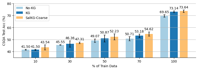
Figure 4: Low-Resource Learning. CSQA test accuracy for No-KG, KG, and SalKG-Coarse, when using varying amounts of training data.

A.12 Analyzing the Impact of Coarse Explanations

SalKG-Coarse is based on the insight that KG information may help the model on some instances but hurt on others. Thus, even if KG outperforms No-KG on average, No-KG may still correctly predict some instances that KG got wrong. SalKG-Coarse takes advantage of such complementary predictions between No-KG and KG, in order to achieve performance higher than $\max(\text{No-KG},\text{KG})$. As shown by RoBERTa+PathGen and RoBERTa+RN on OBQA (Table 6), SalKG-Coarse can still beat $\max(\text{No-KG},\text{KG},\text{No-KG}+\text{KG})$ even when No-KG outperforms KG.

In Table 14, we analyze the performance of BERT (i.e., No-KG), PathGen (i.e., KG), SalKG-Coarse (BERT+PathGen), and Oracle-Coarse (BERT+PathGen) on various sets of questions in CSQA. Due to computational constraints, each model’s performance here is reported for one seed (instead of using the protocol described in Sec. A.4), so these results are not directly comparable to those in Table 5. Through this performance breakdown, we can isolate the potential improvement contributed by each base model to SalKG-Coarse. We begin by looking at the questions for which SalKG-Coarse has no influence. These are the 46.01% of questions correctly answered by both models and the 33.92% of questions incorrectly answered by both models. Since SalKG-Coarse is trained to choose between the two models’ predictions, SalKG-Coarse’s output is fixed if both models make the same prediction. This leaves 20.07% of questions that were correctly answered by exactly one of the two models: 9.43% were from No-KG, while the other 10.64% were from KG. This 20.07% of constitutes the complementary predictions leveraged by SalKG-Coarse.

Based on this question-level analysis, we would estimate the Oracle-Coarse accuracy to be 66.08%, the percentage of questions that at least one model answered correctly. However, as stated in Sec. 3.1, coarse saliency targets are created at the answer choice level (not question level), which offers us more flexibility to choose between No-KG and KG. As a result, Oracle-Coarse’s accuracy is actually 68.57%. This leaves SalKG-Coarse (56.65%) significant room for improvement, perhaps through better model architecture and training.

Question Set	Question Percentage (%)
No-KG Correct	55.44
KG Correct	56.65
Only No-KG Correct	9.43
Only KG Correct	10.64
Both Correct	46.01
Both Incorrect	33.92
At Least One Incorrect	66.08
SalKG-Coarse Correct	56.65
Oracle-Coarse Correct	68.57

Table 14: Impact of Coarse Explanations. Using BERT+PathGen on CSQA, we present a performance breakdown for various question sets, in order to analyze why SalKG-Coarse is able to beat No-KG and KG.

A.13 Comparing Salient and Non-Salient KG Units

This paper explores learning from explanations of KG units’ saliency (i.e., usefulness). Overall, our focus is on how using salient KG units can yield improve model performance. In this subsection, we also analyze whether salient and non-salient KG units, as determined by our coarse/fine explanation methods, can differ in other ways that are not directly related to performance (Table 15). For both coarse and fine explanations, we use the BERT+MHGRN model on CSQA, where MHGRN is a node-based graph encoder (Sec. 4.2). Recall that Q nodes and A nodes are nodes (i.e., concepts) mentioned in the given question and answer choice, respectively (Sec. 6.1).

For coarse explanations, we use the ensemble-based explanations introduced in Sec. 3.1. We compare salient and non-salient KGs with respect to the number of nodes in the KG (# nodes), percentage of Q nodes in the KG (% Q nodes), percentage of A nodes in the KG (% A nodes), clustering coefficient (cluster coeff.), and average node degree (degree). These results are shown in Table 15a. We see that these metrics are not very discriminative, as salient and non-salient KGs perform similarly on all of these metrics.

For fine explanations, we use the Grad-based explanations described in Sec. 3.2 and Sec. A.3. We compare salient and non-salient nodes with respect to the percentage of Q nodes among salient/non-salient nodes in the KG (% Q nodes), percentage of A nodes among salient/non-salient nodes in the KG (% A nodes), and node degree (degree). These results are shown in Table 15b. Here, we see that %Q nodes and %A nodes are actually quite discriminative metrics between salient and non-salient nodes. On average, the percentage of Q nodes among salient nodes (16.84%) is 56.07% greater than the percentage of Q nodes among non-salient nodes (10.79%). Similarly, on average, the percentage of A nodes among salient nodes (10.00%) is 65.02% greater than the percentage of Q nodes among non-salient nodes (6.06%). However, compared to %Q nodes and %A nodes, degree is not as discriminative. This indicates that the difference between salient and non-salient nodes may be more semantic than structural.

Metric	Salient	Non-Salient
# nodes	125.88	120.57
% Q nodes	9.09	9.17
% A nodes	2.94	3.12
cluster coeff.	4.26E-1	4.25E-1
degree	9.89	9.78

(a) Salient vs. Non-Salient KGs.

Metric	Salient	Non-Salient
% Q nodes	16.84	10.79
% A nodes	10.00	6.06
degree	15.41	13.11

(b) Salient vs. Non-Salient Nodes.

Table 15: Salient vs. Non-Salient KG Units. Using BERT+MHGRN on CSQA, we compare salient and non-salient KG units. In (a), we compare salient and non-salient KGs, as determined by coarse explanations. In (b), we compare salient and non-salient nodes, as determined by fine explanations.

A.14 Robustness to KG Perturbation

Table 16 shows the CSQA performance of KG and SalKG models subjected to different forms of KG perturbation. Relation perturbation (Relation) permutes the relation labels of all edges in the KG, while node perturbation (Node) permutes the node labels of all nodes in the KG. These perturbation methods are designed to alter the semantics of the KG. For relation perturbation and node perturbation, SalKG-Coarse (Node) performs best on almost all settings, with KG (Node) barely beating SalKG-Coarse for node perturbation on BERT+PathGen. However, with KG perturbation, SalKG-Hybrid does not perform as well, sometimes even worse than KG and SalKG-Fine. This may be because SalKG-Hybrid relies most heavily on fine explanations, making it especially sensitive to KG perturbation.

We also compare these KG-perturbed models to models without any KG perturbation. As expected, across all settings, the KG-perturbed models outperform the non-KG-perturbed models. Interestingly, we find that SalKG-Coarse is most robust to KG perturbation. For BERT+RN and RoBERTa+RN, SalKG-Coarse (Relation) is less than 1% worse than SalKG-Coarse. This makes sense, since SalKG-Coarse relies least on the KG. For a given instance, SalKG-Coarse has the option to completely ignore KG information when making its prediction. When the KG is perturbed, it would be advantageous for SalKG-Coarse to focus only on the text input.

	CSQA Test Accuracy (%)
	MHGRN		PathGen		RN
Model	BERT	RoBERTa	BERT	RoBERTa	BERT	RoBERTa
KG (Relation)	52.89 ($\pm$0.73)	67.41 ($\pm$0.84)	52.35 ($\pm$0.60)	70.08 ($\pm$0.38)	54.15 ($\pm$0.40)	68.95 ($\pm$1.58)
SalKG-Coarse (Relation)	55.86 ($\pm$0.48)	72.53 ($\pm$0.50)	56.07 ($\pm$0.44)	71.55 ($\pm$0.85)	56.93 ($\pm$0.51)	72.43 ($\pm$0.96)
SalKG-Fine (Relation)	52.58 ($\pm$0.70)	68.84 ($\pm$0.67)	53.32 ($\pm$0.61)	71.23 ($\pm$1.21)	53.94 ($\pm$0.63)	69.80 ($\pm$0.64)
SalKG-Hybrid (Relation)	51.28 ($\pm$0.70)	69.84 ($\pm$0.57)	53.33 ($\pm$0.55)	70.34 ($\pm$1.03)	52.41 ($\pm$1.11)	68.77 ($\pm$0.80)
KG (Node)	53.63 ($\pm$0.70)	67.35 ($\pm$0.41)	55.60 ($\pm$0.16)	70.51 ($\pm$1.69)	54.15 ($\pm$2.27)	70.48 ($\pm$1.71)
SalKG-Coarse (Node)	55.75 ($\pm$0.60)	71.83 ($\pm$0.60)	55.43 ($\pm$0.55)	71.36 ($\pm$0.81)	56.14 ($\pm$0.73)	71.20 ($\pm$0.72)
SalKG-Fine (Node)	53.60 ($\pm$0.83)	66.81 ($\pm$1.09)	53.13 ($\pm$0.99)	70.80 ($\pm$1.55)	54.02 ($\pm$0.84)	71.08 ($\pm$1.02)
SalKG-Hybrid (Node)	51.14 ($\pm$1.03)	69.58 ($\pm$0.77)	50.80 ($\pm$0.83)	69.85 ($\pm$0.72)	53.24 ($\pm$0.72)	69.57 ($\pm$1.14)
KG	57.48 ($\pm$0.89)	73.14 ($\pm$0.78)	56.54 ($\pm$0.73)	72.58 ($\pm$0.57)	56.46 ($\pm$1.22)	71.37 ($\pm$1.20)
SalKG-Coarse	57.98 ($\pm$0.90)	73.64 ($\pm$1.05)	57.75 ($\pm$0.77)	73.07 ($\pm$0.25)	57.50 ($\pm$1.25)	73.11 ($\pm$1.13)
SalKG-Fine	54.36 ($\pm$2.34)	70.00 ($\pm$0.81)	54.39 ($\pm$2.03)	72.12 ($\pm$0.91)	54.30 ($\pm$1.41)	71.64 ($\pm$1.51)
SalKG-Hybrid	58.70 ($\pm$0.65)	73.37 ($\pm$0.12)	59.87 ($\pm$0.42)	72.67 ($\pm$0.65)	58.78 ($\pm$0.14)	74.13 ($\pm$0.71)

Table 16: SalKG Performance Comparison on CSQA with Perturbed KGs. Best performance in bold.

	CSQA p-values
	MHGRN		PathGen		RN
Model	BERT	RoBERTa	BERT	RoBERTa	BERT	RoBERTa
Best SalKG Model vs. Best Non-SalKG Model	0.1235	0.4238	0.0701	0.2690	0.1336	0.0441

Table 17: SalKG T-Test Results on CSQA. For each setting in Table 5, we perform the T-test between the best SalKG model and the best non-SalKG model.

	OBQA p-values			CODAH p-values
Model (RoBERTa)	MHGRN	PathGen	RN	MHGRN	PathGen
Best SalKG Model vs. Best Non-SalKG Model	0.2909	0.8890	0.0005	0.1223	0.2823

Table 18: SalKG T-Test Results on OBQA and CODAH. For each setting in Table 6, we perform the T-test between the best SalKG model and the best non-SalKG model.

A.15 Statistical Significance of Main Results

In this section, we verify the statistical significance of our results in Sec. 6.2. For each setting in Tables 5-6 (except RoBERTa+PathGen on CODAH), we perform the two-sided unpaired T-test with unequal variance between the best SalKG model and the best non-SalKG model. The $p$-values are shown in Tables 17-18.

If we use threshold $\alpha=0.1$ (i.e., $p<0.1$), then we find that SalKG yields statistically significant improvements on CSQA BERT+PathGen, CSQA RN+RoBERTa, and OBQA RN+RoBERTa. If we use threshold $\alpha=0.05$ (i.e., $p<0.05$), then we find that SalKG yields statistically significant improvements on CSQA RN+RoBERTa and OBQA RN+RoBERTa. In particular, the improvement on OBQA RN+RoBERTa is very statistically significant, with $p=0.0005$. Our T-test results show that SalKG can produce significant performance gains on a number of model-dataset settings, while yielding competitive performance in other settings.

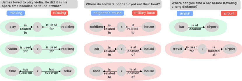
Figure 5: Examples of coarse/fine saliency explanations. Illustration of examples presented in Sec. 6.4. Blue denotes given answer choice, while red denotes target answer.

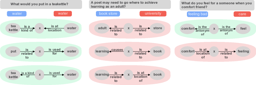
Figure 6: More examples of coarse/fine saliency explanations. Illustration of examples presented in Sec. A.16. Blue denotes given answer choice, while red denotes target answer.

A.16 Case Studies: Qualitative Analysis of KG Saliency Explanations

In this section, we build upon Sec. 6.4 and illustrate more examples of coarse/fine explanations created from BERT+PathGen on CSQA, with 1-hop or 2-hop paths as fine units. Notice that 2-hop paths consist of two nodes and two relations, with the intermediate node replaced with a placeholder node x, following [13]. By constructing 2-hop paths this way, the model is able to learn from more general 2-hop paths.

First, for coarse explanations, we provide more examples of positive (i.e., useful) and negative KGs.

• For the positive KG example, the question is What would you put in a teakettle?, the answer choice is water, and the target answer is water. Its paths are: (1) teakettle –[is a kind of]–> x <–[is at location]– water , (2) put –[is related to]–> x –[is used for]–> water , and (3) teakettle –[is a kind of]–> x –[is used for]–> water .

• For the negative KG example, the question is A poet may need to go where to achieve learning as an adult?, the answer choice is book store, and the target answer is university. Its paths are: (1) adult <–[is related to]– x –[is related to]–> store , (2) learning <–[causes]– x <–[is related to]– book , and (3) learning –[is related to]–> x –[is at location of]–> book .

Second, we provide more examples of fine explanations. Here, the question is What do you feel for a someone when you comfort friend?, the answer choice is feeling bad, and target answer is care. The positive path is: comfort <–[is the antonym of]– x –[is the antonym of]–> feel . The negative path is: comfort –[is at location of]–> x –[is related to]–> feeling .

The examples from Sec. 6.4 are shown in Fig. 5. The examples introduced in this subsection (Sec. A.16) are shown in Fig. 6. Again, in the coarse/fine explanations, we can roughly see that the positive KGs/paths tend to be useful for predicting the correct answer, and vice versa. However, note that the model’s judgment of KG/path usefulness may not necessarily align with human judgment [45].

A.17 User Studies: Quantitative Analysis of KG Saliency Explanations

To better understand the role and limitations of KG saliency explanations, we quantitatively analyze KG saliency explanations in the context of two user studies. In both user studies, the goal is to measure KG saliency explanations’ plausibility, i.e., how closely the explanations align with human judgment.

Note that explanation plausibility is orthogonal to our paper’s main claims, since we argue that KG saliency explanations can be used as additional supervision for improving performance, not that the explanations are plausible. Nonetheless, these user studies may still provide some useful insights about KG saliency explanations.

A.17.1 User Study 1: Coarse Saliency Explanations

The first user study measures how well the coarse (graph-level) explanations align with human judgment of usefulness. Given a RoBERTa+PathGen model, we begin by uniformly sampling 25 high-saliency (positive) KGs and 25 low-saliency (negative) KGs from the CSQA training set. Recall that whether a KG is high-saliency or low-saliency was determined by coarse explanations (Sec. 3.1) generated with respect to the given model.

Graph Type	Usefulness Score
High-Saliency Graph	0.929 ± 0.734
Low-Saliency Graph	0.935 ± 0.764

Table 19: Human Evaluation of Coarse Saliency Explanations. Human-annotated usefulness scores for high- (positive) and low- (negative) saliency graphs.

Note that each KG corresponds to one answer choice of a question, so each question in CSQA has up to five corresponding KGs. To ensure that none of the KGs in our sample come from the same question, we ended up pruning two high-saliency and two low-saliency KGs, yielding a final sample of 23 high-saliency and 23 low-saliency KGs.

Since a KG can contain hundreds of paths, it is not feasible to ask humans to evaluate the entire KG’s usefulness. Thus, as a very rough representation of the KG, we uniformly sampled three paths from the KG. Then, for each KG, we asked ten human annotators to score each of the three paths’ usefulness for predicting the same answer choice predicted by the RoBERTa+PathGen model. To score the paths, all annotators were also given the question, correct answer, and model’s predicted answer. The paths were scored on the following 0-2 scale:

• 0 = definitely not useful (i.e., this path is either irrelevant or would cause someone to NOT select the model’s predicted answer)

• 1 = possibly useful (i.e., this path provides some support for selecting the model’s predicted answer)

• 2 = definitely useful (i.e., this path provides strong support for selecting the model’s predicted answer)

Finally, each KG’s score is computed as the mean of its three constituent path scores. Below, we show the mean and standard deviation scores for high-saliency and low-saliency graphs. We find that the two graph types have similar mean usefulness scores, while also having relatively large standard deviations. This suggests that coarse saliency explanations do not align strongly with human judgment. One key limitation of this study is that the three sampled paths may not be representative of the entire KG. In the future, we plan to redesign the user study to provide annotators a more comprehensive representation of the KG to evaluate.

A.17.2 User Study 2: Fine Saliency Explanations

The second user study measures how well the fine (path-level) explanations align with human judgment of usefulness. Given a RoBERTa+PathGen model trained on CSQA, we begin by uniformly sampling 25 correctly answered questions and 25 incorrectly answered questions from the CSQA training set. For each question, we take the model’s predicted answer choice and the KG corresponding to the predicted answer choice, then select: (1) the path with the highest fine saliency score, (2) the path with median fine saliency score, and (3) the path with the lowest saliency score. To get finer-grained saliency signal in this study, we consider the raw fine saliency scores, instead of the binarized fine explanations actually used to regularize the model. Recall that a path’s fine saliency score (Sec. 3.2) is calculated with respect to the given model.

Next, we asked ten human annotators to score each path’s usefulness for predicting the same answer choice predicted by the RoBERTa+PathGen model. Like before, to score the paths, all annotators were also given the question, correct answer, and model’s predicted answer. Again, the paths were scored on the following 0-2 scale:

• 0 = definitely not useful (i.e., this path is either irrelevant or would cause someone to NOT select the model’s predicted answer)

• 1 = possibly useful (i.e., this path provides some support for selecting the model’s predicted answer)

• 2 = definitely useful (i.e., this path provides strong support for selecting the model’s predicted answer)

Below, we show the mean scores for high-saliency, median-saliency, and low-saliency paths. We display these scores for paths from all predictions, correct predictions, and incorrect predictions. Overall, we find that the three path types have similar mean usefulness scores, although the mean score for median-saliency paths is somewhat higher than the other two path types’. Still, the standard deviations for all scores are relatively large, so this trend may not be meaningful. These results suggest that fine saliency explanations do not strongly align with human judgment. Additionally, we find that the path usefulness scores for correct predictions tend to be higher than those from incorrect predictions. This makes sense, since, intuitively, a model is more likely to predict the correct answer if it is using more useful knowledge as context.

Path Type	Usefulness Score (All Preds)	Usefulness Score (Correct Preds)	Usefulness Score (Incorrect Preds)
High-Saliency Path	1.091 ± 0.805	1.298 ± 0.782	0.884 ± 0.776
Med-Saliency Path	1.222 ± 0.769	1.320 ± 0.729	1.124 ± 0.798
Low-Saliency Path	1.060 ± 0.733	1.182 ± 0.730	0.938 ± 0.717

Table 20: Human Evaluation of Fine Saliency Explanations. Human-annotated usefulness scores for high-, median-, and low-saliency paths. We display the usefulness scores for paths from all predictions, correct predictions, and incorrect predictions.

User Study	Fleiss’ Kappa
Coarse Explanations	0.2089
Fine Explanations	0.1296

Table 21: Inter-Annotator Agreement for Explanation User Studies. Using Fleiss’ kappa, we measure the inter-annotator agreement for the human evaluation of coarse and fine saliency explanations. In both settings, the inter-annotator agreement is relatively low.

A.17.3 Inter-Annotator Agreement

Here, we measure inter-annotator agreement for both user studies, using Fleiss’ kappa. For the user study of coarse explanations, the kappa score is 0.2089, which is on the borderline of slight agreement and fair agreement. For the user study of fine explanations, the kappa score is 0.1296, which indicates slight agreement.

These low kappa scores show that even humans can hardly agree on whether the coarse/fine explanations are useful. Therefore, it may not always be beneficial to measure explanation quality in terms of alignment with human judgment. Moreover, this shows that weak alignment with human judgment does not necessarily imply poor explanation quality.

A.17.4 Analysis

In our user studies, we did not find strong evidence that coarse/fine saliency explanations align well with human judgment. However, we also found that human annotators had very low agreement about the usefulness of the explanations, which suggests that alignment with human judgment may not be the best measure of explanation quality.

In light of this, we emphasize that the user study results do not contradict our paper’s conclusions, as our work does not claim that the generated saliency explanations are plausible. Rather, we merely claim that using KG-based saliency explanations as additional supervision to regularize KG-augmented models can yield higher performance.

Our work appeals to the view that an explanation’s quality should be measured by how well it distills knowledge for improving performance on some task [43]. Furthermore, the results of our user studies are actually in line with the conclusions from [45], which found that KG-augmented models can effectively leverage KG information to improve performance, but in a manner that may not make sense to humans.

A.18 Training Hyperparameters

Since we consider a very large number of models and settings in our experiments, we only describe the core hyperparameters here. Let bsz denote batch size, let $\text{lr}_{\text{text}}$ denote text encoder learning rate, let $\text{lr}_{\text{graph}}$ denote graph encoder learning rate, and let $\text{lr}_{\text{task}}$ denote task predictor learning rate. Across all models (both baselines and SalKG), we generally used the following hyperparameter sweeps: $\text{bsz}=[8,16,32,64]$, $\text{lr}_{\text{text}}=[1\mathrm{e}{-5},2\mathrm{e}{-5},3\mathrm{e}{-5},5\mathrm{e}{-5}]$, $\text{lr}_{\text{graph}}=[1\mathrm{e}{-4},2\mathrm{e}{-4},3\mathrm{e}{-4},5\mathrm{e}{-4}]$, and $\text{lr}_{\text{task}}=[1\mathrm{e}{-4},2\mathrm{e}{-4},3\mathrm{e}{-4},5\mathrm{e}{-4}]$. For CSQA and OBQA, we set the maximum number of epochs to 100. For CODAH, we set the maximum number of epochs to 30. For all three datasets, we used early stopping with a patience of 5 epochs. For more details about hyperparameters, please refer to our code repository.

A.19 Computational Costs and Resources

Since the SalKG pipeline (as well as Oracle, Random, and Heuristic) involves training models across multiple stages, its computational costs are considerably greater than those from just training a No-KG or KG model individually. Specifically, the pipeline involves: (1) training the No-KG and KG models; (2) creating coarse/fine explanations from the No-KG and KG models; (3) training the SalKG-Coarse model; (4) training the SalKG-Fine model; and (5) training the SalKG-Hybrid model. In particular, using the Occl method to create fine explanations can be especially costly since it requires $n+1$ KG model forward passes per KG, where $n$ is the number of units in the given KG. Also, if we tune the $T$ or $k$ thresholds comprehensively, then the total training time further increases. For reference, each of our experiments was run on one NVIDIA Quadro RTX 8000 GPU.

Nonetheless, since we are the first to propose regularizing KG-augmented models with saliency explanations, it is expected that not all components of our method will already be fully optimized. That is, the goal of our work is simply to introduce a new paradigm for training KG-augmented models and demonstrate its potential by showing that it can yield improved performance. Certainly, there are various parts of the SalKG pipeline whose efficiency can be improved. For example, we could explore faster explanation generation via some KG-specific heuristic/approximation, training SalKG-Hybrid with coarse/fine explanations in a single step (instead of Steps 3-5 above), or generating explanations that can cover multiple instances at a time. Such potential improvements could be interesting directions for future work.

A.20 Related Work (Extended)

Text-Based Explanations

Many works have been proposed for explaining the predictions of language models, especially PLMs. Although some of these works focus on abstractive (free-text) explanations [44, 50, 64], most aim to provide extractive explanations which highlight salient tokens in the model’s text input. Such extractive explanations typically use either gradient-based [51, 29, 10], attention-based [40, 53, 14, 25], and occlusion-based [12, 42, 22, 30] feature attribution methods. How feature attribution methods should be chosen remains an open question and the subject of much recent debate [2, 59, 48, 20]. While SalKG also uses feature attribution methods (e.g., G$\times$I) to create extractive explanations, our study is limited to explanations regarding KG-augmented models’ graph inputs.

Graph-Based Explanations

There are also methods proposing extractive explanations for graph encoders, especially GNNs. Such explanations are designed to point out components in the graph input that contribute most to the model’s prediction. Some GNNs use attention for pooling, which naturally highlights nodes with higher attention weights [27, 26]. More sophisticated approaches use post-hoc optimization to identify salient nodes [19, 62] or subgraphs [62].

Unlike individual PLMs and graph encoders, KG-augmented models take both text and graph inputs. The KG-augmented model’s graph encoder usually computes graph embeddings via attention pooling of nodes/paths, and the attention weights can be used to explain which nodes/paths in the input KG are salient [31, 13, 34, 56, 60]. These KG explanations can be interpreted as identifying knowledge in the KG that is complementary to the knowledge encoded in the PLM. However, there is little work on how such KG explanations should be used. SalKG considers graph-based extractive explanations of KG-augmented models, but focuses more on how explanations are used rather than created.

Learning From Model Explanations

To improve the model’s learning, explanations can be used in a diverse range of ways, including as extra supervision or regularization [43, 17, 41, 1], pruned inputs [21, 3, 28], additional inputs [16, 8], and intermediate variables [58, 66, 44]. The most similar work to ours is [43], which proposed training a student model to mimic a teacher model’s predictions by regularizing the student model’s attention via text explanations created from the teacher model. However, [43] aims to evaluate explanations, while our goal is to improve performance via explanations. Still, methods for learning from explanations have largely focused on domains like text and images, as opposed to graphs. To the best of our knowledge, SalKG is the first work to train KG-augmented models using KG explanations as supervision.

A.21 Societal Impact

Our proposed SalKG approach for learning from KG explanations can be applied to any KG-augmented model and can be adapted from any off-the-shelf saliency method. This enables KG-augmented models to improve generalization ability and learn more efficiently from data, thus yielding better performance while requiring less labeled data. However, in the present version of SalKG, this generalization ability and data efficiency comes with increased computational costs, as described in Sec. A.19. In the future, we plan to explore methods for improving generalization and data efficiency while minimizing computational costs.

References

- [1] Jacob Andreas, Dan Klein, and Sergey Levine. Learning with latent language. arXiv preprint arXiv:1711.00482, 2017.
- [2] Jasmijn Bastings and Katja Filippova. The elephant in the interpretability room: Why use attention as explanation when we have saliency methods? arXiv preprint arXiv:2010.05607, 2020.
- [3] Joost Bastings, Wilker Aziz, and Ivan Titov. Interpretable neural predictions with differentiable binary variables. arXiv preprint arXiv:1905.08160, 2019.
- [4] Peter W Battaglia, Jessica B Hamrick, Victor Bapst, Alvaro Sanchez-Gonzalez, Vinicius Zambaldi, Mateusz Malinowski, Andrea Tacchetti, David Raposo, Adam Santoro, Ryan Faulkner, et al. Relational inductive biases, deep learning, and graph networks. arXiv preprint arXiv:1806.01261, 2018.
- [5] Antoine Bosselut and Yejin Choi. Dynamic knowledge graph construction for zero-shot commonsense question answering. arXiv preprint arXiv:1911.03876, 2019.
- [6] Michael Chen, Mike D’Arcy, Alisa Liu, Jared Fernandez, and Doug Downey. CODAH: An adversarially-authored question answering dataset for common sense. In Proceedings of the 3rd Workshop on Evaluating Vector Space Representations for NLP, pages 63–69, Minneapolis, USA, June 2019. Association for Computational Linguistics.
- [7] Qian Chen, Xiaodan Zhu, Zhen-Hua Ling, Diana Inkpen, and Si Wei. Neural natural language inference models enhanced with external knowledge. arXiv preprint arXiv:1711.04289, 2017.
- [8] John D Co-Reyes, Abhishek Gupta, Suvansh Sanjeev, Nick Altieri, Jacob Andreas, John DeNero, Pieter Abbeel, and Sergey Levine. Guiding policies with language via meta-learning. arXiv preprint arXiv:1811.07882, 2018.
- [9] Ernest Davis and Gary Marcus. Commonsense reasoning and commonsense knowledge in artificial intelligence. Communications of the ACM, 58(9):92–103, 2015.
- [10] Misha Denil, Alban Demiraj, and Nando De Freitas. Extraction of salient sentences from labelled documents. arXiv preprint arXiv:1412.6815, 2014.
- [11] Jacob Devlin, Ming-Wei Chang, Kenton Lee, and Kristina Toutanova. BERT: Pre-training of deep bidirectional transformers for language understanding. In Proceedings of NAACL), pages 4171–4186, Minneapolis, Minnesota, June 2019. Association for Computational Linguistics.
- [12] Jay DeYoung, Sarthak Jain, Nazneen Fatema Rajani, Eric Lehman, Caiming Xiong, Richard Socher, and Byron C Wallace. Eraser: A benchmark to evaluate rationalized nlp models. arXiv preprint arXiv:1911.03429, 2019.
- [13] Yanlin Feng, Xinyue Chen, Bill Yuchen Lin, Peifeng Wang, Jun Yan, and Xiang Ren. Scalable multi-hop relational reasoning for knowledge-aware question answering. arXiv preprint arXiv:2005.00646, 2020.
- [14] Reza Ghaeini, Xiaoli Z Fern, and Prasad Tadepalli. Interpreting recurrent and attention-based neural models: a case study on natural language inference. arXiv preprint arXiv:1808.03894, 2018.
- [15] David Gunning. Machine common sense concept paper. arXiv preprint arXiv:1810.07528, 2018.
- [16] Peter Hase and Mohit Bansal. When can models learn from explanations? a formal framework for understanding the roles of explanation data. arXiv preprint arXiv:2102.02201, 2021.
- [17] Peter Hase, Shiyue Zhang, Harry Xie, and Mohit Bansal. Leakage-adjusted simulatability: Can models generate non-trivial explanations of their behavior in natural language? arXiv preprint arXiv:2010.04119, 2020.
- [18] Matthew Honnibal and Mark Johnson. An improved non-monotonic transition system for dependency parsing. In Proceedings of the 2015 Conference on Empirical Methods in Natural Language Processing, pages 1373–1378, Lisbon, Portugal, September 2015. Association for Computational Linguistics.
- [19] Qiang Huang, Makoto Yamada, Yuan Tian, Dinesh Singh, Dawei Yin, and Yi Chang. Graphlime: Local interpretable model explanations for graph neural networks. arXiv preprint arXiv:2001.06216, 2020.
- [20] Sarthak Jain and Byron C Wallace. Attention is not explanation. arXiv preprint arXiv:1902.10186, 2019.
- [21] Sarthak Jain, Sarah Wiegreffe, Yuval Pinter, and Byron C Wallace. Learning to faithfully rationalize by construction. arXiv preprint arXiv:2005.00115, 2020.
- [22] Akos Kádár, Grzegorz Chrupała, and Afra Alishahi. Representation of linguistic form and function in recurrent neural networks. Computational Linguistics, 43(4):761–780, 2017.
- [23] Tushar Khot, Peter Clark, Michal Guerquin, Peter Jansen, and Ashish Sabharwal. QASC: A dataset for question answering via sentence composition. In The Thirty-Fourth AAAI Conference on Artificial Intelligence, AAAI 2020, The Thirty-Second Innovative Applications of Artificial Intelligence Conference, IAAI 2020, The Tenth AAAI Symposium on Educational Advances in Artificial Intelligence, EAAI 2020, New York, NY, USA, February 7-12, 2020, pages 8082–8090. AAAI Press, 2020.
- [24] Zhenzhong Lan, Mingda Chen, Sebastian Goodman, Kevin Gimpel, Piyush Sharma, and Radu Soricut. Albert: A lite bert for self-supervised learning of language representations. arXiv preprint arXiv:1909.11942, 2019.
- [25] Jaesong Lee, Joong-Hwi Shin, and Jun-Seok Kim. Interactive visualization and manipulation of attention-based neural machine translation. In Proceedings of the 2017 Conference on Empirical Methods in Natural Language Processing: System Demonstrations, pages 121–126, 2017.
- [26] John Boaz Lee, Ryan Rossi, and Xiangnan Kong. Graph classification using structural attention. In Proceedings of the 24th ACM SIGKDD International Conference on Knowledge Discovery & Data Mining, pages 1666–1674, 2018.
- [27] Junhyun Lee, Inyeop Lee, and Jaewoo Kang. Self-attention graph pooling. In International Conference on Machine Learning, pages 3734–3743. PMLR, 2019.
- [28] Tao Lei, Regina Barzilay, and Tommi Jaakkola. Rationalizing neural predictions. arXiv preprint arXiv:1606.04155, 2016.
- [29] Jiwei Li, Xinlei Chen, Eduard Hovy, and Dan Jurafsky. Visualizing and understanding neural models in nlp. arXiv preprint arXiv:1506.01066, 2015.
- [30] Jiwei Li, Will Monroe, and Dan Jurafsky. Understanding neural networks through representation erasure. arXiv preprint arXiv:1612.08220, 2016.
- [31] Bill Yuchen Lin, Xinyue Chen, Jamin Chen, and Xiang Ren. KagNet: Knowledge-aware graph networks for commonsense reasoning. In Proceedings of EMNLP-IJCNLP, pages 2829–2839, Hong Kong, China, November 2019. Association for Computational Linguistics.
- [32] Bill Yuchen Lin, Wangchunshu Zhou, Ming Shen, Pei Zhou, Chandra Bhagavatula, Yejin Choi, and Xiang Ren. CommonGen: A constrained text generation challenge for generative commonsense reasoning. In Findings of the Association for Computational Linguistics: EMNLP 2020, pages 1823–1840, Online, November 2020. Association for Computational Linguistics.
- [33] Ye Liu, Yao Wan, Lifang He, Hao Peng, and Philip S Yu. Kg-bart: Knowledge graph-augmented bart for generative commonsense reasoning. arXiv preprint arXiv:2009.12677, 2020.
- [34] Ye Liu, Tao Yang, Zeyu You, Wei Fan, and Philip S Yu. Commonsense evidence generation and injection in reading comprehension. arXiv preprint arXiv:2005.05240, 2020.
- [35] Yinhan Liu, Myle Ott, Naman Goyal, Jingfei Du, Mandar Joshi, Danqi Chen, Omer Levy, Mike Lewis, Luke Zettlemoyer, and Veselin Stoyanov. Roberta: A robustly optimized bert pretraining approach. arXiv preprint arXiv:1907.11692, 2019.
- [36] Shangwen Lv, Daya Guo, Jingjing Xu, Duyu Tang, Nan Duan, Ming Gong, Linjun Shou, Daxin Jiang, Guihong Cao, and Songlin Hu. Graph-based reasoning over heterogeneous external knowledge for commonsense question answering. In Proceedings of the AAAI Conference on Artificial Intelligence, volume 34, pages 8449–8456, 2020.
- [37] Kaixin Ma, Jonathan Francis, Quanyang Lu, Eric Nyberg, and Alessandro Oltramari. Towards generalizable neuro-symbolic systems for commonsense question answering. In Proceedings of the First Workshop on Commonsense Inference in Natural Language Processing, pages 22–32, Hong Kong, China, November 2019. Association for Computational Linguistics.
- [38] Gary Marcus. Deep learning: A critical appraisal. arXiv preprint arXiv:1801.00631, 2018.
- [39] Todor Mihaylov, Peter Clark, Tushar Khot, and Ashish Sabharwal. Can a suit of armor conduct electricity? a new dataset for open book question answering. In Proceedings of the 2018 Conference on Empirical Methods in Natural Language Processing, pages 2381–2391, Brussels, Belgium, October-November 2018. Association for Computational Linguistics.
- [40] Akash Kumar Mohankumar, Preksha Nema, Sharan Narasimhan, Mitesh M Khapra, Balaji Vasan Srinivasan, and Balaraman Ravindran. Towards transparent and explainable attention models. arXiv preprint arXiv:2004.14243, 2020.
- [41] Sharan Narang, Colin Raffel, Katherine Lee, Adam Roberts, Noah Fiedel, and Karishma Malkan. Wt5?! training text-to-text models to explain their predictions. arXiv preprint arXiv:2004.14546, 2020.
- [42] Nina Poerner, Benjamin Roth, and Hinrich Schütze. Evaluating neural network explanation methods using hybrid documents and morphological agreement. arXiv preprint arXiv:1801.06422, 2018.
- [43] Danish Pruthi, Bhuwan Dhingra, Livio Baldini Soares, Michael Collins, Zachary C Lipton, Graham Neubig, and William W Cohen. Evaluating explanations: How much do explanations from the teacher aid students? arXiv preprint arXiv:2012.00893, 2020.
- [44] Nazneen Fatema Rajani, Bryan McCann, Caiming Xiong, and Richard Socher. Explain yourself! leveraging language models for commonsense reasoning. arXiv preprint arXiv:1906.02361, 2019.
- [45] Mrigank Raman, Aaron Chan, Siddhant Agarwal, Peifeng Wang, Hansen Wang, Sungchul Kim, Ryan Rossi, Handong Zhao, Nedim Lipka, and Xiang Ren. Learning to deceive knowledge graph augmented models via targeted perturbation. arXiv preprint arXiv:2010.12872, 2020.
- [46] Adam Santoro, David Raposo, David G Barrett, Mateusz Malinowski, Razvan Pascanu, Peter Battaglia, and Timothy Lillicrap. A simple neural network module for relational reasoning. In Advances in neural information processing systems, pages 4967–4976, 2017.
- [47] Michael Schlichtkrull, Thomas N Kipf, Peter Bloem, Rianne Van Den Berg, Ivan Titov, and Max Welling. Modeling relational data with graph convolutional networks. In European Semantic Web Conference, pages 593–607. Springer, 2018.
- [48] Sofia Serrano and Noah A Smith. Is attention interpretable? arXiv preprint arXiv:1906.03731, 2019.
- [49] Robyn Speer, Joshua Chin, and Catherine Havasi. Conceptnet 5.5: an open multilingual graph of general knowledge. In Proceedings of AAAI, pages 4444–4451, 2017.
- [50] Julia Strout, Ye Zhang, and Raymond J Mooney. Do human rationales improve machine explanations? arXiv preprint arXiv:1905.13714, 2019.
- [51] Mukund Sundararajan, Ankur Taly, and Qiqi Yan. Axiomatic attribution for deep networks. In International Conference on Machine Learning, pages 3319–3328. PMLR, 2017.
- [52] Alon Talmor, Jonathan Herzig, Nicholas Lourie, and Jonathan Berant. CommonsenseQA: A question answering challenge targeting commonsense knowledge. In Proceedings of the 2019 Conference of the North American Chapter of the Association for Computational Linguistics: Human Language Technologies, Volume 1 (Long and Short Papers), pages 4149–4158, Minneapolis, Minnesota, June 2019. Association for Computational Linguistics.
- [53] Martin Tutek and Jan Šnajder. Staying true to your word:(how) can attention become explanation? arXiv preprint arXiv:2005.09379, 2020.
- [54] Ashish Vaswani, Noam Shazeer, Niki Parmar, Jakob Uszkoreit, Llion Jones, Aidan N Gomez, Lukasz Kaiser, and Illia Polosukhin. Attention is all you need. arXiv preprint arXiv:1706.03762, 2017.
- [55] Petar Veličković, Guillem Cucurull, Arantxa Casanova, Adriana Romero, Pietro Lio, and Yoshua Bengio. Graph attention networks. arXiv preprint arXiv:1710.10903, 2017.
- [56] Peifeng Wang, Nanyun Peng, Pedro Szekely, and Xiang Ren. Connecting the dots: A knowledgeable path generator for commonsense question answering. arXiv preprint arXiv:2005.00691, 2020.
- [57] Xiaoyan Wang, Pavan Kapanipathi, Ryan Musa, Mo Yu, Kartik Talamadupula, Ibrahim Abdelaziz, Maria Chang, Achille Fokoue, Bassem Makni, Nicholas Mattei, et al. Improving natural language inference using external knowledge in the science questions domain. In Proceedings of the AAAI Conference on Artificial Intelligence, volume 33, pages 7208–7215, 2019.
- [58] Sarah Wiegreffe, Ana Marasovic, and Noah A Smith. Measuring association between labels and free-text rationales. arXiv preprint arXiv:2010.12762, 2020.
- [59] Sarah Wiegreffe and Yuval Pinter. Attention is not not explanation. arXiv preprint arXiv:1908.04626, 2019.
- [60] Jun Yan, Mrigank Raman, Aaron Chan, Tianyu Zhang, Ryan Rossi, Handong Zhao, Sungchul Kim, Nedim Lipka, and Xiang Ren. Learning contextualized knowledge structures for commonsense reasoning. arXiv preprint arXiv:2010.12873, 2020.
- [61] Michihiro Yasunaga, Hongyu Ren, Antoine Bosselut, Percy Liang, and Jure Leskovec. Qa-gnn: Reasoning with language models and knowledge graphs for question answering. arXiv preprint arXiv:2104.06378, 2021.
- [62] Zhitao Ying, Dylan Bourgeois, Jiaxuan You, Marinka Zitnik, and Jure Leskovec. Gnnexplainer: Generating explanations for graph neural networks. In Advances in neural information processing systems, pages 9244–9255, 2019.
- [63] Rowan Zellers, Yonatan Bisk, Roy Schwartz, and Yejin Choi. Swag: A large-scale adversarial dataset for grounded commonsense inference. arXiv preprint arXiv:1808.05326, 2018.
- [64] Xinyan Zhao and VG Vydiswaran. Lirex: Augmenting language inference with relevant explanation. arXiv preprint arXiv:2012.09157, 2020.
- [65] Hao Zhou, Tom Young, Minlie Huang, Haizhou Zhao, Jingfang Xu, and Xiaoyan Zhu. Commonsense knowledge aware conversation generation with graph attention. In IJCAI, pages 4623–4629, 2018.
- [66] Wangchunshu Zhou, Jinyi Hu, Hanlin Zhang, Xiaodan Liang, Maosong Sun, Chenyan Xiong, and Jian Tang. Towards interpretable natural language understanding with explanations as latent variables. arXiv preprint arXiv:2011.05268, 2020.