Catalog of One-side Head–Tail Galaxies in the FIRST Survey

Abstract

One-side head–tail (OHT) galaxies are radio galaxies with a peculiar shape. They usually appear in galaxy clusters, but they have never been cataloged systematically. We design an automatic procedure to search for them in the Faint Images of the Radio Sky at Twenty-Centimeters source catalog and compile a sample with 115 HT candidates. After cross-checking with the Sloan Digital Sky Survey photometric data and catalogs of galaxy clusters, we find that 69 of them are possible OHT galaxies. Most of them are close to the center of galaxy clusters. The lengths of their tails do not correlate with the projection distance to the center of the nearest galaxy clusters, but show weak anticorrelation with the cluster richness, and are inversely proportional to the radial velocity differences between clusters and host galaxies. Our catalog provides a unique sample to study this special type of radio galaxies.

1 Introduction

Radio galaxies are galaxies with high radio luminosity and relativistic particle emission. They have been studied for decades of years and show various morphologies(Miley, 1980; Proctor, 2011; Srivastava & Singal, 2020), which are closely related to the activities of their central active galactic nucleus (AGN), environment, and local galaxy richness(Feretti & Giovannini, 2008; Miraghaei & Best, 2017). The morphological classification of radio galaxies could provide useful information on the mechanism involved and act as a tracer of the intragalatic environment.

Proctor (2011) systematically examined the Faint Images of the Radio Sky at Twenty-Centimeters (FIRST; Becker et al., 1995) catalog and assorted sources by the number of member components. They presented 15 types of radio sources, including wide-angle tail (WAT), narrow-angle tail (NAT), core–jet, W-shaped, X-shaped, and so on.

The Radio Galaxy Zoo project (Banfield et al., 2015) provides a different approach. It recruited thousands of volunteers to do a visual inspection of the host galaxy and radio morphology with the FIRST and optical images (Garon et al., 2019).

There is a special type of radio galaxy—the head–tail (HT) —which has not been systematically searched for. The first HT was discovered in the Perseus cluster (Ryle & Windram, 1968). Miley et al. (1972) nominated these remarkable radio galaxies as HT galaxies and interpreted them as radio trails along trajectories through a dense intergalactic medium. Because WATs and NATs have similar bright heads and long faint tails, they are also sometimes mentioned as HT galaxies (e.g. Mao et al., 2009; Pratley et al., 2013).

This paper will focus on the one-sided head–tail (hereafter OHT) galaxies. Unlike WATs or NATs, they have only one unresolved tail. Some of them have been resolved as NATs with high-resolution observations (Terni de Gregory et al., 2017). so they are also called narrow HT (Terni de Gregory et al., 2017), and sometimes head-tailed galaxies for simplicity (e.g. Jones & McAdam, 1996; Yu et al., 2018; Srivastava & Singal, 2020). In this paper, we use the term HT to represent all three types: NAT, WAT, and OHT.

It is still unclear how the tails of OHTs formed. A possible explanation for the formation of such a structure may be the existence of a massive structure such as a galaxy cluster that makes the HT galaxy infall with a high velocity, resulting in the merger of two radiation lobes along the opposite direction of motion(O’Neill et al., 2019).

However, most known OHTs are by-products of cluster studies. This fact may bias our understanding of them. To explore their situation in a more general way, we need a fair sample. The FIRST project based on the Very Large Array (VLA) is a useful radio source catalog. It is a project designed to produce the radio equivalent of the Palomar Observatory Sky Survey over 10,000 square degrees of the north and south Galactic caps. Compared with other available radio sky surveys such as the NRAO/VLA Sky Survey(Condon et al., 1998) and the TIFR GMRT Sky Survey(Intema et al., 2017), FIRST has a much higher resolution, which is crucial to our study. The ongoing LOFAR Two-meter Sky Survey (LoTSS; Shimwell et al., 2017, 2019) will provide more helpful data in the near future.

This paper is organized as follows. In Section 2, we describe the preliminary selection criteria of HT-like structures in FIRST. Their optical identification is presented in Section 3. Section 4 concerns cluster checking. Properties of this sample are presented in Section 5. Section 6 contains our summary and conclusions.

2 radio identification

The FIRST Survey used the VLA in its B configuration centered at 1.4 GHz from 1993 through 2011 and acquired 3 minutes snapshots covering about 10,575 square degrees of sky(Becker et al., 1995). Its latest source catalog, which was released on 2014 December 17, contains 946,432 sources. They are derived from fitting the flux density of each source with an elliptical Gaussian(White et al., 1997). The peak, integrated flux densities, and sizes in the catalog provide a good representation of the source morphology.

Considering the particular shape of OHT sources, we design a straightforward routine to identify them from the radio catalog. We start with elongated sources which look like a “tail”, and search for bright sources, which could be a “head”, on the tip of them. If their relative positions, alignments, and brightness satisfy the given criteria, we combine them as HT structures.

2.1 “Tail”

The lowest signal-to-noise ratio (S/N) of FIRST sources is 5. To get rid of ambiguous radio sources in the catalog, we focus on sources with a S/N larger than 10. Since the angular resolution of FIRST is 5^′′, we only care about resolved sources and constrain the half major and minor axes (fMaj and fMin) derived from the elliptical Gaussian model larger than 5^′′. There are 453,346 sources satisfying these two basic conditions in the catalog.

The tail of an OHT source is always elongated, while the beam shape of the FIRST survey is round. So the ratio between the major and minor axes (ellipticity, e = fMaj/fMin) is the main difference between point sources and extended sources in the FIRST catalog. The ellipticity histogram of all 453,346 sources is given in Fig.1. Considering tails could be short due to the projection effect, we adopt a conservative ellipticity value e $>$ 1.5 as our tail selection criterion to include more possible candidates. With this criterion, 49,086 “tail” sources are sifted out.

Figure 1: The ellipticity distribution of 453,346 FIRST sources. The red line refers to the ellipticity e = 1.5.

2.2 “Head”

All known OHT sources show bright radio cores close to the host galaxy, if not overlapping with it. The core is called the “head”. So we go through all tail candidates to check if there is any bright source around them. On one hand, the head’s peak flux should be brighter than the value of the tail: fPeak_h $>$ fPeak_t. On the other hand, the ellipticity of the head should be smaller than the tail: $e_{h}$ $<$ $e_{t}$. Considering that some heads may not have close contact with the tail, we set a slightly large searching radius r_t = 1.5 fMaj_t, as Fig. 2 illustrates.The brightest source within this radius is chosen as the “head” associated with the “tail”. There are 9704 tails with a head beside a tail.

To remove bright sources overlapping with tails by chance, we add an additional condition – the phase-angle offset $\alpha$ between the tail and the head (shown in Fig.2) should be less than 20^∘ to guarantee their alignment, because both of them follow the trajectories of the host galaxy.

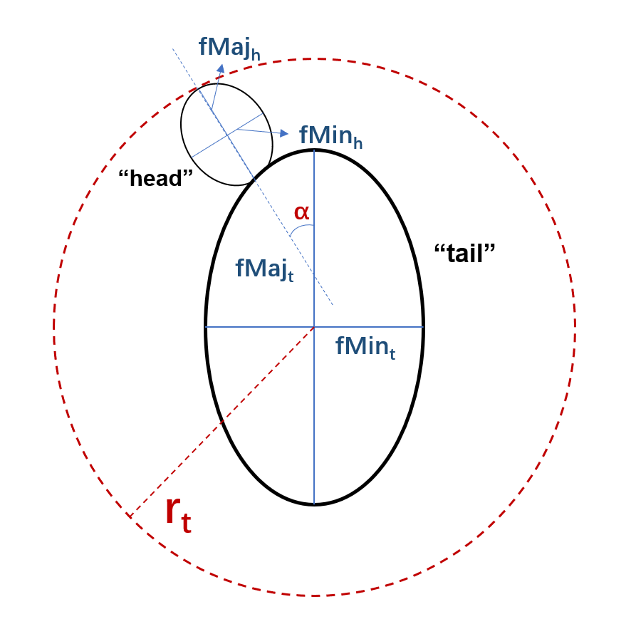
Figure 2: The red dashed circle r_t refers to the range of 1.5 times the half major axes of the tail (fMaj_t); within this range, we identify the brightest source as the “head”. $\alpha$ in red is the angle between the long axis of the tail and the head, which is the phase-angle offset used to determine whether the “head” and “tail” are aligned.

The histogram distribution of $\alpha$ is given by Fig.3. It is clear that $\alpha<20^{\circ}$ is not strict. A flow chart (Fig.4) is given to show our selection process more intuitively. After the head searching, we get 5564 head–tail combinations as our HT structures.

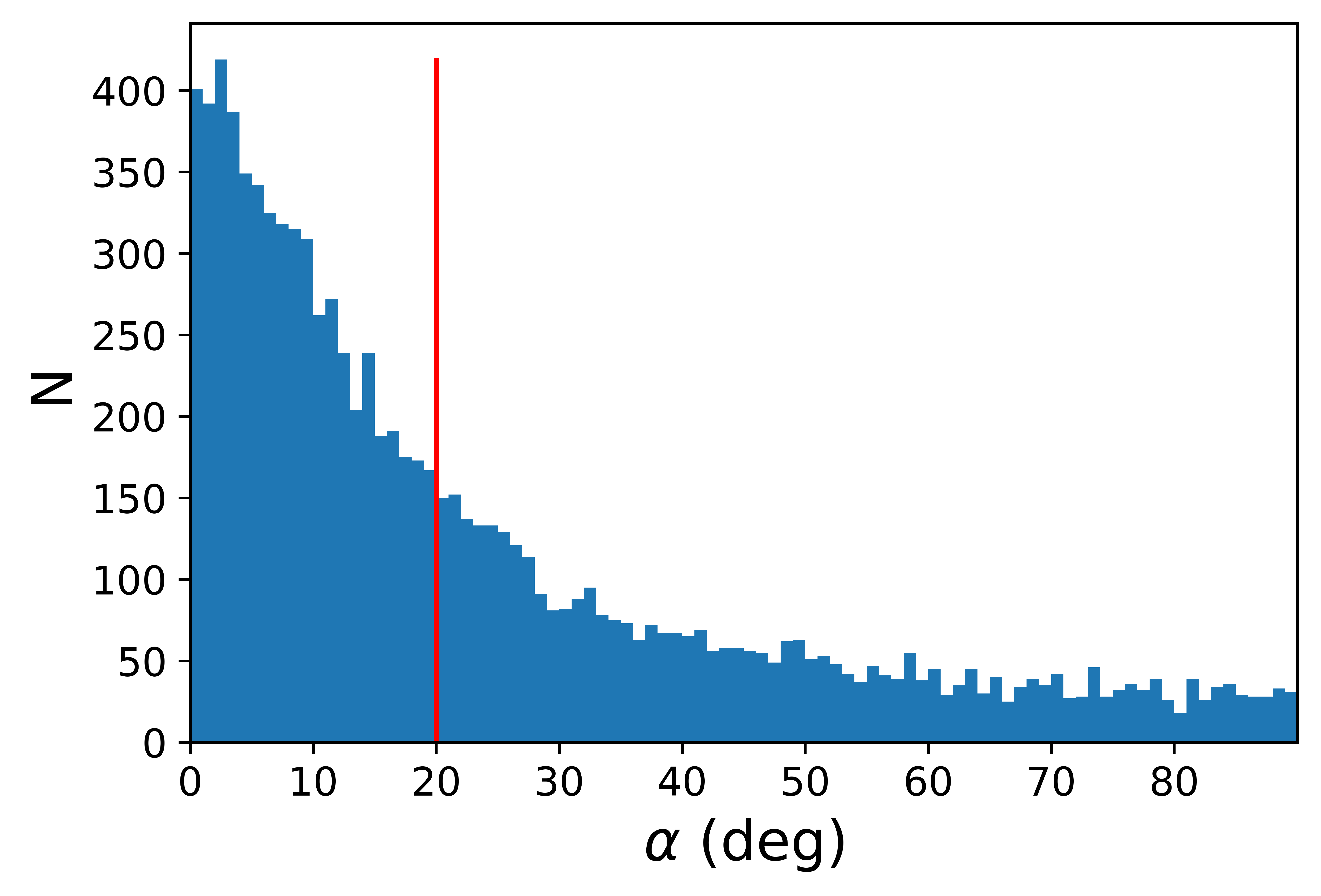
Figure 3: The histogram distribution of the phase-angle offset $\alpha$ of 9704 ”tails” with a ”head”. The red solid line refers to $\alpha=20^{\circ}$.

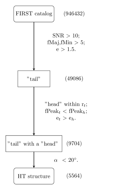
Figure 4: Flow chart of the procedure for the radio image identification. The total number in each catalog is labeled alongside its rectangle. The selection conditions are listed between the steps.

However, there are still many spurious sources showing HT-like patterns, e.g. parts of wide-angle tails, radio jets, small lobes, or even calibration artifacts. Fig.5 provides four cases to show this variety. J012132.4-095717 is an AGN with double jets because its optical counterparts (which will be checked later) are located in the middle of its head and tail. J114832.0+174723 passes our selection because of the contamination of calibration artifacts. J090018.1+074535 is part of a giant radio jet and there is a lobe on the opposite side, outside this figure. J113828.1+155450 is a part of a wide-angle tail structure.

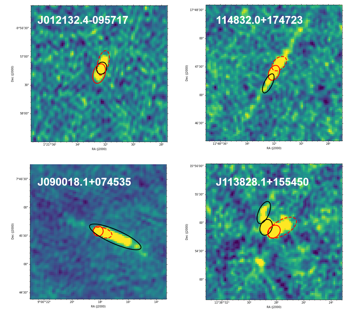
Figure 5: This figure shows four typical spurious sources showing HT-like patterns. All panels are show the same area of 2.4^′ $\times$ 2.4^′ and ellipses are Gaussian fittings from the FIRST catalog. Red solid ellipses refer to a “head” and red dashed ellipses mean “tail”. The white text label of each image is the FIRST ID of the “head” in the center. All these four structures satisfy our selection criteria, but they are not real OHT sources.

So it is difficult to identify OHTs with radio images alone. To select more reasonable candidates, we take optical images into account.

3 Optical Counterpart

The head of a real HT source coincides with its host galaxy, while the shape of the tail shows its trajectory on the sky plane. We cross-check our HT structures with the Sloan Digital Sky Survey (SDSS) data. We adopt the photometric catalog of SDSS DR12 (Alam et al., 2015). It covers 68% of the northern sky and about 90% of the FIRST area.

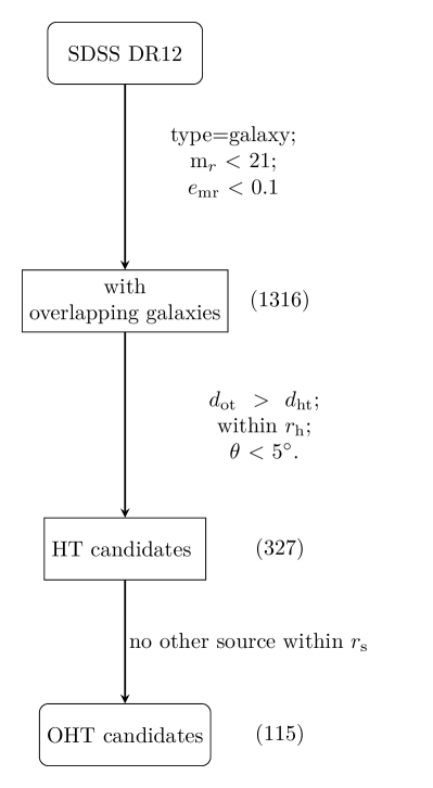
Figure 6: Flow chart of the procedure for the SDSS cross-checking. The total number of each catalog is labeled alongside its rectangle. The selection conditions are listed between the steps.

For each HT structure, we search for galaxies around its head in the SDSS photometric catalog. The automatic procedure of this section is illustrated by the flowchart Fig.6. There are 90% of 5564 HT structures that have optical objects within 3^′, but many of them are faint sources. To avoid unreliable faint sources, we only consider galaxies that are bright enough, that is to say, they have an r-band magnitude m_r $<$ 21 mag with an error $e_{mr}$ $<$ 0.1 mag. We then get 1316 galaxies corresponding with our HT structures.

Next, we select galaxies within a radius r_h = 1.5 times of the half major axis of the head (fMaj_h), and choose the closest one as the optical counterpart. In some cases, an optical galaxy is just located between the head and tail, as in the first case of Fig.5. This means both the head and the tail are actually jets of the galaxy. To filter off these cases, we add additional criteria: the distance between the optical galaxy and the tail (d_ot) should be larger than the distance between the head and the tail (d_ht), and the angle between the two lines $\theta$ should be less than 5 ^∘. So the optical galaxy will appear on the far end of the HT structure and align with the moving direction of the system. This illustration is given by Fig.7. The histogram distribution of $\theta$ is shown in Fig.8.

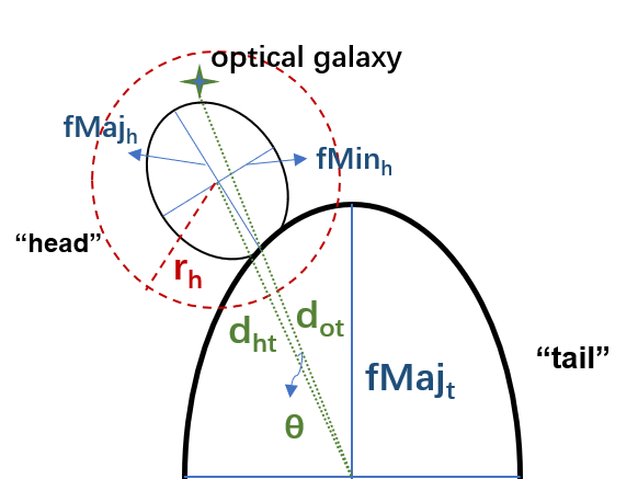
Figure 7: The red dashed circle r_h refers to the radius r_h = 1.5 times of the half major axis. The green star refers to the galaxy near the head. The two green dotted lines are the distance of head and tail with the galaxy and tail. $\theta$ is the angle between the two directions which must less than 5^∘ to make sure the galaxy aligns with the system.

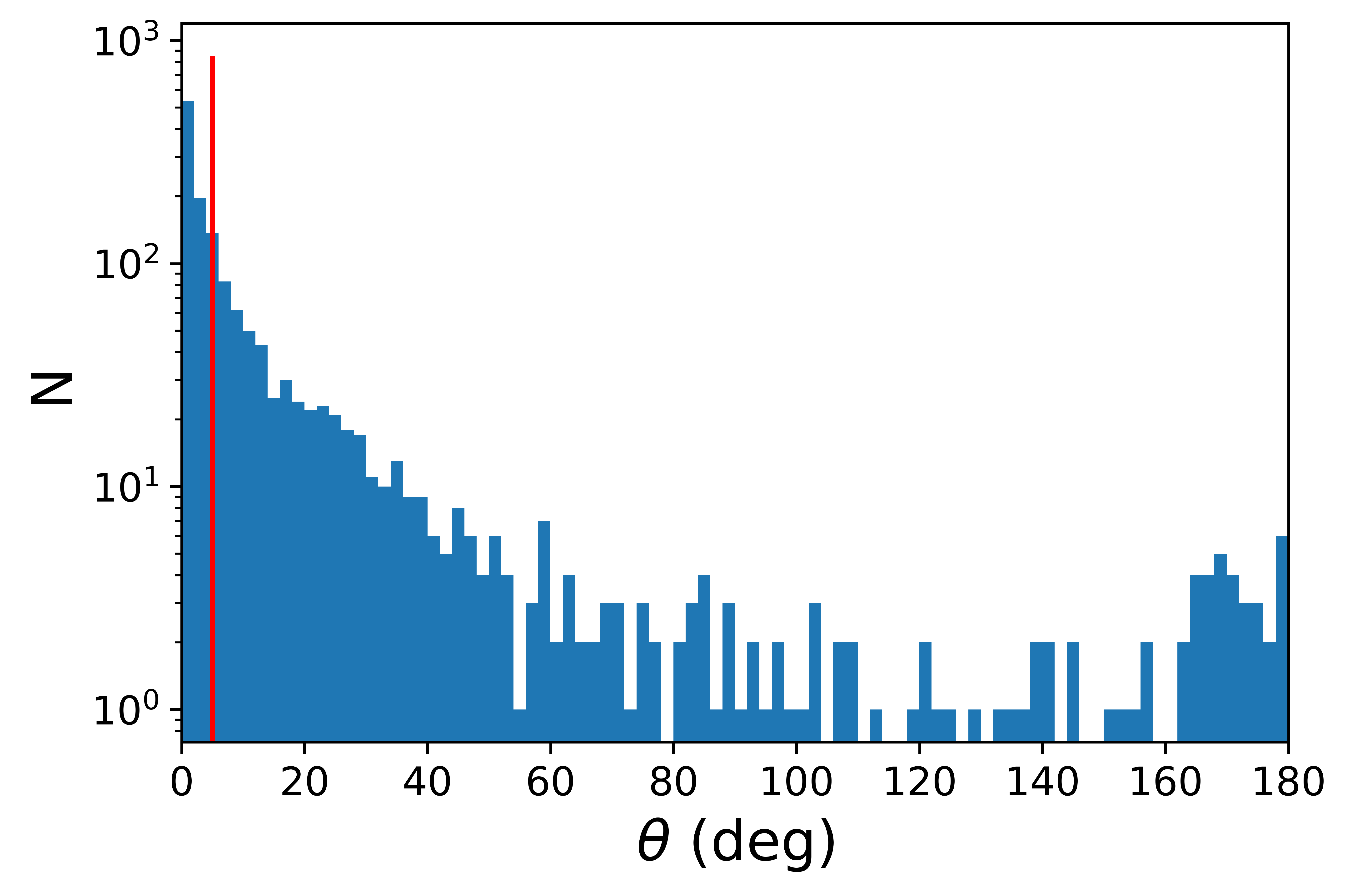
Figure 8: The histogram distribution of $\theta$ of 1316 galaxies and the red line refers to $\theta$ = 5^∘.

There are 327 galaxies satisfying all the above criteria. However, some of them are still a part of a double-jet radio galaxy, WAT galaxy, or NAT galaxy. We further add an isolation criterion: if there are any other radio sources except the tail and the head in the radius of the HT size $r_{s}=d_{ht}+fMaj_{t}$, we exclude the candidate. With this isolation criterion, we reduce our sample size to 115. The illustration is given by Fig.9.

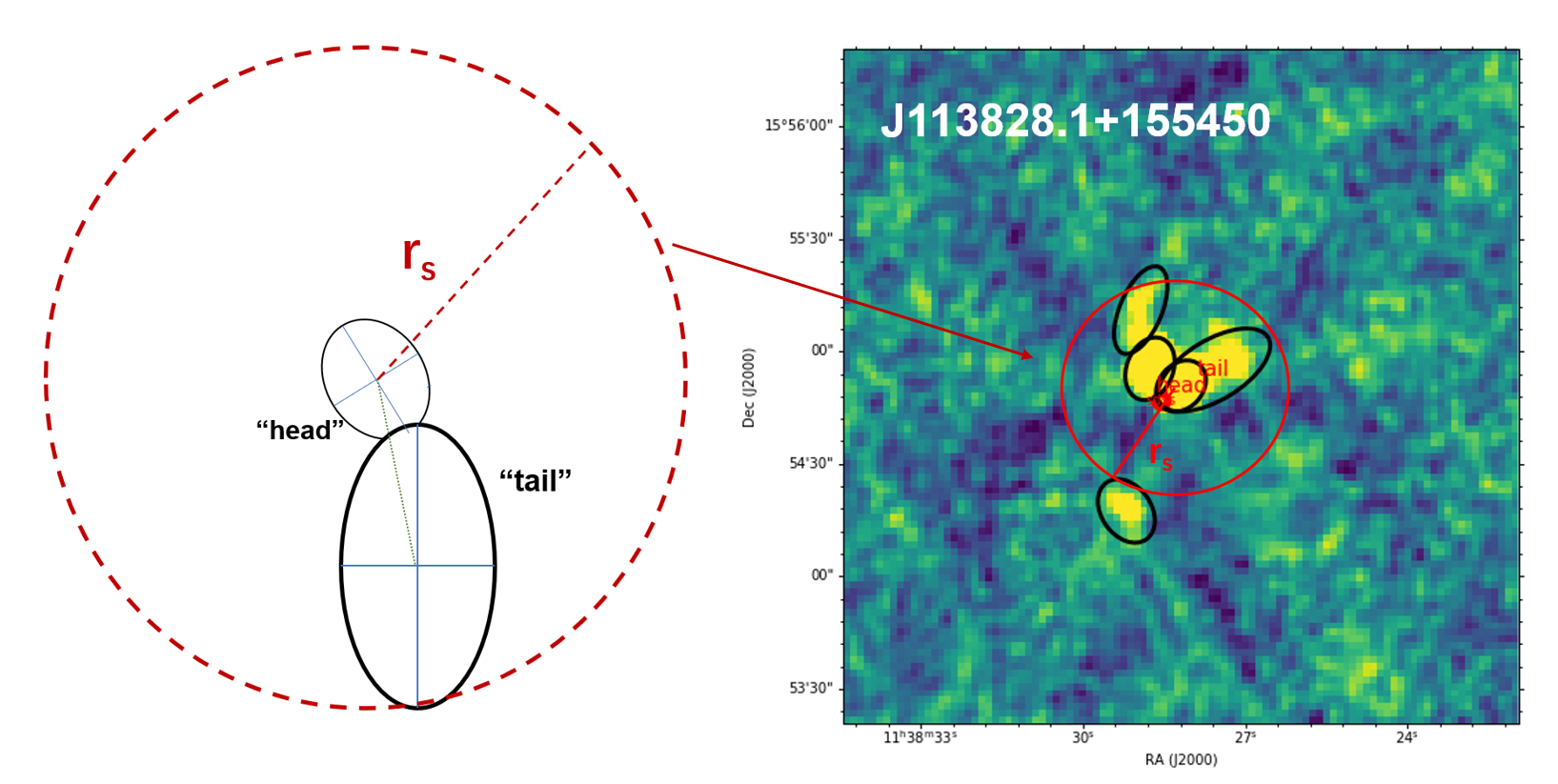
Figure 9: The red circle refers to the radius of the HT size r_s. We require there is no other source within r_s. J113828.1+155450 is a typical WAT. A part of it is selected as an OHT candidate. It is rejected by the isolation criterion.

Since the jets of some radio sources are separated a lot on the sky plane, beyond our checking radius r_s, there is no effective way to automatically identify them. We visually check our sample, and recognize another 21 jet components, 2 mergers, and 2 irregular patterns, and remove them. There are 90 isolated OHT candidates remaining in our catalog.

Additionally, there are three known OHT in the FIRST fields not recognized by our procedure. Both J134859.3+263334 in A1795 and J115508.8+232615 in A1413(Savini et al., 2019) are fitted with a single elongated Gaussian component. The third OHT is J134150.5+262217 in A1775(Terni de Gregory et al., 2017). It is rejected because of a nearby radio source belonging to the brightest central galaxy (BCG) of its host cluster. There are another two candidates found by chance—J084115.3 +075809 and J000313.1-060712. They are not selected by our procedure but noticed at the visual check stage. The former has a faint tail with a S/N of 7.6, smaller than our threshold of 10, while the latter is fitted with one Gaussian component. We add these five cases to our catalog manually, so the total number of candidates reaches 95.

There are 71 that have optical counterparts with spectroscopic measurements. For the rest, we adopt photometric redshifts (Alam et al., 2015). The peak fluxes and redshift distribution of these candidates are shown in Fig.10.

To estimate possible missing candidates likes the five sources mentioned above, we visually check 1000 fields selected randomly from 49,086 tail candidates. There are 138 radio HT structures found. The total number of HT structures can then reach to up 6774. Considering that only 115 out of 5564 HT structures pass all OHT checks, there will be about 140 OHT candidates that remain in the end. So we conclude that there might be about 18% (25 out of 140) OHT candidates that are missing when using our procedure.

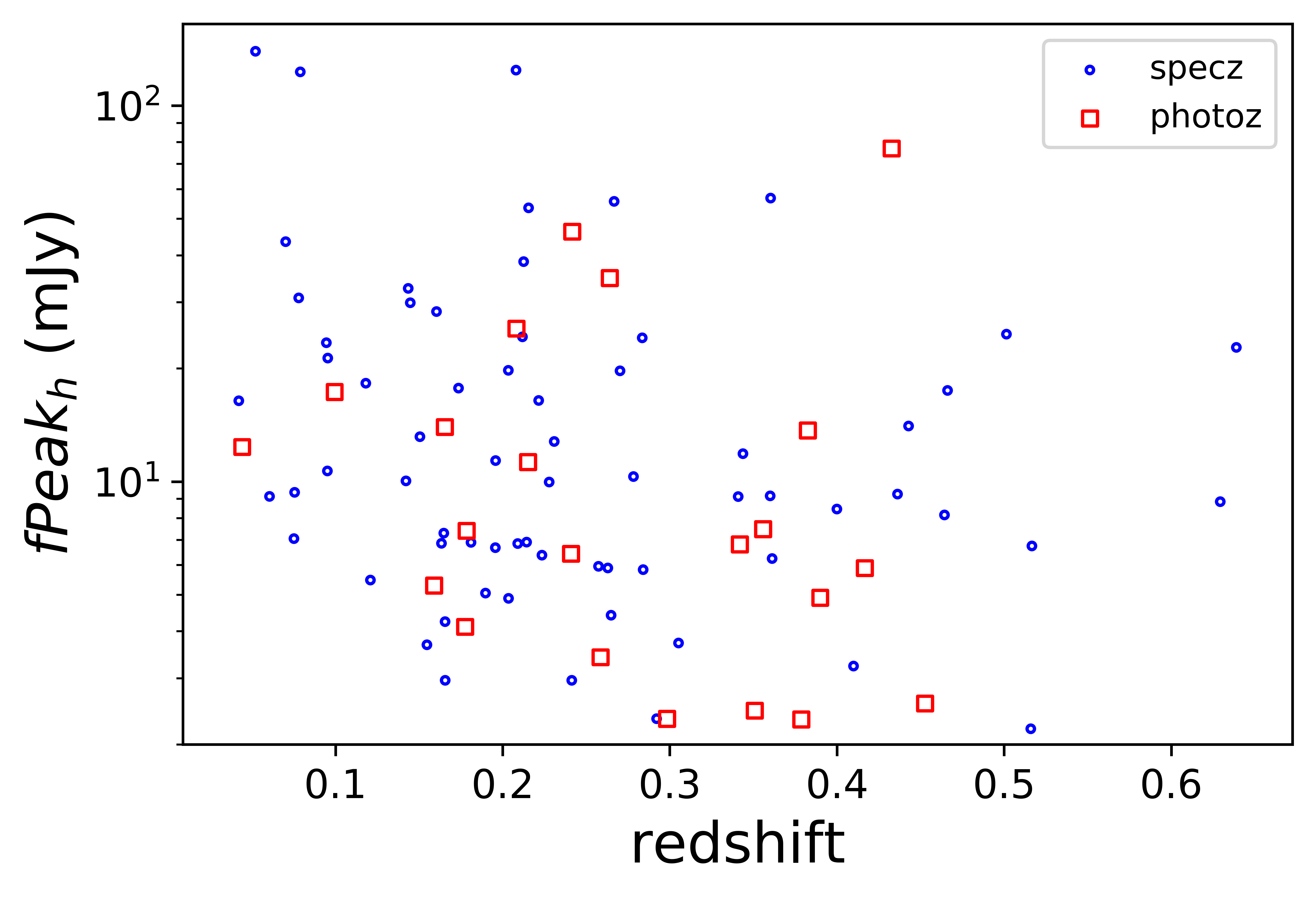
Figure 10: The peak fluxes of head and redshift distribution. Blue dots refer to galaxies with photometric redshifts while red dots refer to galaxies with spectroscopic redshifts.

4 cluster association

With some well-studied cases (Terni de Gregory et al., 2017), OHT structures are resolved as galaxies with high peculiar velocities located in the central region of clusters. Their two radio jets are bent as one along the opposite direction of their movement. But this scenario has only been verified in in few cases. With this new sample, we could verify this interpretation in a more general way.

We cross-check our OHT candidates with the Abell catalog (Abell et al., 1989) and cluster catalogs derived from the SDSS survey, e.g. the WHL2015 catalog (Wen & Han, 2015), the MSPM catalog (Smith et al., 2012), the SDSSCG catalog (McConnachie et al., 2009; Mendel et al., 2011), catalogs contained in the NASA/IPAC Extragalactic Database(NED; Mazzarella & NED Team, 2017) to search for possible host clusters around OHT candidates.

We check galaxy clusters within 1 ^∘ of each OHT candidate (r_s $<$ 1^∘ ). This radius corresponds to a projection distance of 6.7 Mpc at redshift 0.1, and 19.5 Mpc at redshift 0.4. We choose the closest cluster with a redshift difference smaller than 0.02 (Beck et al., 2016) as the association cluster. We then find association clusters for 89 out of 95 OHT candidates. All of the six sources without cluster association have relatively faint optical counterparts.

The histogram of the projected distance between isolated OHT candidates and association clusters is given by Fig.11. Sixty-five OHT candidates appear within 1 Mpc of association clusters. Twenty-six of them are located within a projected distance of 30 kpc, which is the typical size of elliptical galaxies(Das et al., 2010). Their host galaxies are more likely to be the central dominant (cD) galaxies of clusters. Since the cD galaxies could not have a large peculiar velocity, their tail-like structures might be parts of double jets. The opposite component on the other side is invisible due to the relativistic beaming effect(e.g. Sparks et al., 1992; Laing & Bridle, 2002), so we remove them and get 69 OHT galaxies in the end.

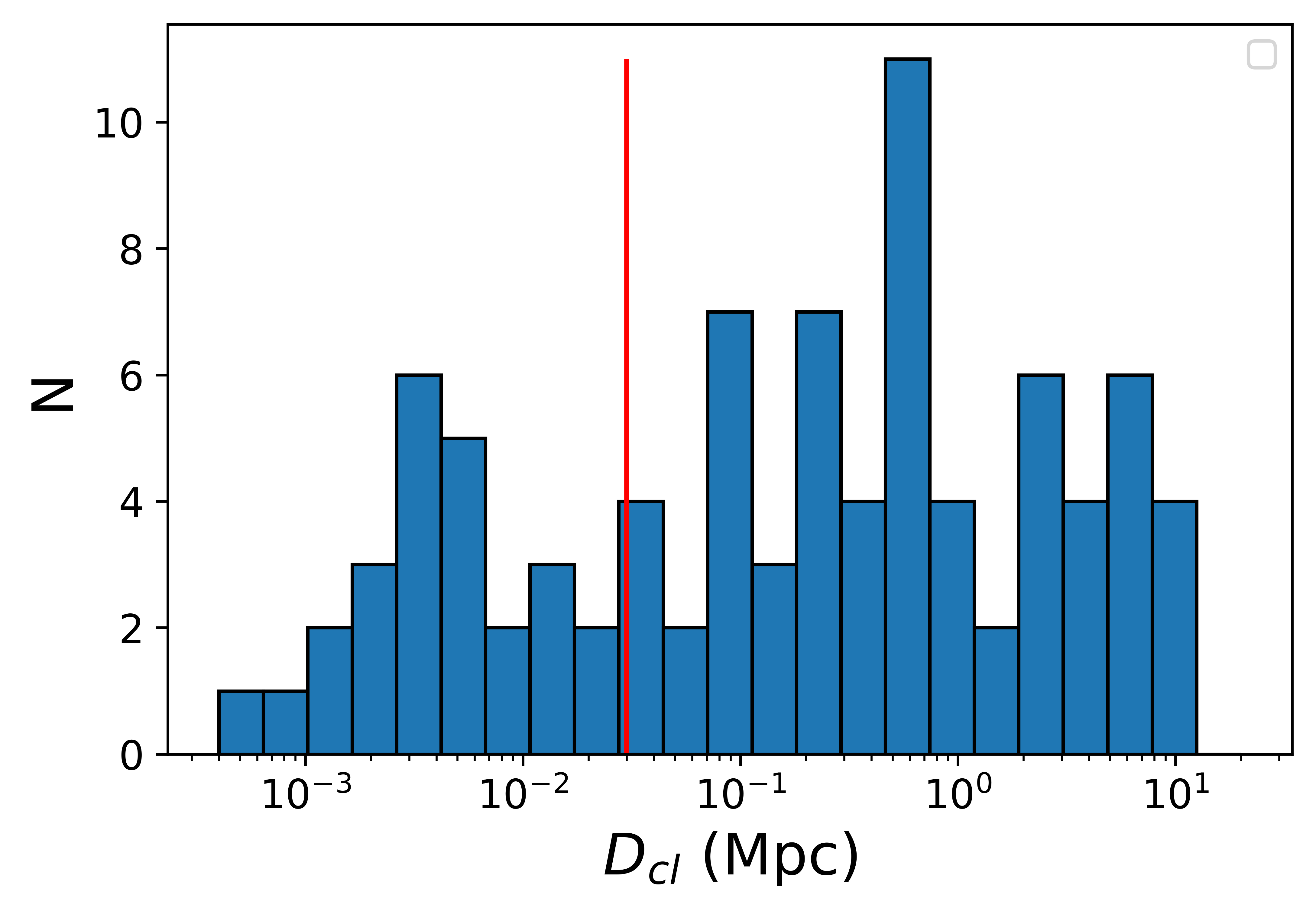
Figure 11: The distribution of projected distances between OHT candidates who have SDSS galaxy counterparts and the nearby galaxy clusters. The red solid line refers to 30 kpc, which is the typical size of elliptical galaxies(Das et al., 2010).

5 Sample properties

The basic properties of our OHT sample are listed in Table LABEL:tab:1. The first column is the serial number in our sample, the second column is the source id in the FIRST catalog, followed by the SDSS ID of its optical counterpart, the r-band magnitude, and the redshift. The sixth to eighth columns are the name of the association cluster, its redshift, and the projection distance between the head and the cluster center. There are six OHT candidates without cluster associations. Twenty-one host galaxies of OHT candidates have only photometric redshifts.

Table 1: When a spectroscopic redshift is not available, the SDSS photometric redshift is adopted instead, which is labeled with an asterisk (*).

	FIRST ID	SDSS ID	mr	zg	Cluster	zcl	Dcl
							(Mpc)
1	J000323.0-060458	1237672793959891057	17.62	0.241*	A2697	0.234	0.657
2	J004857.6+115641	1237678858476847541	19.68	0.390*	WHL J004906.0+115754	0.409*	0.790
3	J020159.9+034343	1237678660900421942	17.07	0.166	A293	0.165	0.217
4	J023834.4-032910	1237679255210623312	19.52	0.298*	WHL J023949.1-033022	0.317	5.245
5	J030013.1-051514	1237679439892643986	18.14	0.264*	WHL J030100.9-051223	0.266*	3.041
6	J035820.9+004223	1237666301633364230	19.30	0.383*	WHL J035820.6+003829	0.393*	1.266
7	J071130.2+390729	1237673429620032132	20.12	0.453*
8	J075357.7+420255	1237651192426004963	19.36	0.351*	WHL J075400.8+420246	0.367	0.183
9	J075431.9+164822	1237664835922100518	14.77	0.044*	MSPM 668	0.046*	0.033
10	J081859.7+494635	1237651272422522889	16.01	0.095	WHL J082041.5+492231	0.077	2.60
11	J085146.0+371440	1237657627901559004	18.31	0.178*	WHL J085146.2+371416	0.172	0.073
12	J085732.8+592751	1237663546906050701	17.28	0.203	WHL J085748.0+592925	0.203	0.502
13	J090327.1+042614	1237658423006396511	18.23	0.361	WHL J090429.6+040433	0.362	8.197
14	J091035.7+350741	1237664871895794181	19.84	0.516	WHL J091028.8+350836	0.519	0.641
15	J091327.7+555823	1237651191360586025	18.08	0.259*	WHL J091332.3+555857	0.269	0.211
16	J094613.8+022246	1237653665257357349	16.41	0.118	A869	0.120	0.105
17	J100623.5+240526	1237667293731684482	15.49	0.075	MSPM 6798	0.075*	0.471
18	J100850.4+135538	1237671260133065021	16.78	0.204	WHL J100840.4+135750	0.201	0.660
19	J102102.9+470055	1237658614124314722	17.35	0.181	WHL J102104.2+470054	0.179	0.041
20	J102604.0+390523	1237661138497896734	16.98	0.145	WHL J102622.9+390852	0.149	0.792
21	J104506.2+083718	1237671930671006606	20.79	0.639
22	J105624.7+164429	1237668585967714469	15.41	0.095	SDSSCGB 22800	0.095	0.074
23	J110532.0+073730	1237661972251213959	16.71	0.155	WHL J110527.0+073836	0.154	0.268
24	J111911.1+081538	1237661972789592202	15.02	0.076	MSPM 5279	0.075*	0.449
25	J112540.2+333924	1237665024363266295	19.06	0.356*
26	J114357.6+510236	1237657627916108093	20.56	0.501	WHL J114235.0+510545	0.501	4.967
27	J115716.8+333629	1237665126931234949	18.06	0.214	A1423	0.216	0.038
28	J122643.5+195050	1237667915421057112	16.97	0.224	WHL J122642.5+195026	0.222	0.104
29	J122902.4+473655	1237661357545095254	17.68	0.263	A1550	0.259	0.100
30	J123449.2+031136	1237651737371410669	18.87	0.410	WHL J123458.4+030449	0.409	2.371
31	J123547.4+030301	1237651754551083230	18.29	0.284	SDSSCGB 16587	0.284	0.045
32	J124042.3+020822	1237651753477931371	18.99	0.178*	XMMXCS J1243.0+0233	0.19	8.354
33	J124135.9+162033	1237668588651610193	15.04	0.070	MSPM 2617	0.071*	1.010
34	J125017.5+084215	1237658491211022497	18.61	0.342*	WHL J125019.9+084209	0.341	0.176
35	J125908.6+412937	1237662193992859752	17.89	0.278	WHL J125900.0+413128	0.277	0.629
36	J131525.2+171745	1237668624628842730	20.13	0.629
37	J132418.5+373531	1237664846122582252	17.74	0.241	WHL J132412.4+373334	0.240	0.533
38	J134436.7+534422	1237658802580226295	17.13	0.166	WHL J134456.3+534504	0.166	0.511
39	J135521.7-025453	1237655498129867111	19.12	0.165*	WHL J135522.7-031944	0.171*	5.02
40	J140412.9+562232	1237659144558281082	20.61	0.159*
41	J143258.5+291926	1237665101138952294	17.54	0.222	WHL J143321.8+292701	0.220	1.964
42	J144348.3-002601	1237648720711778680	18.29	0.305	WHL J144335.3-002106	0.292	1.569
43	J150746.8+040233	1237654880742277346	17.54	0.163	WHL J150813.6+042405	0.162	3.814
44	J150836.8+235224	1237665429713191101	17.01	0.196	WHL J150747.3+234533	0.196	2.615
45	J152045.1+483923	1237659163343716378	15.95	0.078	WHL J152052.2+483938	0.075	0.103
46	J152122.5+042030	1237662266464600297	13.86	0.052	MSPM 2944	0.052*	0.656
47	J153845.3-014018	1237655498678010865	19.94	0.417*	WHL J153845.6-013914	0.409*	0.357
48	J155618.5+213516	1237665127491567870	17.71	0.196	WHL J155615.3+213506	0.197	0.151
49	J155813.8+271621	1237662340012573171	16.37	0.095	A2142	0.091	0.278
50	J160149.7+490645	1237655349965750765	19.80	0.433*	MSPM 1271	0.432*	4.949
51	J161706.3+410646	1237665356696322197	17.73	0.267	WHL J161658.3+412836	0.285	5.713
52	J163802.7+162304	1237665231061648153	20.12	0.208*	WHL J163825.9+164018	0.181	3.348
53	J164021.9+464246	1237651715872325877	18.84	0.208	A2219	0.225	0.084
54	J164058.8+114404	1237665567159484554	14.96	0.078	WHL J163925.4+115131	0.085	2.329
55	J165250.6+630029	1237671767467754423	20.30	0.379*	WHL J165504.5+623409	0.372*	9.511
56	J172208.6+330640	1237665569838399705	15.83	0.099*	WHL J172216.4+330427	0.111	0.337
57	J210451.0+050320	1237669762788557036	18.54	0.242*	WHL J210322.5+051633	0.258*	6.242
58	J213319.1-063802	1237652936183185672	15.98	0.160	SDSSCGB 21196	0.160	3.071
59	J221807.6+085334	1237679009851441333	16.57	0.215*	WHL J221750.3+085544	0.234*	1.085
60	J224819.4-003641	1237666407360823478	17.33	0.213	WHL J224659.4-012817	0.206	11.338
61	J224830.6+122141	1237678860074615269	20.76	0.517
62	J231953.0-011625	1237653010821480629	17.84	0.284	WHL J231945.0-011729	0.287	0.593
63	J232437.2+143833	1237656242242060352	15.78	0.042	WHL J232420.1+143850	0.041	0.205
64	J232844.5+000134	1237663784193949861	17.48	0.292	WHL J232809.2+001109	0.278	3.342
65	J134859.3+263334	1237665532782838032	15.75	0.061	A1795	0.062	0.189
66	J115508.8+232615	1237667736653857373	20.64	0.194*	A1413	0.143	0.440
67	J134150.5+262217	1237665532245311533	14.42	0.069	A1775	0.072	0.060
68	J084115.3+075809	1237661066018488762	18.52	0.220*	WHL J084114.3+075844	0.245	0.146
69	J000313.1-060712	1237672793959891223	18.60	0.278*	A2697	0.232	0.465

To explore possible factors affecting the appearance of OHTs, we estimate the projected length of tails as $L_{tail}=(d_{ot}+fMaj_{t})D_{a}$, where $D_{a}$ is the angular diameter distance. We check the relationship between the tail length and the projected distance to the cluster center in Fig.12. The linear fitting result of 63 sources with cluster associations (in orange) is $L_{tail}/{\rm kpc}=(0.42\pm 2.73)D_{cl}/{\rm Mpc}+(113.53\pm 8.61)$. The shadow represents its 1$\sigma$ error range. We find no correlation between them.

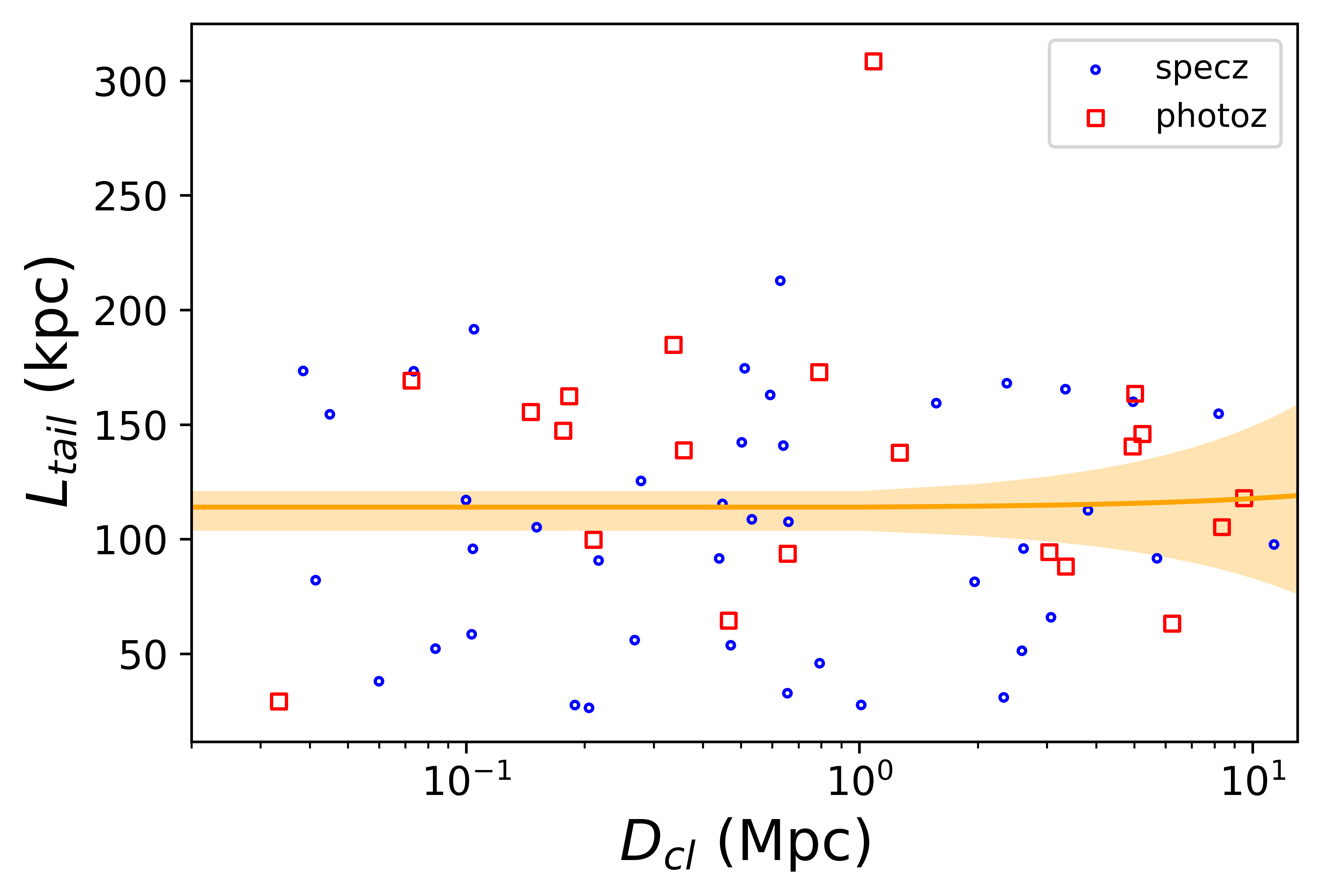
Figure 12: The scatter of projected distances to the cluster center D_cl and lengths of tails. Blue dots refer to the OHTs with spectroscopic redshifts, while the red squares refer to OHTs with photometric redshifts. The orange solid line is the linear fitting result of 63 sources with cluster associations $L_{tail}/{\rm kpc}=(0.42\pm 2.73)D_{cl}/{\rm Mpc}+(113.53\pm 8.61)$. The shadow represents its 1$\sigma$ error range.

With the richness of clusters (RL*) from the WHL2015 cluster catalog, the tail lengths does not show a clear correlation either (Fig.13). The orange solid line is the linear fitting result of 48 sources with WHL cluster richness, $L_{tail}/{\rm kpc}=(-0.92\pm 0.67)RL*+(131.68\pm 9.66)$. The weak anticorrelation suggests that long tails might trend to appear in poor clusters.

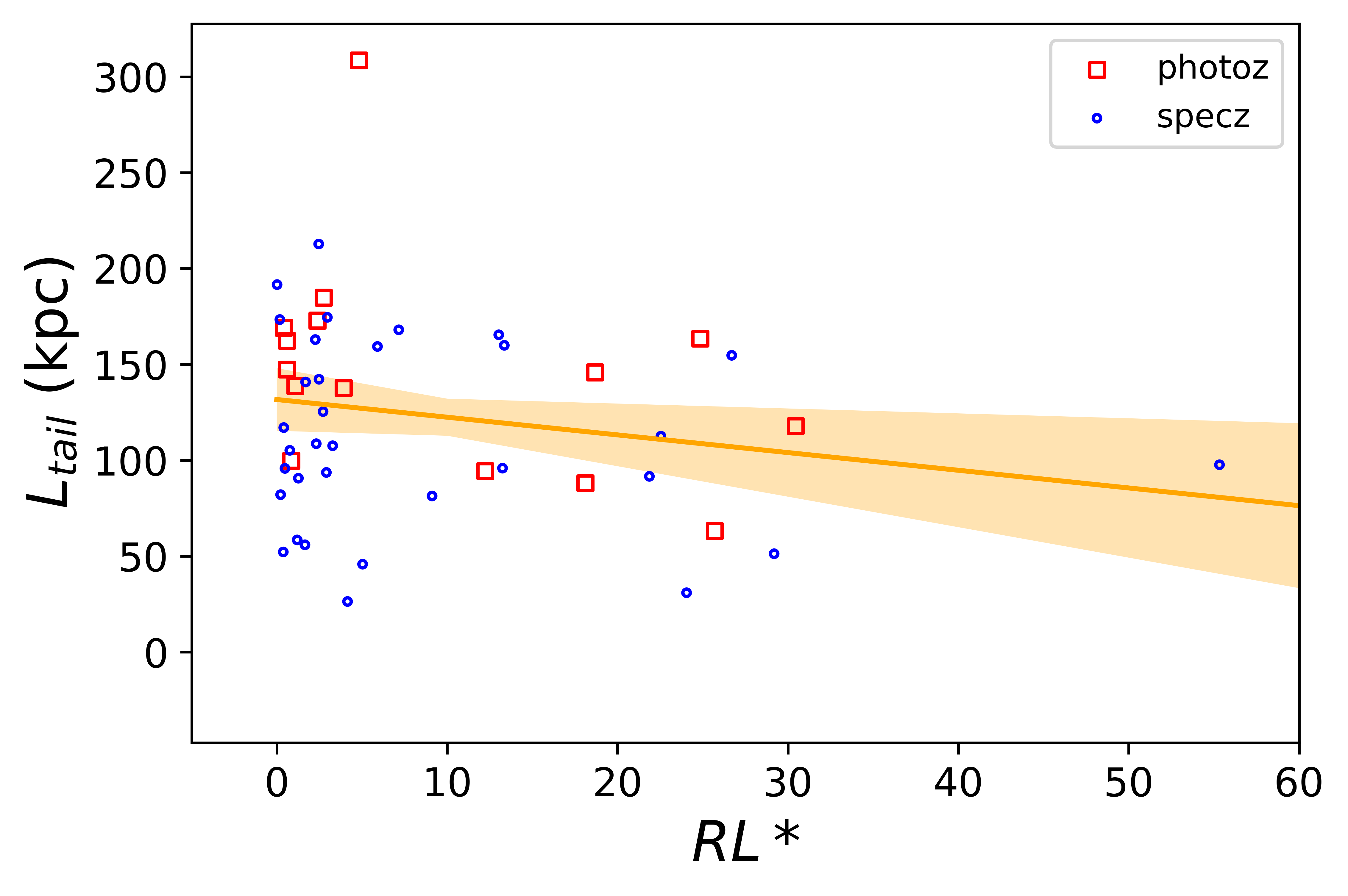
Figure 13: The scatter of the length of tail and richness of clusters using the WHL catalog. Blue dots refer to the OHTs with spectroscopic observation, while the red squares refer to OHTs with photometric redshifts. The orange solid line is the linear fitting result with 48 sources with WHL cluster richness, which is $L_{tail}/{\rm kpc}=(-0.92\pm 0.67)RL*+(131.68\pm 9.66)$. The shadow represents its 1$\sigma$ error range.

We also check the relationship between tail lengths and velocity differences between clusters and host galaxies c$\Delta$z as Fig.14 shows. Considering that precision of redshifts is crucial in this relationship, the linear fitting is only applied to 48 OHTs with spectroscopic redshifts. The result is $L_{tail}/{\rm kpc}=(-5.09\pm 5.51)c\Delta z/1000{\rm km~{}s^{-1}}+(111.53\pm 10.58)$. The weak anticorrelation we found is reasonable. Because the tail lengths of OHTs closely relate to the peculiar velocity of their host galaxies, the projected tail lengths observed are mainly dominated by the two velocity components projected on the sky plane. The redshift differences between galaxies and their host cluster are the radial velocity component. The larger it is, the less the other two are.

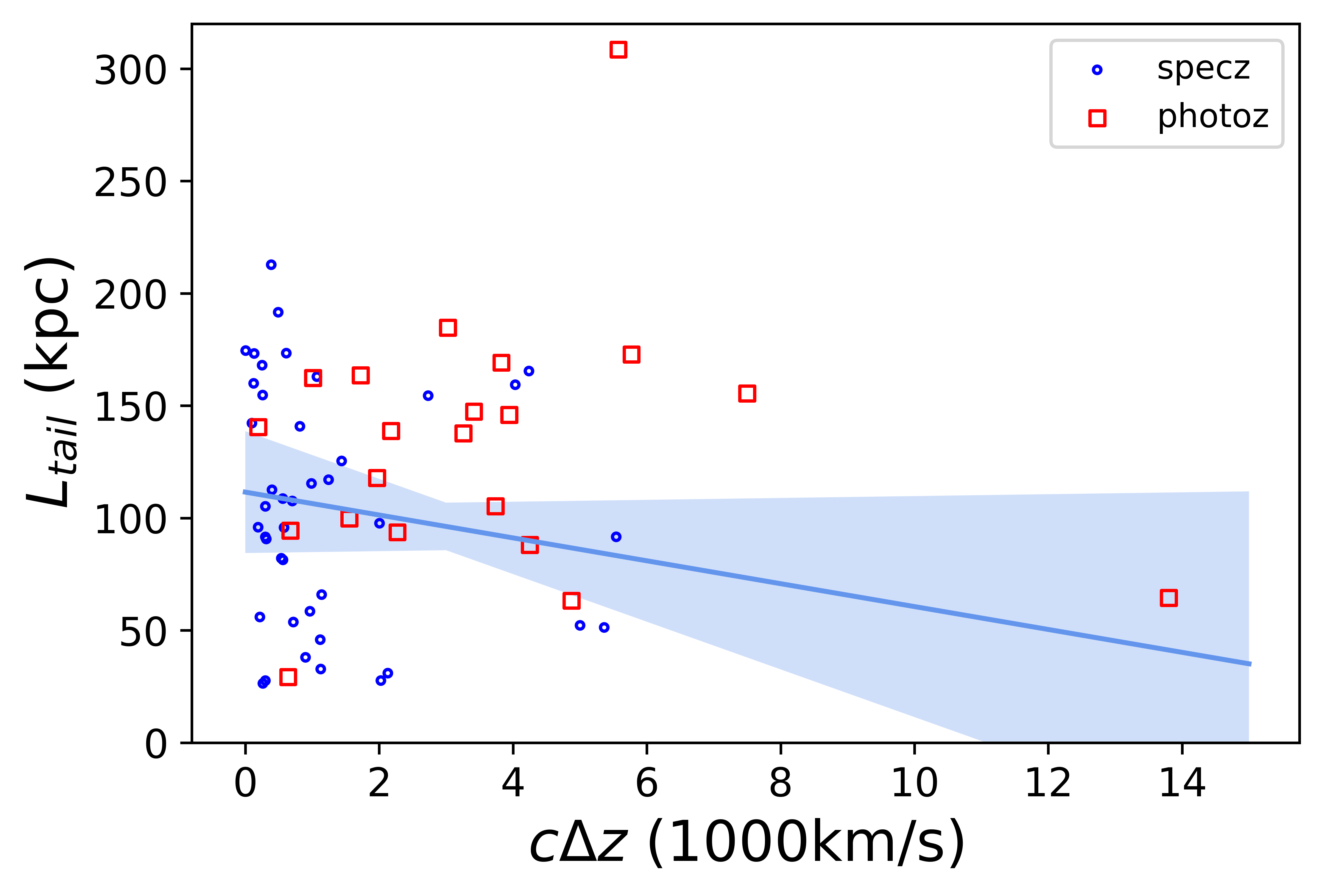
Figure 14: The scatter of tail lengths and velocity differences c$\Delta$z. Blue dots refer to OHTs with spectroscopic redshifts, while the red squares refer to OHTs that only have photometric redshifts. The blue solid line is the linear fitting result of 48 spectroscopic sources, which is $L_{tail}/{\rm kpc}=(-5.09\pm 5.51)c\Delta z/1000{\rm km~{}s^{-1}}+(111.53\pm 10.58)$. The shadow represents its 1$\sigma$ error range.

6 Discussion and Conclusions

We set up an automatic procedure to search for one-side head–tail structures in the FIRST survey catalog. It could identify OHT sources effectively, but there are still some sources, like NATs, WATs, one-sided jets, etc. showing a similar pattern. It is challenging to distinguish them with a radio image alone. After cross-checking with the SDSS photometric catalog and galaxy cluster catalogs, we compile an OHT catalog with 69 sources. Most of them have not been noticed before. As the first OHT catalog, our sample provides a fair data set for future deep-radio and optical observations. Details of these comprehensive OHT sources will be helpful for understanding their occurrence and properties. This catalog could also be taken as a training sample of machine-learning applications to find more examples in a future radio survey.

We also notice that Gaussian components in the FIRST catalog do not always provide a good morphological description of radio sources. With a modern fitting procedure like PyBDSF(Mohan & Rafferty, 2015), the source list could describe extended emission better, and the performance of our procedure could then be further improved. A example case, J004013.5+012546, is given by Fig.15. It is one of the 115 OHT candidates but is recognized as a jet lobe by the visual check, then dropped. Its central part shows an HT-like structure in the FIRST fitting result (left panel), while the PyBDSF fitting regions (right panel) give a more reasonable estimate. However, updating the whole FIRST catalog with the new fitting procedure is beyond the goal of this paper.

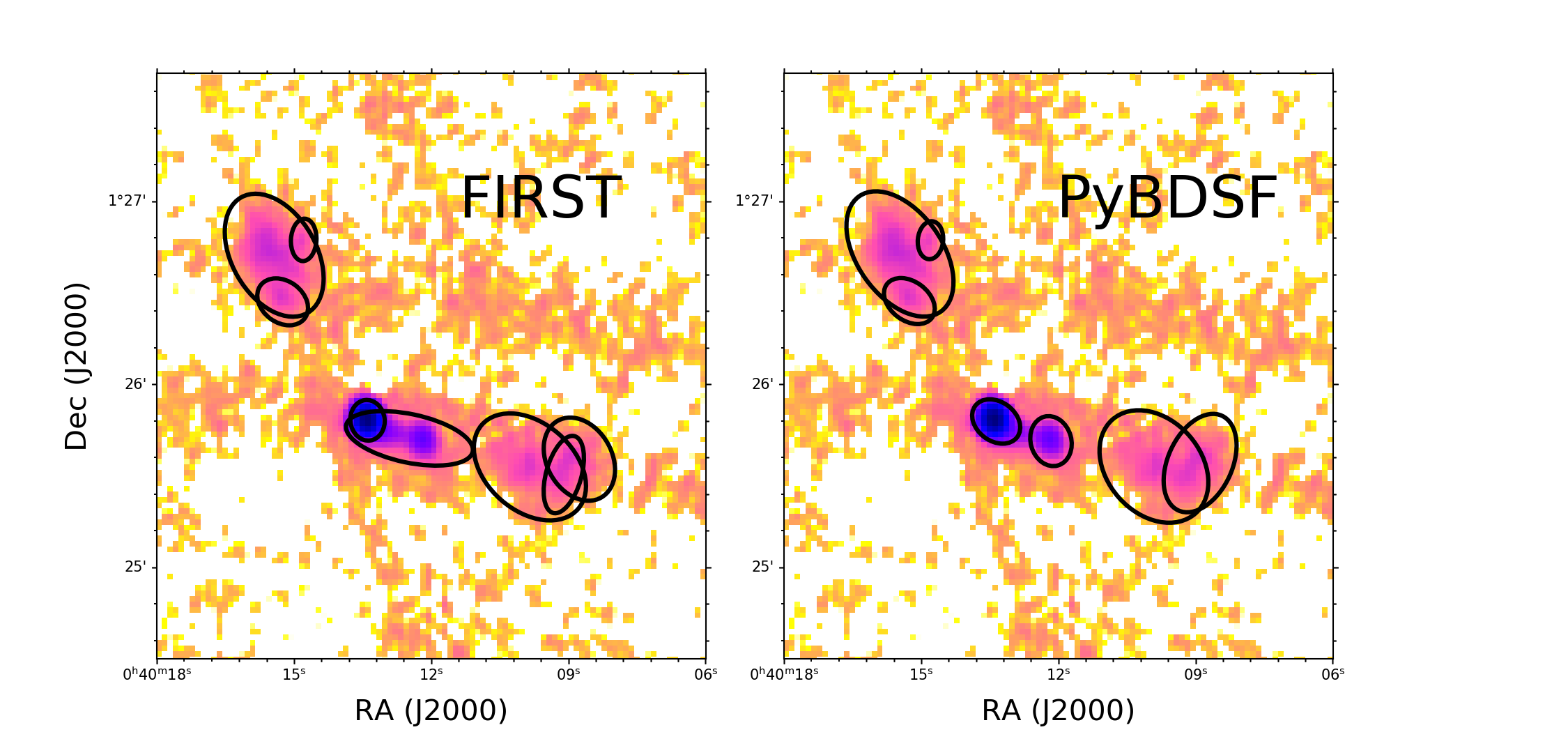
Figure 15: The comparison of Gaussian components in FIRST catalog (left panel) and fitting by PyBDSF (right panel) in the same field of J004013.5+012546, which is one of the 115 OHT candidates but is dropped by the visual check. Each panel is in the size 3^′ $\times$ 3^′.

With this sample, we confirm that most OHTs are in the gravitational potential wells of clusters. The lengths of their tails do not correlate with the projection distance to the center of the nearest galaxy clusters. But they show weak anticorrelation with the cluster richness, and are inversely proportional to the radial velocity differences between clusters and host galaxies. There are still some sources that are in the outskirts of clusters or even fully outside known clusters. Further radio observations with high angular resolution and spectral maps are necessary to reveal more details.

Upcoming radio surveys, like the LoTSS (Shimwell et al., 2017), the Australian Square Kilometre Array Pathfinder survey(Johnston et al., 2007), the Jansky VLA Sky Survey (Lacy et al., 2020), and the Square Kilometer Array (https://www.skatelescope.org/) will discover more HT sources and provide better chances to study and understand this special type of radio galaxies.

Appendix A identification charts of OHT candidates

To show the morphology of OHT candidates, we list identification charts of all 69 sources in our sample. The radio contours overlap on top of SDSS r-band images. The ellipses on the map represent source shapes from the FIRST catalog. The recognized heads and tails are labeled with a small “h” and “t” correspondingly. With identification charts, we can compare radio morphologies and FIRST fitting results directly, and check if assigned optical counterparts are chance alignments. With these images, we confirm that our procedure of OHT identification is generally consistent with the visual check.

Table 2: Identification charts of all 69 OHT candidates. The radio contour maps overlap on top of SDSS r-band images. All images are in the same size 1.8^′ $\times$ 1.8^′. The radio contours use the ”hot” colormap. The title of each images is the FIRST ID of the “head” in the center. The blue ellipses on the map represent source shapes from the FIRST catalog. The recognized heads and tails are labelled with the small red “h” and “t” correspondingly.

1	2	3	4
5	6	7	8
9	10	11	12
13	14	15	16
17	18	19	20
21	22	23	24
25	26	27	28
29	30	31	32
33	34	35	36
37	38	39	40
41	42	43	44
45	46	47	48
49	50	51	52
53	54	55	56
57	58	59	60
61	62	63	64
65	66	67	68
69

References

- Abell et al. (1989) Abell, G. O., Corwin, Harold G., J., & Olowin, R. P. 1989, ApJS, 70, 1
- Alam et al. (2015) Alam, S., Albareti, F. D., Allende Prieto, C., et al. 2015, ApJS, 219, 12
- Banfield et al. (2015) Banfield, J. K., Wong, O. I., Willett, K. W., et al. 2015, MNRAS, 453, 2326
- Beck et al. (2016) Beck, R., Dobos, L., Budavári, T., Szalay, A. S., & Csabai, I. 2016, MNRAS, 460, 1371
- Becker et al. (1995) Becker, R. H., White, R. L., & Helfand, D. J. 1995, ApJ, 450, 559
- Condon et al. (1998) Condon, J. J., Cotton, W. D., Greisen, E. W., et al. 1998, AJ, 115, 1693
- Das et al. (2010) Das, P., Gerhard, O., Churazov, E., & Zhuravleva, I. 2010, MNRAS, 409, 1362
- Feretti & Giovannini (2008) Feretti, L., & Giovannini, G. 2008, Clusters of Galaxies in the Radio: Relativistic Plasma and ICM/Radio Galaxy Interaction Processes, ed. M. Plionis, O. López-Cruz, & D. Hughes, Vol. 740, 24
- Garon et al. (2019) Garon, A. F., Rudnick, L., Wong, O. I., et al. 2019, AJ, 157, 126
- Intema et al. (2017) Intema, H. T., Jagannathan, P., Mooley, K. P., & Frail, D. A. 2017, A&A, 598, A78
- Johnston et al. (2007) Johnston, S., Bailes, M., Bartel, N., et al. 2007, PASA, 24, 174
- Jones & McAdam (1996) Jones, P. A., & McAdam, W. B. 1996, MNRAS, 282, 137
- Lacy et al. (2020) Lacy, M., Baum, S. A., Chandler, C. J., et al. 2020, PASP, 132, 035001
- Laing & Bridle (2002) Laing, R. A., & Bridle, A. H. 2002, MNRAS, 336, 328
- Mao et al. (2009) Mao, M. Y., Johnston-Hollitt, M., Stevens, J. B., & Wotherspoon, S. J. 2009, MNRAS, 392, 1070
- Mazzarella & NED Team (2017) Mazzarella, J. M., & NED Team. 2017, in Astroinformatics, ed. M. Brescia, S. G. Djorgovski, E. D. Feigelson, G. Longo, & S. Cavuoti, Vol. 325, 379–384
- McConnachie et al. (2009) McConnachie, A. W., Patton, D. R., Ellison, S. L., & Simard, L. 2009, MNRAS, 395, 255
- Mendel et al. (2011) Mendel, J. T., Ellison, S. L., Simard, L., Patton, D. R., & McConnachie, A. W. 2011, MNRAS, 418, 1409
- Miley (1980) Miley, G. 1980, ARA&A, 18, 165
- Miley et al. (1972) Miley, G. K., Perola, G. C., van der Kruit, P. C., & van der Laan, H. 1972, Nature, 237, 269
- Miraghaei & Best (2017) Miraghaei, H., & Best, P. N. 2017, MNRAS, 466, 4346
- Mohan & Rafferty (2015) Mohan, N., & Rafferty, D. 2015, PyBDSF: Python Blob Detection and Source Finder, , , ascl:1502.007
- O’Neill et al. (2019) O’Neill, B. J., Jones, T. W., Nolting, C., & Mendygral, P. J. 2019, ApJ, 887, 26
- Pratley et al. (2013) Pratley, L., Johnston-Hollitt, M., Dehghan, S., & Sun, M. 2013, MNRAS, 432, 243
- Proctor (2011) Proctor, D. D. 2011, ApJS, 194, 31
- Ryle & Windram (1968) Ryle, M., & Windram, M. D. 1968, MNRAS, 138, 1
- Savini et al. (2019) Savini, F., Bonafede, A., Brüggen, M., et al. 2019, A&A, 622, A24
- Shimwell et al. (2017) Shimwell, T. W., Röttgering, H. J. A., Best, P. N., et al. 2017, A&A, 598, A104
- Shimwell et al. (2019) Shimwell, T. W., Tasse, C., Hardcastle, M. J., et al. 2019, A&A, 622, A1
- Smith et al. (2012) Smith, A. G., Hopkins, A. M., Hunstead, R. W., & Pimbblet, K. A. 2012, MNRAS, 422, 25
- Sparks et al. (1992) Sparks, W. B., Fraix-Burnet, D., Macchetto, F., & Owen, F. N. 1992, Nature, 355, 804
- Srivastava & Singal (2020) Srivastava, S., & Singal, A. K. 2020, MNRAS, 493, 3811
- Terni de Gregory et al. (2017) Terni de Gregory, B., Feretti, L., Giovannini, G., et al. 2017, A&A, 608, A58
- Wen & Han (2015) Wen, Z. L., & Han, J. L. 2015, ApJ, 807, 178
- White et al. (1997) White, R. L., Becker, R. H., Helfand, D. J., & Gregg, M. D. 1997, ApJ, 475, 479
- Yu et al. (2018) Yu, H., Tozzi, P., van Weeren, R., et al. 2018, ApJ, 853, 100