Explicit Convergence Rates of Greedy and Random Quasi-Newton Methods

Abstract

Optimization is important in machine learning problems, and quasi-Newton methods have a reputation as the most efficient numerical methods for smooth unconstrained optimization. In this paper, we study the explicit superlinear convergence rates of quasi-Newton methods and address two open problems mentioned by Rodomanov and Nesterov (2021b). First, we extend Rodomanov and Nesterov (2021b)’s results to random quasi-Newton methods, which include common DFP, BFGS, SR1 methods. Such random methods employ a random direction for updating the approximate Hessian matrix in each iteration. Second, we focus on the specific quasi-Newton methods: SR1 and BFGS methods. We provide improved versions of greedy and random methods with provable better explicit (local) superlinear convergence rates. Our analysis is closely related to the approximation of a given Hessian matrix, unconstrained quadratic objective, as well as the general strongly convex, smooth, and strongly self-concordant functions.

Keywords: quasi-Newton methods, superlinear convergence, local convergence, rate of convergence, Broyden family, SR1, BFGS, DFP

1 Introduction

Many machine learning problems can be formulated to the minimization of an objective defined as the expectation over a set of random functions (Liu and Nocedal, 1989; Bottou and Le Cun, 2005; Shalev-Shwartz and Srebro, 2008; Mokhtari and Ribeiro, 2014, 2015). Specifically, given the training sample ${\bm{z}}\sim{\mathcal{D}}$, where ${\mathcal{D}}$ is the data distribution, we consider an optimization function $f:{\mathbb{R}}^{d}\to{\mathbb{R}}$:

$$\min_{{\bm{x}}\in{\mathbb{R}}^{d}}f({\bm{x}})=\mathbb{E}_{{\bm{z}}\sim{\mathcal{D}}}\;\ell({\bm{x}},{\bm{z}})+R({\bm{x}}),$$

where $\ell({\bm{x}},{\bm{z}})$ is the loss with respect to the training sample ${\bm{z}}$, and $R({\bm{x}})$ is some regularization function, such as $\left\|{\bm{x}}\right\|^{2}_{2}$. When ${\mathcal{D}}$ is the empirical distribution of training samples $\{{\bm{z}}_{i}\}_{i=1}^{n}$, we could recover the classical finite-sum empirical risk minimization:

$$\min_{{\bm{x}}\in{\mathbb{R}}^{d}}f({\bm{x}})=\frac{1}{n}\sum_{i=1}^{n}\ell({\bm{x}},{\bm{z}}_{i})+R({\bm{x}}).$$

Such a finite-sum formulation encapsulates a wide variety of machine learning problems including least squares regression, support vector machines (SVM), logistic regression, neural networks, and graphical models.

Previous methods mainly use first-order methods by evaluating objective function gradients $\nabla f({\bm{x}})$, such as gradient descent, stochastic gradient descent, accelerated gradient descent (Nesterov, 2003), Adagrad (Duchi et al., 2011), Adam (Kingma and Ba, 2015), etc. These methods dominate the current optimization methods of machine learning problems, and have affordable computation complexity in each iteration. However, these first-order methods generally only have a linear or sublinear convergence rate even if the objective has nice properties.

Recently, second-order methods have also received great attention due to their fast convergence rates compared to first-order methods. But second-order methods, such as Newton’s method, are impractical because the exact Hessian matrix $\nabla^{2}f({\bm{x}})$ needs high computation cost in general cases. Common wisdom proposes quasi-Newton methods by replacing Hessian matrices with some reasonable approximations. The approximation is updated in iterations based on some special formulas from the previous variation.

Quasi-Newton methods have a broad application in machine learning problems (Bordes et al., 2009; Yu et al., 2010; Mokhtari and Ribeiro, 2015; Yuan and Li, 2020; Ye et al., 2020; Liu and Owen, 2021). There exist various quasi-Newton algorithms with different Hessian approximations. The three most popular versions are the Davidon-Fletcher-Powell (DFP) method (Fletcher and Powell, 1963; Davidon, 1991), the Broyden-Fletcher-Goldfarb-Shanno (BFGS) method (Broyden, 1970a, b; Fletcher, 1970; Goldfarb, 1970; Shanno, 1970), and the Symmetric Rank 1 (SR1) method (Broyden, 1967; Davidon, 1991), all of which belong to the Broyden family (Broyden, 1967) of quasi-Newton algorithms. The most attractive property of quasi-Newton methods compared to the classical first-order methods, is their superlinear convergence, which can trace back to the 1970s (Powell, 1971; Broyden et al., 1973; Dennis and Moré, 1974). However, the superlinear convergence rates provided in prior work are asymptotic (Stachurski, 1981; Griewank and Toint, 1982; Byrd et al., 1987; Yabe and Yamaki, 1996; Kovalev et al., 2020). The results only show that the ratio of successive residuals tends to zero as the running iterations approach to infinity, i.e.,

$$\lim_{k\to+\infty}\frac{\left\|{\bm{x}}_{k+1}-{\bm{x}}_{*}\right\|}{\left\|{\bm{x}}_{k}-{\bm{x}}_{*}\right\|}=0,\text{ or }\left\|{\bm{x}}_{k+1}-{\bm{x}}_{*}\right\|=o(\left\|{\bm{x}}_{k}-{\bm{x}}_{*}\right\|),$$

where $\{{\bm{x}}_{k}\}$ is iterative update sequence, $k$ is the iteration counter, and ${\bm{x}}_{*}$ is the optimal solution. It is unknown whether the residuals converge like $O(c^{k^{2}}),O(k^{-k})$, where $c\in(0,1)$ is some constant. Hence, the theory is inadequate and there still lacks of a specific superlinear convergence rate. Additionally, machine learning problems have requirement of the explicit convergence rates to compare the performance and design better algorithms for applications. Therefore, to give a better guidance of quasi-Newton methods in machine learning problems, we are still interested in the explicit rates of quasi-Newton methods.

Recently, Rodomanov and Nesterov (2021b) gave the first explicit local superlinear convergence for their proposed new quasi-Newton methods. They introduced greedy quasi-Newton updates by greedily selecting from basis vectors to maximize a certain measure of progress, and established an explicit non-asymptotic bound on the local superlinear convergence rate correspondingly. However, as Rodomanov and Nesterov (2021b) stated, “greedy methods require additional information beyond just the gradient of the objective function.” A natural idea might be to replace the greedy strategy with a randomized one. Indeed, the strategy of randomness has almost the same performance as the greedy one, which has been observed in Rodomanov and Nesterov (2021b)’s experiments. Therefore, one can expect that it should be possible to establish similar theoretical results about its superlinear convergence, but they did not provide theoretical guarantees. This raises the issue: can we give explicit superlinear rates for random quasi-Newton methods theoretically? In addition, Rodomanov and Nesterov (2021b)’s proofs are mainly applicable to the DFP methods because they reduced all possible Broyden family to the DFP update based on the monotonicity property (see Lemma 5). However, the SR1 and BFGS updates are more popular and faster than the DFP update in practice, which also has been verified in their experiments. Thus, it is natural to ask can we obtain separate superlinear rates for different quasi-Newton methods?

In this work, we solve the above two problems rigorously. We extend Rodomanov and Nesterov (2021b)’s results into random quasi-Newton methods, and improve the local superlinear convergence rates by our revised greedy or random SR1 and BFGS methods. We present our contribution in detail as follows:

• First, we extend Rodomanov and Nesterov (2021b)’s results to random quasi-Newton methods, which use a random direction for updating the approximate Hessian matrix. Our superlinear convergence rate is of the form $(1-\frac{1}{d\varkappa+1})^{k(k-1)/2}$ with high probability, which is similar as the greedy-type methods proposed by Rodomanov and Nesterov (2021b, Theorem 4.9). Here, $\varkappa$ is the condition number of the objective function, $k$ is the current iteration, and $d$ is the dimension of parameters.

• Second, for specific quasi-Newton methods, including SR1 and BFGS methods, we provide improved versions of greedy and random methods. We show that for approximating a fixed Hessian matrix, both the methods share a faster condition-number-free convergence. Particularly, we can obtain the superlinear convergence rate $O((1{-}\frac{k}{d})_{+})$ for the SR1 update, and the linear convergence rate $O((1{-}\frac{1}{d})^{k})$ for the BFGS update, where $(x)_{+}=\max\{x,0\}$. Both the findings improve the original convergence rate $O((1{-}\frac{1}{d\varkappa})^{k})$ by Rodomanov and Nesterov (2021b, Theorem 2.5).

• Third, we extend our analysis to a practical scheme, showing (local) superlinear convergence under our proposed greedy/random SR1 and BFGS update, when applied to unconstrained quadratic objective or strongly self-concordant functions. We list our results in Table 1 with the same formulation as the work of Rodomanov and Nesterov (2021b). Note that in general, the convergence goes through two phases. The first phase lasts for $k_{0}$ iterations, and only has a linear convergence rate $O((1{-}\frac{1}{2\varkappa})^{k_{0}})$. The second phase has a superlinear convergence rate $O((1{-}\frac{1}{d})^{k(k-1)/2})$. Our revised bound takes fewer first-phase iterations $k_{0}$ as well as a faster (condition-number-free) superlinear convergence rate in the second phase compared to Rodomanov and Nesterov (2021b)’s results.

Quasi-Newton Methods	Superlinear Rates	$k_{0}$
Greedy Broyden Rodomanov and Nesterov (2021b)	$\left(1-\frac{1}{d\varkappa}\right)^{k(k-1)/2}\left(\frac{1}{2}\right)^{k}\!\left(1{-}\frac{1}{2\varkappa}\right)^{k_{0}}$	$O\left(d\varkappa\ln(d\varkappa)\right)$
Random Broyden (Corollary 12)	$\big{(}1{-}\frac{1}{d\varkappa{+}1}\big{)}^{k(k{-}1)/2}\left(\frac{1}{2}\right)^{k}\!\left(1{-}\frac{1}{2\varkappa}\right)^{k_{0}}$	$O\left(d\varkappa\ln(d\varkappa/\delta)\right)$
Greedy BFGS*/SR1 (Corollary 20)	$\left(1-\frac{1}{d}\right)^{k(k-1)/2}\left(\frac{1}{2}\right)^{k}\!\left(1{-}\frac{1}{2\varkappa}\right)^{k_{0}}$	$O\left(\left(d+\varkappa\right)\ln(d\varkappa)\right)$
Random BFGS/SR1 (Corollary 20)	$\big{(}1{-}\frac{1}{d+1}\big{)}^{k(k-1)/2}\left(\frac{1}{2}\right)^{k}\!\left(1{-}\frac{1}{2\varkappa}\right)^{k_{0}}$	$O\left(\left(d+\varkappa\right)\ln(d\varkappa/\delta)\right)$

Table 1: Comparison of the existing specific superlinear convergence rates of the random or greedy quasi-Newton methods in the view of $\lambda_{f}(\cdot)$ (shown in Eq. (3)) under strongly self-concordant objective, where $d$ is the dimension of parameters, $\varkappa$ is the condition number of the objective function, $k_{0}$ is the iteration number last for the first phase and $k$ is the iteration number of the subsequent second phase. For the randomized methods, the presented rates hold with probability at least $1-\delta$. (*): Our greedy BFGS method is not practical.

1.1 Other Related Work

In addition to the work of Rodomanov and Nesterov (2021b), there are other results of explicit local superlinear convergence analysis along this line of research. Rodomanov and Nesterov (2021c) analyzed the well-known DFP and BFGS methods, which are based on a standard Hessian update direction through the previous variation. They demonstrated faster initial convergence rates, while slower final rates compared to Rodomanov and Nesterov (2021b)’s results. Rodomanov and Nesterov (2021a) improved Rodomanov and Nesterov (2021c)’s results by reducing the dependence of the condition number $\varkappa$ to $\ln\varkappa$, though having similar worse long-history behavior. Jin and Mokhtari (2020) provided a non-asymptotic dimension-free superlinear convergence rate of the original Broyden family when the initial Hessian approximation is also good enough. However, the two issues mentioned earlier remain open.

The remainder of this paper is organized as follows. We present preliminaries in Section 2, and discuss the rates of random quasi-Newton methods in Section 3. In Section 4, we show faster superlinear convergence rates of our revised greedy/random SR1 and BFGS methods. Then in Section 5, we show comparison with the work of Rodomanov and Nesterov (2021b) in detail. We give some empirical results in Section 6. Finally, we conclude our results in Section 7.

2 Preliminaries

First of all, we present some notation. We denote vectors by lowercase bold letters (e.g., ${\bm{u}},{\bm{x}}$), and matrices by capital bold letters (e.g., ${\bm{W}}=[w_{ij}]$). We use ${\bm{e}}_{1},\ldots,{\bm{e}}_{d}$ for the $d$-dimensional standard coordinate directions, and $(x)_{+}=\max\{x,0\}$ for $x\in{\mathbb{R}}$. Let $\lambda_{\max}({\bm{A}})=\lambda_{1}({\bm{A}})\geq\dots\geq\lambda_{d}({\bm{A}})$ be the eigenvalues of a real symmetric matrix ${\bm{A}}\in{\mathbb{R}}^{d\times d}$, and $\|\cdot\|$ denotes the standard Euclidean norm ($\ell_{2}$-norm) for vectors, or induced $\ell_{2}$-norm (spectral norm) for a given matrix: $\left\|{\bm{A}}\right\|=\sup_{\left\|{\bm{u}}\right\|=1,{\bm{u}}\in{\mathbb{R}}^{d}}\left\|{\bm{A}}{\bm{u}}\right\|$. We denote ${\mathcal{S}}^{d-1}:=\{{\bm{x}}\in{\mathbb{R}}^{d}:\|{\bm{x}}\|=1\}$ as the standard Euclidean sphere in ${\mathbb{R}}^{d}$, and $\mathrm{Unif}({\mathcal{S}}^{d-1})$ as the uniform distribution from ${\mathcal{S}}^{d-1}$. We use ${\mathcal{N}}(\bm{0},{\bm{I}}_{d})$ as the standard Gaussian distribution, where ${\bm{I}}_{d}\in{\mathbb{R}}^{d\times d}$ is the identity matrix.

For two symmetric matrices ${\bm{A}}$ and ${\bm{B}}\in{\mathbb{R}}^{d\times d}$, we denote ${\bm{A}}\succeq{\bm{B}}$ (or ${\bm{B}}\preceq{\bm{A}}$) if ${\bm{A}}-{\bm{B}}$ is a positive semi-definite matrix, and ${\bm{A}}\succ{\bm{B}}$ (or ${\bm{B}}\prec{\bm{A}}$) if ${\bm{A}}-{\bm{B}}$ is a positive definite matrix. Following Rodomanov and Nesterov (2021b)’s notation, for a given positive definite matrix ${\bm{A}}$ (i.e., ${\bm{A}}\succ 0$), we induce a pair of conjugate Euclidean norms: $\|{\bm{x}}\|_{{\bm{A}}}:=\sqrt{{\bm{x}}^{\top}{\bm{A}}{\bm{x}}}$ and $\|{\bm{x}}\|_{{\bm{A}}}^{*}:=\sqrt{{\bm{x}}^{\top}{\bm{A}}^{-1}{\bm{x}}}$. When ${\bm{A}}=\nabla^{2}f({\bm{x}})\succ 0$ for some ${\bm{x}}\in{\mathbb{R}}^{d}$, we prefer to use notation $\|\cdot\|_{{\bm{x}}}$ and $\|\cdot\|_{{\bm{x}}}^{*}$, provided that there is no ambiguity with the reference function $f$.

Next, we introduce some common definitions used in this paper below.

Definition 1 (Strongly convex and smooth)

A twice differentiable function $f\colon{\mathbb{R}}^{d}\to{\mathbb{R}}$ is $\mu$-strongly convex and $L$-smooth ($\mu,L>0$), if

$$\mu{\bm{I}}_{d}\preceq\nabla^{2}f({\bm{x}})\preceq L{\bm{I}}_{d},\;\forall{\bm{x}}\in{\mathbb{R}}^{d}.$$

Additionally, the condition number of a $\mu$-strongly convex and $L$-smooth function is $\varkappa:=L/\mu$.

We also need the same assumption of strongly self-concordancy followed by Rodomanov and Nesterov (2021b). And Rodomanov and Nesterov (2021b, Section 4) have already mentioned several properties and examples of strongly self-concordant functions, such as a strongly convex function with Lipschitz continuous Hessians.

Definition 2 (Strongly self-concordant)

A twice differentiable function $f\colon{\mathbb{R}}^{d}\to{\mathbb{R}}$ is $M$-strongly self-concordant ($M>0$), if the Hessians are close to each other in the sense that

$$\nabla^{2}f({\bm{y}})-\nabla^{2}f({\bm{x}})\preceq M\|{\bm{y}}-{\bm{x}}\|_{{\bm{z}}}\nabla^{2}f({\bm{w}}),\ \forall{\bm{x}},{\bm{y}},{\bm{z}},{\bm{w}}\in{\mathbb{R}}^{d}.$$

Finally, we recall the rate of convergence used in this paper.

Definition 3 (R-Linear/Superlinear convergence)

Suppose a scalar sequence $\{x_{k}\}$ converges to $0$ with

$$\lim_{k\to+\infty}\frac{|x_{k+1}|}{|x_{k}|}=q\in[0,1).$$

Now suppose another sequence $\{y_{k}\}$ converges to $y^{*}$ and satisfies that $|y_{k}-y^{*}|\leq|x_{k}|,\forall k\geq 0$. We say $\{y_{k}\}$ converges superlinearly if and only if $q=0$, linearly if and only if $q\in(0,1)$.

2.1 Notation for Convergence Analysis

For convergence analysis, we introduce two measures which describe the approximation precision of the positive definite matrices:

$$\sigma_{{\bm{A}}}({\bm{G}}):=\mathrm{tr}\left[\left({\bm{G}}-{\bm{A}}\right){\bm{A}}^{-1}\right]=\mathrm{tr}\left({\bm{G}}{\bm{A}}^{-1}\right)-d,\text{ where }{\bm{G}}\succeq{\bm{A}}\succ\bm{0},$$ (1)

and

$$\tau_{{\bm{A}}}({\bm{G}}):=\mathrm{tr}({\bm{G}}-{\bm{A}}),\text{ where }{\bm{G}}\succeq{\bm{A}}\succ\bm{0}.$$ (2)

Moreover, we estimate the convergence rate of a strongly convex objective $f({\bm{x}})$ by the local norm of the gradient:

$$\lambda_{f}({\bm{x}}):=\left\|\nabla f({\bm{x}})\right\|_{{\bm{x}}}^{*}=\sqrt{\nabla f({\bm{x}})^{\top}[\nabla^{2}f({\bm{x}})]^{-1}\nabla f({\bm{x}})},\;{\bm{x}}\in{\mathbb{R}}^{d}.$$ (3)

Note that $\sigma_{{\bm{A}}}({\bm{G}})$ and $\lambda_{f}({\bm{x}})$ are also introduced in the work of Rodomanov and Nesterov (2021b). When applied to the update sequences $\{{\bm{x}}_{k}\}$ and $\{{\bm{G}}_{k}\}$ from a specific algorithm, we also denote the following notation for brevity:

$$\lambda_{k}:=\lambda_{f}({\bm{x}}_{k}),\;\sigma_{k}:=\sigma_{\nabla^{2}f({\bm{x}}_{k})}({\bm{G}}_{k})\;\mbox{ and }\;\tau_{k}:=\tau_{\nabla^{2}f({\bm{x}}_{k})}({\bm{G}}_{k}).$$ (4)

2.2 Quasi-Newton Updates

Before starting our theoretical results, we briefly review a class of quasi-Newton updating rules for approximating a positive definite matrix ${\bm{A}}\in{\mathbb{R}}^{d\times d}$. We follow the definition by Rodomanov and Nesterov (2021b), employing the following family of updates which describes the Broyden family (Nocedal and Wright, 2006, Section 6.3) of quasi-Newton updates, parameterized by a scalar $\tau\in{\mathbb{R}}$.

Definition 4

Let ${\bm{G}}\succeq{\bm{A}}\succ\bm{0}$. For any ${\bm{u}}\in{\mathbb{R}}^{d}$, if ${\bm{G}}{\bm{u}}={\bm{A}}{\bm{u}}$, we define $\mathrm{Broyd}_{\tau}({\bm{G}},{\bm{A}},{\bm{u}}):={\bm{G}}$. Otherwise, i.e., ${\bm{G}}{\bm{u}}\neq{\bm{A}}{\bm{u}}$, we define

$$\mathrm{Broyd}_{\tau}({\bm{G}},{\bm{A}},{\bm{u}}):= \tau\left[{\bm{G}}-\frac{{\bm{A}}{\bm{u}}{\bm{u}}^{\top}{\bm{G}}+{\bm{G}}{\bm{u}}{\bm{u}}^{\top}{\bm{A}}}{{\bm{u}}^{\top}{\bm{A}}{\bm{u}}}+\left(\frac{{\bm{u}}^{\top}{\bm{G}}{\bm{u}}}{{\bm{u}}^{\top}{\bm{A}}{\bm{u}}}+1\right)\frac{{\bm{A}}{\bm{u}}{\bm{u}}^{\top}{\bm{A}}}{{\bm{u}}^{\top}{\bm{A}}{\bm{u}}}\right]$$ (5)

$$+\left(1-\tau\right)\left[{\bm{G}}-\frac{({\bm{G}}-{\bm{A}}){\bm{u}}{\bm{u}}^{\top}({\bm{G}}-{\bm{A}})}{{\bm{u}}^{\top}({\bm{G}}-{\bm{A}}){\bm{u}}}\right].$$

As mentioned in the work of Rodomanov and Nesterov (2021b), we can recover several well-known quasi-Newton methods for several choices of $\tau$.

For $\tau=0$, Eq. (5) corresponds to the well-known SR1 update:

$$\mathrm{SR1}({\bm{G}},{\bm{A}},{\bm{u}}):={\bm{G}}-\frac{({\bm{G}}-{\bm{A}}){\bm{u}}{\bm{u}}^{\top}({\bm{G}}-{\bm{A}})}{{\bm{u}}^{\top}({\bm{G}}-{\bm{A}}){\bm{u}}},\text{ if }{\bm{G}}{\bm{u}}\neq{\bm{A}}{\bm{u}},$$ (6)

and for $\tau=1$, it corresponds to the well-known DFP update:

$$\mathrm{DFP}({\bm{G}},{\bm{A}},{\bm{u}}):={\bm{G}}-\frac{{\bm{A}}{\bm{u}}{\bm{u}}^{\top}{\bm{G}}+{\bm{G}}{\bm{u}}{\bm{u}}^{\top}{\bm{A}}}{{\bm{u}}^{\top}{\bm{A}}{\bm{u}}}+\left(\frac{{\bm{u}}^{\top}{\bm{G}}{\bm{u}}}{{\bm{u}}^{\top}{\bm{A}}{\bm{u}}}+1\right)\frac{{\bm{A}}{\bm{u}}{\bm{u}}^{\top}{\bm{A}}}{{\bm{u}}^{\top}{\bm{A}}{\bm{u}}},\text{ if }{\bm{u}}\neq\bm{0}.$$ (7)

Finally, when $\tau=\frac{{\bm{u}}^{\top}{\bm{A}}{\bm{u}}}{{\bm{u}}^{\top}{\bm{G}}{\bm{u}}}\in[0,1]$, we recover the famous BFGS update:

$$\mathrm{BFGS}({\bm{G}},{\bm{A}},{\bm{u}}):={\bm{G}}-\frac{{\bm{G}}{\bm{u}}{\bm{u}}^{\top}{\bm{G}}}{{\bm{u}}^{\top}{\bm{G}}{\bm{u}}}+\frac{{\bm{A}}{\bm{u}}{\bm{u}}^{\top}{\bm{A}}}{{\bm{u}}^{\top}{\bm{A}}{\bm{u}}},\text{ if }{\bm{u}}\neq\bm{0}.$$ (8)

The Broyden family has matrix monotonicity below, showing the relationship among these quasi-Newton methods.

Lemma 5

(Rodomanov and Nesterov, 2021b, Lemmas 2.1 and 2.2) If $\bm{0}\prec{\bm{A}}\preceq{\bm{G}}\preceq\eta{\bm{A}}$ for some $\eta\geq 1$, then we have for any ${\bm{u}}\in{\mathbb{R}}^{d}$, and $\tau_{1},\tau_{2}\in{\mathbb{R}}$ with $\tau_{1}\leq\tau_{2}$ such that

$$\mathrm{Broyd}_{\tau_{1}}({\bm{G}},{\bm{A}},{\bm{u}})\preceq\mathrm{Broyd}_{\tau_{2}}({\bm{G}},{\bm{A}},{\bm{u}}).$$

And for any $\tau\in[0,1]$, we have ${\bm{A}}\preceq\mathrm{Broyd}_{\tau}({\bm{G}},{\bm{A}},{\bm{u}})\preceq\eta{\bm{A}}$.

2.3 Greedy and Random Quasi-Newton Updates

Rodomanov and Nesterov (2021b) proposed a greedy version for selecting the direction ${\bm{u}}$:

$$(\text{Greedy Broyden})\ \ \hat{{\bm{u}}}_{{\bm{A}}}({\bm{G}}):=\mathop{\arg\max}_{{\bm{u}}\in\{{\bm{e}}_{1},\dots,{\bm{e}}_{d}\}}\frac{{\bm{u}}^{\top}{\bm{G}}{\bm{u}}}{{\bm{u}}^{\top}{\bm{A}}{\bm{u}}},$$ (9)

which provides superlinear convergence of the form $\left(1-\frac{1}{d\varkappa}\right)^{k(k-1)/2}$. They also conducted experiments to verify the performance of their greedy methods, which actually is competitive with the standard versions. Moreover, they gave random quasi-Newton updates, that is,

$$(\text{Random Broyden})\ \ {\bm{u}}\sim{\mathcal{D}}$$

for some predefined distribution ${\mathcal{D}}$. They observed that choosing a random direction uniformly from the standard Euclidean sphere, i.e., ${\bm{u}}\sim\text{Unif}({\mathcal{S}}^{d-1})$, does not make superlinear convergence looser, and is only slightly slower than the greedy versions. However, they did not provide the theory to support their experimental findings. We describe the distribution ${\mathcal{D}}$ explicitly, and give a rigorous proof of the superlinear rates of such random methods in this paper.

3 Rates of Random Quasi-Newton Methods

We follow the same roadmap as the work of Rodomanov and Nesterov (2021b). We begin with the analysis of quasi-Newton methods for approximating a target matrix. Then we extend the scheme to unconstrained quadratic minimization. Finally, we move to general strongly self-concordant functions.

3.1 Matrix Approximation

We first consider approximating a positive definite matrix ${\bm{A}}$ which satisfies

$$\mu{\bm{I}}_{d}\preceq{\bm{A}}\preceq L{\bm{I}}_{d},$$ (10)

where $L\geq\mu>0$, and $\varkappa:=L/\mu$ is the condition number of ${\bm{A}}$. We use the measure $\sigma_{{\bm{A}}}({\bm{G}})$ to describe the closeness between matrix ${\bm{A}}$ and the current approximate matrix ${\bm{G}}$. When ${\bm{G}}{\bm{u}}\neq{\bm{A}}{\bm{u}}$, one iteration update of Broyden family leads to

$$\sigma_{{\bm{A}}}({\bm{G}}_{+}) \stackrel{{\scriptstyle\eqref{eq:sigmaA}\eqref{eq:broyd}}}{{=}} \tau\left[\sigma_{{\bm{A}}}({\bm{G}})-2\cdot\frac{{\bm{u}}^{\top}{\bm{G}}{\bm{u}}}{{\bm{u}}^{\top}{\bm{A}}{\bm{u}}}+\left(\frac{{\bm{u}}^{\top}{\bm{G}}{\bm{u}}}{{\bm{u}}^{\top}{\bm{A}}{\bm{u}}}+1\right)\right]$$

$$+\left(1-\tau\right)\left[\sigma_{{\bm{A}}}({\bm{G}})-\frac{{\bm{u}}^{\top}({\bm{G}}-{\bm{A}}){\bm{A}}^{-1}({\bm{G}}-{\bm{A}}){\bm{u}}}{{\bm{u}}^{\top}({\bm{G}}-{\bm{A}}){\bm{u}}}\right]$$

$$= \sigma_{{\bm{A}}}({\bm{G}})-\left[\tau\cdot\frac{{\bm{u}}^{\top}({\bm{G}}-{\bm{A}}){\bm{u}}}{{\bm{u}}^{\top}{\bm{A}}{\bm{u}}}+\left(1-\tau\right)\cdot\frac{{\bm{u}}^{\top}({\bm{G}}-{\bm{A}}){\bm{A}}^{-1}({\bm{G}}-{\bm{A}}){\bm{u}}}{{\bm{u}}^{\top}({\bm{G}}-{\bm{A}}){\bm{u}}}\right],$$

where ${\bm{G}}_{+}=\text{Broyd}_{\tau}({\bm{G}},{\bm{A}},{\bm{u}})$. Note that we always have ${\bm{G}}_{+}\succeq{\bm{A}}$ for $\tau\in[0,1]$ if ${\bm{G}}\succeq{\bm{A}}$ from Lemma 5. Thus, by the Cauchy–Schwarz inequality and ${\bm{G}}\succeq{\bm{A}}$, we have

$$\frac{{\bm{u}}^{\top}({\bm{G}}-{\bm{A}}){\bm{A}}^{-1}({\bm{G}}-{\bm{A}}){\bm{u}}}{{\bm{u}}^{\top}({\bm{G}}-{\bm{A}}){\bm{u}}}\geq\frac{{\bm{u}}^{\top}({\bm{G}}-{\bm{A}}){\bm{u}}}{{\bm{u}}^{\top}{\bm{A}}{\bm{u}}}.$$

Hence, we obtain when ${\bm{G}}{\bm{u}}\neq{\bm{A}}{\bm{u}}$,

$$\sigma_{{\bm{A}}}({\bm{G}}_{+}) \leq\sigma_{{\bm{A}}}({\bm{G}})-\frac{{\bm{u}}^{\top}({\bm{G}}-{\bm{A}}){\bm{u}}}{{\bm{u}}^{\top}{\bm{A}}{\bm{u}}}\stackrel{{\scriptstyle\eqref{eq:ass-A}}}{{\leq}}\sigma_{{\bm{A}}}({\bm{G}})-\frac{1}{L}\cdot\frac{{\bm{u}}^{\top}({\bm{G}}-{\bm{A}}){\bm{u}}}{{\bm{u}}^{\top}{\bm{u}}}$$

$$=\sigma_{{\bm{A}}}({\bm{G}})-\frac{1}{L}\mathrm{tr}\left[({\bm{G}}-{\bm{A}})\cdot\frac{{\bm{u}}{\bm{u}}^{\top}}{{\bm{u}}^{\top}{\bm{u}}}\right].$$ (11)

Moreover, Eq. (3.1) trivially holds when ${\bm{G}}{\bm{u}}={\bm{A}}{\bm{u}}$. Therefore, for a random direction ${\bm{u}}$, we only need $\mathbb{E}{\bm{u}}{\bm{u}}^{\top}/{\bm{u}}^{\top}{\bm{u}}$ to preserve some benign property, which leads to our assumption of the random update distribution.

$$(\text{Random Broyden})\ \ {\bm{u}}\sim{\mathcal{D}},\;s.t.\;\mathbb{E}_{{\bm{u}}\sim{\mathcal{D}}}\,\frac{{\bm{u}}{\bm{u}}^{\top}}{{\bm{u}}^{\top}{\bm{u}}}=\frac{1}{d}{\bm{I}}_{d}.$$ (12)

It is easy to verify that common distributions such as $\mathcal{N}(\bm{0},{\bm{I}}_{d})$ and $\mathrm{Unif}(\mathcal{S}^{d-1})$ satisfy our requirements. Based on Eq. (12) and update in Algorithm 1, we could show linear convergence of ${\bm{G}}_{k}$ to ${\bm{A}}$ under measure $\sigma_{{\bm{A}}}(\cdot)$. The proof of Theorem 6 is shown in Appendix B.1.

Algorithm 1 Random quasi-Newton updates

  Initialization: Choose ${\bm{G}}_{0}\succeq{\bm{A}}$.

  for $k\geq 0$ do

     Choose $\tau_{k}\in[0,1]$ and ${\bm{u}}_{k}$ from distribution ${\mathcal{D}}$ which satisfies Eq. (12).

     Compute ${\bm{G}}_{k+1}=\text{Broyd}_{\tau_{k}}({\bm{G}}_{k},{\bm{A}},{\bm{u}}_{k})$.

  end for

Theorem 6

Under the update in Algorithm 1 with a randomly initialized ${\bm{G}}_{0}$, such that ${\bm{G}}_{0}\succeq{\bm{A}}$ always holds, we have that

$$\forall k\geq 0,\;{\bm{G}}_{k}\succeq{\bm{A}}\;\text{ and }\;0\leq\mathbb{E}\sigma_{k}\leq\left(1-\frac{1}{d\varkappa}\right)^{k}\mathbb{E}\sigma_{0},$$ (13)

Therefore, $\mathbb{E}\sigma_{{\bm{A}}}({\bm{G}}_{k})$ converges to zero linearly.

3.2 Unconstrained Quadratic Minimization

Algorithm 2 Random quasi-Newton methods for quadratic minimization

1:  Initialization: Choose ${\bm{x}}_{0}\in{\mathbb{R}}^{d}$ and ${\bm{G}}_{0}\succeq{\bm{A}}$.

2:  for $k\geq 0$ do

3:     Update ${\bm{x}}_{k+1}={\bm{x}}_{k}-{\bm{G}}_{k}^{-1}\nabla f({\bm{x}}_{k})$.

4:     Choose $\tau_{k}\in[0,1]$ and ${\bm{u}}_{k}$ from distribution ${\mathcal{D}}$ which satisfies Eq. (12).

5:     Compute ${\bm{G}}_{k+1}=\text{Broyd}_{\tau_{k}}({\bm{G}}_{k},{\bm{A}},{\bm{u}}_{k})$.

6:  end for

Based on the efficiency of random quasi-Newton updates in matrix approximation, we next turn to minimize the strongly convex quadratic function (with a fixed Hessian):

$$f({\bm{x}})=\frac{1}{2}{\bm{x}}^{\top}{\bm{A}}{\bm{x}}-{\bm{b}}^{\top}{\bm{x}},\text{ where }\mu{\bm{I}}_{d}\preceq{\bm{A}}\preceq L{\bm{I}}_{d}\text{ with }L,\mu>0.$$ (14)

The algorithm is shown in Algorithm 2. As classical quasi-Newton methods do, we need to use the quasi-Newton step for updating the parameters as well as approximating the true Hessian matrix ${\bm{A}}$. Moreover, Algorithm 2 is only for theoretical analysis, while we need to adopt the inverse update rules for ${\bm{G}}_{k}^{-1}$ directly in practice.

We adopt $\{\lambda_{k}\}$ (defined in Eqs. (3) and (4)) to estimate the convergence rate of the objective in Eq. (14). Note that this measure of optimality is directly related to the functional residual. Indeed, note that ${\bm{x}}_{*}={\bm{A}}^{-1}{\bm{b}}$ is the minimizer of Eq. (14). Then we obtain

$$f({\bm{x}})-f({\bm{x}}_{*})=\frac{1}{2}\left({\bm{x}}-{\bm{x}}_{*}\right)^{\top}{\bm{A}}\left({\bm{x}}-{\bm{x}}_{*}\right)=\frac{1}{2}\left({\bm{A}}{\bm{x}}-{\bm{b}}\right)^{\top}{\bm{A}}^{-1}\left({\bm{A}}{\bm{x}}-{\bm{b}}\right)\stackrel{{\scriptstyle\eqref{eq:lambda}}}{{=}}\frac{1}{2}\lambda_{f}({\bm{x}})^{2}.$$

The following lemma shows how $\lambda_{f}(\cdot)$ changes after one iteration of process in Algorithm 2.

Lemma 7

(Rodomanov and Nesterov, 2021b, Lemma 3.2) Let $k\geq 0$, and $\eta_{k}\geq 1$ be such that ${\bm{A}}\preceq{\bm{G}}_{k}\preceq\eta_{k}{\bm{A}}$. Then we have $\lambda_{k+1}\leq\left(1-\frac{1}{\eta_{k}}\right)\lambda_{k}\leq(\eta_{k}-1)\lambda_{k}$.

Thus, to estimate how fast $\{\lambda_{k}\}$ converges to zero, we need the upper bound $\eta_{k}$, which was already done in Theorem 6. Therefore, we can guarantee a superlinear convergence of $\{\lambda_{k}\}$ (under expectation) using the random quasi-Newton update. The proof of Theorem 8 can be found in Appendix C.1.

Theorem 8

Under the update in Algorithm 2 with a randomly initialized ${\bm{G}}_{0}$, such that ${\bm{G}}_{0}\succeq{\bm{A}}$ always holds, we have that $\forall k\geq 0,\lambda_{k+1}\leq\rho_{k}\lambda_{k}$, where $\rho_{k}$ is a certain nonnegative random variable such that

$$\mathbb{E}\rho_{k}\leq\left(1-\frac{1}{d\varkappa}\right)^{k}\mathbb{E}\sigma_{0},\;\forall k\geq 0.$$

For better understanding the convergent behavior without expectation, we show the probabilistic version of Theorems 6 and 8 below, and leave the proof in Appendix C.2.

Corollary 9

Under the same assumptions as Theorem 8, for any $\delta\in(0,1)$, with probability at least $1-\delta$ over the random directions $\{{\bm{u}}_{k}\}$, we have for all $k\geq 0$,

$$\sigma_{k}\leq\frac{2d^{2}\varkappa^{2}\mathbb{E}\sigma_{0}}{\delta}\left(1-\frac{1}{d\varkappa+1}\right)^{k}\text{ and }\lambda_{k}\leq\left(\frac{2d^{2}\varkappa^{2}\mathbb{E}\sigma_{0}}{\delta}\right)^{k}\left(1-\frac{1}{d\varkappa+1}\right)^{k(k-1)/2}\lambda_{0}.$$

3.3 Minimization of General Functions

Next, we consider the optimization of a general machine learning objective: $\min_{{\bm{x}}\in{\mathbb{R}}^{d}}f({\bm{x}})$, where $f\colon{\mathbb{R}}^{d}\to{\mathbb{R}}$ is an $M$-strongly self-concordant, $\mu$-strongly convex and $L$-smooth function with condition number $\varkappa=L/\mu$. Our goal is to extend the results in the previous sections, given that the methods can start from a sufficiently good initial point ${\bm{x}}_{0}$. Unlike quadratic minimization, the true Hessian in each step varies. In order to ensure that ${\bm{G}}_{k+1}\succeq\nabla^{2}f({\bm{x}}_{k+1})$ holds for all $k\geq 0$, we adjust ${\bm{G}}_{k}$ before doing quasi-Newton update. Instructed from the work of Rodomanov and Nesterov (2021b), we also use the correction strategy, which enlarges the approximation ${\bm{G}}_{k}$ properly shown in Line 4 of Algorithm 3. Note that Algorithm 3 is only for theoretical analysis. We will use the inverse update rules for ${\bm{G}}_{k}^{-1}$ and Hessian-vector products for $\text{Broyd}_{\tau_{k}}(\tilde{{\bm{G}}}_{k},\nabla^{2}f({\bm{x}}_{k+1}),{\bm{u}}_{k})$ in practice. For simplicity, we assume that the constants $M$ and $L$ are available, and $d\geq 2$. We first give convergent results in expectation in Lemma 10, and leave the proof in Appendix D.1.

Algorithm 3 Random quasi-Newton methods for general strongly self-concordant objective

1:  Initialization: Choose ${\bm{x}}_{0}\in{\mathbb{R}}^{d}$ and ${\bm{G}}_{0}\succeq\nabla^{2}f({\bm{x}}_{0})$.

2:  for $k\geq 0$ do

3:     Update ${\bm{x}}_{k+1}={\bm{x}}_{k}-{\bm{G}}_{k}^{-1}\nabla f({\bm{x}}_{k})$.

4:     Compute $r_{k}=\|{\bm{x}}_{k+1}-{\bm{x}}_{k}\|_{{\bm{x}}_{k}}$ and set $\tilde{{\bm{G}}}_{k}=\left(1+Mr_{k}\right){\bm{G}}_{k}$.

5:     Choose $\tau_{k}\in[0,1]$ and ${\bm{u}}_{k}$ from distribution ${\mathcal{D}}$ which satisfies Eq. (12).

6:     Compute ${\bm{G}}_{k+1}=\text{Broyd}_{\tau_{k}}(\tilde{{\bm{G}}}_{k},\nabla^{2}f({\bm{x}}_{k+1}),{\bm{u}}_{k})$.

7:  end for

Lemma 10

Suppose in Algorithm 3, a random initialization ${\bm{G}}_{0}$ always satisfies $\nabla^{2}f({\bm{x}}_{0})\preceq{\bm{G}}_{0}\preceq\eta\nabla^{2}f({\bm{x}}_{0})$ for some $\eta\geq 1$, and the initial point ${\bm{x}}_{0}$ is sufficiently close to the solution:

$$M\lambda_{0}\leq\frac{\ln 2}{4\eta(2d+1)}.$$

Then for all $k\geq 0$, we have $\nabla^{2}f({\bm{x}}_{k})\preceq{\bm{G}}_{k}\preceq(1+\delta_{k})\nabla^{2}f({\bm{x}}_{k})$, where $\delta_{k}$ is a certain nonnegative random variable such that

$$\mathbb{E}\delta_{k}\leq 2d\eta\left(1-\frac{1}{d\varkappa}\right)^{k},$$

and $\lambda_{k+1}\leq\rho_{k}\lambda_{k}$, where $\rho_{k}$ is a certain nonnegative random variable such that

$$\mathbb{E}\rho_{k}\leq 2d\eta\left(1-\frac{1}{d\varkappa}\right)^{k}.$$

We also show the probabilistic version of Lemma 10, which gives superlinear convergence of $\{\lambda_{k}\}$ and linear convergence of $\{\delta_{k}\}$ directly, and we leave the proof in Appendix D.2.

Theorem 11

Under the same assumptions and notation as in Lemma 10, for any $\delta\in(0,1)$, with probability at least $1-\delta$ over the random directions $\{{\bm{u}}_{k}\}$, we have for all $k\geq 0$,

$$\delta_{k}\leq\frac{4d^{3}\varkappa^{2}\eta}{\delta}\left(1-\frac{1}{d\varkappa+1}\right)^{k}\;\text{ and }\;\lambda_{k}\leq\left(\frac{4d^{3}\varkappa^{2}\eta}{\delta}\right)^{k}\left(1-\frac{1}{d\varkappa+1}\right)^{k(k-1)/2}\lambda_{0}.$$

Additionally, as mentioned by Rodomanov and Nesterov (2021b), if we adopt a weaker initialization of ${\bm{x}}_{0}$, then the superlinear rate is valid only after certain iterations, i.e., the total iteration count $k^{\prime}\geq k_{0}$ for some $k_{0}$, while only linear convergence is guaranteed for $k^{\prime}<k_{0}$. We combine both phases into the following corollary, and leave the proof in Appendix D.3.

Corollary 12

Suppose in Algorithm 3, ${\bm{G}}_{0}=L{\bm{I}}_{d}$ and ${\bm{x}}_{0}$ satisfies $M\lambda_{0}\leq\frac{\ln\frac{3}{2}}{4\varkappa}$, that is, the initial condition on $\lambda_{0}$ here is weaker than that in Lemma 10 with $\eta=\varkappa$. Then we could obtain with probability at least $1-\delta$ over the random directions $\{{\bm{u}}_{k}\}$,

$$\lambda_{k_{0}+k}\leq\left(1-\frac{1}{d\varkappa+1}\right)^{k(k-1)/2}\cdot\left(\frac{1}{2}\right)^{k}\cdot\left(1-\frac{1}{2\varkappa}\right)^{k_{0}}\cdot\lambda_{0},\forall k\geq 0,$$

where $k_{0}=O\left(d\varkappa\ln(d\varkappa/\delta)\right)$.

Hence, we could see random quasi-Newton methods still have explicit superlinear convergence rates. The rate in Corollary 12 is slightly worse than the bounds in greedy methods (see Table 1) due to the probabilistic version, but is comparable overall.

4 Faster Rates for the BFGS and SR1 Methods

From Lemma 5, if ${\bm{A}}\preceq{\bm{G}}\preceq\eta{\bm{A}}$ for some $\eta\geq 1$, it follows that

$${\bm{A}}\preceq\text{SR1}({\bm{G}},{\bm{A}},{\bm{u}})\preceq\text{BFGS}({\bm{G}},{\bm{A}},{\bm{u}})\preceq\text{DFP}({\bm{G}},{\bm{A}},{\bm{u}})\preceq\eta{\bm{A}}.$$

Intuitively, the approximation produced by SR1 is better than that produced by BFGS. And both of them are better than that produced by DFP. However, Rodomanov and Nesterov (2021b) reduced the analysis by casting all updates described by Broyden family ($\tau\in[0,1]$) into the slowest DFP update ($\tau=1$). Moreover, SR1 and BFGS methods also have faster numerical performance in practice. Therefore, Rodomanov and Nesterov (2021b) conjectured that SR1 and BFGS methods might have faster superlinear convergence rates. In this section, we will provide an affirmative answer to this conjecture.

4.1 Superlinear Convergence for SR1 Update

We first describe the SR1 update for approximating a fixed positive definite matrix ${\bm{A}}\in{\mathbb{R}}^{d\times d}$. Let us now justify the efficiency of update Eq. (6) in ensuring convergence ${\bm{G}}$ to ${\bm{A}}$. We adopt another measure $\tau_{{\bm{A}}}(\cdot)$ instead of $\sigma_{{\bm{A}}}(\cdot)$. According to $\tau_{{\bm{A}}}({\bm{G}})$, one iteration update leads to

$$\tau_{{\bm{A}}}({\bm{G}}_{+})\stackrel{{\scriptstyle\eqref{eq:tauA}\eqref{eq:sr1}}}{{=}}\tau_{{\bm{A}}}({\bm{G}})-\frac{{\bm{u}}^{\top}({\bm{G}}-{\bm{A}})^{2}{\bm{u}}}{{\bm{u}}^{\top}({\bm{G}}-{\bm{A}}){\bm{u}}},\;\;\ {\bm{G}}_{+}=\mathrm{SR1}({\bm{G}},{\bm{A}},{\bm{u}}),\text{ if }{\bm{G}}{\bm{u}}\neq{\bm{A}}{\bm{u}}.$$ (15)

Now we revise greedy and random methods based on the progress of measure $\tau_{{\bm{A}}}(\cdot)$.

First, we introduce greedy method proposed in the work of Rodomanov and Nesterov (2021b), that greedily selects ${\bm{u}}$ from the basis vectors to obtain the largest decrease of $\tau_{{\bm{A}}}({\bm{G}}_{+})-\tau_{{\bm{A}}}({\bm{G}})$:

$$\bar{{\bm{u}}}_{{\bm{A}}}^{raw}({\bm{G}}):=\mathop{\arg\max}_{{\bm{u}}\in\{\bm{e}_{1},\dots,\bm{e}_{d}\}}\frac{{\bm{u}}^{\top}({\bm{G}}-{\bm{A}})^{2}{\bm{u}}}{{\bm{u}}^{\top}({\bm{G}}-{\bm{A}}){\bm{u}}}.$$

However, we may encounter numerical overflow due to division by zero if ${\bm{u}}^{\top}({\bm{G}}-{\bm{A}}){\bm{u}}$ is nearly $0$. Noting that ${\bm{G}}\succeq{\bm{A}}$, then from the Cauchy–Schwarz inequality, we have

$$\frac{{\bm{u}}^{\top}({\bm{G}}-{\bm{A}})^{2}{\bm{u}}}{{\bm{u}}^{\top}({\bm{G}}-{\bm{A}}){\bm{u}}}\geq\frac{{\bm{u}}^{\top}({\bm{G}}-{\bm{A}}){\bm{u}}}{{\bm{u}}^{\top}{\bm{u}}}.$$ (16)

Thus we employ a safer adjustment below:

$$(\text{Greedy SR1})\ \ \bar{{\bm{u}}}_{{\bm{A}}}({\bm{G}}):=\mathop{\arg\max}_{{\bm{u}}\in\{\bm{e}_{1},\ldots,\bm{e}_{d}\}}\frac{{\bm{u}}^{\top}({\bm{G}}-{\bm{A}}){\bm{u}}}{{\bm{u}}^{\top}{\bm{u}}}=\mathop{\arg\max}_{{\bm{u}}\in\{\bm{e}_{1},\ldots,\bm{e}_{d}\}}{\bm{u}}^{\top}({\bm{G}}-{\bm{A}}){\bm{u}}.$$ (17)

Moreover, we only need to obtain the diagonal elements of ${\bm{A}}$ (the current Hessian in practice), thus generally the total complexity is $O(d^{2})$ in each iteration, which is acceptable and the same as the classical quasi-Newton methods.

Second, from the proof of the greedy method, we find that the random method by choosing ${\bm{u}}$ from a spherically symmetric distribution, e.g.,

$$(\text{Random SR1})\ \ {\bm{u}}\sim\mathcal{N}(0,{\bm{I}}_{d})\;\text{ or }\;{\bm{u}}\sim\mathrm{Unif}(\mathcal{S}^{d-1}),$$ (18)

also has similar performance and the same running complexity $O(d^{2})$ in each iteration.

Next, we will show the convergence result below by estimating the decrease in the measure $\tau_{{\bm{A}}}(\cdot)$. In the following, the expectation considers all the randomness of the directions $\{{\bm{u}}_{k}\}$ during iterations, and when applied to the greedy method, we can view it with no randomness for the same notation. We leave the proof of Theorem 13 in Appendix B.2.

Algorithm 4 Greedy/Random $\mathrm{SR1}$ update

1:  Initialization: Choose ${\bm{G}}_{0}\succeq{\bm{A}}$.

2:  for $k=0,\dots,d-1$ do

3:     Choose ${\bm{u}}_{k}$ from 1) greedy method: ${\bm{u}}_{k}=\bar{{\bm{u}}}_{{\bm{A}}}({\bm{G}}_{k})$, or 2) random method: ${\bm{u}}_{k}\sim\mathrm{Unif}(\mathcal{S}^{d-1})$.

4:     Compute ${\bm{G}}_{k+1}=\mathrm{SR1}({\bm{G}}_{k},{\bm{A}},{\bm{u}}_{k})$.  

5:  end for

Algorithm 5 Greedy/Random $\mathrm{BFGS}$ update

1:  Initialization: Set ${\bm{G}}_{0}\succeq{\bm{A}}$, ${\bm{L}}_{0}^{\top}{\bm{L}}_{0}{=}{\bm{G}}_{0}^{-1}$.

2:  for $k\geq 0$ do

3:     Compute ${\bm{u}}_{k}=\bm{L}_{k}^{\top}\tilde{{\bm{u}}}_{k}$ with $\tilde{{\bm{u}}}_{k}$ from 1) greedy method: $\tilde{{\bm{u}}}_{k}=\tilde{{\bm{u}}}_{{\bm{A}}}(\bm{L}_{k})$, or 2) random method: $\tilde{{\bm{u}}}_{k}\sim\mathrm{Unif}(\mathcal{S}^{d-1})$.

4:     Compute ${\bm{G}}_{k+1}=\mathrm{BFGS}({\bm{G}}_{k},{\bm{A}},{\bm{u}}_{k})$.

5:     Compute $\bm{L}_{k+1}$ based on Eq. (25).

6:  end for

Theorem 13

Suppose in Algorithm 4, a random initialization ${\bm{G}}_{0}$ always satisfies ${\bm{G}}_{0}\succeq{\bm{A}}$. Then we obtain that for the greedy method defined in Eq. (17) or the random method defined in Eq. (18),

$$\forall k\geq 0,{\bm{G}}_{k}\succeq{\bm{A}}\text{ and }0\leq\mathbb{E}\tau_{k}\leq\left(1-\frac{k}{d}\right)_{+}\mathbb{E}\tau_{0},$$ (19)

where $(x)_{+}=\max\{0,x\}$. Hence, $\mathbb{E}\tau_{{\bm{A}}}({\bm{G}}_{k})$ converges to zero superlinearly. Particularly, $\forall k\geq d,{\bm{G}}_{k}={\bm{A}}$ for greedy SR1 update, and ${\bm{G}}_{k}={\bm{A}}$ almost surely for random SR1 update.

Previous work (Rodomanov and Nesterov, 2021b) adopted measure $\sigma_{{\bm{A}}}(\cdot)$, which only gives the same rate as general updates of the Broyden family (e.g., Theorem 6, and Rodomanov and Nesterov, 2021b, Theorem 2.5). Thus we employ a more precise measure $\tau_{{\bm{A}}}(\cdot)$.

4.2 Linear Convergence for BFGS Update

We now consider the classical BFGS update in the same scheme. Reusing the measure $\sigma_{{\bm{A}}}(\cdot)$, we obtain that

$$\sigma_{{\bm{A}}}({\bm{G}}_{+})\stackrel{{\scriptstyle\eqref{eq:sigmaA}\eqref{eq:bfgs}}}{{=}}\sigma_{{\bm{A}}}({\bm{G}})-\frac{{\bm{u}}^{\top}{\bm{G}}{\bm{A}}^{-1}{\bm{G}}{\bm{u}}}{{\bm{u}}^{\top}{\bm{G}}{\bm{u}}}+1,\;\;{\bm{G}}_{+}=\mathrm{BFGS}({\bm{G}},{\bm{A}},{\bm{u}}),\text{ if }{\bm{u}}\neq\bm{0}.$$ (20)

If we directly apply the greedy or random method from the previous content, we could only obtain the same linear convergence rate as Rodomanov and Nesterov (2021b, Theorem 2.5). However, if we take advantage of the current ${\bm{G}}$, and choose a scaled direction such that ${\bm{u}}={\bm{L}}^{\top}\tilde{{\bm{u}}}$ where ${\bm{L}}$ is a square matrix satisfying ${\bm{L}}^{\top}{\bm{L}}={\bm{G}}^{-1}$, then we could simplify the formulation and obtain a faster condition-number-free linear convergence rate. Specifically, after replacing ${\bm{u}}$ with ${\bm{L}}^{\top}\tilde{{\bm{u}}}$ and ${\bm{G}}$ with ${\bm{L}}^{-1}{\bm{L}}^{-\top}$, we get

$$\sigma_{{\bm{A}}}({\bm{G}}_{+})\stackrel{{\scriptstyle\eqref{eq:sigma-up}}}{{=}}\sigma_{{\bm{A}}}({\bm{G}})-\frac{\tilde{{\bm{u}}}^{\top}\bm{L}^{-\top}{\bm{A}}^{-1}\bm{L}^{-1}\tilde{{\bm{u}}}}{\tilde{{\bm{u}}}^{\top}\tilde{{\bm{u}}}}+1,\;\;{\bm{G}}_{+}=\mathrm{BFGS}({\bm{G}},{\bm{A}},{\bm{u}}),\text{ if }{\bm{u}}\neq\bm{0}.$$ (21)

Thus our modified greedy BFGS update is as follows:

$$(\text{Greedy BFGS})\ \ \tilde{{\bm{u}}}_{{\bm{A}}}({\bm{L}})=\mathop{\arg\max}_{\tilde{{\bm{u}}}\in\{\bm{e}_{1},\dots,\bm{e}_{d}\}}\tilde{{\bm{u}}}^{\top}{\bm{L}}^{-\top}{\bm{A}}^{-1}{\bm{L}}^{-1}\tilde{{\bm{u}}}.$$ (22)

Similar arguments apply to the random method used in Eq. (12):

$$(\text{Random BFGS})\ \ \tilde{\bm{u}}\sim{\mathcal{D}},\ s.t.\;\mathbb{E}_{\tilde{{\bm{u}}}\sim{\mathcal{D}}}\,\frac{\tilde{{\bm{u}}}\tilde{{\bm{u}}}^{\top}}{\tilde{{\bm{u}}}^{\top}\tilde{{\bm{u}}}}=\frac{1}{d}{\bm{I}}_{d}.$$ (23)

Now we give the linear convergence rate of the BFGS update under our modified method. We leave the proof of Theorem 14 in Appendix B.3.

Theorem 14

Suppose in Algorithm 5, a random initialization ${\bm{G}}_{0}$ always satisfies ${\bm{G}}_{0}\succeq{\bm{A}}$. Then we obtain that for the greedy method defined in Eq. (22) or the random method defined in Eq. (23),

$$\forall k\geq 0,{\bm{G}}_{k}\succeq{\bm{A}}\text{ and }0\leq\mathbb{E}\sigma_{k}\leq\left(1-\frac{1}{d}\right)^{k}\mathbb{E}\sigma_{0}.$$ (24)

Therefore, $\mathbb{E}\sigma_{A}({\bm{G}}_{k})$ converges to zero linearly.

Remark 15

Note that the complexity in Eq. (22) is $O(d^{3})$ because we have multiplication-addition operations with (unknown) ${\bm{A}}^{-1}$. Hence we do not apply this greedy strategy in practice, but view it as a theoretical result similar to the random strategy. Moreover, the random method is still practical, and we will show the efficiency of our scaled direction compared to the original direction in our numerical experiments.

Finally, we can employ an efficient way (with complexity $O(d^{2})$) for updating ${\bm{L}}_{k}$ at each step $k\geq 0$, and we leave the proof in Appendix E.

Proposition 16

Suppose we already have ${\bm{L}}_{k}^{\top}{\bm{L}}_{k}={\bm{G}}_{k}^{-1}\succ\bm{0}$, where ${\bm{L}}_{k}$ is a square matrix, and ${\bm{u}}_{k}={\bm{L}}_{k}^{\top}\tilde{\bm{u}}_{k}$. Then we can construct the square matrix ${\bm{L}}_{k+1}$ which satisfies ${\bm{L}}_{k+1}^{\top}{\bm{L}}_{k+1}={\bm{G}}_{k+1}^{-1}:=[\mathrm{BFGS}({\bm{G}}_{k},{\bm{A}},{\bm{u}}_{k})]^{-1}$ as below:

$${\bm{L}}_{k+1}={\bm{L}}_{k}-\frac{\left[{\bm{L}}_{k}({\bm{A}}{\bm{u}}_{k})-{\bm{v}}_{k}\right]{\bm{u}}_{k}^{\top}}{{\bm{u}}_{k}^{\top}({\bm{A}}{\bm{u}}_{k})}\text{ with }{\bm{v}}_{k}=\sqrt{{\bm{u}}_{k}^{\top}\cdot({\bm{A}}{\bm{u}}_{k})}\cdot\frac{\tilde{\bm{u}}_{k}}{\left\|\tilde{\bm{u}}_{k}\right\|}.$$ (25)

4.3 Unconstrained Quadratic Minimization

Algorithm 6 Greedy/Random SR1/BFGS methods for quadratic minimization

1:  Initialization: Choose ${\bm{x}}_{0}\in{\mathbb{R}}^{d}$ and ${\bm{G}}_{0}\succeq{\bm{A}},{\bm{L}}_{0}^{\top}{\bm{L}}_{0}={\bm{G}}_{0}^{-1}$.

2:  for $k\geq 0$ do

3:     Update ${\bm{x}}_{k+1}={\bm{x}}_{k}-{\bm{G}}_{k}^{-1}\nabla f({\bm{x}}_{k})$. Choose one of the following update rules:

4:     (i) SR1: Choose ${\bm{u}}_{k}$ following Algorithm 4. Compute ${\bm{G}}_{k+1}=\mathrm{SR1}({\bm{G}}_{k},{\bm{A}},{\bm{u}}_{k})$.

5:     (ii) BFGS: Choose ${\bm{u}}_{k}$ following Algorithm 5. Compute ${\bm{G}}_{k+1}=\mathrm{BFGS}({\bm{G}}_{k},{\bm{A}},{\bm{u}}_{k})$.

6:  end for

Based on the efficiency of the greedy/random SR1 and BFGS updates in matrix approximation, we next turn to minimize the strongly convex quadratic function in Eq. (14). We show the detail in Algorithm 6, which is only for theoretical analysis. In practice, we use the inverse update rules (Nocedal and Wright, 2006, Eqs. (6.17) and (6.25)) to update ${\bm{G}}_{k}^{-1}$:

$${\bm{G}}_{+}^{-1} ={\bm{G}}^{-1}+\frac{({\bm{I}}_{d}-{\bm{G}}^{-1}{\bm{A}}){\bm{u}}{\bm{u}}^{\top}({\bm{I}}_{d}-{\bm{A}}{\bm{G}}^{-1})}{{\bm{u}}^{\top}({\bm{A}}-{\bm{A}}{\bm{G}}^{-1}{\bm{A}}){\bm{u}}}, {\bm{G}}_{+}=\mathrm{SR1}({\bm{G}},{\bm{A}},{\bm{u}});$$ (26)

$${\bm{G}}_{+}^{-1} =\left({\bm{I}}_{d}-\dfrac{{\bm{u}}{\bm{u}}^{\top}{\bm{A}}}{{\bm{u}}^{\top}{\bm{A}}{\bm{u}}}\right){\bm{G}}^{-1}\left({\bm{I}}_{d}-\dfrac{{\bm{A}}{\bm{u}}{\bm{u}}^{\top}}{{\bm{u}}^{\top}{\bm{A}}{\bm{u}}}\right)+\dfrac{{\bm{u}}{\bm{u}}^{\top}}{{\bm{u}}^{\top}{\bm{A}}{\bm{u}}}, {\bm{G}}_{+}=\mathrm{BFGS}({\bm{G}},{\bm{A}},{\bm{u}}).$$ (27)

Based on Lemma 7, we can guarantee a faster superlinear convergence of $\{\lambda_{k}\}$ (defined in Eqs. (3) and (4)) using the greedy/random SR1 or BFGS update. The proof of Theorem 17 can be found in Appendix C.1.

Theorem 17

For Algorithm 6 with a randomly initialized ${\bm{G}}_{0}$, such that ${\bm{G}}_{0}\succeq{\bm{A}}$ always holds, we have that $\forall k\geq 0,\lambda_{k+1}\leq\rho_{k}\lambda_{k}$, where $\rho_{k}$ is a certain nonnegative random variable such that for SR1 update,

$$\mathbb{E}\rho_{k}\leq\left(1-\frac{k}{d}\right)_{+}\frac{\mathbb{E}\tau_{0}}{\mu},\;\forall k\geq 0,$$

and for BFGS update,

$$\mathbb{E}\rho_{k}\leq\left(1-\frac{1}{d}\right)^{k}\mathbb{E}\sigma_{0},\;\forall k\geq 0.$$

We can also use a similar technique in Corollary 9 to give the probabilistic version of Theorem 17, but the differences from greedy/random quasi-Newton methods are clear. In particular, for the SR1 update, our bound recovers the classical result of Nocedal and Wright (2006, Theorem 6.1), showing that the update stops after finite steps because ${\bm{G}}_{d}={\bm{A}}$ and $\lambda_{d+1}=0$ almost surely. Moreover, we give an explicit rate during the entire optimization process. And the main decreasing term $\left(1-\frac{k}{d}\right)_{+}$ for the SR1 update as well as $(1-\frac{1}{d})^{k}$ for the BFGS update in the $k$-th iteration are independent of the condition number $\varkappa$ of ${\bm{A}}$, which improves the bound $(1-\frac{1}{d\varkappa})^{k}$ by Rodomanov and Nesterov (2021b, Theorem 3.4).

4.4 Minimization of General Functions

Finally, we consider the optimization of an $M$-strongly self-concordant, $\mu$-strongly convex and $L$-smooth objective as Subsection 3.3 does. We show the entire iteration coupled with our modified update rules in Algorithm 7. We underline that Algorithm 7 is only for theoretical analysis, and we will use the inverse update rules (Eqs. (26) and (27)) and Hessian-vector products in practice. Additionally, we assume that $d\geq 2$, and the constants $M$ and $L$ are available for simplicity. Using the same proof technique, we could obtain faster convergence rates of $\{\lambda_{k}\}$ (defined in Eqs. (3) and (4)) for greedy/random SR1 or BFGS method. The proof of Lemma 18 can be found in Appendix D.1.

Algorithm 7 Greedy/Random SR1/BFGS methods for strongly self-concordant objective

1:  Initialization: Choose ${\bm{x}}_{0}\in{\mathbb{R}}^{d}$ and ${\bm{G}}_{0}\succeq\nabla^{2}f({\bm{x}}_{0}),{\bm{L}}_{0}^{\top}{\bm{L}}_{0}={\bm{G}}_{0}^{-1}$.

2:  for $k\geq 0$ do

3:     Update ${\bm{x}}_{k+1}={\bm{x}}_{k}-{\bm{G}}_{k}^{-1}\nabla f({\bm{x}}_{k})$.

4:     Compute $r_{k}=\|{\bm{x}}_{k+1}-{\bm{x}}_{k}\|_{{\bm{x}}_{k}}$, $\tilde{{\bm{G}}}_{k}=\left(1+Mr_{k}\right){\bm{G}}_{k}$, $\tilde{{\bm{L}}}_{k}={\bm{L}}_{k}/\sqrt{1+Mr_{k}}$.

5:     (i) Greedy/Random SR1: Choose ${\bm{u}}_{k}=\bar{{\bm{u}}}_{\nabla^{2}f({\bm{x}}_{k+1})}(\tilde{{\bm{G}}}_{k})$, or ${\bm{u}}_{k}\sim\mathrm{Unif}(\mathcal{S}^{d-1})$. Compute ${\bm{G}}_{k+1}=\mathrm{SR1}(\tilde{{\bm{G}}}_{k},\nabla^{2}f({\bm{x}}_{k+1}),{\bm{u}}_{k})$.

6:     (ii) Greedy/Random BFGS: Choose ${\bm{u}}_{k}=\tilde{\bm{L}}_{k}^{\top}\tilde{{\bm{u}}}_{k}$ with $\tilde{{\bm{u}}}_{k}=\tilde{{\bm{u}}}_{\nabla^{2}f({\bm{x}}_{k+1})}(\tilde{\bm{L}}_{k})$, or $\tilde{{\bm{u}}}_{k}\sim\mathrm{Unif}(\mathcal{S}^{d-1})$. Compute ${\bm{G}}_{k+1}=\mathrm{BFGS}(\tilde{{\bm{G}}}_{k},\nabla^{2}f({\bm{x}}_{k+1}),{\bm{u}}_{k})$, and $\bm{L}_{k+1}$ based on Eq. (25).

7:  end for

Lemma 18

Suppose in Algorithm 7, a randomly initialized ${\bm{G}}_{0}$ always satisfies $\nabla^{2}f({\bm{x}}_{0})\preceq{\bm{G}}_{0}\preceq\eta\nabla^{2}f({\bm{x}}_{0})$ for some $\eta\geq 1$, and the initial point ${\bm{x}}_{0}$ is sufficiently close to the solution:

$$M\lambda_{0}\leq\frac{\ln 2}{4\eta(2cd+1)},$$

where $c=1$ for BFGS update and $c=\varkappa$ for SR1 update. Then for all $k\geq 0$, we have $\nabla^{2}f({\bm{x}}_{k})\preceq{\bm{G}}_{k}\preceq(1+\delta_{k})\nabla^{2}f({\bm{x}}_{k})$, where $\delta_{k}$ is a certain nonnegative random variable such that

$$\mathbb{E}\delta_{k}\leq 2cd\eta\left(1-\frac{1}{d}\right)^{k},$$

and $\lambda_{k+1}\leq\rho_{k}\lambda_{k}$, where $\rho_{k}$ is a certain nonnegative random variable such that

$$\mathbb{E}\rho_{k}\leq 2cd\eta\left(1-\frac{1}{d}\right)^{k}.$$

Similarly, we can give deterministic results of greedy methods and probabilistic results of randomized methods below. We leave the proof of Theorem 19 in Appendix D.2.

Theorem 19

Under the same assumptions and notation as in Lemma 18, we have the explicit rates of $\{\lambda_{k}\}$ and $\{\delta_{k}\}$ shown in below:

• for greedy BFGS/SR1 method, we have

  $$\delta_{k}\leq 2cd\eta\left(1-\frac{1}{d}\right)^{k}\text{ and }\lambda_{k}\leq\left(2cd\eta\right)^{k}\left(1-\frac{1}{d}\right)^{k(k-1)/2}\lambda_{0},\forall k\geq 0;$$

• for random BFGS/SR1 method, with probability at least $1-\delta$ over the random directions $\{{\bm{u}}_{k}\}$, we could obtain

  $$\delta_{k}\leq\frac{4cd^{3}\eta}{\delta}\left(1-\frac{1}{d+1}\right)^{k}\text{ and }\lambda_{k}\leq\left(\frac{4cd^{3}\eta}{\delta}\right)^{k}\left(1-\frac{1}{d+1}\right)^{k(k-1)/2}\lambda_{0},\forall k\geq 0.$$

Finally, we combine with the linear convergence shown in Theorem 4.7 of Rodomanov and Nesterov (2021b) to give fair comparison of our superlinear convergence rates. Under the SR1 update, unlike the measure $\sigma_{\bm{A}}(\cdot)$ used by Rodomanov and Nesterov (2021b), we employ a different measure $\tau_{\bm{A}}(\cdot)$, requiring a stronger initial point condition to derive the convergence of $\{\lambda_{k}\}$ and $\{\delta_{k}\}$. Fortunately, we could obtain the same convergence bound with a slightly worse $k_{0}$ below. The proof of Corollary 20 is given in Appendix D.3.

Corollary 20

Suppose in Algorithm 7, ${\bm{G}}_{0}=L{\bm{I}}_{d}$ and ${\bm{x}}_{0}$ satisfies $M\lambda_{0}\leq\frac{\ln\frac{3}{2}}{4\varkappa}$, that is, the initial condition here is weaker than that in Lemma 18 when $\eta=\varkappa$. Then we could obtain: 1) for the greedy BFGS/SR1 method,

$$\lambda_{k_{0}+k}\leq\left(1-\frac{1}{d}\right)^{k(k-1)/2}\cdot\left(\frac{1}{2}\right)^{k}\cdot\left(1-\frac{1}{2\varkappa}\right)^{k_{0}}\cdot\lambda_{0},\text{ for all }k\geq 0,$$

where $k_{0}=O\left((d+\varkappa)\ln(d\varkappa)\right)$; 2) for the random BFGS/SR1 method, with probability at least $1-\delta$ over the random directions $\{{\bm{u}}_{k}\}$, we have

$$\lambda_{k_{0}+k}\leq\left(1-\frac{1}{d+1}\right)^{k(k-1)/2}\cdot\left(\frac{1}{2}\right)^{k}\cdot\left(1-\frac{1}{2\varkappa}\right)^{k_{0}}\cdot\lambda_{0},\text{ for all }k\geq 0,$$

where $k_{0}=O\left((d+\varkappa)\ln(d\varkappa/\delta)\right)$ .

Therefore, both the greedy and random methods have nonasymptotic superlinear convergence rates. Additionally, our superlinear rates are condition-number-free compared to the rates in Corollary 12 and the work of Rodomanov and Nesterov (2021b).

5 Discussion and Comparison

For better understanding the difference from the greedy quasi-Newton methods obtained in Rodomanov and Nesterov (2021b), we give detailed comparison from the scope of the local convergence region and superlinear rates with ${\bm{G}}_{0}=L{\bm{I}}_{d}$, i.e., $\eta=\varkappa$ in our results.

Local Convergence Region. Because we follow the proof of Rodomanov and Nesterov (2021b)’work, our linear convergence region is the same as theirs, i.e., $M\lambda_{0}=O(\frac{1}{\varkappa})$. Our superlinear convergence region of greedy/random BFGS (Lemma 18) and random Broyden (Lemma 10) is the same as the one obtained in Rodomanov and Nesterov (2021b, Theorem 4.9) for greedy Broyden method: $M\lambda_{0}=O\left(\frac{1}{d\varkappa}\right)$. While our greedy/random SR1 (Lemma 18) needs a slight worse local region $M\lambda_{0}=O\left(\frac{1}{d\varkappa^{2}}\right)$, because we use a different measure.

Different local regions show different warm-up iterations from linear rate region to superlinear rate region. Recall that the linear rates of these methods are the same as below:

$$\lambda_{k}\stackrel{{\scriptstyle\eqref{eq:lambda-a}}}{{\leq}}\left(1-\frac{1}{2\varkappa}\right)^{k}\lambda_{0}\leq\exp\left\{-\frac{k}{2\varkappa}\right\}\lambda_{0},\;\forall k\geq 0.$$

Thus, with beginning from $M\lambda_{0}=O(\frac{1}{\varkappa})$, the linear rate lasts for $K_{1}=O(\varkappa\ln d)$ iterations for greedy/random Broyden and BFGS methods to make $M\lambda_{K_{1}}=O(\frac{1}{d\varkappa})$, but a slight worse $K_{1}=O(\varkappa\ln(d\varkappa))$ iterations for greedy/random SR1 methods to make $M\lambda_{K_{1}}=O(\frac{1}{d\varkappa^{2}})$.

Quasi-Newton Methods with ${\bm{G}}_{0}=L{\bm{I}}_{d}$	Local Region ($M\lambda_{0}$)	Warm-up ($K_{1}$)	Starting Moment ($K_{2}$)
Greedy/Random Broyden Rodomanov and Nesterov (2021b) (Lemma 10 and Theorem 11)	$O\left(\dfrac{1}{d\varkappa}\right)$	$O\left(\varkappa\ln d\right)$	$O\left(d\varkappa\ln(d\varkappa)\right)$ $O\left(d\varkappa\ln(d\varkappa/\delta)\right)$
Greedy/Random BFGS (Lemma 18 and Theorem 19)	$O\left(\dfrac{1}{d\varkappa}\right)$	$O\left(\varkappa\ln d\right)$	$O\left(d\ln(d\varkappa)\right)$ $O\left(d\ln(d\varkappa/\delta)\right)$
Greedy/Random SR1 (Lemma 18 and Theorem 19)	$O\left(\dfrac{1}{d\varkappa^{2}}\right)$	$O\left(\varkappa\ln(d\varkappa)\right)$	$O\left(d\ln(d\varkappa)\right)$ $O\left(d\ln(d\varkappa/\delta)\right)$

Table 2: Comparison of 1) the local superlinear convergence region, 2) the warm-up iterations from linear rate region to superlinear rate region, and 3) the starting moment of superlinear rates at the local superlinear convergence region. We all adopt ${\bm{G}}_{0}=L{\bm{I}}_{d}$ for brevity. For the randomized methods, the presented rates hold with probability at least $1-\delta$.

Superlinear Rates. First, it is obvious that our greedy/random BFGS and SR1 methods have a faster rates than greedy/random Broyden methods because we improve the superlinear term from $(1-\frac{1}{d\varkappa})^{k(k-1)/2}$ to $(1-\frac{1}{d})^{k(k-1)/2}$.

Second, let us consider the starting moment of superlinear convergence. For random Broyden methods, from Theorem 11, we have the superlinear convergence is valid after

$$K_{2}^{\mathrm{R-Broyden}}:=2(d\varkappa+1)\ln\frac{4d^{3}\varkappa^{3}}{\delta}+1$$ (28)

iterations. Indeed, from Theorem 11, for all $k\geq K_{2}^{\mathrm{R-Broyden}}$,

$$\lambda_{k}\leq\left(\frac{4d^{3}\varkappa^{3}}{\delta}\right)^{k}\left(1-\frac{1}{d\varkappa+1}\right)^{k(k-1)/2}\lambda_{0}\leq\left[\frac{4d^{3}\varkappa^{3}}{\delta}\exp\left\{-\frac{k-1}{2(d\varkappa+1)}\right\}\right]^{k}\lambda_{0}(\stackrel{{\scriptstyle\eqref{eq:sp-ran-bro}}}{{\leq}}\lambda_{0}).$$

Similarly, from Theorem 19, we could obtain that the superlinear rates of our random BFGS and SR1 methods are valid after

$$K_{2}^{\mathrm{R-BFGS}}:=2(d+1)\ln\frac{4d^{3}\varkappa}{\delta}+1\text{ and }K_{2}^{\mathrm{R-SR1}}:=2(d+1)\ln\frac{4d^{3}\varkappa^{2}}{\delta}+1$$

iterations, and the superlinear rates of our greedy BFGS and SR1 methods are valid after

$$K_{2}^{\mathrm{G-BFGS}}:=2d\ln(2d\varkappa)+1\text{ and }K_{2}^{\mathrm{G-SR1}}:=2d\ln(2d\varkappa^{2})+1$$

iterations. Moreover, based on Rodomanov and Nesterov (2021b, Theorem 4.9), we get

$$K_{2}^{\mathrm{G-Broyden}}:=2d\varkappa\ln(2d\varkappa)+1.$$

Thus, our proposed greedy/random BFGS and SR1 methods improve the factor $O(d\varkappa\ln(d\varkappa))$ and $O(d\varkappa\ln(d\varkappa/\delta))$ of greedy/random Broyden methods to $O(d\ln(d\varkappa))$ and $O(d\ln(d\varkappa/\delta))$.

Third, we note that the local convergence regions of these methods are different from the discussion. Thus, we consider the whole convergent phase when $M\lambda_{0}=O(1/\varkappa)$. Based on Corollary 12, Corollary 20 and Rodomanov and Nesterov (2021b, Theorem 4.9), the starting moment of superlinear rates of our proposed greedy/random BFGS and SR1 methods at this time need $O((d+\varkappa)\ln(d\varkappa))$ (or $O((d+\varkappa)\ln(d\varkappa/\delta))$), which improves $O(d\varkappa\ln(d\varkappa))$ (or $O(d\varkappa\ln(d\varkappa/\delta))$) of greedy/random Broyden methods. For brevity, we summarize the comparison discussed above to Tables 1 and 2.

6 Numerical Experiments

In this section, we verify our theorems through numerical results for quasi-Newton methods. Rodomanov and Nesterov (2021b, Section 5) have already compared their proposed greedy quasi-Newton methods with the classical quasi-Newton methods. They showed that GrDFP, GrBFGS, GrSR1 (greedy DFP, BFGS, SR1 methods) with directions based on $\hat{\bm{u}}_{\bm{A}}({\bm{G}})$ (defined in Eq. (9)), have quite competitive convergence with the standard versions. They also presented the results for the randomized versions RaDFP, RaBFGS, RaSR1, which directly choose directions uniformly from the standard Euclidean sphere. They found that the randomized methods are slightly slower than the greedy versions. However, the difference is not really significant.

The difference between our algorithms and their methods mainly comes from the greedy strategy for SR1 and the random strategy for BFGS. Hence, we mainly focus on exhibiting our validity in these schemes. We refer to GrSR1v2 as our revised method and GrSR1v1 as the previous method (by adopting $\hat{{\bm{u}}}_{{\bm{A}}}({\bm{G}})$). Similarly, we denote RaBFGSv2 that uses scaled directions (${\bm{L}}^{\top}_{k}\tilde{\bm{u}}$) and RaBFGSv1 that directly uses random directions $\tilde{\bm{u}}$ correspondingly. We choose the random directions from $\mathrm{Unif}(\mathcal{S}^{d-1})$ in all randomized methods for brevity.

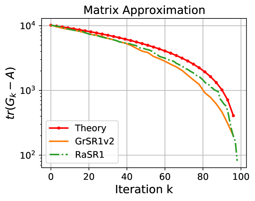
(a) $d=100,\varkappa=2000$.

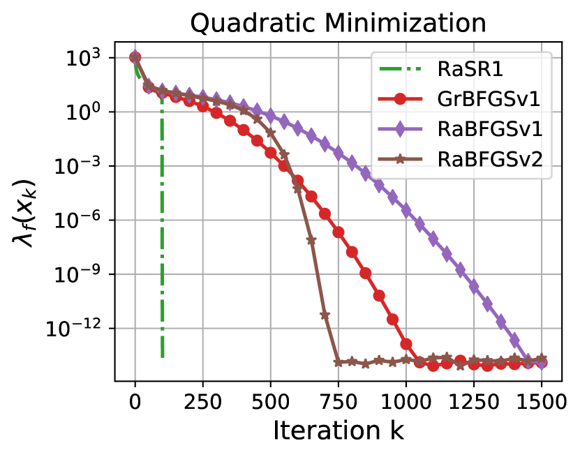
(b) $d=100,\varkappa=2000$.

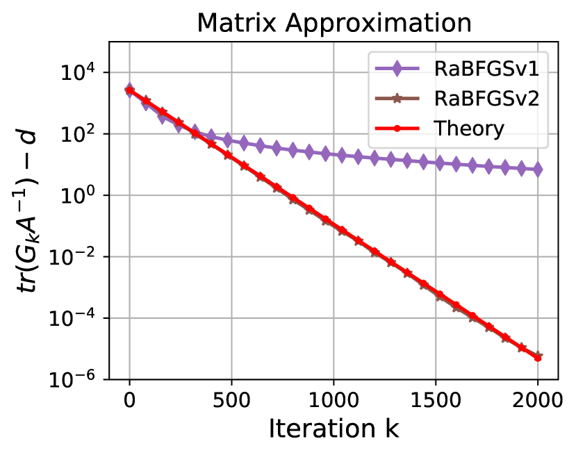
(c) $d=100,\varkappa=200$.

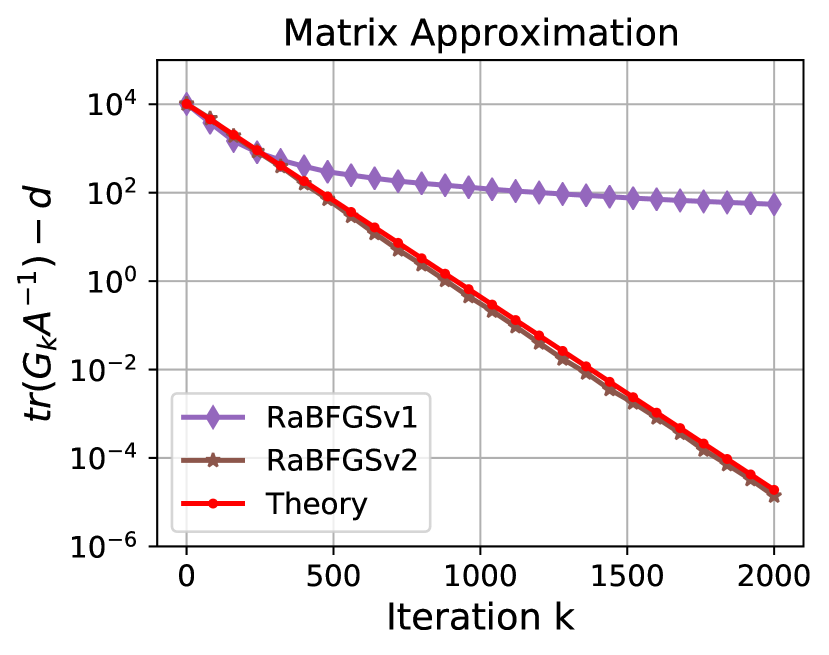
(d) $d=100,\varkappa=2000$.

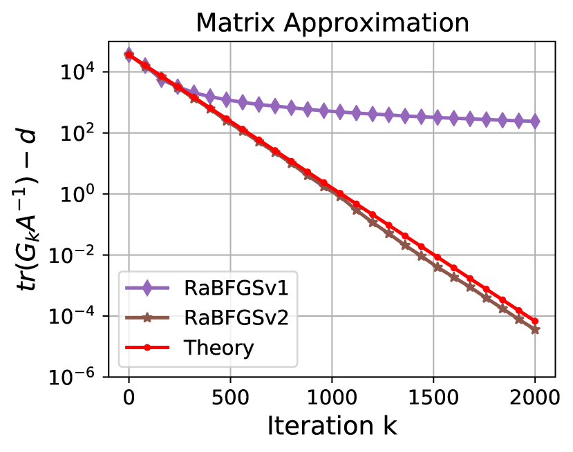
(e) $d=100,\varkappa=20000$.

Figure 1: (a, c, d, e) Comparison of different direction choosing methods under the SR1 or BFGS update for approximating a matrix ${\bm{A}}$ that $\mu{\bm{I}}_{d}\preceq{\bm{A}}\preceq L{\bm{I}}_{d}$ from ${\bm{G}}_{0}=L{\bm{I}}_{d}$. (a) The variation of $\tau_{\bm{A}}({\bm{G}}_{k})$ during Random SR1 (RaSR1) and our Greedy SR1 (GrSR1v2) update with nearly matched upper bound. (c,d,e) The variation of $\sigma_{\bm{A}}({\bm{G}}_{k})$ during our Random BFGS (RaBFGSv2) update and the original random version (RaBFGSv1) under various condition numbers. (b) Comparison of SR1 and BFGS methods for quadratic objective. Here we only depict RaSR1 method, while the other SR1-type methods share similar behavior.

Matrix approximation.

When using Algorithms 4 and 5 for approximating a matrix ${\bm{A}}\succ 0$, we show the measure as proved by Theorems 13 and 14 in Figures 1(a), 1(c),1(d) and 1(e). As Figure 1(a) depicts, our greedy and random SR1 updates (GrSR1v2 and RaSR1) share superlinear convergence rates under measure $\tau_{\bm{A}}(\cdot)$, while our theoretical bound matches them well. Moreover, Figures 1(c), 1(d) and 1(e) describe the behavior of the random BFGS update under different condition numbers. Our theory matches the linear convergence of measure $\sigma_{\bm{A}}(\cdot)$ in our modified random BFGS update (RaBFGSv2) across different $\varkappa$s. While directly choosing a direction without scaling (RaBFGSv1) fails to give such bounds. Particularly, a large condition number could cause slow convergence of RaBFGSv1. Hence, our methods provide effective ways of approaching a positive definite Hessian matrix.

Quadratic minimization.

We also consider unconstrained quadratic minimization in Eq. (14) with the same positive definite matrix ${\bm{A}}$ and a randomly selected vector ${\bm{b}}\in{\mathbb{R}}^{d}$. Running Algorithm 6 with SR1 and BFGS updates, we obtain the superlinear convergence of $\lambda_{f}(\cdot)$ shown in Figure 1(b). Not surprisingly, our RaBFGSv2 runs faster than RaBFGSv1, while we also have the theoretical guarantee. At the same time, SR1-type methods converge to zero after $d+1$ steps because of ${\bm{G}}_{d}={\bm{A}}$ almost surely. Here, we only depict the RaSR1 update, while the other SR1-type methods share similar behavior. Although our theoretical bound can not directly match the experiments due to the related initial terms $\tau_{\bm{A}}({\bm{G}}_{0})$ and $\sigma_{\bm{A}}({\bm{G}}_{0})$, the decay terms: $\left(1-k/d\right)$ vs. $\left(1-1/d\right)^{k}$ already show the superiority of the SR1 method over the BFGS method in the quadratic minimization problem.

Regularized Log-Sum-Exp.

Following the work of Rodomanov and Nesterov (2021b), we present computational results for greedy and random quasi-Newton methods, applied to the following test function with ${\bm{C}}=\left[{\bm{c}}_{1},\ldots,{\bm{c}}_{m}\right]\in{\mathbb{R}}^{d\times m}$, $b_{1},\dots,b_{m}\in{\mathbb{R}}$, and $\gamma>0$:

$$f({\bm{x}}):=\ln\left(\sum_{j=1}^{m}e^{{\bm{c}}_{j}^{\top}{\bm{x}}-b_{j}}\right)+\frac{1}{2}\sum_{j=1}^{m}\left({\bm{c}}_{j}^{\top}{\bm{x}}\right)^{2}+\frac{\gamma}{2}\left\|{\bm{x}}\right\|^{2},{\bm{x}}\in{\mathbb{R}}^{d}.$$

We need access to the gradient of function $f({\bm{x}})$:

$$\nabla f({\bm{x}})=g({\bm{x}})+\sum_{j=1}^{m}\left({\bm{c}}_{j}^{\top}{\bm{x}}\right){\bm{c}}_{j}+\gamma{\bm{x}},\text{ with }g({\bm{x}}):=\sum_{j=1}^{m}\pi_{j}({\bm{x}}){\bm{c}}_{j},$$

where

$$\pi_{j}({\bm{x}}):=\frac{e^{{\bm{c}}_{j}^{\top}{\bm{x}}-b_{j}}}{\sum_{i=1}^{m}e^{{\bm{c}}_{i}^{\top}{\bm{x}}-b_{i}}}\in[0,1],j=1,\dots,m.$$

Moreover, given a point ${\bm{x}}\in{\mathbb{R}}^{d}$, we need to be able to perform the following two actions:

$${\bm{e}}_{i}^{\top}[\nabla^{2}f({\bm{x}})]{\bm{e}}_{i}=\sum_{j=1}^{m}\left(\pi_{j}({\bm{x}})+1\right)({\bm{c}}_{j}^{\top}{\bm{e}}_{i})^{2}-(g({\bm{x}})^{\top}{\bm{e}}_{i})^{2}+\gamma,\forall 1\leq i\leq d,$$

and for a given direction ${\bm{h}}\in{\mathbb{R}}^{d}$,

$$\nabla^{2}f({\bm{x}})\cdot{\bm{h}}=\sum_{j=1}^{m}\left(\pi_{j}({\bm{x}})+1\right)\left({\bm{c}}_{j}^{\top}{\bm{h}}\right){\bm{c}}_{j}-\left(g({\bm{x}})^{\top}{\bm{h}}\right)g({\bm{x}})+\gamma{\bm{h}}.$$

Thus both the above operations have a cost of $O(md)$. Thus, the cost of one iteration for all the methods is comparable. Furthermore, note that

$$\nabla^{2}f({\bm{x}})=\sum_{j=1}^{m}\left(\pi_{j}({\bm{x}})+1\right){\bm{c}}_{j}{\bm{c}}_{j}^{\top}-g({\bm{x}})g({\bm{x}})^{\top}+\gamma{\bm{I}}_{d}.$$

We get the Lipschitz constant of $\nabla f({\bm{x}})$ can be taken as $L=2\lambda_{\max}({\bm{C}}{\bm{C}}^{\top})+\gamma$, and $\varkappa=L/\gamma$. As mentioned in the work of Rodomanov and Nesterov (2021b, Section 5.1), the strong self-concordancy parameter is $M=2$ with respect to the operator $\sum_{j=1}^{m}{\bm{c}}_{j}{\bm{c}}_{j}^{\top}$.

We also adopt the same synthetic data as used by Rodomanov and Nesterov (2021b, Section 5.1). First, we generate a collection of random vectors $\hat{{\bm{c}}}_{1},\ldots,\hat{{\bm{c}}}_{m}$ with entries, uniformly distributed in the interval $[-1,1]$. Then we generate $b_{1},\dots,b_{m}$ from the same distribution. Using this data, we define

$$\forall 1\leq j\leq m,\;{\bm{c}}_{j}:=\hat{{\bm{c}}}_{j}-\nabla\hat{f}(\bm{0}),\text{ where }\hat{f}({\bm{x}}):=\ln\bigg{(}\sum_{j=1}^{m}e^{\hat{{\bm{c}}}_{j}^{\top}{\bm{x}}-b_{j}}\bigg{)}.$$

Note that by construction,

$$\nabla f(\bm{0})=\frac{1}{\sum_{i=1}^{m}e^{-b_{i}}}\sum_{j=1}^{m}e^{-b_{j}}\left(\hat{{\bm{c}}}_{j}-\nabla\hat{f}(\bm{0})\right)=\bm{0}.$$

So the unique minimizer of our test function is ${\bm{x}}_{*}=\bm{0}$. The starting point ${\bm{x}}_{0}$ for all methods is the same and generated randomly from the uniform distribution on the standard Euclidean sphere of radius $1/d$ centered at the minimizer, i.e., ${\bm{x}}_{0}\sim\text{Unif}\left(\frac{1}{d}{\mathcal{S}}^{d-1}\right)$. We compare $\left\|\nabla f({\bm{x}}_{k})\right\|$ obtained by different methods.

As Figure 2 depicts, the BFGS-type methods are slower than the SR1-type methods, and the greedy algorithms converge more rapidly than the random algorithms. The only difference is that our RaBFGSv2 may have slower convergence behavior than RaBFGSv1 under a small $\varkappa$ in Figure 2(a).

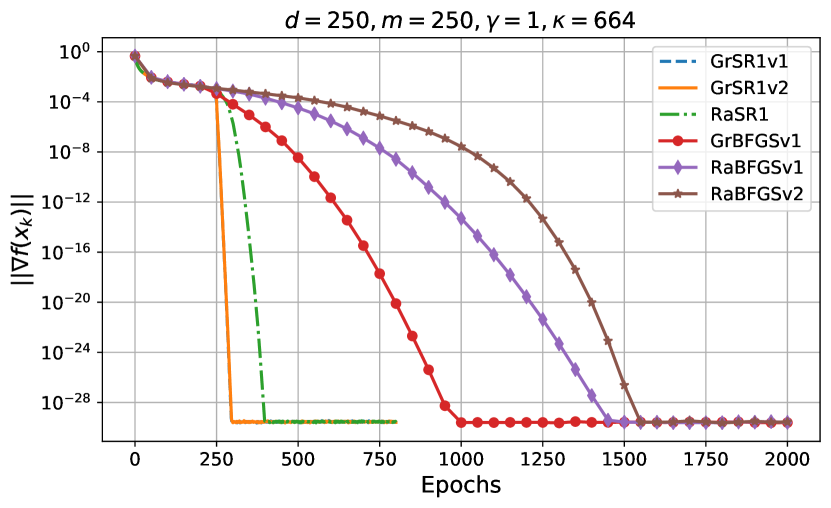
(a) $\gamma=1,\varkappa=664$.

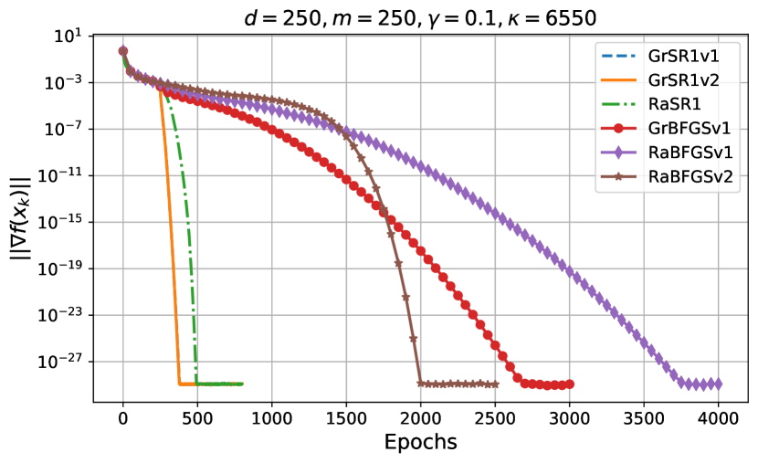
(b) $\gamma=0.1,\varkappa=6550$.

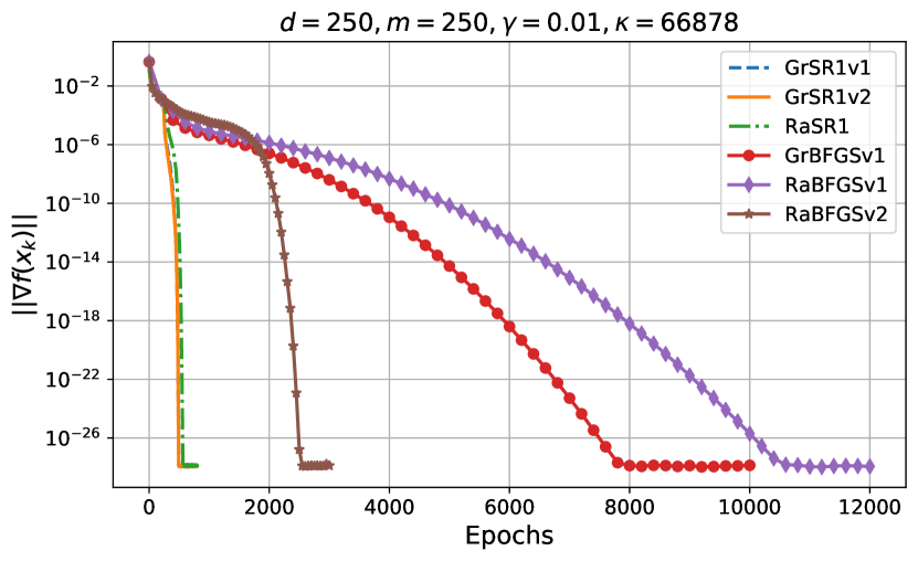
(c) $\gamma=0.01,\varkappa=66878$.

Figure 2: Comparison of SR1 and BFGS updates for Regularized Log-Sum-Exp. The dimension $d$, the number $m$ of linear functions, the regularization coefficient $\gamma$ and condition number $\varkappa$ are displayed in the title of each graph. The lines of GrSR1v1 and GrSR1v2 are overlapped in each figure.

We consider our scaled direction is more suitable for a constant Hessian matrix as the quadratic objective has. Thus we still have a better convergence rate in the last few iterations when Hessians are nearly unchanged in Figure 2(a). However, the Hessian varies drastically in the initial period. Thus there is less benefit under a more accurate Hessian approximation. When applied to the ill-conditioning setting with a large $\varkappa$ in Figures 2(b) and 2(c), we find our RaBFGSv2 could be faster than GrBFGSv1 and RaBFGSv1. This implies that our proposed method has less dependence on the condition number $\varkappa$.

Regularized Logistic Regression.

Finally, we consider a common machine learning problem: $\ell_{2}$-regularized logistic regression, which has the objective as

$$f({\bm{w}})=\sum_{i=1}^{n}\ln\left(1+e^{-y_{i}{\bm{w}}^{\top}{\bm{x}}_{i}}\right)+\frac{\gamma}{2}\|{\bm{w}}\|^{2},\;{\bm{w}}\in{\mathbb{R}}^{d},$$

where ${\bm{X}}=\left[{\bm{x}}_{1},\dots,{\bm{x}}_{n}\right]\in{\mathbb{R}}^{d\times n}$ are training samples, the corresponding labels are $y_{1},\dots,y_{n}$
$\in\{+1,-1\}$, and $\gamma>0$ is the regularization coefficient. The gradient of function $f({\bm{w}})$ is

$$\nabla f({\bm{w}})=-\sum_{i=1}^{n}\frac{1}{1+e^{y_{i}{\bm{w}}^{\top}{\bm{x}}_{i}}}\cdot y_{i}{\bm{x}}_{i}+\gamma{\bm{w}},\;{\bm{w}}\in{\mathbb{R}}^{d}.$$

Moreover, given a point ${\bm{w}}\in{\mathbb{R}}^{d}$, we need to be able to perform the following two actions:

$${\bm{e}}_{j}^{\top}[\nabla^{2}f({\bm{w}})]{\bm{e}}_{j}=\sum_{i=1}^{n}\frac{e^{y_{i}{\bm{w}}^{\top}{\bm{x}}_{i}}}{\left(1+e^{y_{i}{\bm{w}}^{\top}{\bm{x}}_{i}}\right)^{2}}\cdot({\bm{x}}_{i}^{\top}{\bm{e}}_{j})^{2}+\gamma,\forall 1\leq j\leq d,$$

and for a given ${\bm{h}}\in{\mathbb{R}}^{d}$,

$$\nabla^{2}f({\bm{w}})\cdot{\bm{h}}=\sum_{i=1}^{n}\frac{e^{y_{i}{\bm{w}}^{\top}{\bm{x}}_{i}}}{\left(1+e^{y_{i}{\bm{w}}^{\top}{\bm{x}}_{i}}\right)^{2}}\cdot\left({\bm{x}}_{i}^{\top}{\bm{h}}\right)\cdot{\bm{x}}_{i}+\gamma{\bm{h}}.$$

Thus, both the above operations have a cost of $O(nd)$. Furthermore, note that

$$\nabla^{2}f({\bm{w}})=\sum_{i=1}^{n}\frac{e^{y_{i}{\bm{w}}^{\top}{\bm{x}}_{i}}}{\left(1+e^{y_{i}{\bm{w}}^{\top}{\bm{x}}_{i}}\right)^{2}}\cdot{\bm{x}}_{i}{\bm{x}}_{i}^{\top}+\gamma{\bm{I}}_{d},\;{\bm{w}}\in{\mathbb{R}}^{d}.$$

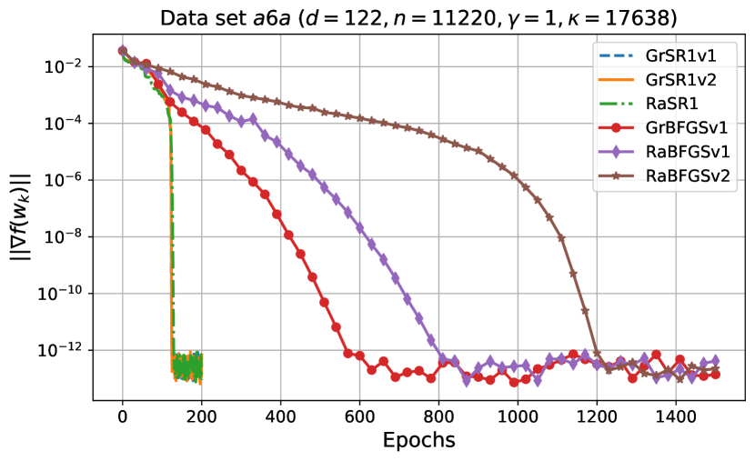
(a) $\gamma=1,\varkappa=17638$.

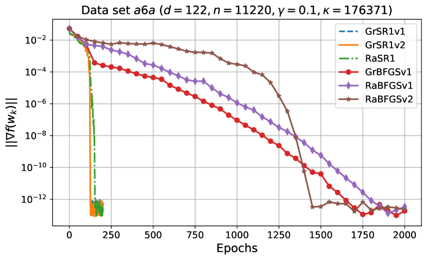
(b) $\gamma=0.1,\varkappa=176371$.

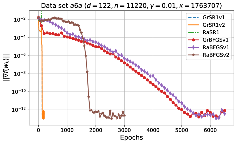
(c) $\gamma=0.01,\varkappa=1763707$.

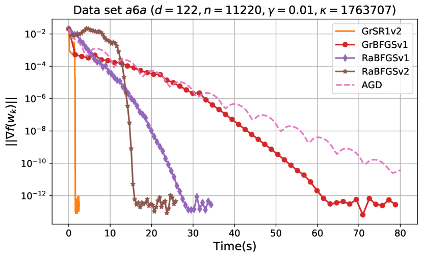
(d) $\gamma=0.01,\varkappa=1763707$.

Figure 3: Comparison of SR1 and BFGS update for $\ell_{2}$-regularized logistic regression applied with ‘a6a’ data from the LIBSVM collection of real-world datasets. We list the name of dataset, the dimension $d$ and the condition number $\varkappa$ under the corresponding $\gamma$ in the title of each figure. (a,b,c) Comparison of convergence rates with various condition numbers. The lines of GrSR1v1 and GrSR1v2 are overlapped in some figures, and RaSR1 fails when $\gamma=0.01$ due to the unsuitable initialization and search directions. (d) Comparison of running time with AGD when $\gamma=0.01$.

We obtain that the Lipschitz constant of $\nabla f({\bm{w}})$ can be taken as $L=\frac{\lambda_{\max}({\bm{X}}{\bm{X}}^{\top})}{4}+\gamma$, and $\varkappa=L/\gamma$. Additionally, we take data from the LIBSVM collection of real-world datasets for binary classification problems (Chang and Lin, 2011). And we do not apply the correction strategy (i.e., $\tilde{{\bm{G}}}_{k}=(1+Mr_{k}){\bm{G}}_{k}$) shown in Algorithm 7 recommended by Rodomanov and Nesterov (2021b, Section 5.2). In order to simulate the local convergence, we use the same initialization after running several standard Newton’s steps to make the measure $\left\|\nabla f({\bm{w}}_{0})\right\|$ small (around $10^{-2}\sim 10^{0}$). We compare $\left\|\nabla f({\bm{w}}_{k})\right\|$ obtained by different methods.

We show the results in Figure 3. As we can see, the general picture is the same as the Regularized Log-Sum-Exp. In particular, SR1-type methods are still faster than BFGS-type methods, and the greedy algorithms also converge more rapidly than the random algorithms. GrBFGSv1 and RaBFGSv1 are faster than RaBFGSv2 in a small condition number case in Figure 3(a), but they become slower than RaBFGSv2 when the condition number becomes huge in Figures 3(b) and 3(c). Therefore, we think our RaBFGSv2 which uses scaled direction indeed has less dependence on the condition number as our theory shows.

In addition, we also compare the running time of each method with a classical first-order method: accelerated gradient descent (AGD) following Nesterov (2003). We run the standard AGD algorithm for $25000$ epochs with the same setting in Figure 3(c). As Figure 3(d) shows, not surprisingly, we could discover the benefit of quasi-Newton methods in running time due to their superlinear convergence rates. Furthermore, we find that GrBFGSv1 takes more time compared to the other methods because of the greedy step for searching directions. Thus, the greedy method is time-consuming as Rodomanov and Nesterov (2021b) discussed. But the random method solves this problem through a random choice of directions. Moreover, we discover that random methods may fail for unsuitable initialization as the RaSR1 method in Figure 3(c) shows, since we may encounter bad random directions during iterations, and our theoretical guarantee is also a probabilistic description. Hence, we recommend a mixture of greedy and random strategies in practice to balance the convergence and running complexity.

Overall, our proposed methods do not lose the superlinear convergence rates particularly in the large condition number schemes, while we also present the theoretical guarantee for these algorithms.

7 Conclusion

In this work, we have addressed two open problems mentioned by Rodomanov and Nesterov (2021b). First, we have shown theoretical analysis of the random quasi-Newton methods, which also preserve a similar nonasymptotic superlinear convergence shown in the work of Rodomanov and Nesterov (2021b). Second, we have studied the behavior of two specific famous quasi-Newton methods: the SR1 and BFGS methods. We have presented different greedy methods in contrast to the work of Rodomanov and Nesterov (2021b), as well as the random version of these methods. In particular, we have provided the faster Hessian approximation behavior and the condition-number-free (local) superlinear convergence rates applied to quadratic or strongly self-concordant objectives. Moreover, the experiments match our analysis well. We hope that the theoretical analysis and the related work would be useful for understanding the explicit rates of quasi-Newton methods, and such convergence rates could benefit machine learning by developing new optimization methods.

Acknowledgments

We would like to thank the anonymous reviewers for their careful work and constructive comments that greatly help us improve the paper quality. We also thank an anonymous reviewer for pointing out efficient update in Proposition 16 and concise formulation in Lemmas 10 and 18, as well as providing a special lemma (Lemma 25) in Appendix.

Haishan Ye has been supported by the National Natural Science Foundation of China (No. 12101491).

Appendix A Auxiliary Lemmas and Theorems

In the following, assume the objective $f({\bm{x}})$ is an $M$-strongly self-concordant, $\mu$-strongly convex and $L$-smooth function as Subsection 3.3 does.

Lemma 21

(Rodomanov and Nesterov, 2021b, Lemma 4.2) Let ${\bm{x}},\bm{y}\in{\mathbb{R}}^{d}$, and $r:=\|\bm{y}-{\bm{x}}\|_{{\bm{x}}}$. Then we have

$$\frac{\nabla^{2}f({\bm{x}})}{1+Mr}\preceq\nabla^{2}f(\bm{y})\preceq\left(1+Mr\right)\nabla^{2}f({\bm{x}}).$$ (29)

Also, for ${\bm{J}}:=\int_{0}^{1}\nabla^{2}f({\bm{x}}+t(\bm{y}-{\bm{x}}))dt$ and any $\bm{v}\in\{{\bm{x}},\bm{y}\}$, we have

$$\frac{\nabla^{2}f(\bm{v})}{1+\frac{Mr}{2}}\preceq{\bm{J}}\preceq\left(1+\frac{Mr}{2}\right)\nabla^{2}f(\bm{v}).$$

Lemma 22

(Rodomanov and Nesterov, 2021b, Lemmas 4.3 and 4,4) Let ${\bm{x}}\in{\mathbb{R}}^{d}$, and a symmetric matrix ${\bm{G}}$, such that $\nabla^{2}f({\bm{x}})\preceq{\bm{G}}\preceq\eta\nabla^{2}f({\bm{x}})$, for some $\eta\geq 1$. Let ${\bm{x}}_{+}\in{\mathbb{R}}^{d}$, and $r=\|{\bm{x}}_{+}-{\bm{x}}\|_{{\bm{x}}}$. Then we have

$$\tilde{{\bm{G}}}:=\left(1+Mr\right){\bm{G}}\succeq\nabla^{2}f({\bm{x}}_{+}),$$ (30)

and for all $\bm{u}\in{\mathbb{R}}^{d}$ and $\tau\in[0,1]$, we have

$$\nabla^{2}f({\bm{x}}_{+})\preceq\mathrm{Broyd}_{\tau}\left(\tilde{{\bm{G}}},\nabla^{2}f({\bm{x}}_{+}),\bm{u}\right)\preceq\left[\left(1+Mr\right)^{2}\eta\right]\nabla^{2}f({\bm{x}}_{+}).$$ (31)

More specifically, if ${\bm{x}}_{+}={\bm{x}}-{\bm{G}}^{-1}\nabla f({\bm{x}})$, and letting $\lambda:=\lambda_{f}({\bm{x}})$ be such that $M\lambda\leq 2$, then,

$$r\leq\lambda,\text{ and }\lambda_{f}({\bm{x}}_{+})\leq\left(1+\frac{M\lambda}{2}\right)\frac{\eta-1+\frac{M\lambda}{2}}{\eta}\cdot\lambda.$$ (32)

Theorem 23

(Extension of Rodomanov and Nesterov, 2021b, Theorem 4.7) Suppose in Algorithm 8, a (random) initialization ${\bm{G}}_{0}$ satisfies

$$\nabla^{2}f({\bm{x}}_{0})\preceq{\bm{G}}_{0}\preceq\eta\nabla^{2}f({\bm{x}}_{0})$$ (33)

for some $\eta\geq 1$, and the (random) initial point ${\bm{x}}_{0}$ is sufficiently close to the solution:

$$M\lambda_{0}\leq\frac{\ln\frac{3}{2}}{4\eta}.$$ (34)

Then, for all $k\geq 0$, we have

$$\nabla^{2}f({\bm{x}}_{k})\preceq{\bm{G}}_{k}\preceq e^{2M\sum_{i=0}^{k-1}\lambda_{i}}\eta\nabla^{2}f({\bm{x}}_{k})\preceq\frac{3\eta}{2}\nabla^{2}f({\bm{x}}_{k}),$$ (35)

and

$$\lambda_{k}\leq\left(1-\frac{1}{2\eta}\right)^{k}\lambda_{0},$$ (36)

where $\lambda_{k}$ is defined in Eqs. (3) and (4).

Algorithm 8 Quasi-Newton Method (Rodomanov and Nesterov, 2021b, Scheme (4.17))

1:  Initialization: Choose ${\bm{G}}_{0}\succeq\nabla^{2}f({\bm{x}}_{0})$ (such as ${\bm{G}}_{0}=L{\bm{I}}_{d}$).

2:  for $k\geq 0$ do

3:     Update ${\bm{x}}_{k+1}={\bm{x}}_{k}-{\bm{G}}_{k}^{-1}\nabla f({\bm{x}}_{k})$.

4:     Compute $r_{k}=\|{\bm{x}}_{k+1}-{\bm{x}}_{k}\|_{{\bm{x}}_{k}}$ and set $\tilde{{\bm{G}}}_{k}=\left(1+Mr_{k}\right){\bm{G}}_{k}$.

5:     Choose $\bm{u}_{k}\in{\mathbb{R}}^{d}$ and $\tau_{k}\in[0,1]$.

6:     Compute ${\bm{G}}_{k+1}=\mathrm{Broyd}_{\tau_{k}}\left(\tilde{{\bm{G}}}_{k},\nabla^{2}f({\bm{x}}_{k+1}),\bm{u}_{k}\right)$.

7:  end for

Proof  The proof is similar as Theorem 4.7 by Rodomanov and Nesterov (2021b). We give the detail for completeness.

From Eq. (33), both Eqs. (35) and (36) are satisfied for $k=0$. Now let $k\geq 0$, and suppose Eqs. (35) and (36) have already been proved for all $0\leq k^{\prime}\leq k$. Denote

$$\eta_{k}:=e^{2M\sum_{i=0}^{k-1}\lambda_{i}}\eta.$$ (37)

Then by inductive hypothesis, we have

$$\nabla^{2}f({\bm{x}}_{k})\preceq{\bm{G}}_{k}\preceq\eta_{k}\nabla^{2}f({\bm{x}}_{k}).$$ (38)

Note that

$$M\sum_{i=0}^{k}\lambda_{i}\stackrel{{\scriptstyle\eqref{eq:lambda-a}}}{{\leq}}M\lambda_{0}\sum_{i=0}^{k}\left(1-\frac{1}{2\eta}\right)^{i}\leq 2\eta M\lambda_{0}\stackrel{{\scriptstyle\eqref{eq:init-linear}}}{{\leq}}\frac{\ln\frac{3}{2}}{2}<1.$$ (39)

Hence, $M\lambda_{k}<2$, and by Lemma 22, we have

$$r_{k}:=\|{\bm{x}}_{k+1}-{\bm{x}}_{k}\|_{{\bm{x}}_{k}}\stackrel{{\scriptstyle\eqref{eq:lam-eta}}}{{\leq}}\lambda_{k},$$ (40)

and

$$\lambda_{k+1}\stackrel{{\scriptstyle\eqref{eq:lam-eta}\eqref{eq:hess}}}{{\leq}}\left(1+\frac{M\lambda_{k}}{2}\right)\frac{\eta_{k}-1+\frac{M\lambda_{k}}{2}}{\eta_{k}}\lambda_{k}\leq\left(1+\frac{M\lambda_{k}}{2}\right)\left(1-\frac{1-\frac{M\lambda_{k}}{2}}{\eta_{k}}\right)\lambda_{k}.$$ (41)

Using the inequality $1-t\geq e^{-2t}$ when $0\leq t\leq 1/2$, we get

$$\frac{1-\frac{M\lambda_{k}}{2}}{\eta_{k}}\stackrel{{\scriptstyle\eqref{eq:m-lam-ran-1}}}{{\geq}}e^{-M\lambda_{k}}\eta_{k}^{-1}\stackrel{{\scriptstyle\eqref{eq:etak}}}{{\geq}}e^{-2M\sum_{i=0}^{k}\lambda_{i}}\eta^{-1}\stackrel{{\scriptstyle\eqref{eq:m-lam-ran-1}}}{{\geq}}\frac{2}{3\eta}.$$

Moreover, noting that $M\lambda_{k}\stackrel{{\scriptstyle\eqref{eq:lambda-a}}}{{\leq}}M\lambda_{0}\stackrel{{\scriptstyle\eqref{eq:init-linear}}}{{\leq}}\frac{1}{8\eta}$, we obtain

$$\left(1+\frac{M\lambda_{k}}{2}\right)\left(1-\frac{1-\frac{M\lambda_{k}}{2}}{\eta_{k}}\right)\leq\left(1+\frac{1}{16\eta}\right)\left(1-\frac{2}{3\eta}\right)\leq 1-\frac{2}{3\eta}+\frac{1}{16\eta}\leq 1-\frac{1}{2\eta}.$$

Consequently,

$$\lambda_{k+1}\stackrel{{\scriptstyle\eqref{eq:lam-re-ran-1}}}{{\leq}}\left(1-\frac{1}{2\eta}\right)\lambda_{k}\stackrel{{\scriptstyle\eqref{eq:lambda-a}}}{{\leq}}\left(1-\frac{1}{2\eta}\right)^{k+1}\lambda_{0}.$$

Finally, from Eq. (31) in Lemma 22, it follows that

$$\nabla^{2}f({\bm{x}}_{k+1}) \preceq {\bm{G}}_{k+1}\preceq\left(1+Mr_{k}\right)^{2}\eta_{k}\nabla^{2}f({\bm{x}}_{k+1})\stackrel{{\scriptstyle\eqref{eq:r-lam-ran-1}}}{{\preceq}}\left(1+M\lambda_{k}\right)^{2}\eta_{k}\nabla^{2}f({\bm{x}}_{k+1})$$

$$\preceq e^{2M\lambda_{k}}\eta_{k}\nabla^{2}f({\bm{x}}_{k+1})\stackrel{{\scriptstyle\eqref{eq:etak}}}{{=}}e^{2M\sum_{i=0}^{k}\lambda_{i}}\eta\nabla^{2}f({\bm{x}}_{k+1})\stackrel{{\scriptstyle\eqref{eq:m-lam-ran-1}}}{{\preceq}}\frac{3\eta}{2}\nabla^{2}f({\bm{x}}_{k+1}).$$

Thus, Eqs. (35) and (36) are valid for index $k+1$, and we can continue by induction.  

Remark 24

Note that the choice of $\{{\bm{u}}_{k}\}$ and the update rule in Algorithm 8 are arbitrary, thus Algorithms 3 and 7 can be viewed as special cases of Algorithm 8. Therefore, Theorem 23 always holds as long as the initial point ${\bm{x}}_{0}$ is always sufficiently close to the solution based on the initial approximate matrix ${\bm{G}}_{0}$, and Eq. (36) holds without any expectations.

Lemma 25

(Extension of Rodomanov and Nesterov, 2021b, Lemma 4.8)  
Following the update in Algorithms 3 or 7, we can obtain

$$\forall k\geq 0,\nabla^{2}f({\bm{x}}_{k})\preceq{\bm{G}}_{k}\preceq(1+\delta_{k})\nabla^{2}f({\bm{x}}_{k}),$$ (42)

where $\delta_{k}$ is a random sequence which satisfies the following recurrence:

$$\mathbb{E}_{{\bm{u}}_{k}}\delta_{k+1}\leq\left(1-t^{-1}\right)\left(1+Mr_{k}\right)^{2}\left(\delta_{k}+2cdMr_{k}\right)$$ (43)

for some constants $c,t\geq 1$. Particularly,

1. for the Broyden method in Algorithm 3, one has $\delta_{k}=\sigma_{k},t=d\varkappa,c=1$;

2. for the BFGS method in Algorithm 7, one has $\delta_{k}=\sigma_{k},t=d,c=1$;

3. for the SR1 method in Algorithm 7, one has $\delta_{k}=d\varkappa\tau_{k}/\mathrm{tr}[\nabla^{2}f({\bm{x}}_{k})],t=d,c=\varkappa$.

Here, $r_{k}:=\|{\bm{x}}_{k+1}-{\bm{x}}_{k}\|_{{\bm{x}}_{k}},\sigma_{k}$ and $\tau_{k}$ are defined in Eq. (4).

Proof  From the update rule in Algorithms 3 and 7, we apply Lemma 22 to obtain

$${\bm{G}}_{k}\stackrel{{\scriptstyle\eqref{eq:tg}}}{{\succeq}}\nabla^{2}f({\bm{x}}_{k}),\;\forall k\geq 0.$$ (44)

Now for all $k\geq 0$, we define $\eta_{k}=\left\|[\nabla^{2}f({\bm{x}}_{k})]^{-1/2}{\bm{G}}_{k}[\nabla^{2}f({\bm{x}}_{k})]^{-1/2}\right\|$. Then $\eta_{k}\stackrel{{\scriptstyle\eqref{eq:g-hes}}}{{\geq}}1$ and ${\bm{G}}_{k}\preceq\eta_{k}\nabla^{2}f({\bm{x}}_{k})$. Hence,

$$\eta_{k}-1 =\left\|[\nabla^{2}f({\bm{x}}_{k})]^{-1/2}({\bm{G}}_{k}-\nabla^{2}f({\bm{x}}_{k}))[\nabla^{2}f({\bm{x}}_{k})]^{-1/2}\right\|$$

$$\leq\mathrm{tr}\left([\nabla^{2}f({\bm{x}}_{k})]^{-1/2}\left({\bm{G}}_{k}-\nabla^{2}f({\bm{x}}_{k})\right)[\nabla^{2}f({\bm{x}}_{k})]^{-1/2}\right)\stackrel{{\scriptstyle\eqref{eq:lam-sig}}}{{=}}\sigma_{k}.$$

Moreover, from $\mu{\bm{I}}_{d}\preceq\nabla^{2}f({\bm{x}}_{k})\preceq L{\bm{I}}_{d},\forall k\geq 0$, we also have

$$\eta_{k}-1 =\left\|[\nabla^{2}f({\bm{x}}_{k})]^{-1/2}({\bm{G}}_{k}-\nabla^{2}f({\bm{x}}_{k}))[\nabla^{2}f({\bm{x}}_{k})]^{-1/2}\right\|\leq\frac{\|{\bm{G}}_{k}-\nabla^{2}f({\bm{x}}_{k})\|}{\mu}$$

$$\leq\frac{\mathrm{tr}\left[{\bm{G}}_{k}-\nabla^{2}f({\bm{x}}_{k})\right]}{\mu}\stackrel{{\scriptstyle\eqref{eq:lam-sig}}}{{=}}\frac{\tau_{k}}{\mu}\leq\frac{dL}{\mathrm{tr}[\nabla^{2}f({\bm{x}}_{k})]}\cdot\frac{\tau_{k}}{\mu}=\frac{d\varkappa\tau_{k}}{\mathrm{tr}[\nabla^{2}f({\bm{x}}_{k})]}.$$

Therefore, the choices of $\delta_{k}=\sigma_{k}$ and $\frac{d\varkappa\tau_{k}}{\mathrm{tr}[\nabla^{2}f({\bm{x}}_{k})]}$ are valid to guarantee Eq. (42). Next, we deduce Eq. (43) based on the specific choice of $\delta_{k}$.

1) For the Broyden method in Algorithm 3, by Theorem 6, one step update gives

$$\mathbb{E}_{{\bm{u}}_{k}}\sigma_{k+1}\stackrel{{\scriptstyle\eqref{eq:lam-sig}}}{{=}}\mathbb{E}_{{\bm{u}}_{k}}\sigma_{\nabla^{2}f({\bm{x}}_{k+1})}\left({\bm{G}}_{k+1}\right)\stackrel{{\scriptstyle\eqref{eq:random-k}}}{{\leq}}\left(1-\frac{1}{d\varkappa}\right)\sigma_{\nabla^{2}f({\bm{x}}_{k+1})}(\tilde{{\bm{G}}}_{k}),\forall k\geq 0.$$

We deduce the result by bounding the last term as below:

$$\sigma_{\nabla^{2}f({\bm{x}}_{k+1})}(\tilde{\bm{G}}_{k}) \stackrel{{\scriptstyle\eqref{eq:sigmaA}}}{{=}} \mathrm{tr}\left([\nabla^{2}f({\bm{x}}_{k+1})]^{-1}\tilde{{\bm{G}}}_{k}\right){-}d=\left(1{+}Mr_{k}\right)\mathrm{tr}\left([\nabla^{2}f({\bm{x}}_{k+1})]^{-1}{\bm{G}}_{k}\right){-}d$$ (45)

$$\stackrel{{\scriptstyle\eqref{eq:fr}}}{{\leq}} \left(1{+}Mr_{k}\right)^{2}\mathrm{tr}\left([\nabla^{2}f({\bm{x}}_{k})]^{-1}{\bm{G}}_{k}\right){-}d\stackrel{{\scriptstyle\eqref{eq:lam-sig}}}{{=}}\left(1{+}Mr_{k}\right)^{2}\left(\sigma_{k}{+}d\right){-}d$$

$$= \left(1{+}Mr_{k}\right)^{2}\sigma_{k}{+}d\left[2Mr_{k}{+}(Mr_{k})^{2}\right]\leq\left(1{+}Mr_{k}\right)^{2}\left(\sigma_{k}{+}2dMr_{k}\right).$$

2) For the BFGS method in Algorithm 7, by Theorem 14, one step update gives

$$\mathbb{E}_{{\bm{u}}_{k}}\sigma_{k+1}\stackrel{{\scriptstyle\eqref{eq:sigma-k}}}{{\leq}}\left(1-\frac{1}{d}\right)\sigma_{\nabla^{2}f({\bm{x}}_{k+1})}(\tilde{{\bm{G}}}_{k}),\forall k\geq 0.$$

The remaining proof is the same as Eq. (45).

3) For the SR1 method in Algorithm 7, from Theorem 13, one step update gives

$$\mathbb{E}_{{\bm{u}}_{k}}\tau_{k+1}\stackrel{{\scriptstyle\eqref{eq:tau-k}}}{{\leq}}\left(1-\frac{1}{d}\right)\tau_{\nabla^{2}f({\bm{x}}_{k+1})}(\tilde{{\bm{G}}}_{k}),\forall k\geq 0.$$

Now we can bound the last term as below:

$$\tau_{\nabla^{2}f({\bm{x}}_{k+1})}(\tilde{{\bm{G}}}_{k}) \stackrel{{\scriptstyle\eqref{eq:lam-sig}}}{{=}} \mathrm{tr}\left(\tilde{{\bm{G}}}_{k}-\nabla^{2}f({\bm{x}}_{k+1})\right)\stackrel{{\scriptstyle\eqref{eq:fr}}}{{\leq}}\mathrm{tr}\left(\left(1+Mr_{k}\right){\bm{G}}_{k}-\frac{\nabla^{2}f({\bm{x}}_{k})}{1+Mr_{k}}\right)$$

$$\stackrel{{\scriptstyle\eqref{eq:lam-sig}}}{{=}} \left(1+Mr_{k}\right)\tau_{k}+\left(1+Mr_{k}-\frac{1}{1+Mr_{k}}\right)\mathrm{tr}\left[\nabla^{2}f({\bm{x}}_{k})\right]$$

$$\stackrel{{\scriptstyle(i)}}{{\leq}} \left(1+Mr_{k}\right)\tau_{k}+2Mr_{k}\mathrm{tr}\left[\nabla^{2}f({\bm{x}}_{k})\right]$$

$$\leq \left(1+Mr_{k}\right)\left(\frac{\tau_{k}}{\mathrm{tr}[\nabla^{2}f({\bm{x}}_{k})]}+2Mr_{k}\right)\mathrm{tr}\left[\nabla^{2}f({\bm{x}}_{k})\right]$$

$$\stackrel{{\scriptstyle\eqref{eq:fr}}}{{\leq}} \left(1+Mr_{k}\right)^{2}\left(\frac{\tau_{k}}{\mathrm{tr}[\nabla^{2}f({\bm{x}}_{k})]}+2Mr_{k}\right)\mathrm{tr}\left[\nabla^{2}f({\bm{x}}_{k+1})\right],$$

where $(i)$ uses inequality $1+a-\frac{1}{1+a}\leq 2a,a\geq 0$. Thus, by replacing $\delta_{k}=\frac{d\varkappa\tau_{k}}{\mathrm{tr}[\nabla^{2}f({\bm{x}}_{k})]}$, we obtain

$$\mathbb{E}_{{\bm{u}}_{k}}\delta_{k+1}\leq\left(1-\frac{1}{d}\right)\left(1+Mr_{k}\right)^{2}\left(\delta_{k}+2\varkappa dMr_{k}\right).$$

 

Lemma 26

Suppose there exist some constants $a\geq 0,t>1$, and a nonnegative random sequence $\{{\bm{X}}_{k}\}$ satisfies

$$\mathbb{E}{\bm{X}}_{k}\leq a\left(1-\frac{1}{t}\right)^{k},\forall k\geq 0.$$

Then for any $\delta\in(0,1)$, with probability at least $1-\delta$, we have

$$\forall k\geq 0,{\bm{X}}_{k}\leq\frac{at^{2}}{\delta}\left(1-\frac{1}{1+t}\right)^{k}.$$

Proof  If $a=0$, then by ${\bm{X}}_{k}\geq 0,\forall k\geq 0$, we can see ${\bm{X}}_{k}=0$, a.s. Then the results trivial hold. Now we consider $a>0$. Noting that ${\bm{X}}_{k}\geq 0$ and using Markov’s inequality, we have for any $\epsilon>0$,

$${\mathbb{P}}\left({\bm{X}}_{k}>\frac{a}{\epsilon}\left(1-\frac{1}{t}\right)^{k}\right)\leq{\mathbb{P}}\left({\bm{X}}_{k}\geq\frac{a}{\epsilon}\left(1-\frac{1}{t}\right)^{k}\right)\leq\frac{\mathbb{E}{\bm{X}}_{k}}{a\left(1-\frac{1}{t}\right)^{k}}\cdot\epsilon\leq\epsilon.$$ (46)

Choosing $\epsilon_{k}=\delta(1-q)q^{k}$ for some $q\in(0,1)$ and applying the union bound, we obtain

$${\mathbb{P}}\left(\exists k\geq 0,{\bm{X}}_{k}>\frac{a}{\epsilon_{k}}\left(1-\frac{1}{t}\right)^{k}\right)\leq\sum_{k=0}^{+\infty}{\mathbb{P}}\left({\bm{X}}_{k}>\frac{a}{\epsilon_{k}}\left(1-\frac{1}{t}\right)^{k}\right)\stackrel{{\scriptstyle(\ref{eq:pp})}}{{\leq}}\sum_{k=0}^{+\infty}\epsilon_{k}=\delta.$$

Therefore, with probability at least $1-\delta$, we have

$$\forall k\geq 0,{\bm{X}}_{k}\leq\frac{a}{\delta(1-q)q^{k}}\left(1-\frac{1}{t}\right)^{k}.$$

If we let $q=1-\frac{1}{t^{2}}$, then we can simplify the above inequality into

$$\forall k\geq 0,{\bm{X}}_{k}\leq\frac{at^{2}}{\delta}\left(1+\frac{1}{t}\right)^{-k}=\frac{at^{2}}{\delta}\left(1-\frac{1}{t+1}\right)^{k}.$$

 

Appendix B Missing Proofs of Matrix Approximation

B.1 Proof of Theorem 6

Proof  From Lemma 5, we have ${\bm{G}}_{k}\succeq{\bm{A}}$ and $\sigma_{k}\stackrel{{\scriptstyle\eqref{eq:lam-sig}}}{{=}}\sigma_{{\bm{A}}}({\bm{G}}_{k})\geq 0,\forall k\geq 0$. Moreover, from Eqs. (3.1) and (12), we get

$$\mathbb{E}_{{\bm{u}}_{k}}\sigma_{k+1} \stackrel{{\scriptstyle\eqref{eq:sigma-bound}}}{{\leq}} \sigma_{k}-\frac{1}{L}\mathrm{tr}\left[(\bm{G}_{k}-{\bm{A}})\cdot\mathbb{E}_{{\bm{u}}_{k}}\frac{\bm{u}_{k}\bm{u}_{k}^{\top}}{\bm{u}_{k}^{\top}\bm{u}_{k}}\right]\stackrel{{\scriptstyle\eqref{eq:randomu}}}{{=}}\sigma_{k}-\frac{1}{dL}\mathrm{tr}(\bm{G}_{k}-{\bm{A}})$$

$$\stackrel{{\scriptstyle\eqref{eq:ass-A}}}{{\leq}} \sigma_{k}-\frac{\mu}{dL}\mathrm{tr}\left[(\bm{G}_{k}-{\bm{A}}){\bm{A}}^{-1}\right]=\left(1-\frac{1}{d\varkappa}\right)\sigma_{k}.$$

Finally, taking the expectation of all randomness, we get

$$\mathbb{E}\sigma_{k}\leq\left(1-\frac{1}{d\varkappa}\right)\mathbb{E}\sigma_{k-1}\leq\cdots\leq\left(1-\frac{1}{d\varkappa}\right)^{k}\mathbb{E}\sigma_{0},\forall k\geq 1.$$

 

B.2 Proof of Theorem 13

Proof  Denoting ${\bm{G}}_{k+1}:=\text{SR1}({\bm{G}}_{k},{\bm{A}},{\bm{u}}_{k})$ and ${\bm{R}}_{k}:={\bm{G}}_{k}-{\bm{A}},\forall k\geq 0$, we have the update rule:

$${\bm{R}}_{k+1}\stackrel{{\scriptstyle\eqref{eq:sr1}}}{{=}}\begin{cases}{\bm{R}}_{k}-\frac{{\bm{R}}_{k}{\bm{u}}_{k}{\bm{u}}_{k}^{\top}{\bm{R}}_{k}}{{\bm{u}}_{k}^{\top}{\bm{R}}_{k}{\bm{u}}_{k}},&\text{ if }{\bm{R}}_{k}{\bm{u}}_{k}\neq\bm{0};\\ {\bm{R}}_{k},&\text{ otherwise}.\end{cases}$$ (47)

We also have ${\bm{R}}_{k}\succeq\bm{0}$ by Lemma 5 since ${\bm{R}}_{0}\succeq\bm{0}$. It is easily seen that 1) $\mathrm{Ker}({\bm{R}}_{k})\subseteq\mathrm{Ker}({\bm{R}}_{k+1}):=\{{\bm{v}}:{\bm{R}}_{k+1}{\bm{v}}=\bm{0}\}$, and 2) ${\bm{u}}_{k}\in\mathrm{Ker}({\bm{R}}_{k+1})$ from Eq. (47).

For the greedy method, we denote $\bar{\bm{u}}_{k}=\bar{\bm{u}}_{A}({\bm{G}}_{k}),\forall k\geq 0$. If for some $k^{\prime}<d$, ${\bm{R}}_{k^{\prime}}=\bm{0}$, then from Eq. (47), we have ${\bm{R}}_{k}=\bm{0},\forall k\geq k^{\prime}$. Thus, Eq. (19) trivially holds for $k\geq k^{\prime}$.

Now we suppose $\forall 0\leq k<d,{\bm{R}}_{k}\neq\bm{0}$. Then by ${\bm{R}}_{k}\succeq\bm{0}$ and ${\bm{R}}_{k}\neq\bm{0}$, we must have $\bar{\bm{u}}_{k}\not\in\mathrm{Ker}({\bm{R}}_{k})$ in view of Eq. (17) for all $0\leq k<d$. Additionally, $\bar{\bm{u}}_{i}\in\mathrm{Ker}({\bm{R}}_{k}),\forall 0\leq i<k$ by 1) and 2), so we can see $\bar{\bm{u}}_{i}\neq\bar{\bm{u}}_{k},\forall i\neq k$. Thus, at least $k$ of the diagonal elements of ${\bm{R}}_{k}$ must be zero, leading to

$$\max_{{\bm{u}}\in\{{\bm{e}}_{1},\dots,{\bm{e}}_{d}\}}{\bm{u}}^{\top}{\bm{R}}_{k}{\bm{u}}\geq\frac{1}{d-k}\cdot\mathrm{tr}({\bm{R}}_{k})=\frac{1}{d-k}\cdot\tau_{k}.$$ (48)

Finally, for all $0\leq k<d$, since $\bar{\bm{u}}_{k}\not\in\mathrm{Ker}({\bm{R}}_{k})$, then Eq. (15) is well-defined. Thus, we get

$$\tau_{k+1}\stackrel{{\scriptstyle\eqref{eq:tau_update}}}{{=}}\tau_{k}-\frac{\bar{\bm{u}}_{k}^{\top}{\bm{R}}_{k}^{2}\bar{\bm{u}}_{k}}{\bar{\bm{u}}_{k}^{\top}{\bm{R}}_{k}\bar{\bm{u}}_{k}}\stackrel{{\scriptstyle\eqref{eq:cauchy}}}{{\leq}}\tau_{k}-\frac{\bar{\bm{u}}_{k}^{\top}{\bm{R}}_{k}\bar{\bm{u}}_{k}}{\bar{\bm{u}}_{k}^{\top}\bar{\bm{u}}_{k}}\stackrel{{\scriptstyle\eqref{eq:greedy-sr1}}}{{=}}\tau_{k}-\max_{{\bm{u}}\in\{{\bm{e}}_{1},\dots,{\bm{e}}_{d}\}}{\bm{u}}^{\top}{\bm{R}}_{k}{\bm{u}}\stackrel{{\scriptstyle\eqref{eq:uru}}}{{\leq}}\left(1-\frac{1}{d-k}\right)\tau_{k}.$$

Consequently, we have for all $1\leq k\leq d$,

$$\tau_{k}\leq\frac{d-k}{d-k+1}\tau_{k-1}\leq\cdots\leq\left[\prod_{j=1}^{k}\frac{d-j}{d-j+1}\right]\tau_{0}=\left(1-\frac{k}{d}\right)\tau_{0}.$$

Then $\tau_{d}=0$, which leads to ${\bm{G}}_{d}={\bm{A}}$. Further we obtain ${\bm{G}}_{k}={\bm{A}},\forall k\geq d$ following Eq. (47). Therefore, $\tau_{k}=0,\forall k\geq d$. We conclude that for all $k\geq 0$, $\tau_{k}\leq\left(1-\frac{k}{d}\right)_{+}\tau_{0}$.

For the random method, $\forall k\geq 0,{\bm{u}}_{k}$s are independently chosen from an identical spherically symmetric distribution, such as $\mathcal{N}(0,{\bm{I}}_{d}),\mathrm{Unif}(\mathcal{S}^{d-1})$.

We first consider $0\leq k<d$. We have $\lambda_{i}:=\lambda_{i}({\bm{R}}_{k})\geq 0$ since ${\bm{R}}_{k}\succeq\bm{0}$. Suppose $r_{k}:=\mathrm{rank}({\bm{R}}_{k})\geq 1$, i.e., ${\bm{R}}_{k}\neq\bm{0}$. We denote ${\bm{R}}_{k}={\bm{U}}_{k}\bm{\Lambda}_{k}{\bm{U}}_{k}^{\top}$ as the spectral decomposition of ${\bm{R}}_{k}$ with an orthogonal matrix ${\bm{U}}_{k}$ and a diagonal matrix $\bm{\Lambda}_{k}=\mathrm{diag}\{\lambda_{1},\dots,\lambda_{r_{k}},0,\dots,0\}$, and ${\bm{v}}_{k}=(v_{1},\dots,v_{d})^{\top}:={\bm{U}}_{k}^{\top}{\bm{u}}_{k}$. Then we can derive that

$$\mathbb{E}_{{\bm{u}}_{k}}\frac{{\bm{u}}_{k}^{\top}{\bm{R}}_{k}^{2}{\bm{u}}_{k}}{{\bm{u}}_{k}^{\top}{\bm{R}}_{k}{\bm{u}}_{k}}\mathbbm{1}_{\{{\bm{R}}_{k}{\bm{u}}_{k}\neq\bm{0}\}}\stackrel{{\scriptstyle(i)}}{{=}}\mathbb{E}_{{\bm{v}}_{k}}\frac{\sum_{i=1}^{r_{k}}\lambda_{i}^{2}v_{i}^{2}}{\sum_{i=1}^{r_{k}}\lambda_{i}v_{i}^{2}}\mathbbm{1}_{\{\bm{\Lambda}_{k}{\bm{v}}_{k}\neq\bm{0}\}}\stackrel{{\scriptstyle(ii)}}{{\geq}}\mathbb{E}_{{\bm{v}}_{k}}\frac{\sum_{i=1}^{r_{k}}\lambda_{i}v_{i}^{2}}{\sum_{i=1}^{r_{k}}v_{i}^{2}}\mathbbm{1}_{\{\sum_{i=1}^{r_{k}}v_{i}^{2}\neq 0\}}$$

$$=\ \sum_{i=1}^{r_{k}}\lambda_{i}\mathbb{E}_{{\bm{v}}_{k}}\frac{v_{i}^{2}}{\sum_{j=1}^{r_{k}}v_{j}^{2}}\mathbbm{1}_{\{\sum_{i=1}^{r_{k}}v_{i}^{2}\neq 0\}}\stackrel{{\scriptstyle(iii)}}{{=}}\frac{1}{r_{k}}\sum_{i=1}^{r_{k}}\lambda_{i}=\frac{\mathrm{tr}({\bm{R}}_{k})}{r_{k}}\stackrel{{\scriptstyle\eqref{eq:lam-sig}}}{{=}}\frac{\tau_{k}}{r_{k}},$$ (49)

where $(i)$ holds due to ${\bm{u}}_{k}^{\top}{\bm{R}}_{k}^{i}{\bm{u}}_{k}={\bm{v}}_{k}^{\top}\bm{\Lambda_{k}}^{i}{\bm{v}}_{k},\forall i\geq 1$ and ${\bm{R}}_{k}{\bm{u}}_{k}\neq\bm{0}$ is equivalent to $\bm{\Lambda}_{k}{\bm{v}}_{k}\neq\bm{0}$; $(ii)$ holds due to the Cauchy–Schwarz inequality $\left(\sum_{i=1}^{r_{k}}\lambda_{i}^{2}v_{i}^{2}\right)\left(\sum_{i=1}^{r_{k}}v_{i}^{2}\right)\geq\left(\sum_{i=1}^{r_{k}}\lambda_{i}v_{i}^{2}\right)^{2}$ with $\sum_{i=1}^{r_{k}}\lambda_{i}v_{i}^{2}={\bm{u}}_{k}^{\top}{\bm{R}}_{k}{\bm{u}}_{k}>0$ since ${\bm{R}}_{k}{\bm{u}}_{k}\neq\bm{0}$ and ${\bm{R}}_{k}\succeq\bm{0}$, and the fact that

$$\bm{\Lambda}_{k}{\bm{v}}_{k}\neq\bm{0}\Leftrightarrow\exists 1\leq i\leq r_{k},s.t.,\lambda_{i}v_{i}\neq 0\Leftrightarrow\exists 1\leq i\leq r_{k},s.t.,v_{i}\neq 0\Leftrightarrow\sum_{j=1}^{r_{k}}v_{j}^{2}\neq 0;$$

$(iii)$ uses the fact that ${\bm{v}}_{k}$ is still spherically symmetric, thus also permutation invariant:

$$\mathbb{E}_{{\bm{v}}_{k}}\frac{v_{1}^{2}}{\sum_{j=1}^{r_{k}}v_{j}^{2}}\mathbbm{1}_{{\mathcal{V}}_{k}}=\dots=\mathbb{E}_{{\bm{v}}_{k}}\frac{v_{r_{k}}^{2}}{\sum_{j=1}^{r_{k}}v_{j}^{2}}\mathbbm{1}_{{\mathcal{V}}_{k}}=\frac{1}{r_{k}}\sum_{i=1}^{r_{k}}\mathbb{E}_{{\bm{v}}_{k}}\frac{v_{i}^{2}}{\sum_{j=1}^{r_{k}}v_{j}^{2}}\mathbbm{1}_{{\mathcal{V}}_{k}}$$

$$= \frac{1}{r_{k}}\mathbb{E}_{{\bm{v}}_{k}}\sum_{i=1}^{r_{k}}\frac{v_{i}^{2}}{\sum_{j=1}^{r_{k}}v_{j}^{2}}\mathbbm{1}_{{\mathcal{V}}_{k}}=\frac{1}{r_{k}}\mathbb{E}_{{\bm{v}}_{k}}\mathbbm{1}_{{\mathcal{V}}_{k}}\stackrel{{\scriptstyle(iv)}}{{=}}\frac{1}{r_{k}},\text{ with }{\mathcal{V}}_{k}:=\{{\bm{v}}_{k}:\sum_{i=1}^{r_{k}}v_{i}^{2}\neq 0\},$$

where $(iv)$ holds because ${\mathcal{V}}_{k}^{c}$ (the complementary event of ${\mathcal{V}}_{k}$) has zero Lebesgue measure. Therefore, the random choice of ${\bm{u}}_{k}$ leads to

$$\mathbb{E}_{{\bm{u}}_{k}}\tau_{k+1}=\mathbb{E}_{{\bm{u}}_{k}}\tau_{k+1}\left[\mathbbm{1}_{\{{\bm{R}}_{k}{\bm{u}}_{k}\neq\bm{0}\}}+\mathbbm{1}_{\{{\bm{R}}_{k}{\bm{u}}_{k}=\bm{0}\}}\right]\stackrel{{\scriptstyle(v)}}{{=}}\mathbb{E}_{{\bm{u}}_{k}}\tau_{k+1}\mathbbm{1}_{\{{\bm{R}}_{k}{\bm{u}}_{k}\neq\bm{0}\}}$$

$$\stackrel{{\scriptstyle\eqref{eq:tau_update}}}{{=}} \tau_{k}-\mathbb{E}_{{\bm{u}}_{k}}\frac{{\bm{u}}_{k}^{\top}{\bm{R}}_{k}^{2}{\bm{u}}_{k}}{{\bm{u}}_{k}^{\top}{\bm{R}}_{k}{\bm{u}}_{k}}\mathbbm{1}_{\{{\bm{R}}_{k}{\bm{u}}_{k}\neq\bm{0}\}}\stackrel{{\scriptstyle\eqref{eq:exp-sr1}}}{{\leq}}\left(1-\frac{1}{r_{k}}\right)\tau_{k},\text{ if }{\bm{R}}_{k}\neq\bm{0},$$

where $(v)$ uses the fact that ${\bm{R}}_{k}{\bm{u}}_{k}=\bm{0}$ is equal to $\sum_{i=1}^{r_{k}}v_{i}^{2}=0$, i.e., the event ${\mathcal{V}}_{k}^{c}$, which has zero measure.

Furthermore, if ${\bm{u}}_{0},\dots,{\bm{u}}_{k-1}$ are linearly independent, then by 1) and 2), the dimension of $\mathrm{Ker}({\bm{R}}_{i}),i\leq k$ grows at least by one at every iteration, showing that $\mathrm{Ker}({\bm{R}}_{k})\geq k$ and $r_{k}=\mathrm{rank}({\bm{R}}_{k})=d-\mathrm{Ker}({\bm{R}}_{k})\leq d-k$. Thus, we establish that

$$\mathbb{E}[\tau_{k+1}|{\mathcal{M}}_{k},{\bm{R}}_{k}\neq\bm{0}]\leq\left(1-\frac{1}{d-k}\right)\mathbb{E}[\tau_{k}|{\mathcal{M}}_{k},{\bm{R}}_{k}\neq\bm{0}],$$ (50)

where ${\mathcal{M}}_{k}=\{{\bm{u}}_{0},\dots,{\bm{u}}_{k-1}\text{ are linear independent}\},k\geq 1$ and ${\mathcal{M}}_{0}$ is the full set. Besides, we note that ${\bm{R}}_{k}=\bm{0}$ gives ${\bm{R}}_{k+1}=\bm{0}$, then

$$\mathbb{E}[\tau_{k+1}|{\mathcal{M}}_{k},{\bm{R}}_{k}=\bm{0}]=0=\left(1-\frac{1}{d-k}\right)\mathbb{E}[\tau_{k}|{\mathcal{M}}_{k},{\bm{R}}_{k}=\bm{0}].$$ (51)

Using the law of total expectation conditioning on ${\mathcal{M}}_{k}$, we obtain

$$\mathbb{E}[\tau_{k+1}|{\mathcal{M}}_{k}]\stackrel{{\scriptstyle\eqref{eq:exp1}\eqref{eq:exp2}}}{{\leq}}\left(1-\frac{1}{d-k}\right)\mathbb{E}[\tau_{k}|{\mathcal{M}}_{k}].$$ (52)

Noting that ${\mathbb{P}}({\mathcal{M}}_{k}^{c})={\mathbb{P}}(\exists 0\leq t\leq k-1,{\bm{u}}_{t}\in\text{Span}\{{\bm{u}}_{0},\dots,{\bm{u}}_{t-1},{\bm{u}}_{t+1},\cdots,{\bm{u}}_{k-1}\})=0$ since the dimension of $\text{Span}\{{\bm{u}}_{0},\dots,{\bm{u}}_{t-1},{\bm{u}}_{t+1},\cdots,{\bm{u}}_{k-1}\}$ is at most $k-1<d$, so by the law of total expectation again, we conclude

$$\mathbb{E}\tau_{k+1}\stackrel{{\scriptstyle\eqref{eq:exp3}}}{{\leq}}\left(1-\frac{1}{d-k}\right)\mathbb{E}\tau_{k},\forall 0\leq k<d.$$ (53)

Consequently, we have for all $1\leq k\leq d$,

$$\mathbb{E}\tau_{k}\stackrel{{\scriptstyle\eqref{eq:exp4}}}{{\leq}}\frac{d-k}{d-k+1}\cdot\mathbb{E}\tau_{k-1}\leq\cdots\leq\left[\prod_{j=1}^{k}\frac{d-j}{d-j+1}\right]\mathbb{E}\tau_{0}=\left(1-\frac{k}{d}\right)\mathbb{E}\tau_{0}.$$

That is, we obtain $\mathbb{E}\tau_{d}=0$, showing that $\tau_{d}=0$ a.s. and ${\bm{G}}_{d}-{\bm{A}}=\bm{0}$ a.s., since ${\bm{G}}_{d}-{\bm{A}}\succeq\bm{0}$. Furthermore, following Eq. (47), we obtain $\forall k\geq d,{\bm{G}}_{k}={\bm{A}}$ a.s. Therefore, we derive that $\forall k\geq d,\tau_{k}=0$ a.s. Then we conclude that $\mathbb{E}\tau_{k}\leq\left(1-\frac{k}{d}\right)_{+}\mathbb{E}\tau_{0}$.  

B.3 Proof of Theorem 14

Proof  For the greedy method, at step $k\geq 0$, since ${\bm{G}}_{k}^{-1}={\bm{L}}_{k}^{\top}{\bm{L}}_{k}$, we obtain

$$\max_{\tilde{\bm{u}}\in\{\bm{e}_{1},\dots,\bm{e}_{d}\}}\tilde{{\bm{u}}}^{\top}{\bm{L}}_{k}^{-\top}{\bm{A}}^{-1}{\bm{L}}_{k}^{-1}\tilde{{\bm{u}}}\geq\frac{1}{d}\mathrm{tr}\left({\bm{L}}_{k}^{-\top}{\bm{A}}^{-1}{\bm{L}}_{k}^{-1}\right)=\frac{1}{d}\mathrm{tr}\left({\bm{L}}_{k}^{-1}{\bm{L}}_{k}^{-\top}{\bm{A}}^{-1}\right)=\frac{1}{d}\mathrm{tr}({\bm{G}}_{k}{\bm{A}}^{-1}).$$ (54)

Therefore, the greedy choice of ${\bm{u}}_{k}={\bm{L}}_{k}^{\top}\tilde{\bm{u}}_{k}$ with $\tilde{\bm{u}}_{k}$ following Eq. (22) leads to

$$\sigma_{k+1} \stackrel{{\scriptstyle\eqref{eq:sigma-up2}}}{{=}}\sigma_{k}-\frac{\tilde{\bm{u}}_{k}^{\top}{\bm{L}}_{k}^{-\top}{\bm{A}}^{-1}{\bm{L}}_{k}^{-1}\tilde{\bm{u}}_{k}}{\tilde{\bm{u}}_{k}^{\top}\tilde{\bm{u}}_{k}}+1\stackrel{{\scriptstyle\eqref{eq:greedy-bfgs}\eqref{eq:greedybfgs}}}{{\leq}}\sigma_{k}-\frac{1}{d}\mathrm{tr}({\bm{G}}_{k}{\bm{A}}^{-1})+1$$

$$\ =\left(1-\frac{1}{d}\right)\sigma_{k}\leq\cdots\leq\left(1-\frac{1}{d}\right)^{k+1}\sigma_{0},\forall k\geq 0.$$

For the random method, we have that $\mathbb{E}_{\tilde{\bm{u}}}\frac{\tilde{\bm{u}}\tilde{\bm{u}}^{\top}}{\tilde{\bm{u}}^{\top}\tilde{\bm{u}}}=\frac{1}{d}{\bm{I}}_{d}$. Hence, we obtain

$$\mathbb{E}_{\tilde{\bm{u}}}\frac{\tilde{\bm{u}}^{\top}{\bm{L}}_{k}^{-\top}{\bm{A}}^{-1}{\bm{L}}_{k}^{-1}\tilde{\bm{u}}}{\tilde{\bm{u}}^{\top}\tilde{\bm{u}}} =\mathrm{tr}\left[{\bm{L}}_{k}^{-\top}{\bm{A}}^{-1}{\bm{L}}_{k}^{-1}\cdot\mathbb{E}_{\tilde{\bm{u}}}\frac{\tilde{\bm{u}}\tilde{\bm{u}}^{\top}}{\tilde{\bm{u}}^{\top}\tilde{\bm{u}}}\right]{=}\frac{1}{d}\mathrm{tr}({\bm{L}}_{k}^{-\top}{\bm{A}}^{-1}{\bm{L}}_{k}^{-1}){=}\frac{1}{d}\mathrm{tr}({\bm{G}}_{k}{\bm{A}}^{-1}),$$ (55)

Therefore, the random choice of ${\bm{u}}_{k}={\bm{L}}_{k}^{\top}\tilde{\bm{u}}_{k}$ leads to

$$\mathbb{E}_{{\bm{u}}_{k}}\sigma_{k+1} \stackrel{{\scriptstyle\eqref{eq:sigma-up2}}}{{=}}\sigma_{k}-\mathbb{E}_{\tilde{\bm{u}}_{k}}\frac{\tilde{\bm{u}}_{k}^{\top}{\bm{L}}_{k}^{-\top}{\bm{A}}^{-1}{\bm{L}}_{k}^{-1}\tilde{\bm{u}}_{k}}{\tilde{\bm{u}}_{k}^{\top}\tilde{\bm{u}}_{k}}+1\stackrel{{\scriptstyle\eqref{eq:random-bfgs-cal}}}{{=}}\sigma_{k}-\frac{1}{d}\mathrm{tr}({\bm{G}}_{k}{\bm{A}}^{-1})+1=\left(1-\frac{1}{d}\right)\sigma_{k},$$

Now taking expectation for all $\{{\bm{u}}_{k}\}$, we get

$$\mathbb{E}\sigma_{k+1}=\left(1-\frac{1}{d}\right)\mathbb{E}\sigma_{k}=\dots=\left(1-\frac{1}{d}\right)^{k+1}\mathbb{E}\sigma_{0},\forall k\geq 0.$$

 

Appendix C Missing Proofs of Quadratic Objective

C.1 Proofs of Theorem 8 and Theorem 17

Proof  From Lemma 5, we have $\forall k\geq 0,{\bm{G}}_{k}\succeq{\bm{A}}$. Now for all $k\geq 0$, we denote $\eta_{k}:=\left\|{\bm{A}}^{-1/2}{\bm{G}}_{k}{\bm{A}}^{-1/2}\right\|$, then $\eta_{k}\geq 1$ and ${\bm{G}}_{k}\preceq\eta_{k}{\bm{A}}$. Hence,

$$\eta_{k}-1=\left\|{\bm{A}}^{-1/2}({\bm{G}}_{k}-{\bm{A}}){\bm{A}}^{-1/2}\right\| \leq \mathrm{tr}\left({\bm{A}}^{-1/2}\left({\bm{G}}_{k}-{\bm{A}}\right){\bm{A}}^{-1/2}\right)\stackrel{{\scriptstyle\eqref{eq:sigmaA}}}{{=}}\sigma_{k}$$ (56)

$$\stackrel{{\scriptstyle\eqref{eq:object-f}}}{{\leq}} \frac{\mathrm{tr}\left({\bm{G}}_{k}-{\bm{A}}\right)}{\mu}\stackrel{{\scriptstyle\eqref{eq:tauA}}}{{=}}\frac{\tau_{k}}{\mu}.$$ (57)

By Lemma 7, we know that for all $k\geq 0$, $\lambda_{k+1}\leq(\eta_{k}-1)\lambda_{k}$, then we can take $\rho_{k}=\eta_{k}-1$.

1. For Broyden method, using Theorem 6, we get

   $$\mathbb{E}\rho_{k}=\mathbb{E}(\eta_{k}-1)\stackrel{{\scriptstyle\eqref{eq:eta-1}}}{{\leq}}\mathbb{E}\sigma_{k}\stackrel{{\scriptstyle\eqref{eq:random-k}}}{{\leq}}\left(1-\frac{1}{d\varkappa}\right)^{k}\mathbb{E}\sigma_{0},\forall k\geq 0.$$

2. For SR1 method, using Theorem 13, we obtain

   $$\mathbb{E}\rho_{k}=\mathbb{E}(\eta_{k}-1)\stackrel{{\scriptstyle\eqref{eq:eta-2}}}{{\leq}}\frac{\mathbb{E}\tau_{k}}{\mu}\stackrel{{\scriptstyle\eqref{eq:tau-k}}}{{\leq}}\left(1-\frac{k}{d}\right)_{+}\frac{\mathbb{E}\tau_{0}}{\mu},\forall k\geq 0.$$

3. For BFGS method, using Theorem 14, we get

   $$\mathbb{E}\rho_{k}=\mathbb{E}(\eta_{k}-1)\stackrel{{\scriptstyle\eqref{eq:eta-1}}}{{\leq}}\mathbb{E}\sigma_{k}\stackrel{{\scriptstyle\eqref{eq:sigma-k}}}{{\leq}}\left(1-\frac{1}{d}\right)^{k}\mathbb{E}\sigma_{0},\forall k\geq 0.$$

 

C.2 Proof of Corollary 9

Proof  From Theorems 6 and 8, we can apply Lemma 26 with ${\bm{X}}_{k}=\sigma_{k}$ or $\rho_{k},\forall k\geq 0$ and $a=\mathbb{E}\sigma_{0},t=d\varkappa$, i.e., with probability at least $1-\delta/2$, we get

$$\sigma_{k}\leq\frac{2d^{2}\varkappa^{2}\mathbb{E}\sigma_{0}}{\delta}\left(1-\frac{1}{d\varkappa+1}\right)^{k},\forall k\geq 0,$$ (58)

and with probability at least $1-\delta/2$, we have

$$\rho_{k}\leq\frac{2d^{2}\varkappa^{2}\mathbb{E}\sigma_{0}}{\delta}\left(1-\frac{1}{d\varkappa+1}\right)^{k},\forall k\geq 0.$$ (59)

Noting that $\lambda_{k+1}\leq\rho_{k}\lambda_{k}$ by definition, we furtehr obtain with probability at least $1-\delta/2$,

$$\lambda_{k+1}\leq\frac{2d^{2}\varkappa^{2}\mathbb{E}\sigma_{0}}{\delta}\left(1-\frac{1}{d\varkappa+1}\right)^{k}\lambda_{k},\forall k\geq 0,$$ (60)

because the latter event (as a set) in Eq. (60) is contained in the former in Eq. (59).

Using the fact that for any sequences $\{\bm{\xi}_{k}\}$ and $\{a_{k}\}$ of nonnegative random variables and nonnegative reals, respectively, it holds that

$${\mathbb{P}}\left(\bm{\xi}_{k+1}\leq\left(\prod_{i=0}^{k}a_{i}\right)\bm{\xi}_{0},\forall k\geq 0\right)\geq{\mathbb{P}}\left(\bm{\xi}_{k+1}\leq a_{k}\bm{\xi}_{k},\forall k\geq 0\right),$$ (61)

because the latter event (as a set) is contained in the former. Thus we can telescope from $k-1$ to $0$ in Eq. (60) for all $k\geq 1$. Then we get with probability at least $1-\delta/2$,

$$\lambda_{k}\stackrel{{\scriptstyle\eqref{eq:lam_tel}\eqref{eq:fact}}}{{\leq}}\left(\frac{2d^{2}\varkappa^{2}\mathbb{E}\sigma_{0}}{\delta}\right)^{k}\left(1-\frac{1}{d\varkappa+1}\right)^{k(k-1)/2}\lambda_{0},\forall k\geq 1,$$ (62)

and the above inequality trivially holds for $k=0$.

Finally, applying the union bound again makes both Eqs. (58) and (62) hold with probability at least $1-\delta$.  

Appendix D Missing Proofs of General Objective

D.1 Proofs of Lemma 10 and Lemma 18

Since the proofs of Lemma 10 and Lemma 18 have many overlapping parts, we recombine them into a lemma below.

Lemma 27 (Restating)

Suppose in Algorithm 3 or Algorithm 7, a random initialization ${\bm{G}}_{0}$ always satisfies $\nabla^{2}f({\bm{x}}_{0})\preceq{\bm{G}}_{0}\preceq\eta\nabla^{2}f({\bm{x}}_{0})$ for some $\eta\geq 1$, and the (random) initial point ${\bm{x}}_{0}$ is sufficiently close to the solution:

$$M\lambda_{0}\leq\frac{\ln 2}{4\eta(2cd+1)}.$$ (63)

Then for all $k\geq 0$, we have $\nabla^{2}f({\bm{x}}_{k})\preceq{\bm{G}}_{k}\preceq(1+\delta_{k})\nabla^{2}f({\bm{x}}_{k})$, where $\delta_{k}$ is a certain random variable such that

$$\mathbb{E}\delta_{k}\leq 2cd\eta\left(1-\frac{1}{t}\right)^{k},$$ (64)

and $\lambda_{k+1}\leq\rho_{k}\lambda_{k}$, where $\rho_{k}$ is a certain random variable such that

$$\mathbb{E}\rho_{k}\leq 2cd\eta\left(1-\frac{1}{t}\right)^{k}.$$ (65)

Here, the choices of $\delta_{k},t,c$ are inherited from Lemma 25.

Proof  The derivation is the same as Theorem 4.9 in the work of Rodomanov and Nesterov (2021b) by using Lemma 25. In order to providing better paper readability, we also show the detail below.

In view of Theorem 23, because the initial condition $\frac{\ln 2}{4\eta(2cd+1)}\leq\frac{\ln\frac{3}{2}}{4\eta}$, we get $\nabla^{2}f({\bm{x}}_{k})\preceq{\bm{G}}_{k},\forall k\geq 0$, and also

$$M\sum_{i=0}^{k}\lambda_{i}\stackrel{{\scriptstyle\eqref{eq:lambda-a}}}{{\leq}}M\lambda_{0}\sum_{i=0}^{k}\left(1-\frac{1}{2\eta}\right)^{i}\leq 2\eta M\lambda_{0}\stackrel{{\scriptstyle\eqref{eq:init}}}{{\leq}}\frac{\ln 2}{2(2cd+1)}.$$ (66)

Moreover, we need to underline that Eq. (66) holds with no expectation, which is crucial in the following derivation. Next, let us show that $\forall k\geq 0$,

$$\mathbb{E}\theta_{k}\leq 2cd\eta\left(1-\frac{1}{t}\right)^{k},\ \mathrm{where}\ \theta_{k}:=\delta_{k}+2cdM\lambda_{k}.$$ (67)

Indeed, because $\nabla^{2}f({\bm{x}}_{0})\preceq{\bm{G}}_{0}\preceq\eta\nabla^{2}f({\bm{x}}_{0})$, we have

$$\mathbb{E}\sigma_{0}\stackrel{{\scriptstyle\eqref{eq:lam-sig}}}{{=}}\mathbb{E}\mathrm{tr}\left(\nabla^{2}f({\bm{x}}_{0})^{-1}{\bm{G}}_{0}\right)-d\leq d\left(\eta-1\right),$$

and

$$\mathbb{E}\;\frac{d\varkappa\tau_{0}}{\mathrm{tr}[\nabla^{2}f({\bm{x}}_{0})]}\stackrel{{\scriptstyle\eqref{eq:lam-sig}}}{{=}}d\varkappa\cdot\frac{\mathbb{E}\mathrm{tr}[{\bm{G}}_{0}-\nabla^{2}f({\bm{x}}_{0})]}{\mathrm{tr}[\nabla^{2}f({\bm{x}}_{0})]}\leq\varkappa d(\eta-1).$$

Hence, following the choice of $\delta_{0}$ from Lemma 25, we derive that

$$\mathbb{E}\theta_{0}=\mathbb{E}\delta_{0}+2cdM\lambda_{0}\stackrel{{\scriptstyle\eqref{eq:init}}}{{\leq}}cd\left(\eta-1\right)+\frac{2cd}{2cd+1}\cdot\frac{\ln 2}{4\eta}<cd\left(\eta-1\right)+1\leq cd\eta.$$ (68)

Therefore, for $k=0$, Eq. (67) is satisfied.

Now we consider the index $k+1\geq 1$. Because Eq. (66) shows that $M\lambda_{k}\leq 2$, we can employ Lemma 22, which leads to

$$r_{k}:=\|{\bm{x}}_{k+1}-{\bm{x}}_{k}\|_{{\bm{x}}_{k}}\stackrel{{\scriptstyle\eqref{eq:lam-eta}}}{{\leq}}\lambda_{k}.$$ (69)

Then by Lemma 25, we have

$$\forall k\geq 0,\nabla^{2}f({\bm{x}}_{k})\preceq{\bm{G}}_{k}\preceq(1+\delta_{k})\nabla^{2}f({\bm{x}}_{k})$$ (70)

with

$$\mathbb{E}_{{\bm{u}}_{k}}\delta_{k+1}\stackrel{{\scriptstyle\eqref{eq:delta-up}}}{{\leq}}\left(1-\frac{1}{t}\right)\left(1+Mr_{k}\right)^{2}\left(\delta_{k}+2cdMr_{k}\right)\stackrel{{\scriptstyle\eqref{eq:r-lam-ran}}}{{\leq}}\left(1-\frac{1}{t}\right)e^{2M\lambda_{k}}\theta_{k}.$$ (71)

Moreover, using Lemma 22 again, we obtain

$$\lambda_{k+1}\stackrel{{\scriptstyle\eqref{eq:lam-eta}\eqref{eq:delta-k-again}}}{{\leq}}\left(1+\frac{M\lambda_{k}}{2}\right)\frac{\delta_{k}+\frac{M\lambda_{k}}{2}}{1+\delta_{k}}\lambda_{k}\leq\left(1+\frac{M\lambda_{k}}{2}\right)\theta_{k}\lambda_{k}\leq e^{2M\lambda_{k}}\theta_{k}\lambda_{k}.$$ (72)

Note that $\frac{1}{2}\leq 1-\frac{1}{t}$ because $t\geq d\geq 2$. Combining Eqs. (71) and (72), we obtain

$$\mathbb{E}_{{\bm{u}}_{k}}\theta_{k+1} \leq\left(1-\frac{1}{t}\right)e^{2M\lambda_{k}}\theta_{k}+2cdMe^{2M\lambda_{k}}\theta_{k}\lambda_{k}$$

$$\leq\left[\left(1-\frac{1}{t}\right)+\left(1-\frac{1}{t}\right)4cdM\lambda_{k}\right]e^{2M\lambda_{k}}\theta_{k}=\left(1-\frac{1}{t}\right)\left(1+4cdM\lambda_{k}\right)e^{2M\lambda_{k}}\theta_{k}$$

$$\leq\left(1-\frac{1}{t}\right)e^{2(2cd+1)M\lambda_{k}}\theta_{k}\stackrel{{\scriptstyle\eqref{eq:lambda-a}}}{{\leq}}\left(1-\frac{1}{t}\right)e^{2(2cd+1)M\lambda_{0}\left(1-\frac{1}{2\eta}\right)^{k}}\theta_{k}.$$

Therefore, by taking expectation for all randomness, we obtain

$$\mathbb{E}\theta_{k+1} \leq\left(1-\frac{1}{t}\right)e^{2(2cd+1)M\lambda_{0}\left(1-\frac{1}{2\eta}\right)^{k}}\mathbb{E}\theta_{k}\leq\cdots\stackrel{{\scriptstyle(*)}}{{\leq}}\left(1-\frac{1}{t}\right)^{k+1}e^{2(2cd+1)M\lambda_{0}\sum_{i=0}^{k}\left(1-\frac{1}{2\eta}\right)^{i}}\mathbb{E}\theta_{0}$$

$$\leq\left(1-\frac{1}{t}\right)^{k+1}e^{4\eta(2cd+1)M\lambda_{0}}\mathbb{E}\theta_{0}\stackrel{{\scriptstyle\eqref{eq:m-lam-ran}\eqref{eq:init-theta-ran}}}{{\leq}}2cd\eta\left(1-\frac{1}{t}\right)^{k+1}.$$ (73)

Thus, Eq. (67) is proved for the index $k+1$. Therefore, Eq. (67) holds for all $k\geq 0$.

Now we prove the bound of $\delta_{k}$ and $\rho_{k}$ based on Eq. (67). Since $\lambda_{k}\geq 0$, we have

$$\mathbb{E}\delta_{k}\leq\mathbb{E}\delta_{k}+2cdM\lambda_{k}\stackrel{{\scriptstyle\eqref{eq:sig-lam-ran}}}{{=}}\mathbb{E}\theta_{k}\stackrel{{\scriptstyle\eqref{eq:sig-lam-ran}}}{{\leq}}2cd\eta\left(1-\frac{1}{t}\right)^{k},\forall k\geq 0.$$

Finally, we adopt $\rho_{k}=e^{2M\lambda_{k}}\theta_{k}$ based on Eq. (72) for all $k\geq 0$. Then we get

$$\mathbb{E}\rho_{k} = \mathbb{E}e^{2M\lambda_{k}}\theta_{k}\leq\mathbb{E}e^{2(2cd+1)M\lambda_{k}}\theta_{k}\stackrel{{\scriptstyle\eqref{eq:lambda-a}}}{{\leq}}e^{2(2cd+1)M\lambda_{0}\left(1-\frac{1}{2\eta}\right)^{k}}\mathbb{E}\theta_{k}$$

$$\stackrel{{\scriptstyle\eqref{eq:theta-2-ran}}}{{\leq}} \left(1-\frac{1}{t}\right)^{k}e^{2(2cd+1)M\lambda_{0}\sum_{i=0}^{k}\left(1-\frac{1}{2\eta}\right)^{i}}\theta_{0}\stackrel{{\scriptstyle\eqref{eq:m-lam-ran}\eqref{eq:init-theta-ran}}}{{\leq}}2cd\eta\left(1-\frac{1}{t}\right)^{k},$$

where we use the inequality $(*)$ in Eq. (73) with subscript $k-1$. Thus, Eqs. (64) and (65) are proved.  

D.2 Proofs of Theorem 11 and Theorem 19

Proof  The results of greedy methods directly follow Lemma 18, and the proof of randomized methods is the same as the proof of Corollary 9 by applying Lemma 26 with ${\bm{X}}_{k}=\delta_{k}$ or $\rho_{k},\forall k\geq 0$, so we omit it.  

D.3 Proofs of Corollary 12 and Corollary 20

Since the proofs of Corollary 12 and Corollary 20 also have many overlapping parts, we also recombine them into a corollary below.

Corollary 28 (Restating)

Suppose in Algorithm 3 or Algorithm 7, ${\bm{G}}_{0}=L{\bm{I}}_{d}$ and ${\bm{x}}_{0}$ satisfies $M\lambda_{0}\leq(\ln\frac{3}{2})/(4\varkappa)$. Then we could obtain for randomized methods, with probability at least $1-\delta$ over the random directions $\{{\bm{u}}_{k}\}$,

$$\lambda_{k_{0}+k}\leq\left(1-\frac{1}{t+1}\right)^{k(k-1)/2}\cdot\left(\frac{1}{2}\right)^{k}\cdot\left(1-\frac{1}{2\varkappa}\right)^{k_{0}}\cdot\lambda_{0},\;\forall k\geq 0,$$

where $k_{0}=O\left((t+\varkappa)\ln(cd\varkappa t/\delta)\right)$, and for greedy methods,

$$\lambda_{k_{0}+k}\leq\left(1-\frac{1}{t}\right)^{k(k-1)/2}\cdot\left(\frac{1}{2}\right)^{k}\cdot\left(1-\frac{1}{2\varkappa}\right)^{k_{0}}\cdot\lambda_{0},\text{ for all }k\geq 0,$$

where $k_{0}=O\left((t+\varkappa)\ln(cd\varkappa)\right)$. Here, the choices of $t,c$ are inherited from Lemma 25.

Proof  We note that ${\bm{G}}_{0}=L{\bm{I}}_{d}$ gives $\nabla^{2}f({\bm{x}}_{0})\preceq{\bm{G}}_{0}\preceq\varkappa\nabla^{2}f({\bm{x}}_{0})$. Since the initial point ${\bm{x}}_{0}$ is sufficiently close to the solution: $M\lambda_{0}\leq\frac{\ln\frac{3}{2}}{4\varkappa}$, Theorem 23 holds for $\eta=\varkappa$.

Denote by $k_{1}\geq 0$ the number of the first iteration, for which

$$\left(1-\frac{1}{2\varkappa}\right)^{k_{1}}\leq\frac{2}{3}\cdot\frac{1}{2cd+1}.$$

Clearly, $k_{1}\leq 2\varkappa\ln(3cd+2)+1$. Then from Theorem 23, we obtain

$$\nabla^{2}f({\bm{x}}_{k_{1}})\preceq{\bm{G}}_{k_{1}}\preceq\frac{3\varkappa}{2}\nabla^{2}f({\bm{x}}_{k_{1}})\text{ and }M\lambda_{k_{1}}\stackrel{{\scriptstyle\eqref{eq:lambda-a}}}{{\leq}}M\left(1-\frac{1}{2\varkappa}\right)^{k_{1}}\lambda_{0}\leq\frac{\ln 2}{6\varkappa\left(2cd+1\right)},$$

which satisfies the initial condition in Lemma 27 with $\eta=\frac{3}{2}\varkappa$. That is, $k_{1}$ is the number of iterations for entering the region of superlinear convergence. Hence, from the (random) initialization ${\bm{G}}_{k_{1}}$ and ${\bm{x}}_{k_{1}}$, by Lemma 27, we have $\forall k\geq k_{1},\lambda_{k+1}\leq\rho_{k}\lambda_{k}$ with

$$\mathbb{E}\rho_{k}\leq 3cd\varkappa\left(1-\frac{1}{t}\right)^{k-k_{1}}.$$

For randomized method, applying Lemma 26 with ${\bm{X}}_{k}=\rho_{k},\forall k\geq 0$ and $a=3cd\varkappa$, we can obtain with probability at least $1-\delta$,

$$\rho_{k}\leq\frac{3cd\varkappa t^{2}}{\delta}\left(1-\frac{1}{t+1}\right)^{k-k_{1}},\forall k\geq k_{1},$$

which leads to with probability at least $1-\delta$,

$$\lambda_{k+1}\leq\rho_{k}\lambda_{k}\leq\frac{3cd\varkappa t^{2}}{\delta}\left(1-\frac{1}{t+1}\right)^{k-k_{1}}\lambda_{k},\forall k\geq k_{1}.$$ (74)

Denote by $k_{2}\geq 0$ the number of the first iteration, for which

$$\frac{3cd\varkappa t^{2}}{\delta}\left(1-\frac{1}{t+1}\right)^{k_{2}}\leq\frac{1}{2}.$$

Clearly, $k_{2}\leq(t+1)\ln(6cd\varkappa t^{2}/\delta)+1$, which is the number of iterations to make the superlinear rate ‘valid’. Applying Eq. (74) only to all $k\geq k_{1}+k_{2}$ (which includes the event in Eq. (74)), we still get with probability at least $1-\delta$,

$$\lambda_{k_{1}+k_{2}+k+1}\leq\frac{3cd\varkappa t^{2}}{\delta}\left(1{-}\frac{1}{t{+}1}\right)^{k_{2}+k}\lambda_{k_{1}+k_{2}+k}\leq\left(\frac{1}{2}\right)\cdot\left(1{-}\frac{1}{t{+}1}\right)^{k}\lambda_{k_{1}+k_{2}+k},\forall k\geq 0.$$

Therefore, by the fact of Eq. (61), we also have with probability at least $1-\delta$,

$$\lambda_{k_{1}+k_{2}+k}\leq\left(1-\frac{1}{t+1}\right)^{k(k-1)/2}\left(\frac{1}{2}\right)^{k}\,\lambda_{k_{1}+k_{2}},\forall k\geq 0.$$ (75)

Moreover, using Theorem 23 again, we have the deterministic result that

$$\lambda_{k_{1}+k_{2}}\stackrel{{\scriptstyle\eqref{eq:lambda-a}}}{{\leq}}\left(1-\frac{1}{2\varkappa}\right)^{k_{1}+k_{2}}\lambda_{0}.$$ (76)

Noting that the event of Eq. (75) is contained in the following event based on Eq. (76), we finally obtain with probability at least $1-\delta$,

$$\lambda_{k_{0}+k}\leq\left(1-\frac{1}{t+1}\right)^{k(k-1)/2}\cdot\left(\frac{1}{2}\right)^{k}\cdot\left(1-\frac{1}{2\varkappa}\right)^{k_{0}}\lambda_{0},\forall k\geq 0,$$

where $k_{0}=k_{1}+k_{2}\leq 2\varkappa\ln(3cd+2)+(t+1)\ln(6cd\varkappa t^{2}/\delta)+2=O\left((t+\varkappa)\ln(cd\varkappa t/\delta)\right)$.

Similarly, we can get the results for greedy methods with $k_{2}\leq t\ln(6cd\varkappa)+1$, leading to $k_{0}=k_{1}+k_{2}\leq 2\varkappa\ln(3cd+2)+t\ln(6cd\varkappa)+2=O\left((t+\varkappa)\ln(cd\varkappa)\right)$.  

Particularly, following the choices of $t,c$ in Lemma 25, for the random Broyden method in Algorithm 3, one has $t=d\varkappa,c=1$, which leads to $k_{0}=O\left(d\varkappa\ln(d\varkappa/\delta)\right)$; for the greedy/random BFGS method in Algorithm 7, one has $t=d,c=1$, which leads to $k_{0}=O\left((d+\varkappa)\ln(d\varkappa)\right)$ and $O\left((d+\varkappa)\ln(d\varkappa/\delta)\right)$; for the greedy/random SR1 method in Algorithm 7, one has $t=d,c=\varkappa$, which leads to $k_{0}=O\left((d+\varkappa)\ln(d\varkappa)\right)$ and $O\left((d+\varkappa)\ln(d\varkappa/\delta)\right)$.

Appendix E Proof of Proposition 16

Proof  Denote ${\bm{H}}_{k}:={\bm{G}}_{k}^{-1},\forall k\geq 0$. From the inverse update rule in Eq. (27), we obtain

$${\bm{H}}_{k+1}={\bm{Q}}_{k}^{\top}{\bm{H}}_{k}{\bm{Q}}_{k}=\left({\bm{L}}_{k}{\bm{Q}}_{k}\right)^{\top}\left({\bm{L}}_{k}{\bm{Q}}_{k}\right),\;{\bm{Q}}_{k}:={\bm{I}}_{d}-\dfrac{{\bm{A}}{\bm{u}}_{k}{\bm{u}}_{k}^{\top}}{{\bm{u}}_{k}^{\top}{\bm{A}}{\bm{u}}_{k}}+\frac{{\bm{G}}_{k}{\bm{u}}_{k}{\bm{u}}_{k}^{\top}}{\sqrt{{\bm{u}}_{k}^{\top}{\bm{A}}{\bm{u}}_{k}\cdot{\bm{u}}_{k}^{\top}{\bm{G}}_{k}{\bm{u}}_{k}}}.$$

Indeed, we have

$${\bm{Q}}_{k}^{\top}{\bm{H}}_{k}{\bm{Q}}_{k}-\left({\bm{I}}_{d}-\frac{{\bm{u}}_{k}{\bm{u}}_{k}^{\top}{\bm{A}}}{{\bm{u}}_{k}^{\top}{\bm{A}}{\bm{u}}_{k}}\right){\bm{H}}_{k}\left({\bm{I}}_{d}-\frac{{\bm{A}}{\bm{u}}_{k}{\bm{u}}_{k}^{\top}}{{\bm{u}}_{k}^{\top}{\bm{A}}{\bm{u}}_{k}}\right)$$

$$= 2\left({\bm{I}}_{d}-\frac{{\bm{u}}_{k}{\bm{u}}_{k}^{\top}{\bm{A}}}{{\bm{u}}_{k}^{\top}{\bm{A}}{\bm{u}}_{k}}\right)\cdot\frac{{\bm{H}}_{k}{\bm{G}}_{k}{\bm{u}}_{k}{\bm{u}}_{k}^{\top}}{\sqrt{{\bm{u}}_{k}^{\top}{\bm{A}}{\bm{u}}_{k}\cdot{\bm{u}}_{k}^{\top}{\bm{G}}_{k}{\bm{u}}_{k}}}+\frac{{\bm{u}}_{k}{\bm{u}}_{k}^{\top}{\bm{G}}_{k}{\bm{H}}_{k}{\bm{G}}_{k}{\bm{u}}_{k}{\bm{u}}_{k}^{\top}}{{\bm{u}}_{k}^{\top}{\bm{A}}{\bm{u}}_{k}\cdot{\bm{u}}_{k}^{\top}{\bm{G}}_{k}{\bm{u}}_{k}}$$

$$= 2\left({\bm{I}}_{d}-\frac{{\bm{u}}_{k}{\bm{u}}_{k}^{\top}{\bm{A}}}{{\bm{u}}_{k}^{\top}{\bm{A}}{\bm{u}}_{k}}\right){\bm{u}}_{k}\cdot\frac{{\bm{u}}_{k}^{\top}}{\sqrt{{\bm{u}}_{k}^{\top}{\bm{A}}{\bm{u}}_{k}\cdot{\bm{u}}_{k}^{\top}{\bm{G}}_{k}{\bm{u}}_{k}}}+\frac{{\bm{u}}_{k}{\bm{u}}_{k}^{\top}}{{\bm{u}}_{k}^{\top}{\bm{A}}{\bm{u}}_{k}}=\frac{{\bm{u}}_{k}{\bm{u}}_{k}^{\top}}{{\bm{u}}_{k}^{\top}{\bm{A}}{\bm{u}}_{k}},$$

which is identical to Eq. (27).

Next, note that ${\bm{H}}_{k}\succ 0$. Thus the square matrix ${\bm{L}}_{k}$ is also nonsingular, leading to ${\bm{L}}_{k}{\bm{G}}_{k}{\bm{L}}_{k}^{\top}={\bm{L}}_{k}{\bm{L}}_{k}^{-1}{\bm{L}}_{k}^{-\top}{\bm{L}}_{k}^{\top}={\bm{I}}_{d}$. Hence, from ${\bm{u}}_{k}={\bm{L}}_{k}^{\top}\tilde{\bm{u}}_{k}$, we get ${\bm{L}}_{k}{\bm{G}}_{k}{\bm{u}}_{k}={\bm{L}}_{k}{\bm{G}}_{k}{\bm{L}}_{k}^{\top}\tilde{\bm{u}}_{k}=\tilde{\bm{u}}_{k}$, and ${\bm{u}}_{k}^{\top}{\bm{G}}_{k}{\bm{u}}_{k}=\tilde{\bm{u}}_{k}^{\top}{\bm{L}}_{k}{\bm{G}}_{k}{\bm{L}}_{k}^{\top}\tilde{\bm{u}}_{k}=\left\|\tilde{\bm{u}}_{k}\right\|^{2}$. Therefore, by the expression of ${\bm{v}}_{k}$ in Proposition 16, we obtain

$${\bm{L}}_{k+1} ={\bm{L}}_{k}{\bm{Q}}_{k}={\bm{L}}_{k}-\frac{{\bm{L}}_{k}{\bm{A}}{\bm{u}}_{k}}{{\bm{u}}_{k}^{\top}{\bm{A}}{\bm{u}}_{k}}\cdot{\bm{u}}_{k}^{\top}+\frac{{\bm{L}}_{k}{\bm{G}}_{k}{\bm{u}}_{k}{\bm{u}}_{k}^{\top}}{\sqrt{{\bm{u}}_{k}^{\top}{\bm{A}}{\bm{u}}_{k}\cdot{\bm{u}}_{k}^{\top}{\bm{G}}_{k}{\bm{u}}_{k}}}$$

$$={\bm{L}}_{k}-{\bm{L}}_{k}{\bm{A}}{\bm{u}}_{k}\cdot\frac{{\bm{u}}_{k}^{\top}}{{\bm{u}}_{k}^{\top}{\bm{A}}{\bm{u}}_{k}}+\frac{\tilde{\bm{u}}_{k}}{\left\|\tilde{\bm{u}}_{k}\right\|}\cdot\sqrt{{\bm{u}}_{k}^{\top}{\bm{A}}{\bm{u}}_{k}}\cdot\frac{{\bm{u}}_{k}^{\top}}{{\bm{u}}_{k}^{\top}{\bm{A}}{\bm{u}}_{k}}={\bm{L}}_{k}-\frac{\left({\bm{L}}_{k}{\bm{A}}{\bm{u}}_{k}-{\bm{v}}_{k}\right){\bm{u}}_{k}^{\top}}{{\bm{u}}_{k}^{\top}{\bm{A}}{\bm{u}}_{k}}.$$

References

- Bordes et al. (2009) Antoine Bordes, Léon Bottou, and Patrick Gallinari. SGD-QN: Careful Quasi-Newton Stochastic Gradient Descent. Journal of Machine Learning Research, 10(59):1737–1754, 2009.
- Bottou and Le Cun (2005) Léon Bottou and Yann Le Cun. On-line learning for very large data sets. Applied stochastic models in business and industry, 21(2):137–151, 2005.
- Broyden (1967) Charles G Broyden. Quasi-Newton methods and their application to function minimisation. Mathematics of Computation, 21(99):368–381, 1967.
- Broyden (1970a) Charles G Broyden. The convergence of a class of double-rank minimization algorithms: 2. the new algorithm. IMA journal of applied mathematics, 6(3):222–231, 1970a.
- Broyden (1970b) Charles George Broyden. The convergence of a class of double-rank minimization algorithms 1. general considerations. IMA Journal of Applied Mathematics, 6(1):76–90, 1970b.
- Broyden et al. (1973) Charles George Broyden, John E Dennis Jr, and Jorge J Moré. On the local and superlinear convergence of quasi-Newton methods. IMA Journal of Applied Mathematics, 12(3):223–245, 1973.
- Byrd et al. (1987) Richard H Byrd, Jorge Nocedal, and Ya-Xiang Yuan. Global convergence of a cass of quasi-Newton methods on convex problems. SIAM Journal on Numerical Analysis, 24(5):1171–1190, 1987.
- Chang and Lin (2011) Chih-Chung Chang and Chih-Jen Lin. LIBSVM: a library for support vector machines. ACM transactions on intelligent systems and technology (TIST), 2(3):1–27, 2011.
- Davidon (1991) William C Davidon. Variable metric method for minimization. SIAM Journal on Optimization, 1(1):1–17, 1991.
- Dennis and Moré (1974) John E Dennis and Jorge J Moré. A characterization of superlinear convergence and its application to quasi-Newton methods. Mathematics of computation, 28(126):549–560, 1974.
- Duchi et al. (2011) John Duchi, Elad Hazan, and Yoram Singer. Adaptive subgradient methods for online learning and stochastic optimization. Journal of machine learning research, 12(7), 2011.
- Fletcher (1970) Roger Fletcher. A new approach to variable metric algorithms. The computer journal, 13(3):317–322, 1970.
- Fletcher and Powell (1963) Roger Fletcher and Michael JD Powell. A rapidly convergent descent method for minimization. The computer journal, 6(2):163–168, 1963.
- Goldfarb (1970) Donald Goldfarb. A family of variable-metric methods derived by variational means. Mathematics of computation, 24(109):23–26, 1970.
- Griewank and Toint (1982) Andreas Griewank and Ph L Toint. Local convergence analysis for partitioned quasi-Newton updates. Numerische Mathematik, 39(3):429–448, 1982.
- Jin and Mokhtari (2020) Qiujiang Jin and Aryan Mokhtari. Non-asymptotic superlinear convergence of standard quasi-Newton methods. arXiv preprint arXiv:2003.13607, 2020.
- Kingma and Ba (2015) Diederik P Kingma and Jimmy Ba. Adam: A method for stochastic optimization. In ICLR (Poster), 2015.
- Kovalev et al. (2020) Dmitry Kovalev, Robert M Gower, Peter Richtárik, and Alexander Rogozin. Fast linear convergence of randomized BFGS. arXiv preprint arXiv:2002.11337, 2020.
- Liu and Nocedal (1989) Dong C Liu and Jorge Nocedal. On the limited memory BFGS method for large scale optimization. Mathematical programming, 45(1):503–528, 1989.
- Liu and Owen (2021) Sifan Liu and Art B. Owen. Quasi-Monte Carlo Quasi-Newton in Variational Bayes. Journal of Machine Learning Research, 22(243):1–23, 2021.
- Mokhtari and Ribeiro (2014) Aryan Mokhtari and Alejandro Ribeiro. A quasi-Newton method for large scale support vector machines. In 2014 IEEE International Conference on Acoustics, Speech and Signal Processing (ICASSP), pages 8302–8306. IEEE, 2014.
- Mokhtari and Ribeiro (2015) Aryan Mokhtari and Alejandro Ribeiro. Global convergence of online limited memory BFGS. Journal of Machine Learning Research, 16(1):3151–3181, 2015.
- Nesterov (2003) Yurii Nesterov. Introductory lectures on convex optimization: A basic course, volume 87. Springer Science & Business Media, 2003.
- Nocedal and Wright (2006) Jorge Nocedal and Stephen Wright. Numerical optimization. Springer Science & Business Media, 2006.
- Powell (1971) MJD Powell. On the convergence of the variable metric algorithm. IMA Journal of Applied Mathematics, 7(1):21–36, 1971.