We explore the inflationary dynamics leading to formation of closed domain walls in course of evolution of an axion like particle (ALP) field whose Peccei-Quinn-like phase transition occurred well before inflationary epoch. Evolving after inflation, the domain walls may leave their imprint in stochastic gravitational waves background, in the frequency range accessible for the pulsar timing array measurements. We derive the characteristic strain power spectrum produced by the distribution of the closed domain walls and relate it with the recently reported NANOGrav signal excess. We found that the slope of the frequency dependence of the characteristic strain spectrum generated by the domain walls is very well centered inside the range of the slopes in the signal reported by the NANOGrav. Analyzing the inflationary dynamics of the ALP field, in consistency with the isocurvature constraint, we revealed those combinations of the parameters where the signal from the inflationary induced ALPs domain walls could saturate the amplitude of the NANOGrav excess. The evolution of big enough closed domain walls may incur in formation of wormholes with the walls escaping into baby universes. We studied the conditions, when closed walls escaped into baby universes could leave a detectable imprint in the stochastic gravitational waves background.

We dedicate this paper to the memory of Roberto Peccei, one of the creators of axion

Keywords: Gravitational waves; Axion-like particles; Domain walls; Black holes;
Wormholes; Baby universe

26 June 2021

1 Introduction

By their seminal papers [1, 2], offering the most attractive solution of the strong CP problem in QCD, Roberto Peccei and Helen Quinn, in fact, gave rise to an extensive line of actively developing researches, the axion cosmology [3, 4, 5, 6, 7, 8, 9], generalized, in the mean time, in the cosmology of axion-like particles (ALPs) [11, 12, 13, 14, 15].

The solution [1] based on the assumption of the existence of a global ${\rm U(1)_{\rm PQ}}$ Peccei-Quinn (PQ) symmetry that is broken, at scale $F$, to a discrete subgroup $Z_{N}$, which generates a pseudo-Nambu-Goldstone (PNG) boson, known as axion [6]. Due to the QCD anomaly the axion obtains a periodic potential with N distinct minima and hence acquire a mass specifically connected with the PQ scale as $\propto\Lambda_{\rm QCD}^{2}/F$. Such axion has been baptized the QCD axion [6, 7, 8, 9]. It is suitable to set the PQ symmetry breaking scale much above the electroweak scale, so that the axion should have a very reduced coupling to the Standard Model particles, which makes the axion “invisible” rendering it a very promising candidate to act as dark matter (DM) [6, 7, 8, 9, 10].

The axion may naturally realized in string theory [16, 17, 11] where, moreover, the compactification always generates PQ-like symmetries which generically produce the multitude of axions and ALPs. The number and properties of the ALPs are defined by the specific model being considered. However, typically those string models which incorporate the QCD axion produce ALPs with PQ-like scale of about or higher than the GUT scale and masses similar to that of the QCD axion [11].

In analogy to the QCD axion, a high PQ-like symmetry breaking scale assumes that this symmetry is broken before inflation. Thus, during inflation, the ALP behaves as a massless spectator field, which is made uniform trough the scale of the observable universe. The value of the ALP field, over this biggest scale, is defined by some random displacement $\theta_{0}$ from the minimum of its potential, which is called the misalignment angle. The misalignment angle $\theta_{0}$ determines the amplitude of the ALP field, once its mass exceeds the Hubble rate and the friction term does non prevent it anymore from oscillations about its minima. These coherent oscillations of the Bose-Einstein condensate are pressureless, representing a dust like substance acting as a cold DM (CDM) in the Universe [3, 4, 5].

Either the QCD axion [7] or ALPs [7, 12, 13] with above GUT scale of the PQ symmetry breaking might be accomodated only if we inflated from a rare patch of the space with very small misalignment angle $\theta_{0}<<1$. The unlikely value can be explained by involving of anthropic selection based on the arguments that a high axion or ALP density should be hostile to the development of life [18, 19, 21, 22, 20]. In this case, it is said that the axion (or ALP) parameters are located in the anthropic window.

A massless inflationary ALP spectator acquires the quantum fluctuations imprinted by the de Sitter expansion. When the ALP obtains its mass, well after the end of inflation, these fluctuations, being converted into isocurvature fluctuations, become dynamically relevant. The isocurvature fluctuations are uncorrelated with the adiabatic fluctuations inherited by all other matter and radiation from the fluctuations of the inflaton field [21, 22, 23, 24, 25, 26, 27]. The main observational effect of the ALP isocurvature fluctuations consists in modification of the Sachs-Wolfe plateau at small cosmic microwave background (CMB) multipole orders corresponding to the scales comparable to the size of the last scattering surface. So far, there is no trace of the isocurvature fluctuations in existing CMB data [28]. Therefore, it would be interesting to study opportunities, if any, that ALPs from anthropic window could show up in other types of observations.

The inflationary quantum fluctuations [29, 30] of the ALP field should lead to substantial deviations from the initial misalignment angle [31], at the late stages of the inflation, when scales much smaller than that ones relevant for CMB observations were exiting the inflating Hubble patches. The deviations can be so large that, in some domains, the ALP field is already localized in a position to start oscillations about its different minimum, once it is liberated from the Hubble friction. In this case the neighboring domain with ALP oscillating about different minima must be interpolated by a closed domain wall, with stress energy density defined by the scale of PQ-like symmetry breaking and the mass of the ALP [32, 33]. The abundance of such walls of a given size is defined by the initial misalignment angle $\theta_{0}$ and the ratio of the PQ-like scale to the inflationary Hubble rate. Since, here, we are talking about scales much smaller than those ones relevant for the CMB observations, the inhomogeneities, caused by dramatic difference in values of the initial amplitudes of the ALP oscillations, cannot be observed as the isocurvature fluctuations, discussed above. Depending on its initial size, the evolution of a closed domain wall in the FRW Universe consists in either its collapse into a primordial black hole (PBH) [34, 35, 36, 37, 38, 39, 40, 41] or formation of a wormhole with the wall escaping into a baby universe.

In both cases of wall’s evolution, a certain mass is set in a motion, which may lead to a production of gravitational waves (GWs). Indeed, a collapsing domain should release its asphericity in course of its entering under the Hubble radius, so that the biggest wall’s fragments make one or few oscillations radiating their energy in form of GWs with characteristic frequency of about the Hubble rate. A closed wall forming a wormhole, due to its negative pressure, may induce sound waves in the interior bulk fluid leading also to emission of GWs in similar frequency band.

Recently, the North American Nanohertz Observatory for Gravitational Waves (NANOGrav) collaboration has reported the signal from a stochastic process from the analysis of 12.5 years data of 45 pulsars timing array (PTA) measurements [42]. The signal can be interpreted as a stochastic GWs background  at frequency around 31 nHz. In the mean time, it is still not clear whether the detected signal is of truly origin from the stochastic GWs background because of the tension with previous PTA measurements in similar frequency range and also there has been not detected the quadrupole correlations  as yet.

Nevertheless, it was quickly realized, that apart the common astrophysical sources, such as super massive black holes binaries (SMBHBs), the stochastic GWs interpreted signal of the NANOGrav [42], might be an aftersound of the vacuum rebuilding processes which could take place in the early Universe. These are the formation of cosmic strings [46, 47, 48, 49, 50], first order phase transitions [51, 52], the formation of domain walls [53, 54], turbulent motions occurring at QCD phase transitions [55, 56] and cosmological inflation [57].

In this paper we estimate the spectra of GWs produced by closed domain walls, the formation of which is induced in course of inlationary dynamics of ALPs with parameters, particularly but not exclusively, related to the anthropic window. We found that the walls collapsing into PBHs, at the stage of occurring of sphericity, can generate the stochastic GWs background with the characteristic strain power spectrum slope remarkably well centered within the range of slopes reported in the NANOGrav signal. Analyzing the inflationary dynamics of the ALP field, in consistency with the isocurvature constraint, we reviled such combinations of the parameters where the signal from the inflationary induced ALPs walls could saturate the amplitude of the NANOGrav excess. As a by product of the analyzes, we have elucidated the conditions, when closed domain walls escaped into baby universes could leave a detectable imprint in the stochastic gravitational waves background.

The rest of the paper is organized as follows. In Section 2, we describe the mechanism of origin of closed domain walls in presence of ALP field during inflation and their subsequent evolution. In Section 3 and Section 4 we derive the spectra of stochastic GWs background generated by collapsing and escaping domain walls, respectively. In Section 5, the derived spectra are related to the spectral slope and the amplitude of the signal reported by the NANOGrav. In Section 6, we analyze the parameters of ALP in the light its inflationary dynamics and saturation of the NANOGrav signal amplitude. In Section 7, we define the combinations of parameters in scenarios where ALPs could manifest themselves in the NANOGrav signal, being compatible with DM density and isocurvature constraints. In Section 8, we discuss possible signatures of domain walls escaping into baby universes in stochastic GWs background signals. In Section 9, we check the consistency of the PBHs production by closed domain walls versus existing PBHs constraints. We conclude in Section 10.

2 Inducing domain walls formation in presence of ALP while inflating

We consider potential of a complex scalar field $\phi=r_{\phi}e^{i\theta}$ with self-interaction constant $\lambda$

$$V(\phi)=\lambda\left(|\phi|^{2}-F^{2}/2\right)^{2},$$ (1)

whose ${\rm U(1)_{PQ}}$ symmetry is broken at the scale obeying the condition

$$Q_{\rm FH_{\rm inf}}\equiv\frac{F}{H_{\rm inf}}>(2\pi)^{-1},$$ (2)

which implies that the radial mass $m_{r}=\sqrt{\lambda}F$ exceeds the inflationary Hubble rate $H_{\rm inf}$, so that the field $\phi$ resides in the ground state during inflation. The ALP is then the pseudo Nambu-Goldtone (PNG) boson of the broken ${\rm U(1)_{PQ}}$ symmetry

$$\theta({\bf x})=a({\bf x})/F.$$ (3)

Unlike in case of the QCD axion, the mass of ALP field $a$ should not have specific connection to the scale of the ${\rm U(1)_{PQ}}$ symmetry breaking $F$. In case of realization of axion scenario in string theory, compactifications always generate PQ like symmetries [16, 17, 11] and generically produce a multitude of ALPs.

We assume that ALP potential, being generated by some exotic, strongly interacting, sector, may be approximated as

$$V(a)\approx\Lambda^{4}\left[1-\cos\left(\frac{a}{F}\right)\right],$$ (4)

where $\Lambda$ is a scale set by the ALP coupling to instantons and may span a wide range from QCD scale to the string scale, with each ALP associated with its own gauge group [16]. The ALP’s mass reads

$$m_{\theta}^{2}=\frac{\partial^{2}V}{\partial a^{2}}=\frac{\Lambda^{4}}{F^{2}},$$ (5)

so that the ALP is described by two out of the three parameters $F$, $m_{\theta}$ and $\Lambda$.

If string theory can produce a QCD axion with large scale of PQ symmetry breaking and hence with small mass, one can expect that the spectrum of ALPs should include masses within few orders of magnitude of that one of the QCD axion. String theory models, as for example are described in [16, 17, 11], can accommodate many ALPs with $F$ values about the GUT scale. The masses of such ALPs should be homogeneously distributed on a log scale [16], with several ALPs per energy decade.

During inflation and some period of Friedman–Robertson–Walker (FRW) epoch, the energy density (4) is negligible starting playing a significant role in the dynamics of phase $\theta({\bf x})$ at the moment when the mass of the ALP (5) overcomes the Hubble rate. The potential (4) possess a discrete set of degenerate minima corresponding to the phase values $\theta_{\rm min}=0,\pm 2\pi,\pm 4\pi\dots$. After the inflation ended, as soon as the $m_{\theta}$ started to exceed the Hubble rate, the field $\theta({\bf x})$ becomes oscillating about the minima, so that the energy stored in the potential (4) gets converted via misalignment angle mechanism [3, 4, 5] into the ALPs in form of Bose-Einstein condensate behaving as a cosmological cold DM (CDM)  (see discussion in Section 7).

At the condition of vanishing $m_{\theta}$, the inflationary dynamics of the phase is driven by the quantum fluctuations of magnitude [18, 24, 31, 25]

$$\delta\theta\approx\frac{1}{2\pi}Q_{\rm FH_{\rm inf}}^{-1},$$ (6)

taking place each Hubble time $H_{\rm inf}^{-1}$. The amplitude of these fluctuation freezes out due to a large friction term in the equation of motion of the massless PNG spectating the de Sitter background, whereas their wavelength grows exponentially. Such process resembles one dimensional Brownian motion of variable $\theta$, inducing, at each inflationary e-fold, a classical increment/decrement of the phase by factor $\delta\theta$ given in (6). Therefore, once the inflation began in a single, causally connected domain of the horizon size $H_{\rm inf}^{-1}$, being filled with initial phase value $\theta_{0}<\pi$, it progressed producing exponentially growing domains with phase values being more and more separated from the initial phase value $\theta_{0}$. It is unavoidable, that in some domains the phase values has grown above $\pi$, so that one expects to see a Swiss cheese like picture where the domains with phase value $\theta>\pi$ are inserted into a space remaining filled in with $\theta<\pi$. Therefore, in the domains where the inflationary dynamics has induced the phase value $\theta>\pi$ the oscillations of the ALP field will occur about the minimum in $\theta_{\rm min}=2\pi$, while in the surrounding space with $\theta<\pi$ the oscillations will chose the minimum in $\theta_{\rm min}=0$. It is well known [58], that in such a setup, in case of periodic potential (4), two above vaccua should be interpolated by the sine-Gordon kink solution

$$a(z)=4F\tan^{-1}\exp(m_{\theta}z)$$ (7)

interpreted as a domain wall of width $m_{\theta}^{-1}$ posed perpendicularly to z axis, with the stress energy density

$$\sigma=4\Lambda^{2}F=4m_{\theta}F^{2}.$$ (8)

Therefore, one expects that every boundary separating a domain with phase value $\theta>\pi$ from the space of $\theta<\pi$ traces the surface of a closed domain wall to be formed in some time after the end of inflation, when $\theta({\bf x})$ starts to oscillate. Since after inflation, during FRW epoch, the wall of size $R(t_{\rm end})$ is simply conformally stretched by the expansion of the universe

$$R(t)=\frac{a(t)}{a(t_{\rm end})}R(t_{\rm end}),$$ (9)

where $a(t)$ is the scale factor and $t_{\rm end}$ corresponds to the end of the inflationary epoch, the size distribution of such a sort of inflationary induced walls’ seeding contours can be directly mapped into the size distribution of the domain walls. In what follows, we derive this size distribution.

A domain wall’s seeding contour of radius $R\approx H_{\rm inf}^{-1}$ emerging during inflation of total duration $t_{\rm inf}$ at the time moment $t_{s}$, when the universe is still have to inflate over $\Delta N_{s}=H_{\rm inf}(t_{\rm inf}-t_{s})=N_{\rm inf}-N_{s}$ e-folds, is getting stretched in course of the expansion as

$$R(\Delta N_{s})\approx H_{\rm inf}^{-1}e^{\Delta N_{s}}.$$ (10)

The number of contours created in a comoving volume $d{\bf V}$ within e-fold interval $dN_{s}$ is given by

$$dN=\Gamma_{s}H_{\rm inf}^{3}e^{3N_{s}}d{\bf V}dN_{s},$$ (11)

where $\Gamma_{s}$ is the contours’ formation rate per Hubble time-space volume $H_{\rm inf}^{-4}$, which, in general, should depend on formation instant $N_{s}$ and is defined by the inflationary dynamics of the ALP spectator field (see the detailed discussion in Section 6). Expressing $N_{s}$ from (10), one can write down the number distribution of seeding contours with respect to their physical radius $R$

$$d{\cal N}=\Gamma_{s}\frac{e^{3N_{s}}d{\bf V}}{R^{4}}dR.$$ (12)

Thus, the number density in physical inflationary volume $dV_{\rm inf}=e^{3N_{s}}d{\bf V}$ reads

$$\frac{dn}{dR}=\frac{d{\cal N}}{dRdV_{\rm inf}}=\frac{\Gamma_{s}}{R^{4}}.$$ (13)

At the end of inflation the distribution (13) spans the range of scales from $R_{min}\simeq H_{\rm inf}^{-1}$ to $R_{max}\equiv R(\Delta N_{\pi})\approx H_{\rm inf}^{-1}e^{(N_{\rm inf}-N_{\pi})}$, where $N{{}_{\pi}}$ is the number of e-folds when the angular degree of freedom $\theta$ overcame $\pi$, since the beginning of inflation lasting enough $N_{\rm inf}$ e-folds needed to solve horizon and flatness problem .

Once the phase oscillations begin and a domain wall is materialized, replacing the surface of its seeding contour, it will stay essentially at rest relative to the Hubble flow until its size becomes comparable with the Hubble radius $R(t_{H})\approx H^{-1}$ defined by the Hubble rate $H=\dot{a}/a$. Evidently, at the entering into the horizon the surface tension forces developed in the wall tend to minimize its surface. The dynamics of spherical domain wall has been studied in [64] in asymptotically flat space. It was shown, that in this case the internal domain wall metric is Minkowski while the external one is Schwartzshild, so that the wall being initially bigger than its Schwartzshild radius always collapses into a BH singularity. Thus, the ALP field induced domain wall should obtain a spherical geometry and contract toward the center. The regime (2) assumes that the ALP’s coupling to the Standard Model particles is strongly suppressed by the large scale $F$, so that the ALP wall interacts very weakly with matter and hence nothing can prevent the wall finally to be localized within its gravitational radius and hereby deposit its energy into a PBH [32, 33].

A more general case of a false vacuum bubble surrounded by true vacuum, and the study the motion of the domain wall at the boundary of these two regions are presented in [65, 66, 67]. In particularly, it was shown that if the energy density inside the bubble is vanished and the unique source of gravitation field is the domain wall, as for example occurs when the domain wall emerges from a ”white hole” singularity, it will expand unbounded to escape in a baby universe. The baby universe is initially connected to the asymptotically flat patch of space by a wormhole, which eventually is getting pinched off leading to changes in topology. A similar picture of evolution may take place in case of a wall exceeding by its mass the energy of fluid inside the Hubble radius, at the entering. Indeed, as it is described in [61, 62], due to its repealing nature, the wall, with dominating gravitational effects, pushes away the radiation/matter fluid, creating rarefied layers in the vicinity of its both interior and exterior surfaces. Since the exterior FRW Universe continues to follow the Hubble expansion, while the wall extends exponentially in proper time, it has to create a wormhole, through which it escapes into a baby universe. Finally, the wormhole is getting pinched off, within about its light crossing time, so that observers on either side of the throat of the wormhole is seeing a BH forming, probably having unequal masses on both sides.

Here we notice that, in general, along with the phase fluctuations (6), one has to expect the radial fluctuations which might kick the radial component $r_{\phi}$ out of its vacuum state $r_{\phi}=F$, over the top of the Mexican hat potential (1). This would lead to the formation of strings along the lines in space where $r_{\phi}=0$, so that one arrived to a realization of the scenario of the system of walls bounded by strings [59, 58]. The radial fluctuations, in the context of string formation during inflation have been investigated both, analytically and numerically in [31]. In particular, it was elucidated that the strings would be formed if the Hubble rate were exceeding the radius of the Mexican hat potential. More precisely, if the condition (2) is violated, during inflation . In some sense, there is a ”Hawking like” temperature of order of $H_{\rm inf}$ which takes over to drive a thermal like phase transition with ALP string formation. In contrary, $r_{\phi}$ sits in its vacuum $r_{\phi}=F$ whenever (2) stays in tact, for a reasonable value of $\lambda\simeq 10^{-2}$ and simple inflationary model [31]. Therefore, in the regime $Q_{\rm FH_{\rm inf}}>1$ relevant for the analysis presented bellow, only closed domain walls can be formed, since the formation of strings is prevented.

Actually, the closed walls can decay due to quantum nucleation of holes bounded by strings on their surfaces [60, 58]. The process of the hole nucleation can be described semi-classically by an instanton so that the decay probability is expressed as [60]

$$P_{\rm hole}\simeq A\exp\left(-\frac{16\pi\mu^{3}}{3\sigma^{2}}\right),$$ (14)

where $\mu\simeq\pi f^{2}$ is the string tension and $A$ is a non infinitesimally small factor which can be calculated from the analysis of small perturbations around the instanton solution. Thus, applying (8), one can see that the probability (14) is suppressed by factor $\simeq\exp(-10^{2}(F/\Lambda)^{4})$, which is very small for a large hierarchy of the scales, $F/\Lambda>>1$, which is the case for the parameters of ALPs, discussed bellow. Thus, one can affirm that the closed ALP’s domain walls considered here are stable relative to the quantum nucleation of holes bounded by strings.

The process of occurring of the spherical shape of a collapsing closed domain wall should be accompanied by a production of gravitational waves [68, 69, 70]. Also, one might assume that sound waves induced in the interior radiation fluid by walls escaping into wormholes may also contribute as a source of stochastic gravitational waves background.

Bellow, we study the domain walls formed as a result of the dynamics of ALP field found itself in the regime of the inflationary spectator, as a source of primordial stochastic GWs background, in both collapsing and expanding regimes outlined above. We derive the spectra of the GWs generated by domain walls of sizes distributed with respect to (13). The spectra, being related to the NANOGrav signal [42], elucidate the detectability of the evidence of existing of ALPs, including those characterized by parameters relevant for the anthropic window.

3 Stochastic gravitational waves background generated by the collapsing ALP’s walls

The ceeding contours of closed ALP’s domain walls, formed in the way described above, have complex structure which is characterized by inflections (or folds) in all possible scales including those comparable with the size of the walls as whole objects (see a detailed discussion in [41]). After the materialization, as soon as a folded fragment of a closed domain wall becomes causally connected, namely it finds itself within a Hubble horizon comparable to the scale of the inflection’s curvature, this fragment is getting stretched due to the wall’s tension forces, so that its shape is smoothed out within the Horizon scale. Therefore, once a close domain wall finds itself as whole causally connected unit, being localized within a Hubble horizon which encompasses it as complete object, the wall will mostly contains fragments inflected (folded) in scales which are as big as the scale of the horizon. The stretching of these biggest fragments leads to oscillations in scales comparable with the size of the whole closed wall. Since the ALP’s walls, for the PQ-like scale of symmetry breaking considered here, are coupled extremely weekly with the SM particles media the oscillations can be dumped releasing their energy in form of GWs contributing into the stochastic GWs background, which might be observed today. Finally the closed domain wall obtains a spherical shape in course of its one or, may be, few oscillations within the scale of the Hubble radius .

Here, we are interested in the presently existing stochastic background of GWs, created by domain walls described above, as the dimensionless fraction of the critical density expressed by the energy of GWs in units of logarithmic interval of frequency

$$\Omega_{\rm gw}(\ln f)=\frac{8\pi G}{3H_{0}^{2}}f\rho_{\rm gw}(t_{0},f),$$ (15)

where $\rho_{\rm gw}$ is the energy density of GWs in unit frequency. The energy density in comoving volume is just the total energy deposited in GWs

$$\rho_{\rm gw}(t_{0},f)=\int_{t_{\rm sw}}^{t_{0}}\frac{dt}{(1+z(t))^{4}}P_{\rm gw}(t,f^{\prime})\frac{\partial f^{\prime}}{\partial f},$$ (16)

where $P_{\rm gw}(t,f^{\prime})$ is the total GWs energy power emitted at time $t$ into unit range of frequencies. The frequency $f$ today had been emitted as frequency $f^{\prime}=(1+z)f$, so that we can write

$$\rho_{\rm gw}(t_{0},f)=\int_{t_{\rm sw}}^{t_{0}}\frac{dt}{(1+z(t))^{3}}P_{\rm gw}(t,(1+z)f).$$ (17)

This background can be expressed as its power spectral density [71]

$$S_{h}(f)=\frac{3H_{0}^{2}}{2\pi^{2}f^{3}}\Omega_{\rm gw}(\ln f).$$ (18)

The pulsar timing arrays like NANOGrav [42] use so called characteristic strain

$$h_{c}=(fS_{h}(f))^{1/2}.$$ (19)

The power of the emission of the GWs by an individual domain wall can be estimated using the formula of quadrupole radiation power by a massive object [72]

$${P_{\rm gw}}_{i}\approx\frac{G}{C_{2}}\left(\frac{d^{3}I}{dt^{3}}\right)^{2},$$ (20)

where $I$ is the quadrupole moment of the object and $C_{2}=45$. We assume that just in the course of a complete entering of a closed wall of size $R$ into the matchable Hubble radius, its biggest fragment(s) pass through one or few oscillations within the horizon scale. For such a fragment of a domain wall the quadrupole moment is estimated as

$$I\simeq\sigma H^{-4}\simeq\sigma f^{\prime-4},$$ (21)

where $f^{\prime}\approx R^{-1}$ is the frequency of the GW emitted within a Hubble horizon of size $R$. Therefore, in this case, the power (20) can be expressed as

$${P_{\rm gw}}_{i}\approx\frac{G}{C_{2}}\frac{\sigma^{2}}{f^{\prime 2}}.$$ (22)

The GWs power $P_{\rm gw}(t,f^{\prime})$ is contributed by domain walls that collapse having radii between $R$ and $R+dR$ at Hubble crossing. For such domain walls, collapsing before mater-radiation equality $t_{H}<t_{\rm eq}$, the Hubble crossing is $t_{H}=R/2$, so that their number density evolves as

$$dn(t,f^{\prime})\simeq\Gamma_{s}\left(\frac{R}{t}\right)^{3/2}\frac{dR}{R^{4}}\approx\Gamma_{s}t^{-3/2}f^{\prime 1/2}df^{\prime},$$ (23)

where $t>t_{H}$. Thus, one can write

$$P_{\rm gw}(t,f^{\prime})=\frac{dn(t,f^{\prime})}{df^{\prime}}{P_{\rm gw}}_{i}\approx\Gamma_{s}\frac{G\sigma^{2}}{C_{2}}t^{-3/2}f^{\prime-3/2}.$$ (24)

Substituting (24) in (17) we can change the integration variable using

$$dt=-\frac{dz}{H(z)(1+z)}$$ (25)

to get

$$\rho_{\rm gw}(t_{0},f)=\Gamma_{s}\frac{G\sigma^{2}}{C_{2}}f^{-3/2}\int_{0}^{\infty}\frac{t(z)^{-3/2}dz}{H(z)(1+z)^{11/2}}.$$ (26)

For the $\Lambda$CDM cosmology we have

$$H(z)=H_{0}(\Omega_{\Lambda}+(1+z)^{3}\Omega_{m}+{\cal G}(z)(1+z)^{4}\Omega_{r})^{1/2},$$ (27)

where the function ${\cal G}(z)$ accounts for changes of number of relativistic degrees of freedom at early time, $H_{0}=100h$ km/s/Mpc. As the standard parameters we will use $\Omega_{\Lambda}=0.69$, $\Omega_{m}=0.31$, $h^{2}\Omega_{r}=5\times 10^{-5}$ and $h=0.68$.

We argue in Section 6 that the scales, relevant for the dynamics of domain walls in the current study, emerge well before equality epoch. Thus, one can integrate (26) in the radiation dominated area ignoring the change of the number of degrees of freedom. The ratio of the current scale factor $a_{0}$ to that one corresponded to the equality of matter and radiation $a_{\rm eq}$ occurred at red shift $z_{\rm eq}$ is given by

$$\frac{a_{0}}{a_{\rm eq}}=(1+z_{\rm eq})=\frac{\Omega_{m}}{\Omega_{r}}\approx 2\times 10^{4}(\Omega_{m}h^{2}).$$ (28)

In the radiation dominated regime one can write

$$H(z)=(1+z)^{2}H_{r},$$ (29)

so that

$$t(z)=\frac{1}{2(1+z)^{2}H_{r}},$$ (30)

where the contribution of radiation to the Hubble rate is given by

$$H_{r}=H_{0}\Omega_{r}^{1/2}.$$ (31)

Therefore, the integral (26) can be reduced to

$$\rho_{\rm gw}(t_{0},f)=\frac{2\sqrt{2}}{C_{2}}\Gamma_{s}G\sigma^{2}f^{-3/2}H_{r}^{1/2}\int_{0}^{\infty}\frac{dz}{(1+z)^{9/2}}=\frac{4\sqrt{2}}{7C_{2}}\Gamma_{s}G\sigma^{2}H_{0}^{1/2}\Omega_{r}^{1/4}f^{-3/2}.$$ (32)

Finally, one can express the fraction (15) of the stochastic GWs background generated by the collapsing domain walls as follows

$$\Omega_{\rm gw}(\ln f)=\frac{32\pi\sqrt{2}}{21C_{2}}\frac{\Omega_{r}^{1/4}}{H_{0}^{3/2}}\Gamma_{s}(G\sigma)^{2}f^{-1/2}.$$ (33)

4 Gravitational wave signal induced by walls escaping into baby universes

Due to its repulsive nature the domain wall, which dominates by its mass over the energy of the interior fluid at the Hubble radius entering instant, pushes away from its interior surface the radiation bulk fluid and then inflates out forming a wormhole [61, 62]. We assume that the radiation fluid should respond on this act of repulsion by sound waves of characteristic wavelength $\simeq H^{-1}$ which set in a motion a fraction of the mass contained inside the Hubble radius. This motion should generate GWs of frequency $f^{\prime}\approx H$, which will give a contribution into stochastic GWs background .

In such a setup the quadrupole moment in (20) can be estimated as

$$I_{b}\simeq\kappa M_{b}(H)H^{-2}\approx\frac{\kappa}{2Gf^{\prime 3}},$$ (34)

where $M_{b}(H)$ is the mass of the radiation fluid that would be contained inside a dominating wall at the instant of its entering into the Hubble radius and $\kappa$ is the fraction of this mass which is set in a motion by the sound waves. Therefore, the power (20) generated by an individual wall can be expressed as

$$P_{{gb}_{i}}\approx\frac{\kappa^{2}}{4C_{2}G}.$$ (35)

In case of size independent $\kappa$, which is used bellow, the power (35) is frequency independent as well. For the domain walls, escaping before mater-radiation equality $t_{H}<t_{\rm eq}$, and hence pushing away the interior radiation fluid inside the Hubble radius $t_{H}=R/2$, the differential power can be estimated in the analogy to (24), and reads

$$P_{gb}(t,f^{\prime})=\frac{dn(t,f^{\prime})}{df^{\prime}}{P_{\rm gw}}_{i}\approx\frac{\Gamma_{s}\kappa^{2}}{4C_{2}G}t^{-3/2}f^{\prime 1/2}.$$ (36)

Further, proceeding in the way it is done to derive (32), we arrive to

$$\rho_{bg}(t_{0},f)=\frac{2\sqrt{2}}{4C_{2}G}\kappa^{2}\Gamma_{s}f^{1/2}H_{r}^{1/2}\int_{0}^{\infty}\frac{dz}{(1+z)^{5/2}}=\frac{\sqrt{2}}{3C_{2}G}\kappa^{2}\Gamma_{s}\Omega_{r}^{1/4}H_{0}^{1/2}f^{1/2}.$$ (37)

Finally, one can express the fraction (15) of the stochastic GWs background left over by the domain walls escaping into wormholes as follows

$$\Omega_{gb}(\ln f)=\frac{8\pi\sqrt{2}}{9C_{2}}\frac{\Omega_{r}^{1/4}}{H_{0}^{3/2}}\kappa^{2}\Gamma_{s}f^{3/2}.$$ (38)

5 Connecting to the NANOGrav signal

The NANOGrav [42] is sensitive to the characteristic strain (19) of GWs background presented in terms of power low spectrum

$$h_{c}(f)=A_{\rm B}^{\rm yr}\left(\frac{f}{f_{\rm yr}}\right)^{\alpha},$$ (39)

where $f_{\rm yr}=1{\rm yr}^{-1}=31$ nHz, $A_{\rm B}^{\rm yr}$ is the amplitude at $f_{\rm yr}$. The spectrum (39) is obtained in direct measurements of the timing-residual cross-power density, whose slope is parametrized as $\gamma=3-2\alpha$ [42]. The fit (39) is performed to thirty bins within frequency range from 2.5 nHz to 90 nHz. However, the excess is reported in first five signal dominated bins spanning the range from 2.5 nHz to 12 nHz, while the higher frequency bins are assumed to be white noise dominated. The signal excess of the strain (39) is reported for the parameters range

$$-15.8\leq\log A_{\rm B}^{\rm yr}\leq-15.0$$ (40)

and

$$4.5\leq\gamma\leq 6.5$$ (41)

at 68% confidence level (C.L.).

Using the formulas (18), (19), (28) and (33) we calculate the signal strain of GWs generated by the ALP field induced collapsing domain walls

$$h_{c{\rm w}}^{2}(f)=C_{4}\Gamma_{s}\left(\frac{G\sigma}{f_{\rm yr}}\right)^{2}\left(\frac{f}{f_{\rm yr}}\right)^{-\frac{5}{2}},$$ (42)

where

$$C_{4}=\frac{16\sqrt{2}H_{0}^{1/2}\Omega_{r}^{1/4}}{7\pi C_{2}f_{\rm yr}^{1/2}}=0.516.$$ (43)

Therefore, comparing

$$h_{c{\rm w}}(f)=0.72\sqrt{\Gamma_{s}}\left(\frac{G\sigma}{f_{\rm yr}}\right)\left(\frac{f}{f_{\rm yr}}\right)^{-\frac{5}{4}}$$ (44)

with (39) we find that slope parameter of the spectrum of stochastic GWs background generated in course of the evolution of collapsing domain walls, induced by ALP inflationary dynamics, corresponds to $\gamma=5.5$, which exhibits a remarkable agreement with the range of values (41) reported in NANOGrav signal [42].

The stress energy density (8) gives rise the estimate

$$\Lambda=0.6\Gamma_{s}^{-1/4}\sqrt{A_{\rm B}^{\rm yr}}M_{\rm Pl}\left(\frac{f_{\rm yr}}{F}\right)^{1/2},$$ (45)

so that (40) implies 

$$\Lambda\approx 2.64\times 10^{-11}\Gamma_{s}^{-1/4}\left(\frac{C_{A}}{Q_{\rm FH_{\rm inf}}}\right)^{1/2}\left(\frac{10^{13}{\rm GeV}}{H_{\rm inf}}\right)^{1/2}{\rm GeV},$$ (46)

where we put $A_{\rm B}^{\rm yr}=C_{A}\times 10^{-15}$ so that $C_{A}=0.16\div 1$. Thus, the axion mass value needed to saturates the amplitude (40) of the NANOGrav signal lies at the level of

$$m_{\theta}^{\rm A}\approx 4.7\times 10^{-38}\Gamma_{s}^{-1/2}\left(\frac{C_{A}}{Q_{\rm FH_{\rm inf}}^{2}}\right)\left(\frac{M_{\rm Pl}}{H_{\rm inf}}\right)^{2}{\rm eV},$$ (47)

where $M_{\rm Pl}$ is taken for the Plank mass. Formula (47) can be presented as

$$m_{\theta}^{\rm A}\approx 2\times 10^{-27}\frac{\Gamma_{s}^{-1/2}C_{A}}{Q_{\rm FH_{\rm inf}}^{2}}\ {\rm eV},$$ (48)

where, to evaluate the numerical pre-factor, we applied the upper bound

$$H_{\rm inf}=6\times 10^{13}\ {\rm GeV},$$ (49)

as inferred from Plank results [28], while the ratio $Q_{\rm FH_{\rm inf}}$ is still kept as a variable which controls $\Gamma_{s}$ during the inflationary dynamics of the ALP field, as we will see in Section 6.

Using (18), (19), (28) along with (38) one can also estimate the characteristic strain of the signal generated by the acoustic response of bulk radiation fluid on the formation of wormholes by domain wall with dominated gravitational dynamics

$$h_{c{\rm b}}(f)=0.55\kappa\sqrt{\Gamma_{s}}\left(\frac{f}{f_{\rm yr}}\right)^{-\frac{1}{4}}.$$ (50)

Therefore, with respect to (39), the slope parameter of the acoustic response spectrum corresponds to $\gamma=3.5$, which is more than $1\sigma$ off from the central value of the range (41). Obviously, the total spectrum, around $f_{\rm yr}$, can be comparably contributed by both $h_{c{\rm w}}(f)$ (44) and $h_{c{\rm b}}(f)$ (50), only in the case of valid relation

$$G\sigma\simeq f_{\rm yr},$$ (51)

which is not the case for the ALPs parameters localized in Section 7.

6 Inflationary dynamics of the ALP field

The validity of derivation in Section 3 is defined by the ability of domain walls of the width $\simeq m_{\theta}^{-1}$ to oscillate their biggest fragments at the moment of the entering of the walls into respective horizon scales. This implies that at the moment when the phase $\theta$ finds itself in the oscillating state, the wave length corresponded to the characteristic frequency band of the NANOGrav signal should exceed the inverse mass of the ALP. The phase oscillations tun on when

$$m_{\theta}\approx H(z_{\rm osc}),$$ (52)

so that, as follows from (29),

$$(1+z_{\rm osc})\approx\left(\frac{m_{\theta}}{H_{r}}\right)^{1/2}.$$ (53)

The condition above simply demands that the ALP mass $m_{\theta}$ should exceed the blue shifted characteristic scale of the NANOGrav, expressed as $(1+z_{\rm osc})f_{\rm yr}$. Therefore, the lower bound on the mass of the ALP reads

$$m_{\theta}>f_{\rm yr}\left(\frac{f_{\rm yr}}{H_{0}}\right)\Omega_{r}^{-1/2}\approx 2.5\times 10^{-10}\ {\rm eV}.$$ (54)

We assume that the inflation begins in a single Hubble volume containing a phase value $\theta_{0}<\pi$ which gets a random kick of magnitude $\delta\theta$, given by (6), from vacuum quantum fluctuation of Fourier modes leaving the horizon. In other words, the process of the phase variation can be interpreted as a one dimension Brownian motion (random walk) of step length $\delta\theta$ (6) per Hubble time [18, 29, 31]. Let us consider, in such a setup, the inflationary dynamics of the phase to define the formation rate $\Gamma_{s}$. For every value of initial separation $\Delta\theta_{\pi}=|\pi-\theta_{0}|$, one can define the probability density $p(\Delta\theta_{\pi},N)$ that a Brownian path of the fluctuating phase will cross $\pi$ first time at a given e-fold $N$, in a given Hubble volume $H_{\rm inf}^{-3}$. In general formulation, the first passage probability density is calculated as one that a Brownian path, starting in $x_{0}$ at $t=0$, would cross the origin for the first time at time $t$. This first-passage probability derived using random walk [74] is given by

$$p(x_{0},t)=\frac{x_{0}^{2}}{\sqrt{4\pi D}}\frac{e^{-\frac{x_{0}^{2}}{4Dt}}}{t^{3/2}},$$ (55)

where $D$ is interpreted as diffusion coefficient expressing the randomness.

In the language of the inflationary dynamics of the phase $\theta$ with respect to e-folds, we may use the simplest one dimensional Pearson walk, which implies D=1/2, and re-define the special degree of freedom in (55) as the phase difference measured in steps $\delta\theta$, given by (6), so that

$$x_{0}:=\Delta\theta_{\pi}/\delta\theta\approx 2\pi\Delta\theta_{\pi}Q_{\rm FH_{\rm inf}}.$$ (56)

Since the quantum fluctuations increment (decrement) the phase value by $\delta\theta$, after each e-fold, one has to use the e-fold as the time variable, in (55), so that $t:=N$. In this setup the expression (55) is converted into

$$p(\Delta\theta_{\pi},N)=(2\pi)^{3/2}\Delta\theta_{\pi}^{2}Q_{\rm FH_{\rm inf}}^{2}\frac{e^{-2\pi^{2}\frac{\Delta\theta_{\pi}^{2}}{N}Q_{\rm FH_{\rm inf}}^{2}}}{N^{3/2}},$$ (57)

which will be used bellow to account for the probability of the domain walls’ seeding contours formation in the number density distribution (13).

As the first-passage happened, after $N$ e-fold from the beginning of inflation, the Hubble volume, where it took place, became to be filled with the phase value in the vicinity of $\pi$, so that the separation of the phase value from $\pi$ should obey $\Delta\theta_{\rm first}\leq\delta\theta$. In this position of the phase, the probability density of $\pi$ crossing, in a Hubble volume, at each e-fold, should be calculated from (57) as

$$p(\delta\theta,1)\approx(2\pi e)^{-1/2}\approx 0.25.$$ (58)

Therefore, the probability density $\Gamma_{s}$, corresponding to the horizon exit scale e-fold $N_{s}$, can be factorized as

$$\Gamma_{s}\approx p(\Delta\theta_{\pi},N_{s}-1)p(\delta\theta,1).$$ (59)

Obviously, that for all smaller scales, which correspond to later horizon exit e-folds $N_{l}>N_{s}$, $\Gamma_{s}$ can be taken as a constant, provided that $p(\Delta\theta_{\pi},N_{s}-1)<<1$.

The NANOGrav characteristic scale $f_{\rm yr}^{-1}$ exits the Hubble horizon at

$$N_{\rm yr}=\ln(t_{\rm eq}f_{\rm yr}(1+z_{eq}))\approx\ln(t_{\rm eq}f_{\rm yr})+\ln\frac{\Omega_{m}}{\Omega_{r}}$$ (60)

e-fold, after the beginning of inflation. Using $t_{\rm eq}=51.1$ kyr [76]  one arrives to the estimate $N_{\rm yr}\approx 18.8$.

Based on the above consideration, one can express the ALP’s mass value (48), saturating the amplitude of NANOGrav signal, as a function of the initial phase separation $\Delta\theta_{\pi}$ and the scale of the PQ symmetry breaking $Q_{\rm FH_{\rm inf}}$ measured in units of the inflationary Hubble rate

$$m_{\theta}^{\rm A}(\Delta\theta_{\pi},Q_{\rm FH_{\rm inf}})=6.0\times 10^{-28}C_{A}\frac{(N_{\rm yr}-1)^{3/4}}{\Delta\theta_{\pi}Q_{\rm FH_{\rm inf}}^{3}}e^{\pi^{2}\frac{\Delta\theta_{\pi}^{2}}{N_{\rm yr}-1}Q_{\rm FH_{\rm inf}}^{2}}\ {\rm eV}.$$ (61)

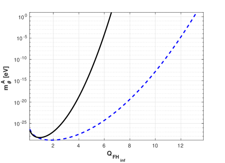
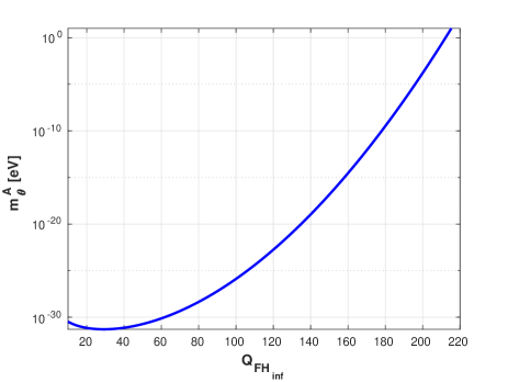
Figure 1: The ALP’s mass value (61) saturating the amplitude of the NANOGrav signal as a function of the ratio $Q_{\rm FH_{\rm inf}}$. Left panel: the solid line corresponds to the initial phase value $\theta_{0}\approx 10^{-2}$ chosen in the vicinity of the origin ($\Delta\theta_{\pi}=\pi$), the dashed line corresponds to $\theta_{0}\approx\pi/2$ ($\Delta\theta_{\pi}=\pi/2$). Right panel: the initial phase value $\theta_{0}$ is taken in the vicinity of $\pi$ ($\Delta\theta_{\pi}=0.1$).

The expression (61) is visualized in Fig.1 as the function of $Q_{\rm FH_{\rm inf}}$, for $C_{A}=1$ and three distinct values of the phase separation, namely $\Delta\theta_{\pi}=\pi/2$ (left panel, dashed line), $\Delta\theta_{\pi}=\pi$ (left panel, solid line) and $\Delta\theta_{\pi}=0.1$ (right panel).

7 Which ALPs may show up in the NANOGrav signal

Let us look at the ALP’s inflationary dynamics related to the NANOGrav signal, as described above, from the point of view of its simultaneous compatibility with constraints on the DM density and isocurvature fluctuations.

In the biggest scale, emerged at the beginning of the inflation, from a single causally connected domain of size $H_{\rm inf}^{-1}$, the ALP field is uniform and frozen at the initial phase value $\theta_{0}$, called misalignment angle. The ALP remains frozen until the equality (52) gets satisfied, which takes place when the temperature of the Universe drops bellow certain value $T_{\rm osc}$. In general, $m_{\theta}$ should depend on the temperature, which, for example, in the case of the QCD axion, is defined by the relation between $T_{\rm osc}$ and $\Lambda$ at which the instanton effects become important (see the most advance lattice calculations in [75]). For ALPs, such kind of dependence should be driven by the details of its gauge couplings and cannot be obtained though a straightforward generalization of the axion case. Bellow, when we quantify the cosmological abundance of ALPs, we treat the mass as being independent of temperature. Our analysis is not sensitive to this assumption.

The total density of ALPs produced in the regime of the inflationary spectator ALP field, namely under the condition (2), is observationally constrained by the CDM density. In particular, in the regime (2), it is required that the mass of ALP and its misalignment angle, defined by $\theta_{0}$, would be mutually fine-tuned. Such kind of fine-tinning can be substantiated with invoking of the anthropic reasoning, which initially has been applied to the QCD axion [18, 19]. The anthropic selection, applied to the QCD axion [18, 19], implies that the misalignment angle should be small ($\theta_{0}<<1$) for PQ symmetry breaking scale relevant for the inflationary QCD axion spectator. In the version of the anthropic selection demanding that any selected variables should have values near the maximal consistent with existence of the human being, the CDM should completely consist of the QCD axions, so that the anthropic window of parameter space is well defined for the QCD axion [18, 19]. However, in this anthropic window a large isocurvature mode is strongly preferred [25, 21, 22, 26], which is at odds with observations, as we discuss bellow. The above constraints apply equaly to QCD axion and ALPs. In particular, a multitude of ALPs is expected to be produced in string theory framework attempting to realize the axion scenario [16, 17, 11], where all ALPs can contribute into CDM content and produce isocurvature perturbations. In this context, it is instructive to investigate, which ALPs from the multitude, possibly existing in string theory, could be seen as the source of stochastic GWs background being able to satisfy the results of ALPs related NANOGrav signal compilation presented in Section 5 and Section 6.

In Section 5 we established that the slope parameter of the spectrum of stochastic GWs generated by the domain walls, created in the ALP inflationary dynamics, exhibits a remarkably good agreement with that one reported by the NANOGrav. Further, we specify the values of the ALP’s scale $F$, its mass $m_{\theta}$ and the misalignment angle $\theta_{0}$ which would lead to the saturation of the NANOGrav signal amplitude (40) simultaneously satisfying the anthropic and isocurvature constrains. In our study, we follow the QCD axion cosmology to describe the origins of the constraints and quote the relevant formulas. Except for the differences due to the treatment of the temperature-dependent mass, the formulas apply equally well for the QCD axion and for ALPs.

When the ALP field starts to oscillate, the ALPs are produced via vacuum misalignment mechanism [3, 4, 5] in form of cold Bose-Einstein condensate with local number density defined by the initial phase value $\theta_{0}$

$$n_{a}\simeq\frac{1}{2}m_{\theta}F^{2}\theta_{0}^{2}f(\theta^{2}),$$ (62)

where $f(\theta^{2})\lesssim 10$ is a correction for anharmonic effects of the axion-like potential. The number density $n_{a}$ red shifts in the same manner as the entropy density, so that

$$\rho_{a}\simeq m_{\theta}s_{0}R_{\gamma}\frac{n_{a}}{s},$$ (63)

where $s=(2\pi^{2}/45)g_{*s}T_{\rm osc}^{3}$ is the thermal entropy density when the oscillations begin, while $s_{0}=(2\pi^{2}/45)g_{*s0}T_{0}^{3}$ is the nowadays entropy density $g_{*s0}=3.91$ and $T_{0}=2.73$K. The factor $R_{\gamma}$ indicates a possible entropy production after the axion begins to oscillate. Eventually, the above outlined misalignment ALPs abundance can be expressed as (see for example [14, 15])

$$\Omega_{\rm ALP}h^{2}\approx 0.12\left(\frac{5\times 10^{-9}\ {\rm eV}}{m_{\theta}}\right)^{1.165}\left(\frac{\theta_{0}}{1.6\times 10^{-2}}\right)^{2}.$$ (64)

This implies, that in the regime when the PQ-like symmetry remains broken during the inflation and afterwards, ALPs in neV mass range will contribute 100% into CDM, provided that the initial phase value obeys $\theta_{0}\lesssim 0.01$. That way, the values of $m_{\theta}$ and $\theta_{0}$ define the anthropic window for the QCD axion and ALPs.

The quantum fluctuations (6) do not alter the local energy density of the ALPs, but instead are imprinted in the fluctuations of the ALPs number density $\delta(n_{a}/s)\neq 0$, called isocurvature fluctuations. Since the ALPs, considered here, are coupled very weakly to the Standard Model (SM) particles , they never come to the thermal equilibrium. In the absence of thermalisation, these fluctuations must be compensated by radiation fluctuations. The amount of ALP-like isocurvature perturbations $\alpha$ is constrained to

$$\alpha=\frac{\langle(\delta T/T)_{\rm iso}^{2}\rangle}{\langle(\delta T/T)_{\rm tot}^{2}\rangle}\lesssim 0.038$$ (65)

at $k=0.05\ {\rm Mpc^{-1}}$, as inferred in [28]. The details of estimation technique of the rate (65), for QCD axion and ALP, are given in [25]. In particular, the relative contribution (65) can be parametrized as follows

$$\alpha=\frac{R_{\rm ALP}^{2}\langle S_{\rm ALP}^{2}(k)\rangle}{R_{\rm ALP}^{2}\langle S_{\rm ALP}^{2}(k)\rangle+\langle{\cal R}^{2}(k)\rangle},$$ (66)

where $R_{\rm ALP}=\Omega_{\rm ALP}/\Omega_{\rm CDM}$, is the ALPs’ fraction of the total CDM content of the Universe, and $\langle{\cal R}^{2}(k)\rangle$ and $\langle S_{\rm ALP}^{2}(k)\rangle$ are the adiabatic and the entropy power spectra, respectively. The curvature power spectrum $\langle{\cal R}^{2}(k)\rangle$, for the adiabatic mode of fluctuations of inflaton reads

$$\langle{\cal R}^{2}(k)\rangle=\frac{2\pi H_{k}^{2}}{k^{3}M_{\rm Pl}^{2}\epsilon_{k}},$$ (67)

where $\epsilon$ is the first inflationary slow-roll parameter [30] and the subscript indicates that the quantities are evaluated at $k=aH_{\rm inf}$. Provided, that the quantum fluctuations of the phase (6), are imprinted with a nearly scale invariant spectrum

$$\langle\delta\theta^{2}(k)\rangle=\frac{2\pi^{2}}{k^{3}}\delta\theta^{2}$$ (68)

one obtains [25]

$$\langle S_{\rm ALP}^{2}(k)\rangle=\left\langle\left(\frac{\delta n_{\rm ALP}}{n_{\rm ALP}}\right)^{2}\right\rangle=4\left\langle\left(\frac{\delta\theta}{\theta}\right)^{2}\right\rangle=\frac{2}{k^{3}\theta_{0}^{2}}Q_{\rm FH_{\rm inf}}^{-2}.$$ (69)

Therefore, the isocurvature contribution (66) can be related to the fundamental inflationary and ALP’s parameters by

$$\alpha\simeq\frac{R_{\rm ALP}^{2}\epsilon_{k}}{\pi\theta_{0}^{2}}\left(\frac{M_{\rm Pl}}{H_{\rm inf}}\right)^{2}Q_{\rm FH_{\rm inf}}^{-2},$$ (70)

where it is assumed that $\alpha\ll 1$, as follows from (65).

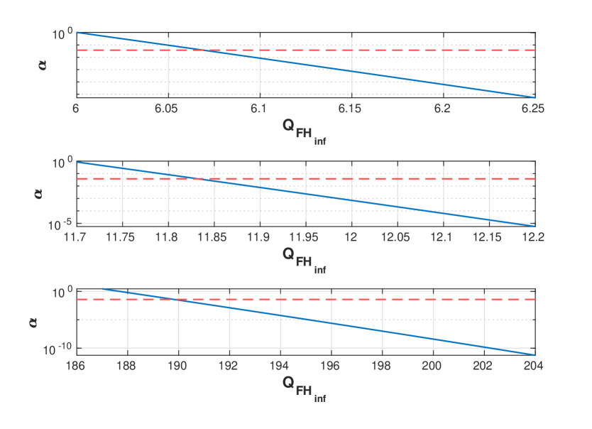
Figure 2: The fraction of ALP-type isocurvature perturbations as the function of $Q_{\rm FH_{\rm inf}}$ (solid line) evaluated under the condition that the ALP mass saturates the NANOGrav signal, as shown in Fig.1. The upper panel corresponds to the initial phase value $\theta_{0}\approx 10^{-2}$ ($\delta\theta_{\pi}\approx\pi$). The middle panel shows the functional dependence for $\theta_{0}=\pi/2$ ($\delta\theta_{\pi}=\pi/2$). The lower panel corresponds to the initial phase value in the vicinity of $\pi$, namely $\theta_{0}=\pi-0.1$ ($\delta\theta_{\pi}=0.1$). The horizontal, dashed line indicates the bound (65), deduced from the Plank measurements.

Taking into account (64), one can express the isocurvature fraction (70) as follows

$$\alpha(m_{\theta},Q_{\rm FH_{\rm inf}},\theta_{0})\approx\left(\frac{5\times 10^{-9}\ {\rm eV}}{m_{\theta}}\right)^{2.33}\left(\frac{\theta_{0}}{1.6\times 10^{-2}}\right)^{4}\left(\frac{M_{\rm Pl}}{H_{\rm inf}}\right)^{2}\frac{\epsilon_{k}}{\pi\theta_{0}^{2}Q_{\rm FH_{\rm inf}}^{2}}$$ (71)

During inflation, the primordial tensor perturbations are generated, setting the initial amplitude for GWs which oscillate after horizon entry. The spectrum of these tensor perturbations is conveniently specified as by the tensor fraction $r=\langle{\cal R}_{T}^{2}(k)\rangle/\langle{\cal R}^{2}(k)\rangle$. In the slow-roll approximation [30]

$$r=16\epsilon$$ (72)

is experimentally bounded to $r<0.058$ [76] (at $k=0.002\ {\rm Mpc^{-1}}$), which we use to estimate the upper limit on the first slow-roll parameter

$$\epsilon_{k}\approx 0.036.$$ (73)

Evaluating (71), under the condition of saturation of the NANOGrav amplitude (40), which implies that $m_{\theta}=m_{\theta}^{A}$ (61), and for the upper bounds (49) and (73), one can frame three scenario in which the ALP might contribute, by its inflationary dynamical induced formation of the domain walls, into the stochastic GWs indicated in the NANOGrav observations.

(i) In the first scenario, the initial value of the phase, during inflation, might be chosen in the vicinity of the origin $\theta_{0}\approx 10^{-2}$ ($\Delta\theta_{\pi}\approx\pi$), which would correspond to the anthropic window usually discussed in the context of the QCD axion. The bound (65), as it is displayed in Fig.2 (upper panel), allows to accommodate ALPs with their inflationary dynamics driven by the ratio

$$Q_{\rm FH_{\rm inf}}\geq 6.1$$ (74)

which corresponds , at bound (49), to

$$F\geq 3.8\times 10^{14}\ {\rm GeV.}$$ (75)

In this scenario, according to (61), as it is shown in left panel of Fig.1, ALP with detectable domain walls GWs signature should have mass

$$m_{\theta}\gtrsim 10^{-4}\ {\rm eV}$$ (76)

and contribute, as it follows from (64),

$$R_{\rm ALP}\lesssim 10^{-5}$$ (77)

of the total CDM content of the Universe. Eventually, applying (8), one obtains the value of the stress energy density of the domain walls

$$\sigma\gtrsim 5.8\times 10^{16}\ {\rm GeV^{3}}.$$ (78)

(ii) The second scenario assumes that the initial phase value $\theta_{0}=\pi/2$ (that is $\mathcal{O}(1)$), and, as it is shown in Fig.2 (middle panel), accommodates the ALP with ratio

$$Q_{\rm FH_{\rm inf}}\geq 11.9,$$ (79)

which corresponds to

$$F\geq 7.0\times 10^{14}\ {\rm GeV.}$$ (80)

In this scenario, the ALP with detectable domain walls implies

$$m_{\theta}\gtrsim 1.2\times 10^{-5}\ {\rm eV},$$ (81)

as it follows from (61) (see left panel of Fig.1). Thus, according to (64)

$$R_{\rm ALP}\lesssim 1,$$ (82)

which implies that the ALPs constitutes total CDM budget of the Universe. The value of the stress energy of the domain walls reads

$$\sigma\gtrsim 2.3\times 10^{16}\ {\rm GeV^{3}}.$$ (83)

(iii) In the third scenarios, we put the initial phase value to $\theta_{0}=\pi-0.1$ ($\Delta\theta_{\pi}=0.1$), which implies the initial phase position $\theta_{0}$ in a vicinity of the domain wall formation crossing point. Thus, the isocurvature bound (65), as shown in lower panel of Fig.2, can accommodate the ALP with ratio

$$Q_{\rm FH_{\rm inf}}\geq 189.8,$$ (84)

which would correspond to the ALP mass, saturating the NANOGrav signal amplitude (see Fig.1, right panel),

$$m_{\theta}\gtrsim 1.7\times 10^{-7}\ {\rm eV}.$$ (85)

However, according to (64), the ALPs with such mass and initial phase, in the vicinity of $\pi$, are definitely overabundant. If we increase the mass limit up to

$$m_{\theta}\gtrsim 4\times 10^{-5}\ {\rm eV},$$ (86)

which implies that (see Fig.1, right panel)

$$Q_{\rm FH_{\rm inf}}\geq 198.2$$ (87)

and

$$F\geq 1.2\times 10^{16}\ {\rm GeV},$$ (88)

the ALPs will constitute the total CDM content of the Universe ($R_{\rm ALP}\lesssim 1$) and give a negligible contribution into the ALP-like isocurvature fraction, which reads

$$\alpha\lesssim 7\times 10^{-8}.$$ (89)

In this case, one expects the highest possible value of the stress energy density of the domain walls, namely

$$\sigma\gtrsim 5.7\times 10^{18}\ {\rm GeV^{3}}.$$ (90)

Thus, in the context of detectability of ALPs from their multitude, possibly produced in string theory [16, 17, 11] along with the QCD axion, one infers the following. If one of the ALPs has the misalignment angle value set to the same one, $\theta_{0}\approx 10^{-2}$, imposed by the anthropic window of the QCD axion, it may saturate the NANOGrav excess amplitude even having a negligible contribution into the CDM density (77), at the same time being consistent with the isocurvature constraint. If one of the ALPs has large value of the misalignment angle, $\theta_{0}\approx 1$, it should dominate the CDM density (82) and the isocurvature contributions to be interpreted as the source of the saturation of the NANOGrav amplitude. In case of one of the ALPs has $\theta_{0}$ value very close to $\pi$, which is, however, as probable as the QCD axion anthropically selected $\theta_{0}$, it may manifest itself in the NANOGrav, in the condition of the dominant contribution into the CDM density and negligible contribution into the isocurvature perturbations (89). However, in this case, instead of collapsing the domain walls of NANOGrav scale range should form wormholes, as we elucidate in Section 8.

Let us notice that, according to (113), at $N\approx 60$, the domain wall formation crossing point is reached within almost 100% of the horizon exiting scales, for each of three above considered scenario. However, these scales, corresponding to the very end of inflation, are definitely much smaller than the width of domain walls typical for the scenario described above, so that the dynamics of the resulting vacuum-like objects should be much different than that one of the domain walls discussed above.

8 Domain walls escaping into baby universes

Walls of size $R(t_{H})=H^{-1}$ cross the Hubble radius defined by the Hubble rate $H=\dot{a}/a$. The mass of a wall at Hubble crossing is expressed as

$$M_{\rm w}(H)\approx 4\pi\sigma H^{-2}=4\pi M_{\rm Pl}\left(\frac{\sigma}{M_{\rm Pl}^{3}}\right)\left(\frac{M_{\rm Pl}}{H}\right)^{2}.$$ (91)

Once the wall becomes encompassed by a Hubble radius it collapses, within about a Hubble time, into a PBH of mass $M_{\rm PBH}=\xi M_{\rm w}$, where $\xi\simeq 1$ indicates the fraction of the wall energy deposited into the BH. The wall stress energy tension is a source of repulsive gravity [58, 64, 65, 68] and hence should maintain a negative pressure in case of a domination of the wall’s material inside of encompassing it Hubble radius. The collapse can take place unless the the mass of the wall inside a given Hubble radius exceed the mass of its matter content which happens when the Hubble rate reaches the value

$$H_{\rm w}\approx 8\pi\sigma G=8\pi M_{\rm Pl}\left(\frac{\sigma}{M_{\rm Pl}^{3}}\right).$$ (92)

Thus, for stress energy density (90) relevant for the ALP parameters localized in scenario (iii), discussed in Section 7, the dominating wall “enters”  the horizon at Hubble rate $H_{\rm w(iii)}\approx 10^{-9}\ {\rm eV}$. Comparing this rate with that one at which $f_{\rm yr}$ enters into Hubble radius (54) one can see that the walls of size corresponding to the frequencies $f_{\rm w(iii)}\gtrsim 300$ nHz are able to collapse into PBHs. Bigger walls entered the Hubble radius starts expanding faster than the background reaching eventually the inflationary vacuum and develop wormholes to baby universes [61, 62]. Such wormholes are seen as BHs in the FRW Universe. Since this frequency is much higher than the frequencies of the signal bins of the NANOGrav, the ALP domain walls, described in (iii), should mostly form wormholes. Provided that the condition (51) fails in each scenario of Section 7, the acoustic response signal (50) induced by these escaping walls cannot saturate the amplitude (28). Therefore, most likely the ALP field with parameters specified in scenario (iii) cannot be a source of the signal indicated by the NANOGrav.

In scenarios (i) and (ii), the dominating wall enters the horizon at Hubble rate $H_{\rm w(i)}\approx 10^{-11}\ {\rm eV}$, which corresponds to the GW signal frequency of $f_{\rm w(i)}\lesssim 3$ nHz. Therefore, the domain walls induced by inflationary dynamics of the ALP fields specified in scenarios (i) and (ii) should collapse into PBHs within almost the whole range of frequency support of the NANOGrav. The slope of the strain spectrum (44), which might be generated by these walls, $\gamma=5.5$, exhibits a remarkable agreement with the central value of the slope range (41) reported by NANOGrav [42], in its excess frequency bins. Generically, it would be reasonable to expect a sort of spectral feature expressed as the slope change from $\gamma=3.5$, for frequencies bellow $f_{\rm w(i)}\simeq 3$ nHz to $\gamma=5.5$ for higher frequencies. Such kind of feature might indicate the transition from the regime when bigger walls, “entering” their Hubble radii, were escaping into baby universes and those smaller ones which were collapsing into PBHs. However, because of the amplitude inconsistency between collapsing (44) and escaping (50) strains, caused by the violation of condition (51),  one might expect to see only a spectrum of slope $\gamma=5.5$ with amplitude almost abruptly attenuating at frequencies bellow $f_{\rm w(i)}\simeq 3$ nHz.

Currently, NANOGrav has about $T\approx 15$ years of high precision timing observations from many pulsars, where every pulsar is observed each $\Delta t\simeq 1\div 3$ weeks with integration time about 20 minutes. Thus, the sensitivity band to GW frequency can be defined as $1/T<f<\Delta t/2$, which spans the range from $\simeq 2$ nHz to $\simeq 1\ {\rm\mu Hz}$. This means, that in scenarios (i) and (ii), the frequency range indicating the domain walls forming wormholes, may be, just barely reaches the lowest frequency bin accessible for the NANOGrav. Therewith, it would be hard to expect to obtain a real testification on wormholes formation by ALP field induced domain walls.

The boundary between a PBH collapsing and wormhole escaping domain wall can be characterized by the mass of wall material contained within the size $H_{\rm w}$, which reads

$$M_{\rm w}(H_{\rm w})\approx\frac{M_{\rm Pl}}{16\pi}\left(\frac{M_{\rm Pl}^{3}}{\sigma}\right).$$ (93)

For the parameters specified for the NANOGrav detectable ALPs, the values of the boundary mass are $M_{\rm w(i)}\approx 7{\rm M_{\odot}}$ in scenario (i), $M_{\rm w(ii)}\approx 18{\rm M_{\odot}}$ in scenario (ii) and $M_{\rm w(iii)}\approx 0.07{\rm M_{\odot}}$ in scenario (iii). These values indicate the upper bounds of PBH mass formed by collapsing domain walls. The heavier BHs are induced by domain walls developing wormholes, so that their masses cannot exceed the energy of the radiation fluid contained in a respective Hubble radius [61], provided that horizon entering took place before the equality epoch.

Closing the section, we notice, that the observational access to the signature of domain walls escaping into baby universes may be more encouraging in the context of the spontaneous nucleation of domain walls on the inflationary stage, considered in [63, 61, 62]. In this setup, the nucleation rate $\Gamma_{s}\propto\exp(-S_{E})$ is defined by the action $S_{E}$ of the semi-classical tunneling pass, $S_{E}\simeq 2\pi^{2}\sigma H_{\rm inf}^{-3}$. To instance, for higher reference frequency $f_{0}>f_{\rm yr}$, one may represent (50) as

$$h_{c{\rm b}}(f)=0.55\kappa\sqrt{\Gamma_{s}}\left(\frac{f_{\rm yr}}{f_{0}}\right)^{\frac{1}{4}}\left(\frac{f}{f_{\rm yr}}\right)^{-\frac{1}{4}}.$$ (94)

Therefore, the signature of domain wall escaping into baby universes might be seen with a detector of GWs having sensitive to amplitude

$$A_{B}^{0}\lesssim 0.3\kappa^{2}\Gamma_{s}\left(\frac{f_{\rm yr}}{f_{0}}\right)^{\frac{1}{2}}$$ (95)

in the characteristic strain power spectrum like (39), measuring the slope value to be close to that one of the acoustic response, $\gamma=3.5$. Presumably, Gaia and THEIA can have some potential to provide sensitive measurements in much higher frequency band [77].

9 Consistency of collapsing walls evolution with PBHs constraints

There is no domain wall problem related to their production mechanism considered in this paper. The walls which create wormholes export the domain wall problem into baby universes. The collapsing walls form PBHs before their contribution into the energy density becomes large enough to contradict the observational constraints.

The dynamics of spherical domain wall has been studied in [64]. The result of this study implies that a closed domain wall being initially bigger than its Schwartzshild radius always collapses into a BH. Thus, the ALP field induced domain wall after obtaining of a spherical geometry contracts toward the center. Since the ALP’s coupling to the Standard Model particles is strongly suppressed by the large scale $F$, so that the ALP wall interacts very weakly with matter and hence nothing can prevent the wall finally to be localized within a volume of size comparable to its width [32, 33]. The Schwarzschild radius of a wall of total mass $M_{\rm w}$

$$R_{\rm S}=2GM_{\rm w}$$ (96)

can be expressed trough the radius of the wall $R_{\rm w}$ and the ALP parameters as follows

$$R_{\rm S}=32\pi GR_{\rm w}^{2}m_{\theta}F^{2}.$$ (97)

Provided that the wall contracts down to about the size comparable to its width $\simeq m_{\theta}^{-1}$, one naturally assumes that a PBH will be formed under the condition $R_{\rm S}>m_{\theta}^{-1}$, which reads

$$R_{\rm w}>\frac{m_{\theta}^{-1}}{4\sqrt{2\pi}}\frac{M_{\rm Pl}}{F}$$ (98)

Since, the NANOGrav frequencies would correspond to the size of the emitting object

$$R_{\rm w}\simeq\frac{f_{\rm yr}^{-1}}{1+z_{\rm osc}},$$ (99)

one can impose the following constraint on the ALP’s mass

$$m_{\theta}\gtrsim\frac{32\pi}{\sqrt{\Omega_{\rm r}}}f_{\rm yr}\left(\frac{f_{\rm yr}}{H_{0}}\right)\left(\frac{M_{\rm Pl}}{F}\right)^{2}\approx 8.2\times 10^{-16}\left(\frac{M_{\rm Pl}}{F}\right)^{2}\ {\rm eV},$$ (100)

where we used (53) to evolve (98) and (99). The numerical value of the constraint (100) reads $m_{\theta{\rm(i)}}\approx 8.5\times 10^{-7}$ eV, $m_{\theta{\rm(ii)}}\approx 2.5\times 10^{-7}$ eV and $m_{\theta{\rm(ii)}}\approx 8.5\times 10^{-10}$ eV for scenario (i), (ii) and (iii) respectively. Thus, one can affirm that in all three scenarios described in Section 7, the condition (100) is well satisfied, which implies that the domain walls producing GWs signals of frequencies about $f_{\rm yr}$, are capable to deposit their energy under their Schwarzschild radius and hence convert it into PBHs. It is obvious, that the above statement is still in tact also for frequencies one order of magnitude bellow and above $f_{\rm yr}$.

In what follows, we verify the consistency of PBHs abundance of different masses produced by collapsing closed domain walls, with existing constraints [40].

The mass distribution of the BHs is defined by the size distribution of the walls’ seeding contours (13) scaled with respect to the expansion of the Universe, which is given in (23) and reads as

$$dn=\Gamma_{s}\frac{dR}{t_{eq}^{3/2}R^{5/2}},$$ (101)

at the equality time. A useful characteristic of this distribution, which allows to compare the PBHs yield with the constraints on their abundance in different mass range [40] , is the mass density of PBHs per logarithmic mass interval in units of the total density of the Universe

$$\frac{d\Omega_{\rm PBH}}{d\ln M_{\rm PBH}}=\frac{1}{\rho_{eq}}\frac{dn}{d\ln M_{\rm PBH}}M_{\rm PBH},$$ (102)

where $\rho_{\rm eq}=M_{\rm Pl}^{2}/(6\pi t_{\rm eq}^{2})$ is the matter density at the time of equality. Using (101), we can obtain

$$\frac{dn}{d\ln M_{\rm PBH}}=\frac{\Gamma_{s}}{2}\frac{1}{t_{eq}^{3/2}}(4\pi\sigma)^{3/4}M_{\rm PBH}^{-3/4},$$ (103)

so that (102) can be converted into

$$\frac{d\Omega_{\rm PBH}}{d\ln M_{\rm PBH}}=\frac{3\pi\Gamma_{s}t_{\rm eq}^{1/2}(4\pi\sigma)^{3/4}M_{\rm PBH}^{1/4}}{M_{\rm Pl}^{2}},$$ (104)

to be compared with the model

$$\Omega_{\rm PBH}\sim 10^{9}\beta\left(\frac{M_{\rm PBH}}{M_{\odot}}\right)^{-1/2}$$ (105)

used in [40] to quote the constraints on the density fraction $\beta$ deposited in PBHs at the moment of their formation. In particular, independently of the NANOGrav signal, one can provide an upper bound, shown in the left panel of Fig. 3, on the combination $\sigma\Gamma_{s}^{4/3}$ for PBHs of different masses formed in a domain walls collapse process, provided that each wall converts its total mass into a PBH. One can see that the restrictions (see left panel in Fig. 3) become gap-like tougher, namely $\sigma\Gamma_{s}^{4/3}\leq 10^{-7}$, in a range of masses exceeding the boundary mass $M_{\rm w}(H_{\rm w})=17M_{\odot}$ quoted above.

Figure 3: Left panel: Constraints on the combination of parameters $\sigma\Gamma_{s}^{4/3}$ based on the known constraints on primordial black holes [40]. Right panel: The solid curve corresponds to the observed NANOGrav frequency $f_{0}=2.5$ nHz, the dashed curve corresponds to $f_{0}=12$ nHz. The straight line shows the NANOGrav driven correlation (110) for $C_{A}=1$. The double side arrow sign corresponds to the range of the domain walls stress energy defined in scenarios (i)-(iii) of Section 7.

In general, the relation (91) implies that different combinations of $R$ and $\sigma$ may be composed into one and the same mass of the PBH. This degeneracy is removed if we fix the reference frequency $f_{\rm yr}$ of the NANOGrav signal. Thus, using the chain of relations (104), (91), $R=ct$,

$$1/t=f=f_{\rm yr}(1+z),$$ (106)

and the connection

$$1+z=(1+z_{\rm eq})t_{\rm eq}^{1/2}/t^{1/2}$$ (107)

one arrives to

$$\sigma=\frac{M_{\rm PBH}f_{0}^{4}t_{\rm eq}^{2}(1+z_{\rm eq})^{4}}{4\pi},$$ (108)

and

$$\Gamma_{s}=\frac{(d\Omega_{\rm PBH}/d\ln M_{\rm PBH})M_{\rm Pl}^{2}}{3\pi t_{\rm eq}^{2}M_{\rm PBH}f_{0}^{3}(1+z_{\rm eq})^{3}}.$$ (109)

The expressions (108) and (109) together with constraints presented in [40] impose the bound on $\Gamma_{s}$, which is shown by dogleg lines in the right panel of Fig. 3.

Using (44) and (40) one can infer the mutual correlation which NANOGrav signal imposes on $\sigma$ and $\Gamma_{s}$, in case of saturation of the signal amplitude

$$\log\Gamma_{s}=2\log C_{\rm A}-15.4-2\log\left(\frac{\sigma}{1{\rm GeV}^{3}}\right)$$ (110)

This equation is shown by the straight line in the right panel of Fig. 3.

Thus, one can see that the PBHs contribution from the collapsing ALP domain walls saturating with their GWs emission the NANOGrav signal is well bellow the allowed limit on the PBHs abundance.

10 Conclusions

In this paper, we have explored the impact of the evolution of closed domain walls, created in course of dynamics of ALP field spectating the inflation, on the stochastic GWs background in the frequency range accessible for the PTA measurements.

As long as the Universe is inflating, an axion or ALP field owing, by definition, the discrete set of vacuum states, with PQ (-like) symmetry broken before inflation, experiences the quantum fluctuations. In some patches of the space, an accumulation of the fluctuations can move the field, from its initial value (misalignment angle), so much that after inflation it will be located in a vacuum state differing from that one corresponding to its value occurred at the beginning of the inflation. Thus, due to inflationary expansion and provided that the probability for the field to acquire the value corresponding to another vacuum state is small enough, one expects to see a Swiss cheese like picture where the domains with underrepresented vacuum will be inserted into a space remaining filled with the initial one. Two different neighboring vacuum states should be interpolated by a domain wall, represented by the sine-Gordon kink solution (7) in the case of axions or ALPs. Obviously, the Swiss cheese structure guaranties that the produced domain walls have closed, although irregular, shapes .

Evolving after inflation, the domain walls, depending on their sizes, either collapse forming PBHs or escape into baby universes leaving wormholes anyway observed as BHs in our Universe. Therethrough, there is no domain wall problem in either scenario.

The collapsing walls tend to decrease their entropy leading to a smoothing out of their surfaces, and hence radiating our the energy in form of GWs, with characteristic frequency of about the Hubble rate established during their collapsing instants. We have estimated the characteristic strain power spectrum produced by the size distribution of the collapsing closed domain walls and relate it with the recently reported NANOGrav signal excess obtained in PTA measurements. It is remarkable, that the slope of the frequency dependence of the strain spectrum $\gamma=5.5$, generated by such domain walls, is very well centered inside the range of the slopes in the signal obtained by the NANOGrav.

Analyzing the inflationary dynamics of the ALP field, in consistency with the isocurvature constraint, we defined those combinations of its parameters where the signal from the inflationary induced ALPs domain walls could saturate the amplitude of the NANOGrav excess. In particular, if an ALP has the misalignment angle value set to the same one, imposed by the anthropic window of the QCD axion, it may saturate the NANOGrav excess amplitude even having a negligible contribution into the CDM density, at the same time being consistent with the isocurvature constraint. Provided that string theory models that include the QCD axion, generically at high scale of PQ symmetry breaking, might also incorporate other ALPs which can leave their imprint in the stochastic GWs background, with the preferred by the NANOGrav excess parameters of the characteristic strain power spectrum and without overproduction of CDM and/or isocuvature modes.

Those walls exceeding by their mass the energy of the bulk fluid inside the Hubble radius will dominate by their repulsive nature and hence push the fluid away, leaving two nearly empty layers in their vicinity. Such walls, keeping exponentially extending, escape into baby universes forming wormholes in our Universe, which are observed as BHs of masses ranging from planetary to some of LIGO/Virgo scales [80, 81], depending on the parameters of ALPs. We assumed that being pushed away the bulk radiation fluid responds by acoustics waves which may set in a motion a fraction of the mass in Hubble radius. This mass, in a motion, could generate the GWs signal with the strain spectrum slope and the amplitude different from that ones expected from the collapsing walls. It was found that in the context of domain walls produces by ALPs, it is quite unlikely, while in principle possible, to trace baby universes in PTA measurements. However, a detectable stochastic GWs imprint of the phenomena can be specified for other types of phase transitions which might occur during inflation.

At some final inflationary e-folds, corresponding to much smaller than the NANOGrav scales, the probability of the ALP field to move its value into another vacuum may become large, which may correspond to percolated domain walls system considered in [82] and induce small scale density inhomogeneities in the distribution of the coherent oscillations of the ALPs Bose-Eisenstein condensate. Possible scenarios of evolution and observational signatures of small scale inhomogeneities in axionic Bose-Eisenstein condensate have been studied in great details in the cosmology of QCD axion (see for example [83, 84, 85, 86, 87, 88]).

Appendix A First passage e-fold

Providing the condition $p(\Delta\theta_{\pi},N)\approx 1$, in (57), one can define how many e-folds would it take the phase to cross $\pi$, solving the following equation

$$3N_{\pi}^{2}+(\frac{1}{2}\ln 2\pi+\ln\Delta\theta_{\pi}+\ln Q_{\rm FH_{\rm inf}}-\frac{3}{2}\ln N_{\pi})N_{\pi}-2\pi^{2}\Delta\theta_{\pi}^{2}Q_{\rm FH_{\rm inf}}^{2}=0.$$ (111)

One can put the term $\frac{3}{2}\ln N$ in the parenthesis to a constant $C_{1}\approx 4.5\div 6.2$, provided that it changes quite slow with increasing of $N$ in the range $N\approx 20\div 60$. Under this assumption, the solution of (111) can be approximated by the root of quadratic equation, given by

$$N_{\pi}\approx\frac{(24\pi^{2}\Delta\theta_{\pi}^{2}Q_{\rm FH_{\rm inf}}^{2}-(0.9\ln\Delta\theta_{\pi}+\ln Q_{\rm FH_{\rm inf}}-C_{1}))^{1/2}}{6}-\frac{(0.9\ln\Delta\theta_{\pi}+\ln Q_{\rm FH_{\rm inf}}-C_{1})^{2}}{6}.$$ (112)

For reasonable choose of parameter, $1<Q_{\rm FH_{\rm inf}}\lesssim 10$ and $\Delta\theta_{\pi}\simeq\pi/2$ and provided that typically accepted number of e-folds needed for inflation $N_{\rm inf}\simeq 60$, one can neglect relevant terms in (112), so that the solution is reduced to

$$N_{\pi}\approx\pi\Delta\theta_{\pi}Q_{\rm FH_{\rm inf}}.$$ (113)

References

- [1] R. D. Peccei and H. R. Quinn, “CP Conservation in the Presence of Instantons,” Phys. Rev. Lett. 38 (1977), 1440-1443 doi:10.1103/PhysRevLett.38.1440
- [2] R. D. Peccei and H. R. Quinn, “Constraints imposed by CP conservation in the presence of pseudoparticles,” Phys. Rev. D16 (1977), 1791-1797
- [3] L. F. Abbott and P. Sikivie, “A Cosmological Bound on the Invisible Axion,” Phys. Lett. B 120 (1983), 133-136 doi:10.1016/0370-2693(83)90638-X
- [4] M. Dine and W. Fischler, “The Not So Harmless Axion,” Phys. Lett. B 120 (1983), 137-141 doi:10.1016/0370-2693(83)90639-1
- [5] J. Preskill, M. B. Wise and F. Wilczek, “Cosmology of the Invisible Axion,” Phys. Lett. B 120 (1983), 127-132 doi:10.1016/0370-2693(83)90637-8
- [6] J. E. Kim, “Light Pseudoscalars, Particle Physics and Cosmology,” Phys. Rept. 150 (1987), 1-177 doi:10.1016/0370-1573(87)90017-2
- [7] D. J. E. Marsh, “Axion Cosmology,” Phys. Rept. 643 (2016), 1-79 doi:10.1016/j.physrep.2016.06.005 [arXiv:1510.07633 [astro-ph.CO]].
- [8] L. Di Luzio, M. Giannotti, E. Nardi and L. Visinelli, “The landscape of QCD axion models,” Phys. Rept. 870 (2020), 1-117 doi:10.1016/j.physrep.2020.06.002 [arXiv:2003.01100 [hep-ph]].
- [9] P. Sikivie, “Axion Cosmology,” Lect. Notes Phys. 741 (2008), 19-50 doi:10.1007/978-3-540-73518-2_2 [arXiv:astro-ph/0610440 [astro-ph]].
- [10] S. Chang, C. Hagmann and P. Sikivie, “Studies of the motion and decay of axion walls bounded by strings,” Phys. Rev. D 59 (1999), 023505 doi:10.1103/PhysRevD.59.023505 [arXiv:hep-ph/9807374 [hep-ph]].
- [11] A. Arvanitaki, S. Dimopoulos, S. Dubovsky, N. Kaloper and J. March-Russell, “String Axiverse,” Phys. Rev. D 81 (2010), 123530 doi:10.1103/PhysRevD.81.123530 [arXiv:0905.4720 [hep-th]].
- [12] P. Arias, D. Cadamuro, M. Goodsell, J. Jaeckel, J. Redondo and A. Ringwald, “WISPy Cold Dark Matter,” JCAP 06 (2012), 013 doi:10.1088/1475-7516/2012/06/013 [arXiv:1201.5902 [hep-ph]].
- [13] A. Ringwald, “Exploring the Role of Axions and Other WISPs in the Dark Universe,” Phys. Dark Univ. 1 (2012), 116-135 doi:10.1016/j.dark.2012.10.008 [arXiv:1210.5081 [hep-ph]].
- [14] G. Ballesteros, J. Redondo, A. Ringwald and C. Tamarit, “Standard Model—axion—seesaw—Higgs portal inflation. Five problems of particle physics and cosmology solved in one stroke,” JCAP 08 (2017), 001 doi:10.1088/1475-7516/2017/08/001 [arXiv:1610.01639 [hep-ph]].
- [15] L. Di Luzio, A. Ringwald and C. Tamarit, “Axion mass prediction from minimal grand unification,” Phys. Rev. D 98 (2018) no.9, 095011 doi:10.1103/PhysRevD.98.095011 [arXiv:1807.09769 [hep-ph]].
- [16] P. Svrcek and E. Witten, “Axions In String Theory,” JHEP 06 (2006), 051 doi:10.1088/1126-6708/2006/06/051 [arXiv:hep-th/0605206 [hep-th]].
- [17] J. P. Conlon, “The QCD axion and moduli stabilisation,” JHEP 05 (2006), 078 doi:10.1088/1126-6708/2006/05/078 [arXiv:hep-th/0602233 [hep-th]].
- [18] A. D. Linde, “Axions in inflationary cosmology,” Phys. Lett. B 259 (1991), 38-47 doi:10.1016/0370-2693(91)90130-I
- [19] M. Tegmark, A. Aguirre, M. Rees and F. Wilczek, “Dimensionless constants, cosmology and other dark matters,” Phys. Rev. D 73 (2006), 023505 doi:10.1103/PhysRevD.73.023505 [arXiv:astro-ph/0511774 [astro-ph]].
- [20] K. J. Mack, “Axions, Inflation and the Anthropic Principle,” JCAP 07 (2011), 021 doi:10.1088/1475-7516/2011/07/021 [arXiv:0911.0421 [astro-ph.CO]].
- [21] J. Hamann, S. Hannestad, G. G. Raffelt and Y. Y. Y. Wong, “Isocurvature forecast in the anthropic axion window,” JCAP 06 (2009), 022 doi:10.1088/1475-7516/2009/06/022 [arXiv:0904.0647 [hep-ph]].
- [22] K. J. Mack and P. J. Steinhardt, “Cosmological Problems with Multiple Axion-like Fields,” JCAP 05 (2011), 001 doi:10.1088/1475-7516/2011/05/001 [arXiv:0911.0418 [astro-ph.CO]].
- [23] D. H. Lyth, “Axions and inflation: Sitting in the vacuum,” Phys. Rev. D 45 (1992), 3394-3404 doi:10.1103/PhysRevD.45.3394
- [24] D. H. Lyth and E. D. Stewart, “Constraining the inflationary energy scale from axion cosmology,” Phys. Lett. B 283 (1992), 189-193 doi:10.1016/0370-2693(92)90006-P
- [25] M. Beltran, J. Garcia-Bellido and J. Lesgourgues, “Isocurvature bounds on axions revisited,” Phys. Rev. D 75 (2007), 103507 doi:10.1103/PhysRevD.75.103507 [arXiv:hep-ph/0606107 [hep-ph]].
- [26] L. Visinelli, “Light axion-like dark matter must be present during inflation,” Phys. Rev. D 96 (2017) no.2, 023013 doi:10.1103/PhysRevD.96.023013 [arXiv:1703.08798 [astro-ph.CO]].
- [27] S. Kasuya and M. Kawasaki, “Axion isocurvature fluctuations with extremely blue spectrum,” Phys. Rev. D 80 (2009), 023516 doi:10.1103/PhysRevD.80.023516 [arXiv:0904.3800 [astro-ph.CO]].
- [28] Y. Akrami et al. [Planck], “Planck 2018 results. X. Constraints on inflation,” Astron. Astrophys. 641 (2020), A10 doi:10.1051/0004-6361/201833887 [arXiv:1807.06211 [astro-ph.CO]].
- [29] A. D. Linde, “Particle physics and inflationary cosmology,” Contemp. Concepts Phys. 5 (1990), 1-362 [arXiv:hep-th/0503203 [hep-th]].
- [30] A.R. Liddle and D.H. Lyth, Cosmological Inflation and Large-Scale Structure, (Cambridge University Press, Cambridge, England, 2000)
- [31] D. H. Lyth and E. D. Stewart, “Axions and inflation: String formation during inflation,” Phys. Rev. D 46 (1992), 532-538 doi:10.1103/PhysRevD.46.532
- [32] S. G. Rubin, M. Y. Khlopov and A. S. Sakharov, “Primordial black holes from nonequilibrium second order phase transition,” Grav. Cosmol. 6 (2000), 51-58 [arXiv:hep-ph/0005271 [hep-ph]].
- [33] M. Y. Khlopov, S. G. Rubin and A. S. Sakharov, “Primordial structure of massive black hole clusters,” Astropart. Phys. 23 (2005), 265 doi:10.1016/j.astropartphys.2004.12.002 [arXiv:astro-ph/0401532 [astro-ph]].
- [34] Y. B. Zeldovich, I. D. Novikov, “The hypothesis of cores retarded during expansion and the hot cosmologica lmodel,” Sov. Astron. 10 (1967),10, 602
- [35] S. Hawking, “Gravitationally collapsed objects of very low mass,” Mon. Not. Roy. Astron. Soc. 152 (1971), 75
- [36] B. J. Carr and S. W. Hawking, “Black holes in the early Universe,” Mon. Not. Roy. Astron. Soc. 168 (1974), 399-415
- [37] M. Y. Khlopov and A. G. Polnarev, “Primordial black holes as a cosmological test of grand unification,” Phys. Lett. B 97 (1980), 383-387 doi:10.1016/0370-2693(80)90624-3
- [38] A. G. Polnarev and M. Y. Khlopov, “Cosmology, primordial black holes, and supermassive particles” Sov. Phys. Usp. 28 (1985), 213-232 doi:10.1070/PU1985v028n03ABEH003858
- [39] M. Y. Khlopov, “Primordial Black Holes,” Res. Astron. Astrophys. 10 (2010), 495-528 doi:10.1088/1674-4527/10/6/001 [arXiv:0801.0116 [astro-ph]].
- [40] B. Carr, K. Kohri, Y. Sendouda and J. Yokoyama, “Constraints on Primordial Black Holes,” [arXiv:2002.12778 [astro-ph.CO]].
- [41] K. M. Belotsky, V. I. Dokuchaev, Y. N. Eroshenko, E. A. Esipova, M. Y. Khlopov, L. A. Khromykh, A. A. Kirillov, V. V. Nikulin, S. G. Rubin and I. V. Svadkovsky, “Clusters of primordial black holes,” Eur. Phys. J. C 79 (2019) no.3, 246 doi:10.1140/epjc/s10052-019-6741-4 [arXiv:1807.06590 [astro-ph.CO]].
- [42] Z. Arzoumanian et al. [NANOGrav], “The NANOGrav 12.5-year Data Set: Search For An Isotropic Stochastic Gravitational-Wave Background,” [arXiv:2009.04496 [astro-ph.HE]].
- [43] M.V. Sazhin, “Opportunities for detecting ultralong gravitational waves”, Soviet Astronomy, 22, (1978), 36-38; Translation. Astronomicheskii Zhurnal, 55, (1978), 65-68.
- [44] S. L. Detweiler, “Pulsar timing measurements and the search for gravitational waves,” Astrophys. J. 234 (1979), 1100-1104 doi:10.1086/157593
- [45] R.W. Hellings and G.S. Downs, “Upper limits on the isotropic gravitational radiation background from pulsar timing analysis,” Astrophys. J. Lett. 265 (1983), L39-L42 doi:10.1086/183954
- [46] J. Ellis and M. Lewicki, “Cosmic String Interpretation of NANOGrav Pulsar Timing Data,” [arXiv:2009.06555 [astro-ph.CO]].
- [47] S. Blasi, V. Brdar and K. Schmitz, “Has NANOGrav found first evidence for cosmic strings?,” [arXiv:2009.06607 [astro-ph.CO]].
- [48] W. Buchmuller, V. Domcke and K. Schmitz, “From NANOGrav to LIGO with metastable cosmic strings,” [arXiv:2009.10649 [astro-ph.CO]].
- [49] R. Samanta and S. Datta, “Gravitational wave complementarity and impact of NANOGrav data on gravitational leptogenesis: cosmic strings,” [arXiv:2009.13452 [hep-ph]].
- [50] N. Ramberg and L. Visinelli, “QCD axion and gravitational waves in light of NANOGrav results,” Phys. Rev. D 103 (2021) no.6, 063031 doi:10.1103/PhysRevD.103.063031 [arXiv:2012.06882 [astro-ph.CO]].
- [51] Y. Nakai, M. Suzuki, F. Takahashi and M. Yamada, “Gravitational Waves and Dark Radiation from Dark Phase Transition: Connecting NANOGrav Pulsar Timing Data and Hubble Tension,” [arXiv:2009.09754 [astro-ph.CO]].
- [52] A. Addazi, Y. F. Cai, Q. Gan, A. Marciano and K. Zeng, “NANOGrav results and Dark First Order Phase Transitions,” [arXiv:2009.10327 [hep-ph]].
- [53] J. Liu, R. G. Cai and Z. K. Guo, “Large anisotropies of the stochastic gravitational wave background from cosmic domain walls,” [arXiv:2010.03225 [astro-ph.CO]].
- [54] A. Paul, U. Mukhopadhyay and D. Majumdar, “Gravitational Wave Signatures from Domain Wall and Strong First-Order Phase Transitions in a Two Complex Scalar extension of the Standard Model,” [arXiv:2010.03439 [hep-ph]].
- [55] A. Neronov, A. Roper Pol, C. Caprini and D. Semikoz, “NANOGrav signal from MHD turbulence at QCD phase transition in the early universe,” [arXiv:2009.14174 [astro-ph.CO]].
- [56] A. Brandenburg, E. Clarke, Y. He and T. Kahniashvili, “Can we observe the QCD phase transition-generated gravitational waves through pulsar timing arrays?,” [arXiv:2102.12428 [astro-ph.CO]].
- [57] S. Vagnozzi, “Implications of the NANOGrav results for inflation,” Mon. Not. Roy. Astron. Soc. 502 (2021) no.1, L11-L15 doi:10.1093/mnrasl/slaa203 [arXiv:2009.13432 [astro-ph.CO]].
- [58] A. Vilenkin and E. P. S. Shellard, “Cosmic Strings and Other Topological Defects,” (Cambridge University Press, Cambridge, England, 1994)
- [59] A. Vilenkin and A. E. Everett, “Cosmic strings and domain walls in models with Goldstone and pseudo-Goldstone boson,” Phys. Rev. Lett. 48 (1982), 1867-1870
- [60] T. W. B. Kibble, G. Lazarides and Q. Shafi, Phys. Rev. D 26 (1982), 435 doi:10.1103/PhysRevD.26.435
- [61] J. Garriga, A. Vilenkin and J. Zhang, “Black holes and the multiverse,” JCAP 02 (2016), 064 doi:10.1088/1475-7516/2016/02/064 [arXiv:1512.01819 [hep-th]].
- [62] H. Deng, J. Garriga and A. Vilenkin, “Primordial black hole and wormhole formation by domain walls,” JCAP 04 (2017), 050 doi:10.1088/1475-7516/2017/04/050 [arXiv:1612.03753 [gr-qc]].
- [63] R. Basu, A. H. Guth and A. Vilenkin, “Quantum creation of topological defects during inflation,” Phys. Rev. D 44 (1991), 340-351 doi:10.1103/PhysRevD.44.340
- [64] J. Ipser and P. Sikivie, “The Gravitationally Repulsive Domain Wall,” Phys. Rev. D 30 (1984), 712 doi:10.1103/PhysRevD.30.712
- [65] K. Sato, M. Sasaki, H. Kodama and K. i. Maeda, “Creation of Wormholes by First Order Phase Transition of a Vacuum in the Early Universe,” Prog. Theor. Phys. 65 (1981), 1443 doi:10.1143/PTP.65.1443
- [66] H. Kodama, M. Sasaki, K. Sato and K. i. Maeda, “Fate of Wormholes Created by First Order Phase Transition in the Early Universe,” Prog. Theor. Phys. 66 (1981), 2052 doi:10.1143/PTP.66.2052
- [67] V. A. Berezin, V. A. Kuzmin and I. I. Tkachev, “Thin Wall Vacuum Domains Evolution,” Phys. Lett. B 120 (1983), 91-96 doi:10.1016/0370-2693(83)90630-5
- [68] A. Vilenkin, “Gravitational Field of Vacuum Domain Walls and Strings,” Phys. Rev. D 23 (1981), 852-857 doi:10.1103/PhysRevD.23.852
- [69] M. Gleiser and R. Roberts, “Gravitational waves from collapsing vacuum domains,” Phys. Rev. Lett. 81 (1998), 5497-5500 doi:10.1103/PhysRevLett.81.5497 [arXiv:astro-ph/9807260 [astro-ph]].
- [70] K. Saikawa, “A review of gravitational waves from cosmic domain walls,” Universe 3 (2017) no.2, 40 doi:10.3390/universe3020040 [arXiv:1703.02576 [hep-ph]].
- [71] C. J. Moore, R. H. Cole and C. P. L. Berry, “Gravitational-wave sensitivity curves,” Class. Quant. Grav. 32 (2015) no.1, 015014 doi:10.1088/0264-9381/32/1/015014 [arXiv:1408.0740 [gr-qc]].
- [72] L. D. Landau and E. M. Lifschits, “The Classical Theory of Fields,” Course of theoretical physics 2, PERGAMON PRESS (1971), 325
- [73] C. Caprini, M. Hindmarsh, S. Huber, T. Konstandin, J. Kozaczuk, G. Nardini, J. M. No, A. Petiteau, P. Schwaller and G. Servant, et al. “Science with the space-based interferometer eLISA. II: Gravitational waves from cosmological phase transitions,” JCAP 04 (2016), 001 doi:10.1088/1475-7516/2016/04/001 [arXiv:1512.06239 [astro-ph.CO]].
- [74] R.M. Mazo, “Brownian Motion: Fluctuations, Dynamics, and Applications”, International Series of Monographs on Physics (112), CLARENDON PRESS – OXFORD (2002) ISBN-10: 0198515677
- [75] S. Borsanyi, Z. Fodor, J. Guenther, K. H. Kampert, S. D. Katz, T. Kawanai, T. G. Kovacs, S. W. Mages, A. Pasztor and F. Pittler, et al. “Calculation of the axion mass based on high-temperature lattice quantum chromodynamics,” Nature 539 (2016) no.7627, 69-71 doi:10.1038/nature20115 [arXiv:1606.07494 [hep-lat]].
- [76] P. A. Zyla itet al. [Particle Data Group], “Review of Particle Physics,” PTEP 2020 (2020) no.8, 083C01 doi:10.1093/ptep/ptaa104
- [77] J. Garcia-Bellido, H. Murayama and G. White, “Exploring the Early Universe with Gaia and THEIA,” [arXiv:2104.04778 [hep-ph]].
- [78] F. Duplessis, Y. Wang and R. Brandenberger, “Multi-Stream Inflation in a Landscape,” JCAP 04 (2012), 012 doi:10.1088/1475-7516/2012/04/012 [arXiv:1201.0029 [hep-th]].
- [79] V. A. Gani, A. A. Kirillov and S. G. Rubin, “Classical transitions with the topological number changing in the early Universe,” JCAP 04 (2018), 042 doi:10.1088/1475-7516/2018/04/042 [arXiv:1704.03688 [hep-th]].
- [80] B. P. Abbott et al. [LIGO Scientific and Virgo Collaborations], “GWTC-1: A gravitational-wave transient catalog of compact binary mergers observed by LIGO and Virgo during the first and second observing runs,” Phys. Rev. X 9 (2019) 031040 doi: 10.1103/PhysRevX.9.031040 [arXiv: 1811.12907 [astro-ph.HE]].
- [81] R. Abbott et al. [LIGO Scientific and Virgo], “GWTC-2: Compact Binary Coalescences Observed by LIGO and Virgo During the First Half of the Third Observing Run,” [arXiv:2010.14527 [gr-qc]].
- [82] F. Takahashi and W. Yin, “Kilobyte Cosmic Birefringence from ALP Domain Walls,” JCAP 04 (2021), 007 doi:10.1088/1475-7516/2021/04/007 [arXiv:2012.11576 [hep-ph]].
- [83] E. W. Kolb and I. I. Tkachev, “Nonlinear axion dynamics and formation of cosmological pseudosolitons,” Phys. Rev. D 49 (1994), 5040-5051 doi:10.1103/PhysRevD.49.5040 [arXiv:astro-ph/9311037 [astro-ph]].
- [84] E. W. Kolb and I. I. Tkachev, “Large amplitude isothermal fluctuations and high density dark matter clumps,” Phys. Rev. D 50 (1994), 769-773 doi:10.1103/PhysRevD.50.769 [arXiv:astro-ph/9403011 [astro-ph]].
- [85] D. G. Levkov, A. G. Panin and I. I. Tkachev, “Radio-emission of axion stars,” Phys. Rev. D 102 (2020) no.2, 023501 doi:10.1103/PhysRevD.102.023501 [arXiv:2004.05179 [astro-ph.CO]].
- [86] S. S. Chakrabarty, S. Enomoto, Y. Han, P. Sikivie and E. M. Todarello, “Gravitational self-interactions of a degenerate quantum scalar field,” Phys. Rev. D 97 (2018) no.4, 043531 doi:10.1103/PhysRevD.97.043531 [arXiv:1710.02195 [hep-ph]].
- [87] P. Sikivie and Q. Yang, “Bose-Einstein Condensation of Dark Matter Axions,” Phys. Rev. Lett. 103 (2009), 111301 doi:10.1103/PhysRevLett.103.111301 [arXiv:0901.1106 [hep-ph]].
- [88] L. D. Duffy and P. Sikivie, “The Caustic Ring Model of the Milky Way Halo,” Phys. Rev. D 78 (2008), 063508 doi:10.1103/PhysRevD.78.063508 [arXiv:0805.4556 [astro-ph]].