Emergence of the Born rule in strongly-driven dissipative systems

Abstract

To understand the dynamical origin of the measurement in quantum mechanics, several models have been put forward which have a quantum system coupled to an apparatus. The system and the apparatus evolve in time and the Born rule for the system to be in various eigenstates of the observable is naturally obtained. In this work, we show that the effect of the drive-induced dissipation in such a system can lead to the Born rule, even if there is no separate apparatus. The applied drive needs to be much stronger than the system-environment coupling. In this condition, we show that the dynamics of a driven-dissipative system could be reduced to a Milburn-like form, using a recently-proposed fluctuation-regulated quantum master equation [A. Chakrabarti and R. Bhattacharyya, Phys. Rev. A 97, 063837 (2018)]. The system evolves irreversibly under the action of the first-order effect of the drive and the drive-induced dissipation. The resulting mixed state is identical to that obtained by using the Born rule.

I Introduction

Born rule provides the outcome of a measurement of an observable on a quantum system born1926 . This rule is introduced as a postulate in the axiomatic formulation of quantum mechanics cohen_qm . The non-analytic nature of the measurement prompted the development of several dynamical models which aimed to show that the Born rule was but a natural outcome of the time evolution of a coupled system and apparatus; with much ingenuity involved in constructing the apparatus and the coupling of the system to the apparatus von ; green ; cini ; gaveau ; hepp ; nakazato ; curie_weiss_model .

Among the earliest attempts to have a dynamical model, von Neumann formulated the measurement process as a coupling between two quantum systems, one is the observed system and the other is the measuring apparatus; the observer does not directly measure the system, but infers the state of the system by observing that of the apparatus (referred to as the pointer variable) von . The system and the apparatus evolve together and reach a steady-state where eigenstates of the system and the apparatus are entangled. Each state of the apparatus uniquely identifies an eigenstate of the system. The state and the apparatus evolve under a unitary propagator and as such the collapse of the state function is not within the scope of von Neumann’s model zurek2003 .

Hepp proposed several dynamical models, of which the Coleman-Hepp 1972 is well-known hepp . They proposed that a measurement could be modeled as a fast particle passing through a long row (assumed infinite) of non-interacting spins and flipping them one after another to induce an observable macroscopic signature. This spin-flipping local potential is referred to as the Coleman-Hepp or AgBr Hamiltonian. The choice of this specific Hamiltonian results in an exactly solvable model. This model is further extended by Nakazato and Pascazio where in addition to the free Hamiltonian of the particle, they considered the free Hamiltonian of the spin array as well nakazato .

Among the other unitary approaches the model by Cini is also exactly solvable and is constructed using a spin-1/2 particle (as the system) interacting with a spin-L particle as the apparatus. The interaction Hamiltonian is proportional to $\sigma_{z}L_{z}$, where $\sigma_{z}$ and $L_{z}$ are, respectively, the $z$-components of the spin-1/2 and spin L cini . However, being completely unitary, this model too does not describe the collapse.

In general, the measurement in quantum mechanics is an irreversible process. Therefore, the post-measurement state of a quantum system could be described by a mixed state density matrix. We note that the irreversibility also arises naturally in open quantum systems or driven-dissipative systems. Thus the need of an environment in modeling the measurement process was felt, and several dynamical models of measurement were proposed which use quantum master equations or in more general terms, use the notion of the environment.

Zurek in early 80s, showed that von Neumann’s scheme may be extended using an apparatus coupled to the environment zurek1981 ; zurek1982 . The environment is composed of many particles, i.e., it is assumed to have many degrees of freedom. After a combined evolution of the apparatus and the environment under a suitably chosen coupling, one needs to take a trace over the environment. The resulting state is a mixed state with apparatus states, (pointer variables) having different classical probabilities as per the Born rule. This decoherence-assisted process of selection of the pointer states is named as einselection zurek1981 ; zurek1982 ; zurek2003 .

Motivated by the fact that an open quantum system show irreversible dynamics, Green proposed modeling of apparatus with coupling to the thermal baths green . In this model, a two-level system (TLS) is considered which is brought into interaction with separate detectors. Each detector has two sets of oscillators at different temperatures. The oscillators are coupled by an interaction with the particle. As such, the particle’s states could be detected by a temperature change. After the interaction, the particle is in a mixed state.

Gaveau and Schulman, proposed a variant where the system was a spin-1/2 particle and the apparatus was a one-dimensional Ising spin model gaveau . One spin of the apparatus interacts with the spin-1/2 system. The energy parameters of the apparatus model are an external field and the spin-spin coupling (exchange coupling). The system and apparatus evolve together to reach specific steady-states. By observing the apparatus, one could infer the system’s state.

For a static particle, Allahverdyan and others proposed a similar model named Curie-Weiss model curie_weiss_model . In this model, the system is a spin-1/2 whose $z$-component is measured through coupling with an apparatus that includes a magnet formed by a set of N ($\gg 1$) spins-1/2 coupled to one another through quartic infinite-range Ising interaction (magnetization in the $z$-direction acts as the pointer variable) and a phonon bath that interacts with the magnet through a spin-boson coupling. The reduced density matrix of the spin-1/2 particle dynamically evolves to the form predicted by the Born rule, with the magnet (the apparatus) reflecting the state of the particle.

In all the approaches described above, the system and the apparatus are made to evolve together. The apparatus is modeled often in a rather elaborate way, such as in the Curie-Weiss model. Now, with the increasing importance of quantum information processing, incorporating such a measuring apparatus in a quantum circuit becomes cumbersome, since each qubit would require its own apparatus. In this work, we show that it is possible to have a dynamical model without an explicit invocation of an apparatus, provided one uses the recently-observed drive-induced dissipation within the framework, as described below.

Driven-dissipative dynamics with non-Bloch behavior, which is a manifestation of the drive-induced dissipation, has also been observed experimentally in a variety of systems devoe ; bosc1 ; bosc2 ; nellutla ; bertaina . Motivated by such observations, a variant of Markovian quantum master equation has recently been proposed by Chakrabarti and others chakrabarti1 which shows that the dissipator has contribution from the drive as well. The formulation of the master equation requires explicit introduction of the fluctuations in the environment which provides a regulator in the dissipator. The presence of the regulator ensures that the drive-induced dissipation (DID) could be calculated as a simple closed-form expression. The master equation is named as fluctuation-regulated quantum master equation (FRQME). We note that in the recent years, FRQME has been used to predict the optimal clock speed of qubit gates and the nonlinearity of the light shifts chanda2020 ; chatterjee2020 . We use FRQME for the purpose of including the drive-induced dissipation within the dynamics of the system. More explicitly, in this work, we propose a dynamical model for quantum measurement that results in the emergence of the Born rule.

If we consider the drive to be much stronger than the system-environment interaction, we would expect that the system would reach a quasi-steady state with respect to the drive terms, much before the system-environment coupling influences the system density matrix. Further, we assume that the drive (in the form of a pulse) is applied for long enough time for the system to reach a steady state. As a result, starting from a pure state, the system ends up with a mixed state and the final density matrix reduces to a statistical mixture of the eigenstates of the operator part of the drive Hamiltonian with probabilities being same as that predicted by the Born rule. The application of the drive acts as a measurement operation and the operator part of the drive serves as the observable being measured.

II Fluctuation-regulated quantum master equation

In this formulation, one considers the standard settings of a driven open quantum system along with an explicit introduction of the thermal fluctuation acting on the environment. The form of the thermal fluctuations is chosen to be diagonal in the eigenbasis {$|\xi_{j}\rangle$} of the static Hamiltonian of the environment, represented by, $\mathscr{H}_{\rm\scriptscriptstyle E}(t)=\sum_{j}f_{j}(t)|\xi_{j}\rangle\langle\xi_{j}|$, where $f_{j}(t)$-s are assumed to be independent, Gaussian, $\delta$-correlated stochastic variables with zero mean and standard deviation $\kappa$ chakrabarti1 , i.e., $\overline{f_{j}(t)}=0$, $\overline{f_{j}(t_{1})f_{j}(t_{2})}=\kappa^{2}\delta(t_{1}-t_{2})$. This ensures that the fluctuations would destroy the coherences in the environment, but do not change the equilibrium population distribution of the environment. Next, we move to the interaction representation with respect to the static Hamiltonians of the system and the environment, and denote the Hamiltonians with upright $H$ symbols. To arrive at the regulator from the thermal fluctuations, a finite propagator is constructed which is infinitesimal in terms of the drive and system-environment coupling Hamiltonians (together denoted by $H_{\rm\scriptscriptstyle eff}$), but remains finite in the instances of the fluctuations of the environment. In order to fulfill this condition, only the first order contribution of $H_{\rm\scriptscriptstyle eff}$ is taken in the construction of the propagator $U(t_{1},t)$ within the time interval $t$ to $t_{1}$, but we consider many instances of the fluctuation taking place in that interval and retain all possible higher order terms of $H_{\rm\scriptscriptstyle E}$. In other words, the timescale of the fluctuations of the environment is assumed to be much faster compared to the timescale over which the system evolves. Finally, we get a finite propagator of the following form,

$$U(t_{1})\approx U_{\rm\scriptscriptstyle E}(t_{1})-i\int_{t}^{t_{1}}H_{\rm\scriptscriptstyle eff}(t_{2})U_{\rm\scriptscriptstyle E}(t_{2})dt_{2}$$ (1)

where $U_{\rm\scriptscriptstyle E}(t_{1})=\mathbb{I}-i\int_{t}^{t_{1}}H_{\rm\scriptscriptstyle E}(t_{2})U_{\rm\scriptscriptstyle E}(t_{2})dt_{2}$.

Next the Born approximation petruccione is used i.e., at the beginning of the coarse-graining interval, the total density matrix of the system-environment pair can be factorized into that of the system and the environment as, $\rho(t)=\rho_{\rm\scriptscriptstyle S}(t)\otimes\rho_{\rm\scriptscriptstyle E}^{\rm\scriptscriptstyle eq}$. This approximation and the assumptions regarding the nature of the fluctuation provide the desired regulator in the second order under an ensemble average as,

$$\overline{U_{\rm\scriptscriptstyle E}(t_{1})\tilde{\rho}(t)U_{\rm\scriptscriptstyle E}^{\dagger}(t_{2})}=\rho_{\rm\scriptscriptstyle S}(t)\otimes\rho_{\rm\scriptscriptstyle E}^{\rm\scriptscriptstyle eq}e^{-\frac{1}{2}\kappa^{2}|t_{1}-t_{2}|}.$$ (2)

A regular coarse-graining procedure cohen2004 , is subsequently carried out to obtain the fluctuation-regulated quantum master equation (FRQME) in the following form:

$$\frac{d}{dt}{\rho_{\rm\scriptscriptstyle S}}(t)= - i\;{\rm Tr}_{\rm\scriptscriptstyle E}[H_{\rm eff}(t),{\rho_{\rm\scriptscriptstyle S}}(t)\otimes\rho_{\rm\scriptscriptstyle E}^{\rm\scriptscriptstyle eq}]^{sec}$$ (3)

$$- \int_{0}^{\infty}d\tau\;{\rm Tr}_{\rm\scriptscriptstyle E}[H_{\rm eff}(t),[H_{\rm eff}(t-\tau),{\rho_{\rm\scriptscriptstyle S}}(t)\otimes\rho_{\rm\scriptscriptstyle E}^{\rm\scriptscriptstyle eq}]]^{sec}\;e^{-\frac{|\tau|}{\tau_{c}}}$$

where, $\tau_{c}=2/\kappa^{2}$ is the characteristic timescale of the decay of the autocorrelation of the fluctuations and the superscript ‘sec’ stands for secular approximation that involves ignoring the fast oscillating terms in the quantum master equation. We note that since $H_{\rm\scriptscriptstyle eff}$ contains the drive term, hence the DID originates from the double commutator under the integral in the above equation.

The FRQME is in Gorini-Kossakowski-Lindblad-Sudarshan (GKLS) form and yields a trace-preserving, completely positive dynamical map. This FRQME predicts simpler forms of DID, which have been shown to be the absorptive Kramers-Kronig pairs of the well-known Bloch-Siegert and light shift terms. The predicted nature of DID from the FRQME has also been verified experimentally cbEcho2018 ; chatterjee2020 .

III The model

We consider a strongly-driven system which is weakly coupled to its local environment. We use FRQME to follow the Markovian dynamics of this system. We note that for our system $H_{\rm\scriptscriptstyle eff}$ is given by $H_{\rm\scriptscriptstyle SE}+H_{\rm\scriptscriptstyle S}$. For a simple Jaynes-Cummings type system-environment coupling, we have ${\rm Tr}_{\rm\scriptscriptstyle E}\{H_{\rm\scriptscriptstyle SE}\rho\}=0$ and the FRQME reduces to,

$$\dot{\rho_{\rm\scriptscriptstyle S}}=-i[H_{\rm\scriptscriptstyle S},\rho_{\rm\scriptscriptstyle S}]^{\rm sec}-\mathcal{D}_{\rm\scriptscriptstyle S}\rho_{\rm\scriptscriptstyle S}-\mathcal{D}_{\rm\scriptscriptstyle SE}\rho_{\rm\scriptscriptstyle S}$$ (4)

where, $\mathcal{D}_{\rm\scriptscriptstyle S}$ and $\mathcal{D}_{\rm\scriptscriptstyle SE}$ are the Lindbladians from $H_{\rm\scriptscriptstyle S}$ and $H_{\rm\scriptscriptstyle SE}$, respectively, where $\mathcal{D}$ represents the double commutator. We note that the cross terms between the two Hamiltonians vanish since ${\rm Tr}_{\rm\scriptscriptstyle E}\{H_{\rm\scriptscriptstyle SE}\rho\}=0$. For a strong drive which results in $\mathcal{D}_{\rm\scriptscriptstyle S}\gg\mathcal{D}_{\rm\scriptscriptstyle SE}$, it is expected that the system would reach a quasi steady-state with respect to the commutator and the dissipator $\mathcal{D}_{\rm\scriptscriptstyle S}$, and would be influenced by $\mathcal{D}_{\rm\scriptscriptstyle SE}$ at a much later stage (region III), as depicted in the figure 1.

Figure 1: A schematic diagram of the nature of the evolution of an observable of the system. In the regions I and II, the first order commutator and the dissipators $\mathcal{D}_{\rm\scriptscriptstyle S}$ dominate the evolution of the system, provided $\mathcal{D}_{\rm\scriptscriptstyle S}\gg\mathcal{D}_{\rm\scriptscriptstyle SE}$. In the region III, the dissipators $\mathcal{D}_{\rm\scriptscriptstyle S}$ and $\mathcal{D}_{\rm\scriptscriptstyle SE}$ together dictate the evolution of the system. Region II is a quasi-steady-state where the Born rule emerges. To analyze the behavior of the system in the regions I and II, we neglect the dissipator from the system-environment coupling.

The drive Hamiltonian $H_{\rm\scriptscriptstyle S}$ is chosen to be time-independent and its operator part contains only the observable of interest. This choice is made on the ground that if we perform rotating wave approximation (RWA) on a resonant oscillating drive or use a resonant circularly polarized oscillating drive, it would result in the same Hamiltonian.

As such, for the strong drive, the equation (4) reduces to the following effective form for the regions I and II,

$$\frac{d\rho_{\rm\scriptscriptstyle S}}{dt}=-i\;[H_{\rm\scriptscriptstyle S},{\rho_{\rm\scriptscriptstyle S}}]\;-\tau_{c}[H_{\rm\scriptscriptstyle S},[H_{\rm\scriptscriptstyle S},{\rho_{\rm\scriptscriptstyle S}}]].$$ (5)

This is the form of FRQME that we shall be using in the remaining part of the manuscript.

Let the eigenvalues and the eigenvectors of $H_{\rm\scriptscriptstyle S}$ be $\{\lambda_{i}\}$ and $\{|\phi_{i}\rangle\}$, respectively. Therefore, $H_{\rm\scriptscriptstyle S}$ can be written as, $H_{\rm\scriptscriptstyle S}=\sum_{i}\lambda_{i}|\phi_{i}\rangle\langle\phi_{i}|$.

Let, $|\psi_{i}\rangle=\sum_{j}c_{j}^{i}|\phi_{j}\rangle$ and

$$\rho_{\rm\scriptscriptstyle S} = \sum_{i}p_{i}|\psi_{i}\rangle\langle\psi_{i}|$$

$$= \sum_{j,k}\sum_{i}p_{i}c_{j}^{i}c_{k}^{i\;*}\>|\phi_{j}\rangle\langle\phi_{k}|$$

$$= \sum_{j,k}a_{jk}|\phi_{j}\rangle\langle\phi_{k}|$$

where $a_{jk}=\sum_{i}p_{i}c_{j}^{i}c_{k}^{i\;*}$. Rewriting equation (5) in terms of its $(i,j)^{\rm th}$ elements as,

$$\frac{d}{dt}\rho_{\rm\scriptscriptstyle S}|_{ij}=-i[H_{\rm\scriptscriptstyle S},\rho_{\rm\scriptscriptstyle S}]_{ij}-\tau_{c}[H_{\rm\scriptscriptstyle S},[H_{\rm\scriptscriptstyle S},\rho_{\rm\scriptscriptstyle S}]]_{ij}$$ (6)

Let the $(i,j)^{\rm th}$ element of the density matrix be given by, $(\rho_{\rm\scriptscriptstyle S})_{ij}=\langle\phi_{i}|\rho_{\rm\scriptscriptstyle S}|\phi_{j}\rangle=a_{ij}$. We can express the equation (6) in terms of $a_{ij}$ as,

$$\dot{a}_{ij} = [-i\Delta\lambda_{ij}-\tau_{c}\Delta\lambda_{ij}^{2}]a_{ij}$$ (7)

where $\Delta\lambda_{ij}=(\lambda_{i}-\lambda_{j})$. It is clear that $\dot{a_{ii}}=0$, that means the diagonal elements do not evolve with time.

The solution of the equation (7) is,

$$a_{ij}(t)=a_{ij}(0)e^{-i\Delta\lambda_{ij}t}e^{-\tau_{c}\Delta\lambda_{ij}^{2}t}$$ (8)

Non-degenerate case: If $\lambda_{i}\neq\lambda_{j}$, then $a_{ij}({t\rightarrow\infty})=0$ and $a_{ii}({t\rightarrow\infty})=a_{ii}(0)=constant$. Therefore, all off-diagonal elements will vanish and only diagonal elements will survive in the limit $t\rightarrow\infty$ and the density matrix can be expressed as,

$$\rho_{\rm\scriptscriptstyle S}({t\rightarrow\infty})=\sum_{i}\sum_{m}p_{m}|c_{i}^{m}|^{2}|\phi_{i}\rangle\langle\phi_{i}|$$ (9)

Degenerate case: If $\lambda_{i}=\lambda_{j}$, then $\dot{a_{ij}}=0$ and $a_{ij}({t\rightarrow\infty})=a_{ij}(0)=constant$. Therefore, both diagonal and off-diagonal elements remain constant in the limit $t\rightarrow\infty$ and the density matrix can be expressed as,

$$\rho_{\rm\scriptscriptstyle S}({t\rightarrow\infty})|_{i,j}=\sum_{m}p_{m}c_{i}^{m}c_{j}^{m\;*}|\phi_{i}\rangle\langle\phi_{j}|$$ (10)

The above forms of the density matrix is identical to the form predicted by the Born rule.

IV Examples

We exemplify the emergence of the Born rule for a single qubit system and also for a multi-qubit system. For the latter, we employ a drive which has a degenerate eigensystem.

Single qubit: For the single qubit system, we begin with the system in a pure state given by,

$$|\psi\rangle=\cos\frac{\theta}{2}|0\rangle+e^{i\varphi}\sin\frac{\theta}{2}|1\rangle,$$ (11)

and the initial density matrix of the system is given by, $\rho_{0}=|\psi\rangle\langle\psi|$. To emulate the evolution of the system under a strong drive, we apply a pulse with flip angle $\kappa$ on the system about $y$-axis. The Hamiltonian corresponding to this pulse is expressed as,

$$H_{\rm\scriptscriptstyle S}=\omega_{1}\frac{\sigma_{y}}{2}$$ (12)

and the time required to apply this pulse is $\frac{\kappa}{\omega_{1}}$.

The eigenvectors of the operator part of the drive Hamiltonian $H_{\rm\scriptscriptstyle S}$ are,

$$|\phi_{1}\rangle=\frac{1}{\sqrt{2}}\left(|0\rangle+i|1\rangle\right),\;|\phi_{2}\rangle=\frac{1}{\sqrt{2}}\left(|0\rangle-i|1\rangle\right),$$ (13)

and the corresponding non-degenerate eigenvalues are $\pm\omega_{1}/2$, respectively. We note that the initial state $|\psi\rangle$ can also be expressed as $|\psi\rangle=\sum_{i}c_{i}|\phi_{i}\rangle$, where, $c_{1}=\langle\phi_{1}|\psi\rangle=(\cos\frac{\theta}{2}-ie^{i\varphi}\sin\frac{\theta}{2})/\sqrt{2}$ and $c_{2}=\langle\phi_{2}|\psi\rangle=(\cos\frac{\theta}{2}+ie^{i\varphi}\sin\frac{\theta}{2})/\sqrt{2}$.

The equation (5) can be expressed in the Liouville space as follows,

$$\frac{d\hat{\rho_{\rm\scriptscriptstyle S}}}{dt}=[-i\hat{\hat{\mathcal{L}}}^{(1)}_{\rm drive}-\tau_{c}\hat{\hat{\mathcal{L}}}^{(2)}_{\rm drive}]\hat{\rho_{\rm\scriptscriptstyle S}}=\hat{\hat{\Gamma}}\hat{\rho_{\rm\scriptscriptstyle S}}$$ (14)

where, $\hat{\hat{\mathcal{L}}}^{(1)}_{\rm drive}$ is the Liouville superoperator or Liouvillian for the corresponding $[H_{\rm\scriptscriptstyle S},\rho_{\rm\scriptscriptstyle S}]$ term and $\hat{\hat{\mathcal{L}}}^{(2)}_{\rm drive}$ is the Liouvillian for the corresponding $[H_{\rm\scriptscriptstyle S},[H_{\rm\scriptscriptstyle S},\rho_{\rm\scriptscriptstyle S}]]$ term which is responsible for the second order drive-induced dissipation.

Solving this differential equation (14), we can write the system density matrix at a later time $t$ as,

$$\hat{\rho_{\rm\scriptscriptstyle S}}(t)=e^{\hat{\hat{\Gamma}}t}\hat{\rho_{\rm\scriptscriptstyle S}}(0)$$ (15)

where, $\hat{\rho_{\rm\scriptscriptstyle S}}(0)$ is the initial density matrix and $e^{\hat{\hat{\Gamma}}t}$ is the propagator in Liouville space.

We construct the superoperator $\hat{\hat{\Gamma}}$ using equation (14) and construct the Liouville space propagator as, $U=e^{{\hat{\hat{\Gamma}}}\frac{\kappa}{\omega_{1}}}$ which acts on the initial state $\rho_{0}$ to produce the final density matrix.

When we apply this propagator $U$ on the initial density matrix $\rho_{0}$, the final density matrix becomes,

$$\rho_{\rm\scriptscriptstyle S}=U\rho_{0}=\begin{pmatrix}1-e^{-\omega_{1}\tau_{c}\kappa}a&-i\sin\varphi\sin\theta+e^{-\omega_{1}\tau_{c}\kappa}b\\ i\sin\varphi\sin\theta+e^{-\omega_{1}\tau_{c}\kappa}b&1+e^{-\omega_{1}\tau_{c}\kappa}a\end{pmatrix},$$ (16)

where, $a=\left(\sin\theta\sin\kappa\cos\varphi-\cos\kappa\cos\theta\right)$, $b=\left(\cos\kappa\cos\varphi\sin\theta+\cos\theta\sin\kappa\right)$. The dissipator $\mathcal{D}_{\rm\scriptscriptstyle S}$ as described earlier, provides the decaying terms in the above. In the limit $\omega_{1}\tau_{c}\kappa\rightarrow\infty$, the final density matrix becomes,

$$\rho_{\rm\scriptscriptstyle S}=\frac{1}{2}\begin{pmatrix}1&-i\sin\theta\sin\varphi\\ i\sin\theta\sin\varphi&1\end{pmatrix}$$ (17)

We can express the above $\rho_{\rm\scriptscriptstyle S}$ as,

$$\rho_{\rm\scriptscriptstyle S}=\sum_{i=1,2}|c_{i}|^{2}|\phi_{i}\rangle\langle\phi_{i}|$$ (18)

where, $|c_{1}|^{2}={|\langle\phi_{1}|\psi\rangle}|^{2}=\frac{1}{2}(1+\sin\theta\sin\varphi)$, and $|c_{2}|^{2}={|\langle\phi_{2}|\psi\rangle}|^{2}=\frac{1}{2}(1-\sin\theta\sin\varphi)$. This defines a mixed state density matrix of the eigenstates of the drive. As such, the drive projects the initial state of the system onto one of its eigenstates with probabilities given by $|c_{1}|^{2}$ and $|c_{2}|^{2}$, respectively. Therefore, our result agrees with the Born rule. Figure 2 shows a schematic diagram of the evolution of the system on a Bloch sphere, with the classical paths described by colored arrows. The system moves from a pure state to a mixed state.

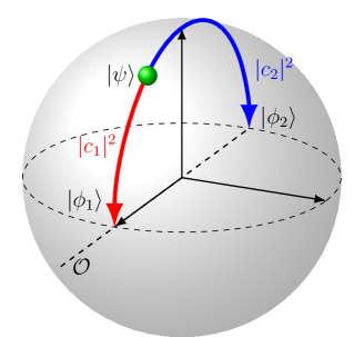
Figure 2: Schematic depiction of the journey to the final states starting from $|\psi\rangle=\sum_{i}c_{i}|\phi_{i}\rangle$ (the green sphere) where $\{\phi_{i}\}$ are the eigenstates of the observable $\mathcal{O}$. $|c_{i}|^{2}$ is the probabilities of the path $|\psi\rangle\rightarrow|\phi_{i}\rangle$. The final state is a mixed state density matrix in accordance with the Born rule.

Degenerate observable and multi-qubit: We extend our analysis to an observable with degenerate eigensystem. We choose a two-qubit system in an entangled state given by,

$$|\psi\rangle=\frac{1}{\sqrt{2}}(|00\rangle+|11\rangle)$$ (19)

We intend to measure $\sigma_{y}\otimes\mathbb{I}$ on this system, such that the measurement takes place only on the first qubit. The eigenvectors of this observable are,

$$|\phi_{1}\rangle = \frac{1}{\sqrt{2}}(|01\rangle-i|11\rangle),\;|\phi_{2}\rangle=\frac{1}{\sqrt{2}}(|00\rangle-i|10\rangle)$$ (20)

$$|\phi_{3}\rangle = \frac{1}{\sqrt{2}}(|01\rangle+i|11\rangle),\;|\phi_{4}\rangle=\frac{1}{\sqrt{2}}(|00\rangle+i|10\rangle)$$ (21)

and the corresponding eigenvalues are, $-1,-1,1,1$, respectively.

The initial density matrix of the system is given by, $\rho_{0}=|\psi\rangle\langle\psi|$. Like the single qubit case, the operation of the observable is emulated by a pulse with flip angle $\kappa$ on the first qubit about $y$-axis . The Hamiltonian corresponding to this pulse is expressed as,

$$H_{\rm\scriptscriptstyle S}=\omega_{1}\frac{\sigma_{y}}{2}\otimes\mathbb{I}$$ (23)

and the time required to apply this pulse is $\kappa/\omega_{1}$.

The system evolves under the Liouvillian obtained using the equation (14) and the final density matrix assumes the form,

$$\rho_{\rm\scriptscriptstyle S}=U\rho_{0}=\frac{1}{4}\begin{pmatrix}(1+e^{-2\omega_{1}\tau_{c}\kappa}C)&-e^{-2\omega_{1}\tau_{c}\kappa}S&e^{-2\omega_{1}\tau_{c}\kappa}S&(1+e^{-2\omega_{1}\tau_{c}\kappa}C)\\ -e^{-2\omega_{1}\tau_{c}\kappa}S&(1-e^{-2\omega_{1}\tau_{c}\kappa}C)&(-1+e^{-2\omega_{1}\tau_{c}\kappa}C)&-e^{-2\omega_{1}\tau_{c}\kappa}S\\ e^{-2\omega_{1}\tau_{c}\kappa}S&(-1+e^{-2\omega_{1}\tau_{c}\kappa}C)&(1-e^{-2\omega_{1}\tau_{c}\kappa}C)&e^{-2\omega_{1}\tau_{c}\kappa}S\\ (1+e^{-2\omega_{1}\tau_{c}\kappa}C)&-e^{-2\omega_{1}\tau_{c}\kappa}S&e^{-2\omega_{1}\tau_{c}\kappa}S&(1+e^{-2\omega_{1}\tau_{c}\kappa}C)\end{pmatrix}.$$ (24)

where, $S=\sin\kappa$, and $C=\cos\kappa$.

In the limit $\omega_{1}\tau_{c}\kappa\rightarrow\infty$, the final density matrix becomes,

$$\rho_{\rm\scriptscriptstyle S}=\frac{1}{4}\begin{pmatrix}1&0&0&1\\ 0&1&-1&0\\ 0&-1&1&0\\ 1&0&0&1\end{pmatrix}.$$ (25)

We can express the above $\rho_{\rm\scriptscriptstyle S}$ as,

$$\rho_{\rm\scriptscriptstyle S}=\sum_{i,j\in\{1,2\}}c_{i}c_{j}^{*}|\phi_{i}\rangle\langle\phi_{j}|+\sum_{i,j\in\{3,4\}}c_{i}c_{j}^{*}|\phi_{i}\rangle\langle\phi_{j}|$$ (26)

where, $c_{1}={\langle\phi_{1}|\psi\rangle}=\frac{i}{2}$, $c_{2}={\langle\phi_{2}|\psi\rangle}=\frac{1}{2}$, $c_{3}={\langle\phi_{3}|\psi\rangle}=-\frac{i}{2}$, $c_{4}={\langle\phi_{4}|\psi\rangle}=\frac{1}{2}$.

The off-diagonal terms will be present in the final form of $\rho_{\rm\scriptscriptstyle S}$ because of the degeneracy between $|\phi_{1}\rangle$, $|\phi_{2}\rangle$ and $|\phi_{3}\rangle$, $|\phi_{4}\rangle$. We can rewrite this as a mixture of the linear superpositions of the states in the following form:

$$\rho_{\rm\scriptscriptstyle S}=(|c_{1}|^{2}+|c_{2}|^{2})|\Phi_{1}\rangle\langle\Phi_{1}|+(|c_{3}|^{2}+|c_{4}|^{2})|\Phi_{2}\rangle\langle\Phi_{2}|$$

where $|\Phi_{1}\rangle=(c_{1}|\phi_{1}\rangle+c_{2}|\phi_{2}\rangle)/\sqrt{|c_{1}|^{2}+|c_{2}|^{2}}$ and $|\Phi_{2}\rangle=(c_{3}|\phi_{3}\rangle+c_{4}|\phi_{4}\rangle)/\sqrt{|c_{3}|^{2}+|c_{4}|^{2}}$ are the normalized superposition states. The application of the drive causes the system to collapse in the degenerate eigensubspaces formed by $|\phi_{1}\rangle$, $|\phi_{2}\rangle$ and $|\phi_{3}\rangle$, $|\phi_{4}\rangle$ with probabilities being $(|c_{1}|^{2}+|c_{2}|^{2})$ and $(|c_{3}|^{2}+|c_{4}|^{2})$, respectively. Therefore, it has been verified that the results of the present example is also consistent with the Born rule.

V Discussions

The principal feature of our model is that the first-order effect of the drive in tandem with the drive-induced dissipation lead the system to a mixed state. It is assumed that the drive is stronger than the system-environment coupling and as such the dissipator from the drive acts before the regular dissipator from the system-environment coupling acts. Also, we require that the drive is applied for sufficiently long duration to reach a quasi-steady-state which is identical to the state predicted by the Born rule. We note that the focus is on the creation of the mixed state through an irreversible dynamics. The lack of an explicit apparatus means that we may not be able to register the outcome of a specific measurement, but that is not what this model intends to achieve. Even if one does not register the outcome of a measurement, a probabilistic mixed state description is reached and one can apply this repeatedly to model the measurement many times without having to reset the apparatus, as shown in the schematics in figure 3. This is one of the major advantages of this model.

One simplifying assumption in this model was $\mathcal{D}_{\rm\scriptscriptstyle S}\gg\mathcal{D}_{\rm\scriptscriptstyle SE}$. In a situation, where the assumption fails, one would expect a competition between the decoherence due to the drive and system-environment interaction. We have shown that similar effect gives rise to the existence of the optimal clock speed for qubit gates in open quantum systems chanda2020 . As a result, the system would end up in a different mixed state which might not be decomposed into the eigenstates of the drive since the system would not be diagonal in the eigen representation of the drive anymore. So, the Born rule might not be obtained in that case. We understand that the Born rule is an asymptotic solution. The system evolves to a steady state no matter whether the drive is strong. If the drive is stronger than system-environment coupling, then only it takes the system to the eigenstates as speculated by the measurement postulate, else the system reaches a different steady state not prompted by the Born rule. We are not actually ignoring the system-environment coupling; rather we confine the FRQME to the drive-drive term only so as to study the nonunitarity induced in the system solely caused by the drive. The DID is scaled by the term $\tau_{c}$ that carries a signature from the environmental fluctuations and determines how fast one can reach a steady state. So, higher $\tau_{c}$ means faster collapse. The emulation of the Born rule is favored at lower temperature.

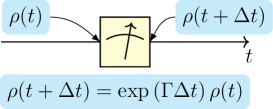
Figure 3: A schematic diagram of the model of the measurement. After the measurement, $\rho(t+\Delta t)$ is of the form predicted by the Born rule. $\Gamma\Delta t$ should be sufficiently large for the system to reach a steady state.

In the year 1991, Milburn proposed a model for intrinsic decoherence based on a simple modification of a unitary Schrödinger evolution and derived an equation of motion for the density matrix of closed quantum systems as a substitution for Schrödinger equation milburn . This is known as Milburn equation. For sufficiently small fundamental time steps with terms up to second order being considered, Milburn equation reduces to FRQME of the form given by equation (5). Few years later, Bu$\check{\rm z}$ek and Konôpka applied Milburn equation to an open quantum system consisting of a two-level atom interacting with single- and multi- mode electromagnetic field buzek . They reported that for very strong system-environment coupling, Rabi oscillation is completely suppressed and the system collapses to a statistical mixture of the ground and excited states. We note that their study focuses on the overdamped nature of the system, but is not a model of measurement process. On the other hand, our model emulates the collapse part of the measurement by presenting a dynamical treatment of how an open quantum system behaves when a drive is applied on it. As per our model, measuring an observable is equivalent to evolving the system under that observable (which happens to be the drive) with a large amplitude, i.e. evolving the system strongly under the observable. This naturally leaves the system in a mixed state formed by the eigenstates of the observable with probabilities given by the Born rule.

VI Conclusion

In this work, we demonstrate that the drive-induced dissipation from a strong drive can result in the emergence of the Born rule in a system weakly coupled to the environment. We assume that the dissipator from the drive is much larger than the dissipator from the system-environment coupling. The resulting dynamics is best analyzed in the eigenbasis of the drive, where, the evolution destroys the coherences. Thus the final density matrix is in a mixed state and is diagonal in this representation for a non-degenerate observable. For an observable with the degenerate eigenvalues, the coherences in the degenerate subspace survives in conformity with the Born rule. This dynamic model emulates the Born rule and could be used repeatedly on a system.

In the quantum information processing, often measurements are included in the quantum circuits. Such measurements could be on multiple qubits and occur more than once in the circuit. Our model could be very useful in simulating the dynamical behavior of a realistic open quantum system which has multiple occurrence of measurements. One would obtain the mixed state representation of the system at the end of the circuit operation, with the added advantage of not having to reset the apparatus. As examples, we have demonstrated the measurement operation for a single- and multi-qubit arrangements.

References

- (1) M. Born, Zeit. Phys. 38, 803-827 (1927).
- (2) C. Cohen-Tannoudji, B. Diu, and F. Laloë, Quantum Mechanics Volume I (WILEY-VCH Verlag GmbH & Co. KGaA, Paris, France, 1977).
- (3) J. Von Neumann, Mathematische Grundlagen der Quantenmechanik, Springer, Berlin, 1932, English translation by R. T. Beyer: Mathematical Foundations of Quantum Mechanics, Princeton University Press, Princeton, 1955
- (4) K. Hepp, Helv. Phys. Acta 45, 237 (1972).
- (5) H. Nakazato and S. Pascazio, Phys. Rev. Lett. 70, 1 (1993).
- (6) M. Cini, Il Nuovo Cim. 73B, 27 (1983).
- (7) H. S. Green, Il Nuovo Cim. 9, 880 (1958).
- (8) B. Gaveau and L. S. Schulman, J. Stat. Phys. 58, 1209 (1990).
- (9) A. E. Allahverdyan, R. Balian, and Th. M. Nieuwenhuizen, Europhys. Lett. 61, 453 (2003).
- (10) W. H. Zurek, Rev. Mod. Phys. 75, 715 (2003).
- (11) W. H. Zurek, Phys. Rev. D 24, 1516 (1981).
- (12) W. H. Zurek, Phys. Rev. D 26, 1862 (1982).
- (13) R. G. DeVoe and R. G. Brewer, Phys. Rev. Lett. 50, 1269 (1983).
- (14) R. Boscaino and V. M. La Bella, Phys. Rev. A 41, 5171 (1990).
- (15) R. Boscaino, F. M. Gelardi, and J. P. Korb, Phys. Rev. B 48, 7077 (1993).
- (16) S. Nellutla, K.-Y. Choi, M. Pati, J. van Tol, I. Chiorescu, and N. S. Dalal, Phys. Rev. Lett. 99, 137601 (2007).
- (17) S. Bertaina, S. Gambarelli, A. Tkachuk, I. N. Kurkin, B. Malkin, A. Stepanov, and B. Barbara, Nat. Nanotechnol. 2, 39 (2007).
- (18) A. Chakrabarti and R. Bhattacharyya, Phys. Rev. A 97, 063837 (2018).
- (19) N. Chanda and R. Bhattacharyya, Phys. Rev. A 101, 042326 (2020).
- (20) A. Chatterjee and R. Bhattacharyya, Phys. Rev. A 102, 043111 (2020).
- (21) H. -P. Breuer and F. Petruccione, The Theory of Open Quantum Systems (Oxford University Press, New York, 2002).
- (22) C. Cohen-Tannoudji, J. Dupont-Roc, and G. Gilbert, Atom-Photon Interactions: Basic Processes and Applications (WILEY-VCH Verlag GmbH & Co. KGaA, Weinheim, Germany, 2004).
- (23) A. Chakrabarti and R. Bhattacharyya, Europhys. Lett. 121, 57002 (2018).
- (24) G. J. Milburn, Phys. Rev. A 44, 5401 (1991).
- (25) V. Buek, M. Konôpka, Phys. Rev. A 58, 1735 (1998).